MSTDP: A More Biologically Plausible Learning

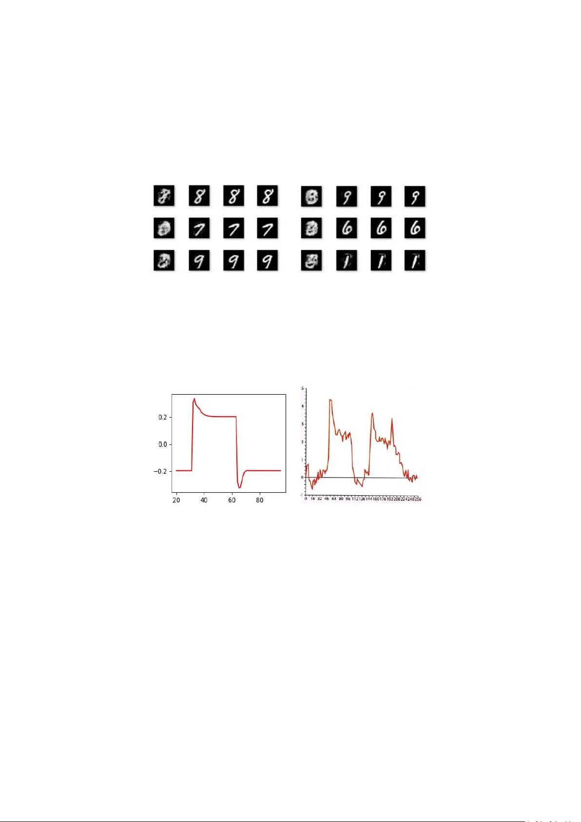
MSTDP: A More Biologically Plausibl e L earning Shiyuan Li Abstr act Spike-timing dependent plasticity ( STDP) whic h observed in the brain has proven to be important in biologic al learning. On the other hand, artificial neural networks u se a different way to learn, such as Back- Propagation or Contrastive Hebbian Learning. In this work, we propose a new framework called m stdp tha t learn al most the sa me way biological learning use, it only uses STDP rules fo r sup ervised and unsuperv ised l earning and don’t need a global loss or other supervise information. The f ramewor k works like an au to-encoder by m aking each in put neuron also an outpu t neuron. It can mak e predictions or generat e patterns in one m odel witho ut additional configuration. We also brought a new itera tive infe rence method using momentum to make the framework m ore efficient, which can b e u sed in training and testing phases. Fina lly , we verified our framework on MNIST dataset for c lassification and generation ta sk. Introd uction Almost every l iving creature h as the ability to learn, but how the brain learns is still u nder studied by neuroscientists. Sp ike-timing depende nt plasticity (STDP) [4, 13, 16] is believed to b e a ke y fundamental of learning process in br ains, and which can be described in very simple mathematical forms [1]. This has major im pact on m odern compu tational neurosci ence becau se it ’ s differ ent f rom common m achine learning algorithms, like Back-Propagation [2], Contras tive Hebbian Learning [5] or Simulated Anne aling [18]. There are so many differences between biolo gical lear ning and learning algorithm s of artificial neural networks. Some properties that biologica l learning has but mac hine learning don’t are: (i) the in format ion needed for one neuron to perform learning a lgorithms is all in that neuron. It doesn’ t require other information like a glob al loss or p ost synapse neuron behavior . Neurons also don’t nee d the information to tell them when to learn, like clam ped phase or free phase in Contrastive Hebbia n Learning (ii) There is no difference between the training process and the in fer ence process. Animals d on't distin guish training or testing, they are learnin g every moment and u sing what they have learned ever y m oment. The training process just fed data into the model, a nd the model will lear n on its own. (iii) Some observed biological characteristics, like asymmetric weights and temporal dynamics of neurons (when a neuron is activated, it first violently spikes and then drops to a value higher than th e inactive state. Also, when a neuron is inactivated, it first strongly suppressed a nd then increases to a value below th e ac tivation state). There are many mac hine Learning algorithms that can satisf y some of the p roperties above. The targe t propagat ion algorithm [12] com putes local er rors at each lay er of th e network using information about th e target, which not nee d a glo bal loss but still need the loca l post synapse neurons to propagat ed er ror signal. The recirculation algorithm [11] don’ t need any other information bu t the derivatives of the neurons, u nfortunate ly it need symmetries weight. The Contrastive Heb bian lear ning (CHL) [ 5, 14, 15] whi ch based on the Hebbian learning rule does n ot require k nowledge of any derivatives. However , CH L have to tell the network to do diffe rent algorithms in clam ped phase an d free ph ase and it also requires synaptic symmetries an d it need post synapse i nformation. Others [17] use difference as a target to perform back -propagation. It has asymmetries weight, b ut the learning method is d iffe rent from real neurons. All algorithms above have d iffe rent training and infe rence pr ocesses, and they d on’t have the temp oral dynamics. In this paper , we proposed a new learning f ramework called Momen tum Spike-timing dependent plastic ity (mstdp), it satisfy all those properties above and h as the same performan ce as existing mach ine learni ng algorithm s. The mstdp method requires only the in put of the neuron and derivative of the neuron to perform learning. There is no diffe rence between the training process an d in fer ence process, and it doesn ’t need symmetric weights and has n eural temporal dynamics. Artificial neural networks comm only use diffe rent learning algorithms for supervised or unsuperv ised learnin g. While brain can also p redict or generate, but do esn’t distinguish between supervise d or u nsupervise d learning. Animals learn their environment to surv ive and evolve, but they doesn' t hav e a teacher or superv ise informa tion. Human babies m ay lear n how to talk f rom their parents, but parents can’t teac h them how to see and hear . When a parent teaches a baby by pointing at a d og, they di dn’t te ach the neurons in b aby ’ s brain th e mean ing of dog, they just linked th e look of a dog an d the sound of the word “ dog ” in the b aby ’ s brain. So we think there is no real sup ervise learning in biolog ical learn ing, they just lear n to lin k information and adapt to the envir onment, just like unsupervised lear ning algorithms learn to adapt to the data. Motivated to c reate a more biologically plausible learning , we conv ert su pervised learning problem into a unsuper vised learning problem by making in put neurons in the network a lso output neurons. Which is same to b iological observations that photoreceptor n eurons also ha s feedback connections. The m odel performs unsupervised learning like an auto-encoder by concatenate the in put data with the labels. This automatically make prediction problem a in-painting problem by clamped the input data to get th e labels. We can also generate samples from the model by clamped the label to get the input data. The ab ove modific ation will make it difficult for the model to converge. We solve this by add momentum in the iterative infer ence. Momentu m Stochastic Gradient Descent is a well-known method for training Back-Propa gation neural networks, It can effectively sol ve the problem of training jump into a local minim um. It can also be used for iterative inference processes to get better result. We use m omentum itera tive inference for both training and infere nce. We a lso smoothing the path in d iffe rent state of the network to speed up the infer ence process. The proposed learning framework can solve diffe rent problems, we verified it on MNIST dataset for c lassification a nd generation problems. Model and M ethods 2.1 Model We use the sa me m odel as [6], Suppose there are several n eurons in th e network, Ever y neuron has an internal state s , every two neurons a re co nnected with a weight, and every neurons has a bias. Classical leaky integra tor neural equation is u sed to calculate neurons behaviors. It follows: ) ) ( ( i i i s s R dt ds    (1) where R i (s) represents the pressure on neuron i from the rest of the network, while ε is the time const ant parameter . Moreove r , suppose R i (s) is of this form: ) ) ( )( ( ' ) ( ,     i j i j i j i i b s W s s R   (2) Where W j,i is the weight from the j th neuron to the i th neuron, b i is the bias of the i th neuron and ρ is a nonlinear fun ction. The pu rpose of th is formula is to go down the energy func tion, which is d efined by [ 6]:        i i i j j i i j i i i s b s s W s s E ) ( ) ( ) ( 2 1 2 1 ) , ( , 2     (3) Where θ is the parameters in the m odel, in this c ase W and b . Derive E with respect to s a nd with (1), we can get: ) , ( s s E dt ds       (4) So the dynam ics o f the network is to per form Gradient Descent in E , each fixed-point for s will correspond to a local minimum in E . 2.2 STDP rule Spike-Timing Dependen t Pla sticity (STDP) is considered the m ain form of learnin g in brain, it relates the cha nge in synaptic weights with the timin g difference between sp ikes in post synaptic neurons and pre synaptic neurons. Experime ntal in [1] show tha t the stdp rule can also be form as: dt ds s dt dW j i j i ) ( ,   (5) Where α is the learning ra te. In this paper , we ch ange the form of stdp rule to: t s s t W j i j i      ) ( ) ( ,   (6) Which is m ore sim ilar to the CHL rule since: ) ( ) ( )) ( ) ( ))( ( ) ( ( ) ( ) ( ) ( ) ( j f i f j j f i i f j f i f j c i c s s s s s s s s s s                  ) ( ) ( ) ( ) ( ) ( ) ( j i j j f i i f s s s s s s              Where ρ c is the clamped phase f ixed-point an d ρ f is the free phase fixed-point, we ignore the term Δρ (s i )Δρ(s j ) and get (6). Differ ent from CHL, we don’t learn on ph ases. Every iteration will perform this learn rule , and the clamped phase and free pha se are auto turn after a fe w iterations, don’t sy nchronou s to data. Every da ta have several clamp ed phases and free pha ses. Therefor e, the overall learning rule for i th neuron in th is paper are: ) ( ) ( , j i j i s s W       (7) ) ( i i S b      2.3 Ad d in puts There are some input neurons in the network, so we split s into two parts, s vis and s hid , s = (s vis , s hid ) . For the input neurons s vis we ad ded another pressure to push it towar ds the input d ata: ) ( i i i s data dt ds    (8) Where data i is the input d ata for the i th input neuron. Which is equivalent to add another term i n the energy function E :            vis s i i i i i i j j i i j i i i s data s b s s W S s E 2 , 2 ) ( 2 1 ) ( ) ( ) ( 2 1 2 1 ) , (      (9) This is the same idea as in [7], the differen t between us is th at β in this paper is not inf inite for input neurons, and we d on’t distin guish input and output. We define:     in s i i i s data s dat a C 2 ) ( 2 1 ) , (  (10) So the training process is to make C smaller . 2.4 Momentum infer ence We use m omentum to help iterative inference, so we change (1) into: i i v dt ds   (11) Where v i is the velocity for s i , an d we update v i use: 1 ) 1 ( ) ) ( (      t t i i i i v m s s R m v (12) Where m is the inertia parameter . 2.5 T rai ning For training, we first initialize W an d b randomly , and also randoml y ch oose an s as initial. Than we choose a data sample, set β to a positive value and do a fe w itera tion, like the clamped pha se in CHL. During the clamp ed phase we change W , b use (7) at every iteration. After that we set β to a 0 and do a few iteration, l ike the free pha se in CHL. W e repeat those c lamped phase and free pha se several times with the sam e data. We loop this process for each data until c onve rgence. The wh ole algorithms is demonstrate in algorithms 1. Algorithms 1: Momentum Spik e-timing Dependent Plasticity , ε is the iter ation st ep for s to decrease E , β is the iteration step for s to decrease C , α is learning rate, epochs is training tim es, T is the times we do clamped ph ase and free phase for each data, iteration is iteration tim es in each relax ation. Require: ε , β , α , epochs, T , iteration Initialize W , b an d s randomly for n ← 1, . . . , epochs do data = data n for t ← 1, . . . , T do β = 1.0 for i ← 1, . . . , iteration do Update s use (11) Update W , b use (7) end for β = 0.0 for i ← 1, . . . , iteration do Update s use (1) end for end for end for Notice that we don’t reinitialize s af ter data chan ged, so the first clam ped p hase and free phase will change s from one f ixe d-po int to a diffe rent fixe d-po int. This m oving path will also be learned by the stdp rule. The frequenc y neurons change c lamped p hase in to free phase doesn’t related to the frequency we cha nge data, just like in biologically learning process we can’t teach the neurons when to lear n in c lamped phase or free pha se. 2.6 T est ing The test process is same to training process, except the lear ning rate is zeros an d we ca n do fewe r clamped and free phases. 2.7 Smooth ing deri va tive We also smoo thing th e path between d iffe rent fixed-points by make d erivative o f every point on the p ath smaller , in order to make the network easier to ju mp from one fixed-point to another fixe d-poin t. We perform this by calculate the derivative of ds to W , a djust W to ma ke ds smaller . ds is: s b s W s ds i j i j i j i i      ) ) ( )( ( ' ,   (13) So the derivative of ds to W , b is: ) ( ) ( ' , 2 j i j i s s W s E       (14) ) ( ' 2 i i s b s E      (15) And the learning rule will be: ) ( ) ( ' , j i j i s s W     (16) ) ( ' i i s b    (17) This will make the path between differen t fixed-points flatter and easier to jump. 2.8 Why t his work In the beginning , the model had so me fixed-point and they didn’t make any sense. By clamped the input neurons to d ata, we end up with a f ixe d-po int tha t ha s low C to the cu rrent data. In each iteration, the learning rul e will m ake the output of the neurons m ore like the next itera tion’ s ou tput, so the whole learning process will m ake the network easier to jump from the old fixed-point in to the new fix ed-point. When the jump is from a free fixed-point into the clamped fixed-point, it will m ake the free fixed-point has lower C. When the jump is from one data’ s fixed-point into another (for example, from data i ’ s fi xe d-point to data j ’ s fi xe d-point), the opposite jump will cancellation the learnin g (from th e data j ’ s fixed-point into data i ’ s fixed-point). So, from all, we make every data’ s f ree fixed-point has lower C . Therefor e, with those free f ixed-points, the network can get some meaningful outpu t without input. Just like humans can im agine things with their eyes clo sed, which is a property not find in other methods [5, 11, 12, 14, 15]. It h as been proved that random feedback can play the same role as back -propagation [8,9]. So af ter training these input neurons will have the same value for the input data, and C will become very sm all. The training process will create m any fixed-points. When da ta cha nged, the new pressure of C drives s to leave the old fixed-point, and the pressure of other neurons will stop it from leave the current f ixe d-po int. The for ce of C is usually not big enough to make s to jum p out of current fixed-point, that ’ s why we need the mom entum to help it jump. The training process will pick the fixed-points that is easy to ju mp and make it h ave a lower C. Result In this section, we will verify our algorithm on classification tasks and generation tasks. The dataset we use is the MNIST Handwr itten Digit and Letter Classif ication dataset. The neural network has 784 + 10 input neurons for da ta and labels and the number of hidd en neurons is 2048. Each input neuron is c onnected to all h idden neurons, a nd all hidden n eurons are interc onnected, but input neurons don’t connected to each other . We train our model on 10000 numb ers for 500000 times and test on 500 numbers. We d on’t train with batches, which makes training a nd tes ting the sa me. The lear ning ra te we use is 0.001 and there are 10 clamped and free phases for each da ta. For champed phase s, ε is 0.2 , β is 0.8 and m is 0.4. For free phases, ε is 0.2, β is 0 a nd m is 0. We use sigmoid4 as activate functio n to speed up the training process, which is sligh tly differ ent form the sigmoid function (sigmoi d4(x) = sigmoid(4x)). Parameter s W and b are initialized with a uniform distributions U ( − 0.1, 0.1). For each clamped and free p hase, we iterate 32 times to get s . 3.1 Classi fication We clamped the inpu t d ata and labels in training and only cla mped inp ut d ata an d do three clamped pha se and free phase to get the labels in testing. After training, it has an accuracy of 100% on the training set and 96% on the testing set. Figure 1 shows the free phase fixe d-point, 1 st clamped phase fi xe d-poi nt, 2 nd clamped phase fixed-point and labels in a training loop. The free phase f ixe d-p oint is m eaningless, but after jumping it will end up in a fixed-point pretty close to the label. Figure 1 there are 6 groups of data in the figure, for each group of data, from left to right: (a) random fixed-poi nt. (b) 1 st fixed-poi nt after the clamped data. (c) 2 nd fixed-poi nt after clamped data. (d) labels The biological neurons have temporal dynamics, and m omentum infere nce c an lead to the same result. Figure 2 shows the similarit y between mom entum infere nce and real neurons. Lef t is the simu lation in our p aper , right [10] is th e response of a real biological neuron to certain featur es. X axis represents time an d Y axis represents intensity . Figure 2 left: simulations by the model. right: response of a real neurons. 3.2 Generation We can generate samples by randomly pick a fixed-point, b ut this usually get mean ingless samples (figure 1 a ). So we use condition al generation method to generate numb ers by f irst randomly pick s and then d o a few clam ped and free p hases with label clamp ed. The label will constrain the distribution of hidden neurons to get m ore reasonable result, so the network will jump to a number loo ks image in that label. Figure 3 shows som e samp les generated by our model. Figure 3 some numbers generat ed by our model Discussion In this work, we introduced a framework for supervise d learning and unsu pervised learning. The wa y it learns is very similar to biologic al learning. But there are still some dif ferences between the framework and real neurons: (i) real neurons has sparse representations, but our framework doesn’ t. (ii) in our framework, the network will finally stay at a f ixed-point and no longer jump. But brain never stop thinking even witho ut inputs . Instead, focus on on e thing is difficult. For (i), real neurons consume energy whe n they spike, and energy is precious to wild animals. Sparse represent ation make fewer neurons spike, which will help th em save energy . So, whether sparse representat ion is h elp for better representa tion or ju st help for save ene rgy still needs discussion. For (ii), sta y at one fixed-point doesn’t help animals for r apid response to dangers in environment, so there mu st be som e mechan ism to h elp it jump out a f ixed-point if stay s in it too long. Real neurons will becom e tired when they spike. This m ay lead to a reduction in spikes an d make it hard to sta y in a fixed-point. On the oth er hand, the math in (4) has some approximations, the derivative of E is actually: ) ) ( ) ( 2 1 )( ( ' , ,      i j i j j i i j i i b s W W s ds dE   We use W ij instead of (W ij +W ji )/2 to simplif y the calculation. If we consider s as a force, the space of s will become a force f ield. When the curl of the f ield is no t ze ro, particles in th e force field may move for ever . The c url of the f ield is alway s zero whe n we use (W ij +W ji )/2 , but not always zero when use W ij . This may also cause the network not stay . The framework works like an a uto-encoder network, which usu ally have a bottleneck. If an auto-encoder doesn’t have a bottleneck, the network will tend to be trained i nto an identity map for every dat a. But bottlenecks also reduce the representation ability of the n etwork. Ou r model may be a solution of this since the number of hidden neurons of our mod el can be greater than the number of dim ensions of the input data. Generating num ber images by randomly pick a fixed-point will get meaningless sam ples. This is due to the super fluous fixe d-point that don’t match any data. However this will make bad influence to the performance of the network. How to avoid this will further study in the future. Ref erences [1] Y Be ngio, T Me snard, A Fische r , S Zhang, Y Wu, STDP as p resynaptic activity times rate of change of po stsynaptic ac tivity . arXiv preprint arXiv:1509 .05936. [2] Y LeCun, BE Boser , JS Denker , Han dwritten digit recognition with a back -propagation n etwork, Advances in Neural Information Processing Systems, 1990 [3] JR Movellan, Contrastive Heb bian Learnin g in the Continuou s Hopfield Model, Connection ist models, 1991 [4] G Bi , M Poo , Synaptic modi fications in c ultured h ippocampal n eurons: depende nce on spike timing, synaptic strength, and postsynaptic neurons type. Journal of neuroscience, 18(24):1046 4-10472, 1998. [5] P Baldi, F Pineda , Contrastive le ar ning and neural oscillations. Neural Computation, 3(4):526– 545, 1991. [6] Y Bengio, A Fischer , Early inference in ene rgy-based m odels a pproximat es back -propagation. arXiv preprint a rXiv:1510.027 77. [7] B Scellier , Y Bengio, T o wards a Biologically Plausible Back prop, a rXiv:1602.051 79, 2016 [8] TP Lillicrap, D Cownden, DB Twe ed, Random fee dback weights sup port learning in deep neural networks, arXiv preprint arXiv :1411.02 47 [9] G D etorakis, T Bartley , E Neftci, Contr astive Hebbian Learning with Random Feedback Weigh ts, Neural Networks, 2019 [10] M Gazzaniga, R Ivry , G Mangu n, Cognitive Neuroscience The Biology of the Mind, page 162. [11] G Hinton, J McC lelland, Learning r epresentations by recirculation. In Neural info rmation processing sys tems, p ages 358–366, 1988. [12] D L ee, S Zhang, A Fischer , Y Bengi o. Differ ence target propagation. In Joint european confe rence on machine lear ning and knowledge discovery in da tabases, pages 498–515 . Springer , 2015. [13] H Mar kram, J L¨ubke, M Frotscher , B Sakman n. Regulation of synaptic efficacy by coincidenc e of po stsynaptic ap s and epsps. Science, 275(52 97):213– 215, 1997. [14] JR Movellan. Contras tive hebbian learning in the continuous hopfield model. In Connectionist models: Proceedings of the 1990 summer school, pages 10 – 17, 1991. [15] X Xie , H Seung. Equivalence of bac kpropagation and contrastive h ebbian learnin g in a layered network. Neural computation, 15(2):441 – 454, 2003. [16]L Zhang, W T ao, C Holt, W Harris, M Poo. A c ritical window for coopera tion and competition among developing retinotectal synapses. Nature, 395 (6697):37, 1998. [17] Y Be ngio, DH L ee, J Born schein, T Mesnard, T owards b iologically p lausible d eep learnin g, arXiv preprint a rXiv:1502.041 56 [18] E Aarts, J Korst, Simulated annealing and Boltzmann ma chines, 1988