Online monitoring of local taxi travel momentum and congestion effects using projections of taxi GPS-based vector fields

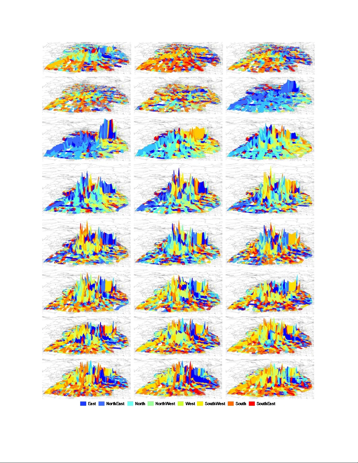
1 Online monitoring of local taxi travel momentum and congestion effects using projections of taxi GPS-based vector fields Xintao Liu PhD, Assistant Professor Department of Land Surveying and Geo-Informatics, The Hong Kong Polytechnic University, Kowloon, Hong Kong xintao.liu@polyu.edu.hk Joseph Y.J. Chow PhD, Assistant Professor & Deputy Director C2SMART University Transportation Center Department of Civil & Urban Engineering, New York University, New York, NY, USA. Corresponding author: joseph.chow@nyu.edu Songnian Li PhD, Professor Department of Civil Engineering, Ryerson University, Toronto, ON, Canada snli@ryerson.ca Acknowledgements The authors wish to th ank the DATATANG Comp any for the real -time GPS data used in thi s stud y. Dr. Xintao Liu acknowledges the funding support from an A rea o f Excellence project (1- ZE24) and a startup project (1-ZE6P). Dr. Chow is partially supported by th e C 2 SMART Tier 1 Universit y Transportation Center, which is gratefully acknowledged. The Conflict of Interest The authors declare that there is no conflict of interest regarding the publication of this paper. Accepted for publication in Journal of Geographical Systems 2 ABSTRACT Ubiquitous taxi trajectory data has made it possible to apply it to different types of travel analysis. Of interest is the need to allow someone to monitor travel momentum and associated con gestion in any location in space in real time. However, despite a n abundant literature in taxi data visualization and its applica bility to travel analysis, no ea sy method exists. To measure taxi travel momentum at a location, current methods requir e filtering taxi trajectories that stop at a location at a particular time range, whic h is computationally e xpensive. We propose an alternative, computationally cheaper way based on pre -processing vector fields from the trajectories. Algorithms are formalized for generating vector kernel densit y to estimate a travel-model-free vector field-b ased r epresentation of travel mom entum in an urban space. Th e algorithms are shared online as an open source GIS 3D extension called VectorKD. Using 17 million daily taxi GPS points within Be ijing over a four-day period, we demonstrate how to generate in real time a series of projections from a con tinuously updated vector field of taxi travel momentum to quer y a point of interest anywhere in a cit y, such as the CBD or the airport. This method allows a polic y-maker to automatically id entify temporal net influx es o f travel demand to a location. The proposed methodology is shown to be over twent y times faster than a conventional selection quer y of trajectories. W e also demonstrate, usin g taxi data e ntering the Beijing Capital I nternationa l Airport and the CBD, how we can quantify in nearl y real time the occurrence and magnitude of inbound or outbound queueing an d congestion periods du e to taxis cruising or waiting for passengers, all without having to fit any mathematical queueing model to the data. Keywords: GIS, vector kernel density , spatial anal ysis, trave l pattern, Beijing, taxi data 1. Background Increasing urbanization and population growth contribute to increasingly negative externalities in cities: congestion, pollution, and vulnerability of the popu lation and economy to extreme events. The rise of Big Data ( Tansley a nd Tolle, 2009) , especiall y human mobility data at the city-scale, presents a potential solution to co pe with the se problems. Having access to real- time locations of people throughout the city circumvents the need to connec t traffic patterns to travel (and economic ) patterns, a nd instead dire ctly connects a rea l- time data source to the “pulse” of the ec onom y . This causes a paradig m shift that prese nts a n opportunity in how w e visualize and quantify travel demand patterns through space-time. One such popular data source is from taxi GPS trajectories (see Yue et al., 2014, for a comprehensive surve y) . For planning purposes, taxi GPS da ta ca n be used to mine origin- destination patterns, time of day variations for specific locations, hotspots, tr ip dist ances, etc. (Yu e et al., 2009; Z heng et al., 2011; Huang et al., 2015; Tang et al., 2015; Mao et al., 2016; Shen et al., 2017); to cluster land use types ( Liu et al., 2015); and to identif y critical locations or quantify resilience (Zhou et al., 2015; Zhu et al., 2017). These objectives have b een addressed with other similar data sources, such as call detail records (CDRs) (Toole et al., 2015). In all the above studies cited, the use of the taxi trajectory data is for planning purposes only. They are not designed fo r online operations such as city monitoring (Chow, 2 016), e.g. quantif y ing 3 the effects of major incidents or weather in real time as they occur and que rying spatial-temporal congestion patterns to identify bottlenecks to condu ct remedial operational strategies . Fo r example, if a us er wanted to que ry all the arrivals and departures from a particular point of interest (POI) during a specific time interval, it would have to run a s earch through every taxi trajector y to filter out the ones that pass through that sp ace-time perimeter. This is extremely computationall y expensive, and thus can only work for planning purposes. Non etheless, city monitorin g is necessary for a smart city to thrive and t axi data can help fulfill that role (Sayarshad and Chow, 2015). No example is more evident of this need than the whole theor y of mac roscopic/network fundamental diagrams. This theor y has aris en significantl y in the last few years because of the importance of monitoring congestion at a city wit hout having to pay specific atten tion to specific road facilities (e.g. Geroliminis and Daganzo, 2008 ; Da ganzo and Geroliminis, 2008; Mahmassani and Saberi, 2013) due to the availability of large scale urban data. However, netwo rk fundamental diagra ms de pend on monitoring vehicles entering and exit ing a pre-defined bound ary and does not consider spatial proximity. Another e xample of such an ef fort to measure dynamic activity changes using taxi trajectories is that of Scholz and Lu (2014), although their work is limited to only hotspot chan ges and in terms of offline analysis. An online methodology is needed to allow a user to monitor traffic congestion considering spatia l proximit y and query metrics for any local POI of interest. One relevant a rea of r esearch is the vectorization of taxi trajectories. Liu et al. (2012) proposed doing so for taxi trips within a time geographic ( Hägerstrand, 1970) context so that a dist ance decay distribution law could be derived. They found that a Lév y flight distributi on c an be used to model these trips using da ta from Shanghai, C hina. Vectorization is potentiall y an effective method because dir ectionality of trip demand can be stored at a unit interval, and then very fast computations can be run using vector c alculus (integrals, summations, dot products to p roject vectors onto other directions, etc.). The use of vector fields in urban setting began in the early 1970s, through the work of Angel and Hyman (1970, 1976) to construct “velocity fields” . Puu and Beckmann (1999) envisioned time -space a s a c ontinuous space. Miller and B ridwell (2009) proposed a more generalized vector field theory to characterize time-geographic urban space, which is a kind of vector GIS method that considers both scalar densit y and dir ectional cost functions — a field theor y for individuals. Liu et al. (2014) ex tend ed the field theory to a population, as a “momentum” of travel demand, leading to a momentum vector field. In physics, momentum is the product of ma ss and velocity. For travel demand mom entum, the “mass” is the population while the “velocity” is the trave l velocity within a space-time domain. The autho rs estimated this vector field using 3D kernel density, called vector ke rnel densities. A primar y advantage of such an approach is that all the inherent directionalit y in the demand, typically stored in high dimensional OD matrices, is now preprocessed into unit vectors in a time-space field. The result is that a query (for operational purposes) for travel momentum toward a pa rticular POI in time, for example, can simply b e computed by running a projection of the ve ctor fi eld toward that location in time -space. Th ere is no need to query individual trajectorie s to see if they fall within so me thresholds, mar king this study as the first to allo w GPS trajectory data for spatial-temporal moni toring for op erational purposes. As an analogy, the construction of a vector field (and its subsequent online updating) is similar to storing in memory the demand patterns of the system of interest so that spatial-temporal queries can be readily extracted. While L iu et al. (2014) demonstrated the methodology using a proof of concept from Toronto travel survey data , it was never applied to taxi G PS data in an onli ne framework. I n the case of 4 taxi s y stems, an addition al unique qualit y is that t he inbound and outbound flows for an y given POI is ty pically cons erved over a long enough period of time, since taxis do n’t gen erally park long term. As a result, being able to quer y taxi momentum projections onli ne has at least two useful purposes: (1) it allows a user to monitor hotspots dy namically so that operational strateg ies can be implemented, and (2) in doing so it can qu antify in re al ti me the taxi queueing bottlenecks that may occur at an y POI upon request. No other study, to the best of the authors’ knowledge, has done this before. We propose guidelines f or how to use thi s method for any real-time GPS data set around th e world. We formalize a set of algorithms for generating vector kernel density based on the methodology f rom Liu et al. (2014) and then develop an int egrated 3D anal ysis GIS package called VectorKD . VectorKD is an open source project that is available for further ex tension and validation for general purposes in related urban studi es. Ve ctorKD is a pplied to a data set of twelve thous and Beijing taxis conducting over 17 million daily trips. This allows us to demonstrate how we can identify in real time when taxi congestion effects at a local POI may begin to occur. The remainder of this pa per is organized as follows. Section 2 provides a simple description of the study area and data sourc es, presents the formalized alg orithms for ge nerating vector ke rnel density, followed b y the vector kernel densit y projection as a part of the ex perimental methodology. Section 3 illustrates the results of the experiments using real-time GPS trajectories of taxis in Beijing, China. Section 4 concludes the paper. 2. Methodolog y The theor y b ehind the methodology of the vector fields is discussed in L iu et al. (2014), which proposes a popul ation-based vector field fo r visualiz ing and representing ti me-geographic demand momentum. The field is estimated using a vector kernel densit y generated from observed trajectories of a s ample population. For more details, please refer to the original work b y Liu et al. (2015). The key term to note is that of “t ravel momentum”, which is a vector determined b y th e product of a scalar population demand and a vector travel spe ed. Tra vel momentum is re presented as a vector field, which in practice involves separating disc rete cells, or “taxels” , for each unit of time -space, and using vector kernel densities to es timate the vector field within each taxel from the taxi GPS sample data. 2.1. Generating the vector kernel density Based on the real-time GPS da ta, we generate ve ctor kernel density as a continuous re presentation of taxi trave l momentum. Pseudo codes are provided to better illustrate this method. The generation of the vector kernel density is divided into four steps in our work. First, we decompose the continuous 3D ti me geographic urban space int o quantitative units: 3D cubes or “taxels” . W e use a grid to r asterize the 2D geographic space i nto cells (see Fig. 1a), given a spatial resolution (e.g., 100 meters). Then we use a sizable time unit/resolution (e.g., one minute or one hour) to de compose the continuous t ime dimension into discr ete time slots, (e.g.,   to   in Fig. 1a). 5 Fig. 1 . (a) Sp litting trip vectors with time slot; (b ) How line based kernel densit y works ; (c ) Vector addition for vector based kernel densit y. Second, we clip the travel vectors within eac h time slot. A travel vector (red soli d lines in Fig. 1a) refers to two consecutive GPS points in a taxi trajector y . Such a travel vector has a start time as well as an end time, based on which we can select all travel vectors overl apping with a time slot in time dimension. If the time slot does not completel y cont ain a trip vector (e.g., Trip Vector A in F ig. 1a), we clip the trip vector b y time ratio. All the trip ve ctors within the current time slot are projected (blue solid lines in Fig. 1a ) onto the 2D space. x y time t 1 t 0 Time slot Travel Vector A Travel Vector B (a) (b) (c) 6 Third, we generate a 2D kernel densit y map for each time slot . In Fig. 1b, it shows how the kernel densit y m ethod works for 2D lines in 2D space. Con ceptually, a smooth curved surface is created over each li ne within a given search radius (e.g., 100 or 1000 meters in Euclidean distance). The surf ace has the highest densit y value at the location of line and the v alue dim inishes with increasing distance from the line and rea ches zero at the radius dist ance. The closer the cells to the line, the higher the density value they have. If there are more than one line, we can simple add up all density value for each cell. In doing so, we can get a 2D kernel densit y estimation. Fourth, we vectorize the 2D kernel density map. To add a vector dimension to the 2D kernel density map, we use travel vectors to generate a new vector for each cell. In Fig. 1c , it shows the conceptual process to calculate such a n ew v ector for a cell. Suppose there are two travel vectors (blue solid lines A and B in Fig. 1c) that are within the search radius from the cent er point of the cell (bold square with a black dot cent er in Fig. 1c). For e ach of these two travel vectors, we can make a p arallel v ector th at starts from the cent er of the cell: the short dash ed blue arrow is the parallel vector of Trip Vector A and the long one is the parallel vector to Trip Vector B. Using vector addition, we c an ge t a new added-up vector (dot red arrow). In doing so, we obtain the directional vector for the cell (i.e., the direction of the new vector). By combining the 2D d ensity value and the cumulative vector toge ther, we get the vector density estimation for each taxel. The following pseudo code in Algorithm 1 is p rovided to summarize the above four-step method. We use R a s the bandwidth (or search radius) for a number of lines within a time slot a nd use cell_size to rasterize the 2D space into cells (or grid). The minimum and max imum coordinates are ( m in_x , min_y ) and ( m ax_x , m ax_y ) of the 2D spac e and the number of travel vectors is N . The vector formula for the i th trip vector is: ( x i0 , y i0 ) for start point and ( x i1 , y i1 ) for end point. Algorithm 1: Generate vector kernel density For (x = min_x; x < max_x; x+= ce ll_size ) { For (y = min_y; y < max_y; y+= ce ll_size) { Cx = x + cell_siz / 2.0; // center x of current cell Cy = y + cell_siz / 2.0; // center y of curr ent cell For (i = 1; i<= N ; i++) { r = distance from c urrent c ell center ( Cx, Cy ) to cur rent trip line; If (r <= R) { KDE = 21.75 / ( π * R 2 ) * ( max (0, 1 - r 2 / R 2 )) 2 ; // Quartic kernel den sity C (i, j) += KDE ; //Add the KD value to cel l kernel densi ty C (i, j) NV = [( x i1 - x i0 )/ r , ( y i1 – y i0 )/ r ]; // normalized paralle l vector of cur rent trip line CV (i, j ) = [ Cx+ ( x i1 - x i0 )/ r , Cy + ( y i1 – y i0 )/ r ]; //Add NV to cell ve ctor CV (i, j) } } } } There w ill b e m cell s a long x and n cells al ong y, and number of travel vec tors N, which is m *n*N in total. And these processes will repeat for each tim e slice. I t should be noted that: (1) the quadratic Kernel Densit y Estimation ( KDE ) function in the pseudo code can b e changed to an y other 7 function such as Gaussian or uniform ones; and (2) the generated results can be saved either in self-defined da ta formats (e .g., XML), in an existing GIS data format (e.g., ESRI g eodatabase), or a combination of the two. The vector kern el density in a taxel is an estimate of the tax i travel momentum vector of the underlying transport system at that location in ti me-space. It includes a net direction from the population as well as a net magnitude. The higher the population demand for travel in that direction at that point in time-sp ace, the l arger the vector. T he hi gher the speed of tra vel, the lower the slope along the time-axis, and therefore also the larger the size of the vector. 2.2. Projection of vector kernel density The gene rated vector kernel densit y represents the taxi travel momentum in the study area. As a vector field, the deman d directionalities are now stored in a much mor e compact data structure that does not require embedding an y travel demand model to quantify spatial-temporal patterns . Every point in space over time of day has a vector density (if done in real time, they would update along the time of day axis), which means both the mag nitude of the de nsit y and dire ction of travel demand are available to use. One new application that we propose in this study is the projection of the vector onto any POI by request in real time. The process is shown in Fig. 2. Suppose we have a POI (red point at the center) and we need to p roject vector kernel dens ity of four cells onto it . For cell A, we connect the center of cell A to the PO I to form a Cell-POI vector (green solid arrow li ne), based on which the vector kernel density of cell A (red solid arrow line started from center of Cell A) can b e projected onto the cell-POI vector as the dashed blue arrow line (also started from Cell A). Mathematically, the abov e process is the dot product of Cell-POI vector      󰇟 󰇠 and cell vector      󰇟 󰇠 . By repeating the above projection process, we can g et all projected ve ctors of the other cells to the PO I and then add up all projected vectors to get an accumulated vector kernel density VKD by using Eq. (1 ).   󰇛           󰇜    (1) where  is the number of c ells within search radius f rom the current cell, 󰇟󰇠 is th e   Cell- POI vector, and 󰇟󰇠 is the cell vector as mentioned ab ove. Note that the search radius ma y be set to be a threshold defined b y an appropriate distance deca y rate if known (e.g. Liu et al., 2012). Computationally, note that this is much faster than the conventional proc ess of checking each existing GPS trajectory to see if and how the y align with a PO I, as th e computation onl y requires vector operations. The direction of the projected v ector of a Cell to a POI c an be either oppo site to or towards Cell-POI vector. If th e direction is opposite, it means the potenti al travel momentum will be decreased from this POI , e.g., Cell A and B. On the contrary , the projection of ce ll vector can also be towards the PO I, whi ch means the potential increased trav el demand to the P OI, e.g., Cell C and D. B y calculating the projection vector that are awa y from and tow ards a PO I separately, we can distinguish “inbound ” and “outbound” travel momentum to evaluate the patterns of POI. B y plotting the two values together over time, it is possible to monitor inbound and outbound travel momentum, and to identify differences. The area under between inbound and outbound projected momentum along the time axis is the numerical integ ral that can be calculated using Eq. (2). 8 Fig. 2 . Pr ojection of vector kernel density onto Point of In terest (P OI) as travel momentum.          (2) where  is number of time slot s minus one,   is the in ternal width b etween two consecutive time slots, and   is the average density difference o f such time slots. Suppose the inbound and outbound travel momentum areas are calculated as   and   . The changing rate o f tr avel momentum between two sets of time slots can be evaluated using the following Eq. (3 ):            (3) Note that if the outboun d area be comes ver y small, the Rate will spike up t o infinity, and when it is exactly zero the Rate would be undefined. This provides a user with a tool to automaticall y identify congestion events with re spect to POIs and deplo y different remedial strategies depending on whether the inefficiencies are ca used b y inbound or outbound c ongestion. More formally: Definition 1 : A projection of a ve ctor kernel densit y of the tax i travel demand momentum to or from a POI measu res the combined demand a nd efficiency to us e the underly ing transport system to get to or from the POI. A larger proj ected value indicates either high demand, high efficienc y in travel speed, or both. 9 Definition 2 : A projection profile to or f rom a POI plots the projection over time so that relative comparisons of travel momentum can be quantified. A projection profile ca n fe ature only inbound momentum, only outbound momentum, or both momentums overlaid togethe r. Definition 3 . When inbound and outboun d taxi travel momentum are overlaid in one profile, the area between them represents inef ficiencies at the P OI, such a s queueing dela y or con gestion. An area in which the outbound momentum is larger tha n inbound momentum suggests there is a queue in getting into th e P OI. On the contrary, an area in which the inbound momentum is larger than outbound momentum suggests there is conge stion leaving the POI. Definition 3 works because taxis generally ex hibit conservation of flow into and out of locations during operating hours (i.e. the number entering a zone should roughly equ al the number exiting the zone given sufficient time). Therefore, differences between inbound and outbound momentum projections reflect rel ative differences in speed of vehicles. As a result, the areas between them reflect delays due to queueing or congestion effects leading to slowdown of the vehicles. In othe r words, if outbound taxi travel momentum is consistentl y lower than inbound tax i travel momentum, it means that there is congestion in the outbound movement, which may be due to delays in matching with customers, for example. Slower inbound suggests a queue e ntering the POI, which m ay exist in the case of airports where taxis are queueing up t o pick up passengers. An illustration of the pro jection profile is shown in Fig. 3 . The top pro file shows a redu ction in outbound speed compared to the inbound, meaning there is congestion leaving the area; the bottom one shows a mix of both. Fig. 3 . Illustration of two d ifferent proj ection profiles. 3 . Experimental de sign and data We conduct several experiments to demonstrate the feasibility of genera ting POI -oriented patterns on-the-fly using the c onstructed KDE-estimated vector field. The objective is to apply the Projection        Time 󰇛  󰇜 Projection        Time 󰇛  󰇜 Outbound Inbound Delay approaching POI Delay approaching POI Balanced Delay approaching POI Delay approaching POI Delay departing POI 10 methodology in a case study and show how it can dynamically gen erate queue delay for any POI by request. This study focuses on the built -up urban area in Beijing, the capital cit y of C hina ( red st ar point on the left in Fig. 4) with a population of about 20 million. As shown in the middle part of Fig. 4, Beijing is encompassed by a series of ring roads. The built-up area in our stud y refers to the area within the outmost 6 th ring road. The actual GPS data that was employed in this study is collected from ov er 12,000 taxis in Beijing during 2 nd – 5 th , November, 2 012. Each minute, the GPS enabled device installed on each taxi automatically sends its current location (i.e., latitude, longitude) and other attributes (e.g., taxi I D, times tamp, operation status, speed, direction and GPS status, etc.) to a centralized server. There are approximately              GPS points per da y. The trajectory of a taxi is composed of a sequence of such time -stamped GPS points in chronolog ical order. In this study , we define any two consecutive GPS points in a trajectory as a travel vector. Fig. 4 . Study area: b uilt-up area with in the 6 th ring road in Beijing, China ( left) and total d aily real-time GP S locations from 12,0 00 taxis (right) on No v. 2, 2012 . The sample data on Friday , November 2 nd , 2012 is shown on the right in F ig. 4. Based on the formalized algorithms de scribed in S ection 2, we design and develop an integrated 3D an alysis ESRI ArcScene extension, namely VectorKD ( https:/ /github.com/xintao/3DKerne l ), to help generate vec tor kernel density and ana lyze travel demand patterns in Bei jing. This ea sy - to -use ArcGIS extension tool is also useful for interested rea ders in re levant research, and the shared source codes are available for va lidation and extension. We use the VectorKD tool to crea te a 200 by 200-meter grid for the Beijing study area, and choose one hour as the time re solution to cre ate 3D taxels repre senting 3D time g eogra phic space, since one hour is the basic sizable time resolution that is eas y fo r people to understand travel demand patte rns over time of day . We chose this spatiotemporal re solution because we found that was computationally more mana geable for constructing the initial K DE vector field . In a mainstream-configured d esktop computer, it takes around fifteen minutes to generate the initial vector fie ld for the whole day . However, if re al-time data keeps fe eding into the GI S softwa re, the vector field is locally updated in nearly real time. Then we appl y the algorithms to actual GPS trajectories ( DATATANG , 2015) over four consecutive da ys that cover both weekdays and 11 weekend (Frida y, Saturd ay, Sunda y and Monday during November 2 nd – 5 th , 2012) to genera te vector kernel density for each day as the continuous field-based representation of travel demand in Beijing. Based on the generated vector field in stud y area, the experiments are d esigned as follows. First is to visualize the travel momentum ve ctor field for the Beijing taxi sy stem durin g that timeframe. Second is to project travel demand momentum onto five selected POIs throughout the study area to show that the d ynamic methodolo gy can int erpret distinct signatures for diff erent POIs, even when they are close together. Third is to apply the methodology to the Beijing Capital International Airport to show how queue delays can be quantified dynamically in real time, something that no other taxi GPS-based methodology in the literature has yet to acc omplish. 4. Results and d iscussion 4.1 Travel momentum visualization of Beijing taxis Noticeably, though one -hour time interval is use d to demonstrate the method in this work because one hour is eas y to be recognized bas ed on daily life experience, any oth er time interval can be defined and applied to this method. Hour ly snapshots of the vector field, as estimated using the vector KDE, is shown in Fig. 5 for 24 hours on November 2 nd (Friday ). For example, the snapshot at 00:00 represents vector field captured between 00:00 and 01:00. The height measures the magnitude of taxi densit y while the color refers to different direction s of travel demand momentum. Based on this series of 3D visuali zations, one can visuall y evaluate how overall taxi travel momentum patterns evolve in different hours. One can further explore local travel momentum anomalies. For example, at 5:00 and 6:00 in the morning, eastbound taxi travel momentum is dramatica lly increasing alon g a corr idor, whereas in the evening it is more disper sed along all directions. In fact, the peak vector kernel densit y area at the upper-right part of the 6:00 subgraph is the international airport. Therefore, th e physical meaning behind this anomaly is how travel momentum at 5:0 0 and 6:00 AM is distributed and r elated to the ai rport. As time goes to 7:00 AM, travel momentum starts to shift to central areas in Beijing. Since the generated ve ctor kernel densit y maps are based on r eal-time GPS trajectories, they help empirically shed a deeper light on travel patterns. The visualization of vector kernel densit y in other days may be diff erent from each other. 4.2 Analysis of travel momentum projections To quantitatively evaluate the travel pattern at a specific location or are a, we appl y the projection method (refer to Section 2. 2) to five s elected POIs (shown in r ed in Fig. 6 ). Each point on the vector field surface is pr ojected onto a POI and d ecayed b y distance from the point to POI. Aft er that, the projected vector on the POIs are add ed t ogether to get the vector . Th ese five points are transport hubs (e.g., the South Rail Station and Air port), a special historic site (e.g ., the Forbidden City) and significant func tional areas (e.g., IT C enter and Central Business District (C BD)). Th ese five representative locations are spatially distributed across the study area and functionally different, and thus are o bjectively compared in t erms of their temporal r elationships to inbound and outbound travel demand patterns. 12 Fig. 5 . Snapshots of vector ker nel density maps i n 24 hours. 00:00 01:00 02:00 03:00 04:00 05:00 06:00 07:00 08:00 09:00 10:00 11:00 12:00 13:00 14:00 15:00 16:00 17:00 18:00 19:00 20:00 21:00 22:00 23:00 13 Fig. 6 . Five selected POIs (CBD, Forbidden Cit y, South Rail Station, Airport a nd IT Center). First, we evaluate the computational efficienc y of these projections. A mainstream computer configured with 64-bit Windows OS, dual processors (Intel Core i7 @ 3.6GH z) and 32G B install ed memory (RAM ) is used for testing. The projection for one P OI takes less than three seconds, which is nearl y real ti me. The most popular GIS platform ArcGIS 10.2 for d esktop is installed in the computer to test traditional wa y of searc hing GP S trajectories. I t should be noted that the GPS trajectories ar e or ganized as vectors using ArcGIS file geo-database. By comparison, the same query using traditional approach o f filtering GPS trajectories would r equire around six ty seconds for all trajectories of 12,000 tax is. To provide a more robust computational assessment, we have now added Table 1. The computational costs of generating the ini tial vector field will use m cells along x and n cells along y , and number of travel vectors N, which is m*n*N in total. These processes will repeat for each time slice, and the processing time can be ea sil y estimated.” Table 1. Comparison of computational efficiency Number of tr ajectories P re -processing time Operation Platform Traditional approach 12,000 > 60s Query 64-bit Windows OS, dual Intel Core i7 @3.6GHz; 32GB RAM Proposed method <3s Query/projection 14 Furthermore, we compare the P OI proje ction profiles to see if the y m ake sense for the functions of those POIs, and if the method can d yna mically distinguish between two different functional POIs located close to one another. As discussed in Section 2.2, the proje ction of the taxi tra vel momentum ont o a POI c an e ither be towa rds (inbound) or away from it (outbound). As shown in the projection profiles in Fig. 7, the CBD possesses the highest project ed taxi travel momentum, and the second one is the IT Cent er. Since these two PO Is are specialized business areas, it verifies the ability of our method to recognize distinctly different POI s from the dynamically drawn projections. Note that on the weekends the momentum related to the IT Center is equivalent or wo rse than that for the S outh Rail Station, which also makes sense. To demonstrate that projections are not purely based on geographic lo cation, we can compare the Forbidden Cit y with the CBD. Althoug h the Forbidden Cit y is geographicall y ver y close to CBD, the momentum att racted b y C BD is much higher than the on e attracted by the Forbidden City. On the contrary, the South Railway Station is geographically far from the IT Center, but the travel momentum they attract is quite similar to each other, especially on weekdays. Such difference and similarit y may p rove effectiveness of this method. Further, according to Fig. 7a, taxi travel momentum towards the Forbidden City is lower than the one away from the Forbidden City . In fact, the p atterns are distinctl y different on the two weekdays compared to the weekend, which fits with intuition. Over all time pe riods, the Airport has the low est projection of trav el momentum, which should be due to a combination of relatively lower dema nd than intra-cit y tax i travel, the long distance for a taxi to go from downtown, a nd the presence of cheap and convenient public transit service to the Airport. Generally, the demand patterns around these POIs exhibit a temporal valley a round 5:00 AM each the morning, and the pe ak is a round 9:00 AM in the mornin g, whi ch also fits with intuition . We see that the CBD gets a spike in mome ntum on Friday evenin g, su ggesting the prese nce of late night social activities in the downtown at that time. The above analysis illustrates the potential applications of the d ynamic methodology based on a pre-constructed vector field. We can further examine projections in terms of separa ted inbound and outbound patterns over time. The CBD inbound mom entum in Fig. 7 a flu ctuates on Monday. The Forbidden City and the Ai rport a re very stable. The fluctu ations among the CBD, IT Center and South Rail Station are not s ynchronized, which means the travel patterns are different from ea ch other. Such patterns reflect the people working in these a reas having diff erent schedules and thus resulting in different travel patterns. 4.3 Model-free measuring of queue delay from taxi trajectories in real time In this section, we demonstrate Definition 3 by quer ying th e projections of taxi inbound and outbound travel momentum to and from the airport as well as the CBD to quantify queue dela ys dynamically in real time. W e compare the inbound and outbound patterns with respect to the Airport in Fig. 9a , and with respect to the CBD in Fi g. 9b. W e show that it is indeed possi ble to identify unique patterns for inbound and outbound momentum, and also fro m one POI to anothe r. Note that inbound is a lway s equal to or higher than the outbound for the airport, while for the CBD it is primarily the opposite phenomenon. For the airport, the delay is primaril y due to a slowdown of vehicles entering the airport (as opposed to exiting t he airport), leadin g to a mu ch higher outbound momentum than inbound momentum. This is interpreted as taxis forming qu eues 15 as they enter the ai rport to wait for passengers to be picked up. The high outbound momentum suggests that the airport is well desig ned for vehicles to ex it without conge stion. (a) (b) Fig. 7 . Proj ection profile of taxi travel momentum onto five selected POIs in Beijing: (a) p rojection towards POIs; and (b) p rojection away from POI s. 0 0.2 0.4 0.6 0.8 1 1.2 1.4 1.6 1.8 0 4 8 12 16 20 24 4 8 12 16 20 24 4 8 12 16 20 24 4 8 12 16 20 24 Friday, Nov. 2, 2012 Saturday, Nov. 3, 2012 Sunday, Nov. 4, 2012 Monday, Nov.5, 2012 Dot Product Projection Time of Day Dot produc t pr ojection of tr a vel deman d towar ds POIs CBD In Forbbiden City In South Rail Station In Airport In IT Center In 0 0.05 0.1 0.15 0.2 0.25 0.3 0.35 0.4 0.45 0.5 0 4 8 12 16 20 24 4 8 12 16 20 24 4 8 12 16 20 24 4 8 12 16 20 24 Friday, Nov. 2, 2012 Saturday, Nov. 3, 2012 Sunday, Nov. 4, 2012 Monday, Nov.5, 2012 Dot Product Projection Time of Day Dot pr oduct pr oj ection of tr a vel deman d awa y from PO Is CBD Out Forbbiden City Out South Rail Station Out Airport Out IT Center Out 16 We extract sub figures of th e raw taxi GPS da ta and projection m ap in the airport area for two time slots: 8:00am and 8:00pm in Figure 8. I t is obvious that look ing at the dat a alone with out projection wo uld not be very meaning ful or quan titative. (a) The Bei jing Capital Inte rnational Airpo rt area map (b) Raw taxi GPS da ta at 8: 00am (c) Raw taxi GPS da ta at 8: 00pm 17 (d) 3D view of Proje ction m ap at 8:00am (e) 3D view of pro jection m ap at 8:00pm Figure 8. Subfigur es at the airp ort for visua lization and com par ison (a) 0 0.05 0.1 0.15 0.2 0.25 0.3 0.35 0.4 0.45 0.5 0 4 8 12 16 20 24 4 8 12 16 20 24 4 8 12 16 20 24 4 8 12 16 20 24 Friday, Nov. 2, 2012 Saturday, Nov. 3, 2012 Sunday, Nov. 4, 2012 Monday, Nov.5, 2012 Dot Product Projection Time of Day Dot product projection of tra vel demand towards/ aw ay from Airport Airport In Airport Out 18 (b) Fig. 9 . Co mparison of queue dela ys in projec tion profiles towards/awa y from (a) B eijing Capital International Airport, and (b) the B eijing CBD . For the CBD, on the other hand, congestion eff ects occur from ineffic iencies in both inbound and outbound, although o utbound is much more significant. This suggests that the CBD area is highly con gested du ring those times, re sulting in bottlenec ks while getting out. To tr y and best address this, we propose a compromise – we look at a qualitative validation b y downloading the actual airline schedule for one day (see Fig. 10), because the API is onl y accessible for one day. I made a fi gure showing the number of airplane d eparture and arrival. The curve looks like not fit into the projected in and out travel demand, which ma y be because of the dela y of public transit and passenger” 0 0.2 0.4 0.6 0.8 1 1.2 1.4 1.6 1.8 0 4 8 12 16 20 24 4 8 12 16 20 24 4 8 12 16 20 24 4 8 12 16 20 24 Friday, Nov. 2, 2012 Saturday, Nov. 3, 2012 Sunday, Nov. 4, 2012 Monday, Nov.5, 2012 Dot Product Projection Time of Day Dot product projection of tra vel demand towards/ aw ay from CBD CBD In CBD Out 19 Fig. 10 . Actual airline departu re and arrival for one da y at th e airport as external validatio n of traffic de mand. This empirical analysis demonstrates that we can dynamically quantify queueing effects and identify inbound/outbound bottlenecks using this methodolog y. This is highly significant as it means that travel momentum monitoring using GPS trajectories is feasible. 5. Conclusion In this stud y, we make s everal important new contributions to the literature on real-time tax i travel momentum monitoring in a time-geographic context. The most significa nt contribution here is the development of P OI-based projection te chniques using a vector field data structure for taxi GPS trajectories. The point of this methodology is to provide city agenc ies with a data-driven tool for monitoring that do es not rely on travel models. While the method do es not distinguish trip purposes of individual trajectories, it uses statistical properties to g enerate robust performance measures. The analogy to this method is we ather stations reporting city weather conditions. Sensors are deplo yed at different locales; erratic patt erns may result in a local site due to situationa l events. How ever, over ti me and using the po wer of large numbers, th e methodology r esults in a reliable data feed of we ather conditions for a cit y. In this stud y , we have developed a similar model-free data feed fo r cities for moni toring tra ffic conditions at different P OIs b ased on taxi trajectory data. The methodology is computationall y efficient enough, due to preprocessing of the taxi travel momentum in the vector field, to be used in an onli ne operational setting. The Beijing taxi case study illustrates this efficiency where queries using the vector field KDE can be obtained twenty times faster than a traditional method of searching through all the tr ajectories to select those that enter a POI. This sets the stage for smart cities to truly leverage on taxi GPS data to monitor c ities 0 10 20 30 40 50 60 70 80 90 100 1 2 3 4 5 6 7 8 9 10 11 12 13 14 15 16 17 18 19 20 21 22 23 24 Frenquency Time/H Beijing Airport Departure/ Arrival Fr enquency Departure Arrival Sum 20 in real time. Cit y managers can que ry an y specific location at an y given time to see ho w travel momentum projects to and from that P OI. Comparisons between different POIs using the Beijing taxi data ve rify the uniqueness of different POI projections even when located close to each other. When inbound and outbound projection profiles are overlaid together, inbound and outbound bottlenecks can b e identified in real time. This allows cit y man agers to det ermine the app ropriate remediation strateg y an d schedule its deployment, such as sending in detour instructions for outbound bottlenecks or metering the inbound queues. Many future studies can b e conducted. We have de monstrated the capacity t o monitor changes in real time and implemented it in an open source GIS package with real- time feeds. An online version with a r eal -time dashboa rd is to be designed for a video wall by integrating live da ta feeds (e.g., connected vehicles) for managing operations, which will offer researchers new insights in city monitoring. Furthermore, more urb an information such as land use can be integrated to infer semantic meaning s and knowledge of urban phenomena. Given the effe ctiveness on flow fie l d visualizations (e.g . Parsons et al., 2013), we will also explore the potential applicabilit y o f those visualizations in future researc h. Acknowledgements The authors wish to th ank the DATATANG Comp any for th e real-time GPS data used in this stud y . Dr. Xintao Liu acknowledges the funding support from an A rea o f Excellence project (1- ZE24) and a startup project (1-Z E6P). Dr. Chow is partially supported by th e C 2 SMART Tier 1 Universit y Transportation Center, which is gratefully acknowledged. The Conflict of Interest The authors declare that there is no conflict of interest regarding the publication of this paper. References Angel, S., Hym an, G., 1970. Urban v elocity fields . Env iron. Plan. 2 (2), 211 – 224. Angel, S., Hyman, G.M., 1976. Urban Fields: A Geom etry of Mov ement for Regional Science. Pion, London. Chow, J. Y. J ., 2016. Dynam ic UAV-based tr affic m onitoring under uncertainty as a st ochast ic arc - inventory routing policy. International Journal of Transpor tation Science and Technology 5(3), 167- 185. Daganzo, C.F. and Gerol im inis, N., 2008. An analytical approx imation for the macroscopic fundamental diagram of urban t raffic. Tr ansportation Res earch Part B: Methodologica l, 42(9), pp.771-781. DATATANG, 2015. Taxi GPS location data in Beijing, China. http://www .datatang.com /data/44502 . Accessed on Octob er 5, 2015. Geroliminis, N. and D aganz o, C.F., 2008. Existence of urban-scale macroscopic fundamental diagrams: Some experim ental finding s. Transportation R esearch Part B : Methodol ogical, 42 (9), pp.759-770. Hägerstrand, T., 1970. What abou t people in reg ional scien ce? Papers in Regional Science 24 (1 ), 7-24. Huang, W., Li, S., Liu, X . a nd Ban, Y., 2015. P redicting human m obility with activity ch anges. International Journ al of Ge ographical Informa tion Science , 29(9), pp.1 569-1587. Liu, X., Yan, W. Y., and Chow, J. Y. J., 2014. Time -geographic relationships between vector fie lds of activity patterns a nd transp ort system s. Journal of Transport Geog raphy 42, 22-33. Liu, X., Gong, L., Gong, Y., & Liu, Y. 2015. Re vealing t ravel patterns and city st ructure with taxi trip data. Journal of Tr ansport Geograph y 43 , 78-90. Liu, Y., Kang, C., Gao, S., Xiao, Y. and Tian, Y., 2012. Understanding intra -urban trip patterns from taxi trajectory data. Journ al of G eographical Systems 14 (4), 463- 483. 21 Mahmassani, H.S. and Saberi, M., 2013. Urban network gridlock: Theory, characteristi cs, and dynam ics. Procedia-Social and B ehavi oral Sciences, 80, pp.79-98. Mao, F., Ji, M. and Liu, T., 2016. Mining spatiotemporal patterns of urban dwellers from t axi trajectory data. Frontiers of Ear th Science, 10(2 ), 205-221. Miller, H. J ., Bridwell, S. A., 2009. A field-based theory for time geography. Annals of t he Association of American Geographe rs , 99(1), 49- 75. Parsons, D.R., Jackson, P.R., Czuba, J.A., Engel, F.L., Rhoads, B.L., Oberg, K.A., Best , J.L., Mueller, D.S., Johnson, K .K. and Riley, J.D., 2013. Veloci ty Mappi ng Toolbox (VMT): a processing and visualization suite for moving  vessel ADCP measurements. Ear th Surface Processes and Landform s, 38(11), pp.1244- 1260. Puu, T., Beckmann, M., 19 99. Continuous space modelling. In: Hall, R. (Ed. ), H andbook of Transporta tion Science . Spring er, pp. 269 – 310. Sayarshad, H.R. and Chow, J .Y.J., 2016. Survey and empirical evaluation of nonhomog eneous ar rival process models w ith taxi da ta. Journal of Advan ced Transpor tation 50(7), pp.127 5- 1294. Scholz, R.W. and Lu, Y., 2014. Detec tion of dy namic activity patterns at a collective level from lar ge - volum e tr ajectory data. Internationa l Journal of Ge ographical I nformation Science , 28(5), pp.946-963. Shen, J ., Liu, X. and Chen, M., 2017. Discovering s patial and temporal patterns from taxi -based Floating Car Data: a case s tudy from N anjing. GIScience & Rem ote Sensing , pp.1- 22. Tang, J., Liu, F., Wang, Y. and Wang, H., 2015. Uncov ering urban human mobility from large scale tax i GPS data. Physica A : Statistical Mechanics and i ts Applicat ions , 438, pp.140- 153. Tansley, S., & T olle, K. M. (Eds.). 2009. The fourth pa radigm: data-intens ive scientific discovery (Vol. 1) . Redmond, WA: M icrosoft Resea rch. Toole, J.L., Colak, S., Sturt, B., Alexander, L.P., Evsu koff, A. and González, M.C., 2015. T he path most traveled: Travel dem and estimation using big data resources. Transpor tation Resea rch P art C: Emerging Technolo gies , 58, 162- 177. Yue, Y., Zhuang, Y., Li, Q. and Mao, Q., 2009, August. Mining time-dependent a ttractive areas and movem ent patterns from t axi trajectory data. In Geoinformatics, 2009 17th Internationa l Conferenc e on (pp. 1- 6). IEEE. Yue, Y., Lan, T., Yeh, A.G. and Li, Q.Q., 2014. Zooming into individuals to understand the collectiv e: A review of tra jectory-based trav el behaviour stu dies. Travel Behav iour and Society , 1(2) , 69-78. Zheng, Y., Liu, Y., Yuan, J. and X ie, X., 2011, Septem ber. Urban computing with taxicabs. In Proc . 13t h International Conf erence o n Ubiquitous Com put ing, 89- 98. Zhou, Y., Fang , Z., T hill, J .C., Li, Q. and Li , Y., 2015. Functio nally critical locations in an ur ban transportation network: I dentification and space – time analysi s using t axi trajectories. Computers, environment and urban systems 52, 34- 47. Zhu, Y., Xie, K., Ozbay , K ., Z uo, F. and Y ang, H., 2017. Data- driven spatial modeling f or quantifying networkwide r esilience in the afterm ath of hurricane s Irene and Sandy. Transporta tion Research Record 2604, 9- 18.