Equivalence of Dataflow Graphs via Rewrite Rules Using a Graph-to-Sequence Neural Model

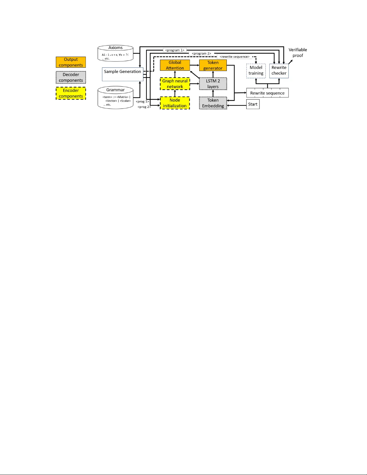
Equivalence of Dataow Graphs via Re write Rules Using a Graph-to-Sequence Neural Mo del Steve K ommrusch Colorado State University USA ste vek o@cs .colostate.edu Théo Barollet Inria France theo .barollet@inria.fr Louis-Noël Pouchet Colorado State University USA pouchet@colostate.edu Abstract In this work we target the pr oblem of provably computing the equivalence between two programs represented as dataow graphs. T o this end, we formalize the problem of equiva- lence between two programs as nding a set of semantics- preserving rewrite rules fr om one into the other , such that after the rewrite the two programs are structurally identi- cal, and therefore trivially equivalent. W e then dev elop the rst graph-to-sequence neural network system for program equivalence, trained to pr oduce such r ewrite sequences from a carefully crafted automatic example generation algorithm. W e extensiv ely evaluate our system on a rich multi-type linear algebra expression language , using arbitrary combi- nations of 100+ graph-rewriting axioms of equivalence. Our system outputs via inference a correct rewrite sequence for 96% of the 10,000 program pairs isolate d for testing, using 30- term programs. And in all cases, the validity of the sequence produced and therefore the provable assertion of program equivalence is computable, in negligible time. 1 Introduction The problem of pr ogram equivalence is summarized as de- termining whether two programs would always produce the same output for all possible inputs, and is a central problem in computing [ 19 , 27 , 48 ]. The problem ranges from undecid- able, e.g. [ 21 ], up to trivial in cases of testing the equivalence of a program with itself. W e claim the problem of program equivalence cannot be eciently mechanized by using a stochastic process to determine the equivalence between two program regions. Precisely , obtaining a binary answer yes/no to equivalence with a certain probability of condence does not lead to a provable conclusion on equivalence [ 54 ]. This is a major limitation to the deployment of machine learning techniques for pr ogram equivalence. Such an approach might prove use- ful for e.g. ltering, to focus via another process on only a subset of likely equivalent programs; but it is not a suitable approach for pro vably correct automated program equiva- lence checking as is typically developed, e.g., [ 3 , 28 , 36 ]. T o overcome the fundamental stochastic nature of neural networks, we use a ver y dierent approach to the pr oblem of pe-graph2seq , Februar y 2020, A rXiV 2020. machine learning for program equivalence: instead of mak- ing the network produce a binar y answer to the question of equivalence, we make the network produce a sequence of rewrite terms that make one program strictly equal to the other , if the input programs are equivalent . This way , the output of the network can be deterministically checked in negligible time. W e represent programs as graphs, and successively apply the axiom-based graph rewrites produced by the net- work on one of the input pr ograms, then ensure the resulting graph is identical to the other input graph via a simple si- multaneous depth-rst visit. Our neural network approach allows for deterministi- cally proving e quivalence, entirely avoids false p ositives, and quickly invalidates incorrect answers produced by the network (no deterministic answer is provided in this case). In a nutshell, we develop the rst graph-to-sequence neural network system to accelerate the search in the space of pos- sible combinations of transformation rules (i.e., axioms of equivalence in the input language) to make two programs/- graphs structurally identical without violating their original semantics. W e make the following contributions: • W e propose a machine learning system for program equiv- alence which ensures correctness for all non-equivalent pro- grams input, and a deterministically checkable output for equivalent programs. • W e introduce pe-graph2seq , the rst graph-to-seq- uence neural network system targeting program equivalence to the best of our kno wledge. W e pr ovide the rst implemen- tation of such graph-to-sequence systems in the p opular OpenNMT -py framework [ 29 ]. • W e present a complete implementation of our system oper- ating on a rich language for multi-type linear algebra e xpres- sions. Our system provides a correct rewrite rule sequence between two equivalent programs for 96% of the 10,000 test cases, for a typical inference time of 16ms per pair of pro- grams. The correctness of the rewrite rule is deterministically checkable in all cases in negligible time. The rest of the paper is organized as follo ws. Sec. 2 outlines the pr ogram equivalence problem we address, and motivates our proposed approach. Sec. 3 formally denes the type of program repr esentation and axioms of equivalence we ma- nipulate in this work, and formalizes the equivalence prob- lem addressed. A utomatic sample generation is discussed in Sec. 4 before Sec. 5 which introduces pe-graph2seq , its 1 pe-graph2seq, F ebr uar y 2020, ArXiV Ste ve K ommrusch, Théo Barollet, and Louis-Noël P ouchet ∗ 𝑎 + ∗ 1 𝑏 ∗ 1 𝑐 (a) 𝑎 ∗ ( 1 ∗ 𝑏 + 1 ∗ 𝑐 ) ∗ 𝑎 + 𝑏 𝑐 (b) 𝑎 ∗ ( 𝑏 + 𝑐 ) + ∗ 𝑎 𝑏 ∗ 𝑎 𝑐 (c) 𝑎 ∗ 𝑏 + 𝑎 ∗ 𝑐 + ∗ 𝑎 𝑐 ∗ 𝑎 𝑏 (d) 𝑎 ∗ 𝑐 + 𝑎 ∗ 𝑏 Figure 1. Examples of Computations overall design principles and key components. A complete experimental evaluation of our system is detailed in Sec. 6 . Related work is presented in Sec. 7 before concluding. 2 Motivation and O verview Input program representation Figs. 1a - 1d show four ex- amples of simple computations. For example, Fig. 1a models the expression 𝑎 ( 1 𝑏 + 1 𝑐 ) , one can imagine it to be the result of 𝑎 ( 𝑑 𝑏 + 𝑑 𝑐 ) after e.g. constant-pr opagation of 1 to 𝑑 . In the following we call these equivalently programs, sentences from a language, and graphs, the reader needs to be ready to jump between these e quivalent representations. They ar e dened by a single root, have nodes which can be opera- tions consuming the value of their immediate predecessor or terminal/input values, and a node produces a value that can be used by its immediate successors. In essence this is a classical dataow representation of the computation [ 14 ], and what our system uses as input program repr esentation. Rewrite rules as axioms of e quivalence Consider the programs in Fig. 1a versus Fig. 1b . The multiplication of a value by 1 does not change the value, if we rely on an axiom of equivalence stating 1 ∗ 𝑥 = 𝑥 , ∀ 𝑥 ∈ N . This ax- iom species a strict criterion of application: the node must be of type N , the expression pattern must b e 1 ∗ 𝑥 ; and a strict rewrite rule: replace a sub-graph 1 ∗ 𝑥 for any 𝑥 by the graph 𝑥 . In other words, replacing 1 ∗ 𝑏 by 𝑏 in Fig. 1a is a semantics-preserving re write, from the axiom of equivalence. In this work w e view the pr oblem of program equivalence as nding a sequence of semantics-preserving r ewrites, each from a precisely dened axiom of equivalence, that rewrites one program into the other . If one program can be rewritten by a sequence of individually-correct semantics-preserving transformations into another one, then not only are they equivalent under the set of axioms used, but the sequence forms the constructive and veriable proof of equivalence. A n example In this work we illustrate and experimentally evaluate our system using a rich linear algebra expr ession language because it exposes clearly (and intuitively) the various key concepts that must b e handle d: (1) operating on dataow graphs as input, supporting transformations that can (2) delete or (3) create new nodes in the graph, and transformations that (4) manipulate entire subtrees. W e also wanted a language with (5) multiple variable typ es, e.g. scalars, v ectors and matrices and (6) a large number of dier- ent operators with (7) distinct axioms applicable for each. All of these are captur ed in the language we experiment with, see Sec. 3 for its formal denition. When applying the axiom 𝐴 1 : 1 ∗ 𝑥 = 𝑥 , ∀ 𝑥 ∈ N on the program 𝑃 in Fig. 1a for its node 𝑏 , we obtain an equivalent and yet syntactically dierent program, we have 𝑃 ≡ 𝐴 1 ( 𝑏, 𝑃 ) . Applying the same axiom 𝐴 1 on 𝑐 in the re- sulting program leads to program 𝑃 ′ in Fig. 1b , and 𝑃 ′ ≡ 𝑃 ≡ 𝐴 1 ( 𝑐 , 𝐴 1 ( 𝑏, 𝑃 ) ) . Precisely , in graph terms, Fig. 1b is the result of a sequence of two semantics-preserving node deletion operations, as dened in the axiom. Consider now the axiom 𝐴 2 : 𝑥 ∗ ( 𝑦 + 𝑧 ) = 𝑥 ∗ 𝑦 + 𝑥 ∗ 𝑧, ∀ 𝑥 , 𝑦, 𝑧 ∈ N . This is the standard distributivity axiom on natural arithmetic. In terms of graph transformations, this is a complex rewrite: a new node is created ( ∗ ), one node is moved ( + to the root), and edges are signicantly modied. When this complex, but semantics-preserving, rewrite is applied to Fig. 1b , we obtain Fig. 1c , that is 𝑃 ≡ 𝐴 2 ( ∗ , 𝐴 1 ( 𝑐, 𝐴 1 ( 𝑏, 𝑃 ) ) ) . Finally consider the axiom 𝐴 3 : 𝑥 + 𝑦 = 𝑦 + 𝑥 , ∀ 𝑥 , 𝑦 ∈ N , the standard commutativity axiom for + . The graph transforma- tion does not change the number of nodes nor edges, instead only alters two specic edges. Note that as the previous ax- ioms, it also illustrates operations on sub-graphs: indeed 𝑥 and 𝑦 do not need to b e input/terminal nodes, they can be any subgraph producing a value of the proper typ e. This is illus- trated by applying on Fig. 1c to obtain Fig. 1d , that is the com- putation 𝑎𝑐 + 𝑎𝑏 . W e have 𝑃 ≡ 𝐴 3 ( + , 𝐴 2 ( ∗ , 𝐴 1 ( 𝑐 , 𝐴 1 ( 𝑏, 𝑃 ) ) ) ) , a veriable proof of equivalence under our axioms between the programs 𝑎 ( 1 𝑏 + 1 𝑐 ) and 𝑎𝑐 + 𝑎𝑏 , which involved struc- tural changes including no de deletion, creation and edge modication. Note the bidirectional nature of the process: one can rewrite from 𝑎 ( 1 𝑏 + 1 𝑐 ) to 𝑎𝑐 + 𝑎𝑏 , or the con- verse using the same (but rev erted) se quence. Note also the non-unicity of a sequence: by possibly many ways a program can be rewritten into another one, for example the sequence 𝑃 ≡ 𝐴 3 ( + , 𝐴 1 ( 𝑐 , 𝐴 1 ( 𝑏, 𝐴 2 ( ∗ , 𝑃 ) ) also correctly rewrites Fig. 1a into Fig. 1d . Conv ersely , a sequence may not exist: for example no sequence of the 3 above axioms allow to rewrite 𝑎 + 𝑏 into 𝑎 ∗ 𝑏 . W e call these non-equivalent in our system, that is precisely if there is no sequence of axioms that can be applied to rewrite one program into the other . 2 Equivalence of Dataflo w Graphs Using Graph-to-Sequence Model pe-graph2seq, F ebr uar y 2020, ArXiV The ne ed for a veriable procedure A key motivation of our work is to enable in a safe and provably corr ect way the use of machine learning for program equivalence. For full automation of the process, we focus on ensuring correctness in case an equivalence result is compute d by the system. That is, our system by design answers only with a probability of condence that the two programs are not equivalent, but it produces a v eriable procedure to assess equivalence other wise. W e believe such an approach is key for a practical, automated deployment of neural networks for program equivalence: veriably proving equivalence to ensure no false positive, while tolerating a moderate amount of false negative (i.e., missing that two programs wer e in fact equivalent). Numerous practical applications of the kind of system we develop exist, even on the linear algebra language we demon- strate on: for example the automatic correction of exercises for students, wher e they typically need to pr ove equivalence between two formulas by successive application of other formulas/axioms. Languages like e.g. Matlab could use inter- active checking of the equivalence between the expression being typed and the pre-existing library implementations (e .g., BLAS-based [ 22 ]) to use instead accelerated implemen- tations when possible in real-time. But we have designed and evaluated our system in a robust enough way to be ap- plicable to a wide variety of languages and problems, as long as they can be cast in the framework in Sec. 3 . W e discuss other uses cases and applications in Sec. 6 . The space of equivalences Intuitively , our approach to program e quivalence is as follows. W e can intelle ctually reason on a graph for equivalent programs where each node represents a distinct program in the language, and two no des (i.e., two dierent programs) are connected by a directed edge i the source node can b e rewritten as the target node by the application of a single one of the pre-dened axioms for equivalence. The edge is labeled by the axiom used and the specic p osition in the source node’s program to wher e it needs to b e applied to obtain the program in the target node. Then there will b e one or more paths in this graph from the two nodes modeling the two input programs if they are equivalent ( one can be rewritten into the other while preserving semantics); and no path if no such rewrite is possible, that is the programs would be not equivalent in our framework. Exposing a path between two nodes is sucient to prove the equivalence of their associated programs. This path is exactly a sequence of rewrite rules from one program to another . T o test the corr ectness of an arbitrary sequence, i.e., verify if this path exists in the graph and assess equivalence if it does, one then ne eds to simply apply the proposed sequence to one of the input programs: verify at each step that the rewrite in the sequence is indee d appli- cable (by a simple check of the applicability of the axiom at this particular program point), and eventually ensure the rewritten pr ogram is identical to the other input one. This test can be computed in time mostly linear with the pr ogram size in our framework, and when successful it implements a constructive proof of equivalence between the tw o pr ograms. Pathnding equivalence proofs When formulating the program equivalence problem this way , we can then view its solution as learning how to build at least one feasible path b etween any two pairs of nodes in the above graph, when it can exist. W e can see that by design, there is a lot of redundancy in this space: the same labeled path will occur between many dierent pairs of programs (e.g., those where only the variable symbols dier), and there are typically many paths between the same two (equivalent) programs. This creates opportunities for the system to learn program representation and path construction techniques more easily . Our key contribution is the development of a deep learn- ing framework that learns this procedure automatically . The neural network system we build is trained by randomly sam- pling this graph, with samples made of two nodes and a path between them when training on equivalent programs, and an empty path otherwise. W e specically learn a generalization of the problem of nding paths in this graph as follows. W e represent input programs in a carefully-crafted normalized dataow-like graph encoded as a gated graph neural net- work [ 11 , 44 ], to enable structural, size-tolerant reasoning by the network on the inputs. It is combined with a global attention-based mechanism and a memory-based LSTM [ 24 ] decoder which can memorize graph changes for producing the r ewrite se quence and enable path-size tolerant reasoning, while following the properties of the axioms for equivalence. In a nutshell, we make the network learn a stochastic ap- proximation of an iterative algorithm that would be able to construct a feasible path ( when possible) between any two pairs of nodes in this equivalence graph, but trained simply by randomly sampling pairs of nodes and one carefully la- beled path between them. This avoids entirely the need to craft smart exploration heuristics to make this path-nding problem feasible in practice. This is instead what we let the neural netw ork learn automatically; and specically why we implemented graph neural networks to solve this problem [ 44 , 54 ]. W e rely on the network to suggest a transformation path by inference, and then verify its validity in linear time. System overview In order to implement our approach, we need a simple-enough grammar for a language, in which we enumerate randomly valid sentences, and a set of axioms of equivalence between two sentential forms expressible as semantics-preserving re write rules from one to the other . The system takes as input two pr ograms (i.e., sentences ac- cepted by the language), and produces an ordered sequence of axioms along with their position of application (or node) that can be used to rewrite sequentially one input program into the other input pr ogram. This sequence is then checked for correctness using the axioms as reference. T o train the 3 pe-graph2seq, F ebr uar y 2020, ArXiV Ste ve K ommrusch, Théo Barollet, and Louis-Noël P ouchet Figure 2. pe-graph2seq System O verview system, we generate pairs of equivalent programs by iter- ating the axioms with random probability on one program, thereby generating both a path to equivalence and the target program. Random programs ar e generated so as to respect the grammar dened. The training set is then appropriately selected from these random samples, as detailed in Sec. 6 . When the system outputs that two programs ar e equiva- lent, as provable reasoning (the re write sequence) is always produced, no false positive can ever occur . When the system fails to demonstrate equivalence, no provable conclusion is produced regarding the input programs ho wever: we are left with only a (high) probability of non-equivalence. A key of our approach is to introduce graph-to-sequence neural networks to quickly compute one or more possible rewrite sequences. The details of the network are covered in Sec. 5 . In a nutshell, the key principle is to combine a memory-based neural network approach, e.g., using Long- Short T erm Memory (LSTM) [ 24 ] neurons and a graph neural network design ( which uses Gated Recurrent Units (GRUs) internally) [ 11 ] that matches our program graph representa- tion. W e use a sequence generation principle , using an atten- tion mechanism to allow observation of program graph node information while generating the rewrite sequence. This en- ables the production of the re write sequence token-by-token, matching our axiom of equivalence design principle. As presented in Sec. 5 , we designed an ecient emb ed- ding of the program equivalence problem into a graph neural network ( Node initialization ) to facilitate the network’s abil- ity to walk the program graphs and memorize structural changes being made by applying the axioms. T o the best of our knowledge, this is the rst graph-to-sequence system for program equivalence, which outputs veriable proofs. Our system is fully implemented end-to-end in OpenNMT - py and is ready for artifact evaluation. A s detaile d in Sec. 4 we developed a very rigorous evaluation (test) set to ensure our system has developed some intelligence, which is fully conrmed in Sec. 6 . As an extreme case, even if we would make a system that each time two programs are checked for equivalence, produces systematically all possible distinct rewrite sequences it has ever se en during training (up to 118k in our experiments), and we check all of these outputs for correctness and applicability for the input programs, this would still not e xceed 60% of correct test cases for equivalent programs tested. W e report a steady 95% or more using only a beam size of 10, that is asking the network to output only the 10 most likely rewrite sequences for the input programs. 3 Framework for Program Equivalence W e now present the formalism we use in this work to rep- resent programs and their equivalences. W e carefully co- designed this problem representation and the (graph) neural network approach to make the best use of machine learning via deep networks, as discussed in Sec. 5 . 3.1 Program Representation A key design aspect is to match the capability of the neural network to model the input as a walkable graph with the actual input pr ogram repr esentation to be handled. W e there- fore model programs in a datao w-like representation (i.e ., a directed graph), using a single root/output node. In par- ticular , we do not restrict to tr ee-like structures nor acyclic graphs, as briey discussed in Sec. 6.4 . Denition 3.1 (Program graph node) . A node 𝑛 ∈ 𝑁 in the program graph models n-ary operations and input operands. A node produces a value which can be consumed by any of its immediate successors in the graph. When a node has no predecessor , it models an input value. The output value for the computation is produced by the unique root node 𝑛 𝑟 𝑜 𝑜 𝑡 of the graph, the only node without successor . Denition 3.2 (Program graph directed edge) . A directed edge 𝑒 𝑛 1 ,𝑛 2 : 𝑛 1 → 𝑛 2 with 𝑛 1 , 𝑛 2 ∈ 𝑁 in the program graph connects the producer of a value ( 𝑛 1 ) to a node consuming this value in the computation. Denition 3.3 (Program graph) . A program graph 𝐺 is a directed dataow graph modeling the computation, made of nodes 𝑛 𝑖 ∈ 𝑁 and edges 𝑒 𝑛 𝑖 ,𝑛 𝑗 ∈ 𝐸 as dened in Def. 3.1 and Def. 3.2 . That is, 𝐺 = ⟨ 𝑛 𝑟 𝑜 𝑜 𝑡 , 𝑁 , 𝐸 ⟩ . Ther e is no dangling edge nor unconnected node in 𝐺 . Language of linear algebra expressions W e dev eloped a complex-enough language to evaluate carefully our work, 4 Equivalence of Dataflo w Graphs Using Graph-to-Sequence Model pe-graph2seq, F ebr uar y 2020, ArXiV that captures rich linear algebra expr essions. Specically , we support 3 types of data/variables in the program: scalars, vectors and matrices. W e use the standard notation 𝑎, ® 𝑎, 𝐴 for scalars, vectors and matrices. W e evaluate using dierent variable names for each of the 3 types above, along with their identity and absorbing elements. W e also model a rich set of operators, mixing dierent unary and binar y operations for each type. Specically , we support ∗ 𝑠 , + 𝑠 , − 𝑠 , / 𝑠 between scalar operands, and + 𝑣 , − 𝑣 , ∗ 𝑣 between vectors and + 𝑚 , − 𝑚 , ∗ 𝑚 for matrices. For − , / we also support their unar y version for all types, e.g. − 1 𝑠 for unary scalar inversion and − 𝑢𝑚 for unary matrix negation. For example 𝑎 − 1 𝑠 computes to 1 / 𝑎 . W e also support multi- type operations, such as vector and matrix scaling by a scalar ∗ 𝑠 𝑣 , ∗ 𝑠𝑚 . W e support two specic unar y matrix op erations, transpose 𝑡 𝑚 and matrix inversion as − 1 𝑚 . Note every opera- tor has a unique name in our language , driven by the type of its operand. This will facilitate the learning of the program embedding, avoiding the need to learn typ e propagation. Examples Programs of the form 𝐴 ( 𝐵𝐶 𝑡 𝐷 ) 𝐸 − 1 , ® 𝑎 + 𝑏 ® 𝑐 − 1 − 0 ® 𝑒 , ( 𝑎 + 𝑏 ) + ( 𝑐 ( 𝑑 / 𝑒 ) ) , ( 𝑎𝐴 + 𝑏 𝐵 ) 𝐶 𝑡 etc. can be parsed trivially to our representation, one simply needs to b e able to provide a unique name for each operand and operator type (possibly via some analysis, or simple language design principles), that is avoiding to ov erload the semantics of operators and operands. Note the semantics is never e xplicitly provided to our DNN approach, it is learned by examples. There will be no example of the form e.g. 𝑎 + 𝐴 , an invalid program in our language. W e b elieve a sensible approach is to dev elop a clean, reg- ular grammar for the language to be handled, as implicitly these are concepts the DNN will ne ed to learn. W e did so, using a classical LL(1) grammar description of our linear algebra language. This is not a requirement of our approach, as one can arrive to the desired input program graph by any means necessary , but we believe making the r easoning on the language structure “ easy” is an important design aspe ct. 3.2 Axioms of Equivalence A central aspect of our approach is to view the pr oblem of program equivalence as nding a sequence of locally-correct rewrite rules that each preserve the semantics, thereby mak- ing incremental reasoning p ossible . W e explicitly do not con- sider non-semantics-preserving axioms. A rich structure of alternate but equivalent ways to rewrite one program to an- other makes the problem easier to sample and more amenable to machine learning. Semantics-preserving axioms enable incremental per-axiom reasoning, and enforce semantics preservation without overly complicated semantics analysis; while still manipulating a v ery rich space of transformations. T o illustrate this we specically design axioms that perform complex graph modications, such as node deletion or cre- ation, subtree manipulation, multi-node graph changes, etc. A graph pattern can be viewed as a pattern-matching rule on graphs and its precise applicability criteria. It can also be viewed as a sentential form of the language grammar , e.g. ScalarVal PlusOp ScalarVal is a pattern, if the grammar is well formed. Denition 3.4 (Graph pattern) . A graph pattern 𝑃 is an un- ambiguous structural description of a (sub-)graph 𝐺 𝑃 , which can be deterministically matched in any program graph 𝐺 . W e have 𝑃 = ⟨ 𝐺 𝑃 , 𝑀 𝑛 , 𝑀 𝑒 ⟩ where for each node 𝑛 𝑖 ∈ 𝑁 𝐺 𝑃 , { 𝑛 𝑚𝑎𝑡 𝑐 ℎ } = 𝑀 𝑛 ( 𝑛 𝑖 ) returns the set of node values 𝑛 𝑚𝑎𝑡 𝑐 ℎ accepted to match 𝑛 𝑖 on a graph 𝐺 . For 𝑛 𝑖 , 𝑛 𝑗 ∈ 𝑁 𝐺 𝑃 , 𝑒 𝑖 = 𝑀 𝑒 ( 𝑛 𝑖 , 𝑛 𝑗 ) returns the set of edges between 𝑀 ( 𝑛 𝑖 ) and 𝑀 ( 𝑛 𝑗 ) to be matched in 𝐺 . A pattern 𝐺 𝑃 is matched in 𝐺 if ( a) ∀ 𝑛 𝑖 ∈ 𝐺 𝑝 , ∃ 𝑛 𝑚 = 𝑀 ( 𝑛 𝑖 ) ∈ 𝑁 𝐺 ; (b) ∀ 𝑒 𝑖 ∈ 𝐸 𝐺 𝑃 , ∃ 𝑒 𝑀 𝑛 ( 𝑛 𝑖 ) ,𝑀 𝑛 ( 𝑛 𝑗 ) = 𝑀 𝑒 ( 𝑛 𝑖 , 𝑛 𝑗 ) ∈ 𝐸 𝐺 ; and (c)  𝑒 𝑀 𝑛 ( 𝑛 𝑖 ) ,𝑀 𝑛 ( 𝑛 𝑗 ) ∈ 𝐸 𝐺 ≠ 𝑀 𝑒 ( 𝑛 𝑖 , 𝑛 𝑗 ) . Note when a graph pattern models a rewrite, 𝑀 𝑛 and 𝑀 𝑒 are adjusted accordingly to output the rewrite of a no de 𝑛 ∈ 𝑁 𝐺 into its desir ed value , instead of the set of acceptable nodes from 𝑛 ∈ 𝑁 𝐺 𝑃 . Denition 3.5 (Axiom of equivalence) . An axiom 𝐴 is a semantics-preserving rewrite rule 𝐺 ′ = 𝐴 ( 𝑛, 𝐺 ) that can ar- bitrarily modify a program graph 𝐺 , and produces another program graph 𝐺 ′ respecting Def. 3.3 with identical seman- tics to 𝐺 . W e note 𝐴 : ⟨ 𝑃 𝑚𝑎𝑡 𝑐 ℎ , 𝑃 𝑟 𝑒 𝑝𝑙 𝑎𝑐𝑒 ⟩ an axiom, where 𝑃 𝑚𝑎𝑡 𝑐 ℎ , 𝑃 𝑟 𝑒 𝑝𝑙 𝑎𝑐𝑒 are graph patterns as per Def. 3.4 . The appli- cation of axiom 𝐴 to no de 𝑛 in 𝐺 is written 𝐴 ( 𝑛, 𝐺 ) . W e can compose axioms to form a complex rewrite se- quence. Denition 3.6 (Semantics-preserving axiom composition) . Given a sequence 𝑆 : 𝐴 1 ( 𝑛 1 , 𝐴 2 ( 𝑛 2 , . .., 𝐴 𝑚 ( 𝑛 𝑚 , 𝐺 ) ) ) of 𝑚 ax- ioms applications. It is a semantics-preserving composition if for each 𝐺 𝑗 = 𝐴 𝑖 ( 𝑛 𝑖 , 𝐺 𝑖 ) ∈ 𝑆 , 𝑃 𝐴 𝑖 𝑚𝑎𝑡 𝑐 ℎ succeeds on the sub- graph with root 𝑛 𝑖 in 𝐺 𝑖 , and 𝐺 𝑗 is obtained by applying 𝑃 𝐴 𝑖 𝑟 𝑒 𝑝𝑙 𝑎𝑐𝑒 to 𝑛 𝑖 . Theorem 3.7 (Program graph e quivalence) . Given a pro- gram 𝐺 . If 𝐺 ′ = 𝑆 ( 𝐺 ) such that 𝑆 is a semantics-preserving sequence as per Def. 3.6 , then 𝐺 ≡ 𝐺 ′ , they are equivalent under the axiom system used in 𝑆 . This is a direct conse quence of using only semantics- preserving axioms, each rewrite cannot individually alter the semantics, so such incremental composition does not. It leads to the formal problem we are addr essing: Corollary 3.8 (Program graphs e quivalence matching) . Given two programs 𝐺 , 𝐺 ′ . If there exist a semantics-preserving se- quence 𝑆 such that 𝐺 ′ = 𝑆 ( 𝐺 ) , then 𝐺 ≡ 𝐺 ′ . Note here = means complete structural equivalence be- tween the two graphs: they are identical in structure and label/node values. Determining 𝐺 = 𝐺 ′ amounts to visiting both graphs simultaneously e.g. in depth-rst search fr om 5 pe-graph2seq, F ebr uar y 2020, ArXiV Ste ve K ommrusch, Théo Barollet, and Louis-Noël P ouchet the root to ensure structural equivalence, and also verifying the same node labels appear in both at the same time. This is trivally implemented in linear time in the graph size. Language of linear algebra expressions W e have imple- mented a total of 102 dierent axioms for our language, made of the multi-type versions of the 13 core restructuring axioms described later in T able 1 . They all follow established linear algebra properties. Note dierent data types have dier ent axioms following typical linear algebra rules, e.g., matrix- multiplication does not commute, but scalar and vector mul- tiplications do. Examples of axioms include 𝑥 ( 𝑦𝑧 ) → ( 𝑥 𝑦 ) 𝑧 , 𝑋 − 𝑋 → 𝑂 , − ( ® 𝑥 − ® 𝑦 ) → ® 𝑦 − ® 𝑥 , or 𝑋 𝑡 𝑡 → 𝑋 , an exhaustive list is displayed in the Supplementary Material. In our e xperiments, we pr esume matrix and vector dimen- sions are appropriate for the given operation. Such dimen- sion compatibility checks are simple to implement by e.g. introducing additional nodes in the program representation, but are not considered in our test language. Examples W e illustrate axiom-based rewrites using ax- ioms presented in later T able 1 . Note axiom names follow the structural changes applied. For example , w e have 𝑎 + 𝑏 ≡ 𝑏 + 𝑎 : { 𝑎 + 𝑏 } = 𝐶 𝑜 𝑚 𝑚 𝑢 𝑡 𝑒 ( { +} , { 𝑏 + 𝑎 } ) . 𝑎 + 𝑏 + 𝑐 ≡ 𝑏 + 𝑐 + 𝑎 : { 𝑎 + 𝑏 + 𝑐 } = 𝐶 𝑜𝑚𝑚 𝑢𝑡 𝑒 ( {+ 1 } , 𝐶 𝑜𝑚𝑚 𝑢𝑡 𝑒 ( { + 2 } , { 𝑏 + 𝑐 + 𝑎 }) . Note we refer to dierent nodes with the same symbol (e.g., + 2 ) subscripting them by their order in a DFS traversal of the program graph, starting from the unique root. W e have 0 ≡ 𝑎 − 𝑎 : { 0 } = 𝐶 𝑎𝑛𝑐𝑒 𝑙 ( {− } , { 𝑎 − 𝑎 } ) . These can b e com- bined in comple x paths, e.g., 𝑏 + 𝑐 ≡ 𝑐 + 𝑏 + ( 𝑎 − 𝑎 ) : { 𝑏 + 𝑐 } = 𝐶 𝑜𝑚𝑚 𝑢 𝑡 𝑒 ( { + } , 𝑁 𝑜 𝑜 𝑝 ( { + } , 𝐶 𝑎𝑛𝑐 𝑒 𝑙 ( {− } , { 𝑐 + 𝑏 + ( 𝑎 − 𝑎 ) }) ) ) . Such axioms are developed for scalars, matrices and vectors, and include complex re writes such as distributivity rules and transpositions. A total of 102 axioms are used in our system. 3.3 Space of Equivalences W e now dene the search space being explored in this work, i.e., the exact space of solutions on which the DNN system formally operates, and that we sample for training. Denition 3.9 (Graph of the space of e quivalences) . Given a language L . The directed graph of equivalences between programs is 𝐺 𝑒𝑞𝑢𝑖 𝑣 = ⟨ 𝑁 𝑒𝑞𝑢𝑖 𝑣 , 𝐸 𝑒𝑞𝑢𝑖 𝑣 ⟩ such that ∀ 𝑙 ∈ L , 𝑛 𝑙 ∈ 𝑁 𝑒𝑞𝑢𝑖 𝑣 , and 𝑒 𝐴 𝑖 ,𝑥 𝑛 𝑖 ,𝑛 𝑗 : 𝑛 𝑖 → 𝑛 𝑗 ∈ 𝐸 𝑒𝑞𝑢𝑖 𝑣 i 𝑛 𝑗 ≡ 𝐴 𝑖 ( 𝑥 , 𝑛 𝑖 ) , ∀ 𝐴 𝑖 in the axiom system and 𝑥 a position in 𝑛 𝑖 where 𝐴 𝑖 is applicable. In other words, the graph has one node per possible pro- gram in the language L , and a single axiom application leads to connecting two nodes. W e immediately note that 𝐺 𝑒𝑞𝑢𝑖 𝑣 is a (possibly innite) multigraph, and contains circuits. Theorem 3.10 (Program e quivalence with pathnding) . Given two programs 𝑛 𝑖 , 𝑛 𝑗 ∈ 𝑁 𝑒𝑞𝑢𝑖 𝑣 . If there is any path from 𝑛 𝑖 to 𝑛 𝑗 in 𝐺 𝑒𝑞𝑢𝑖 𝑣 , then 𝑛 𝑖 ≡ 𝑛 𝑗 . The proof is a direct consequence of Def. 3.9 . In this work, we randomly sample this exact graph to learn how to build paths b etween arbitrar y programs. As it is a multigraph, there will be possibly many dierent sequences modeled to prove the equivalence between two programs. It is sucient to expose one to prove equivalence . Corollary 3.11 (Semantics-preserving rewrite se quence) . A ny directed path in 𝐺 𝑒𝑞𝑢𝑖 𝑣 is a semantics-preserving rewrite sequence between the programs, described by the se quence of axioms and program p osition lab eling the edges in this path. This sequence forms the proof of e quivalence. W e believe that ensuring there are possibly (usually ) many ways to compute a pr oof of e quivalence in our specic frame- work is key to enable the DNN approach to learn automat- ically the pathnding algorithm for building such proofs. Other more compact representations of this space of equiv- alences are clearly possible, including by folding no des in the equivalence graph for structurally-similar programs and folding equivalent paths b etween nodes. When building e.g. a deterministic algorithm for pathnding, such space size reduction would bring complexity benets [ 9 , 27 ]. W e be- lieve that for the ecient deployment of graph-to-sequence systems, exposing signicant redundancy in the space fa- cilitates the learning process. W e also alleviate the need to reason on the properties of this space to nd an ecient traversal heuristic. 4 Samples Generation Following the problem formalization in Sec. 3 , the next chal- lenge is to automatically sample the search space graph. The careful design of this step is key: as w e let the DNN learn by example only what the axioms are and when they are appli- cable, along with what is the general structure of a program, we must car efully sample the space of e quivalences to ensure appropriate distributions of the examples. W e produce a nal dataset of 420,000 tuples ( 𝑃 1 , 𝑃 2 , 𝑆 ) , a pair of input programs and a possible rewrite sequence between them. W e outline below its generation principles, extensive details and the algorithms used are presented in Supplementary Material. 4.1 Random Sample Generation Deep learning typically requires large training sets to b e eectively deployed, our system is no exception. Hence the need to automate the generation of an arbitrary number of samples. With this pr ocess, w e can cr eate as large and varied a dataset as our machine learning approach requires. W e specically use randomized program generation al- gorithms that are inspired by a given language grammar . While using a grammar as input is not required, the b ene- ts are immediate in particular for regular LL(1) languages: one can build random parse trees by simply iterating the grammar , randomly choosing b etween possible productions. 6 Equivalence of Dataflo w Graphs Using Graph-to-Sequence Model pe-graph2seq, F ebr uar y 2020, ArXiV The leaves obtained will form a sentence accepte d by the language, i.e., a pr ogram [ 13 ]. In particular , we skew the pseudo-random generation so that (1) binary operations are more likely to be created than unary operations, and (2) the initial probability that a child of the created graph no de will itself be an operation (as opposed to a terminal symbol) is set to 91%. The algorithm then sub- tracts a 23% probability for children at each level of the graph, so that the path length from the root to any leaf do es not exceed 6. Note these probabilities and algorithm have been computed to match the size restrictions for our system eval- uated in Sec. 6 : handle programs with 30 nodes maximum, and sequences made of 5 axiom applications maximum. W e produce equivalent program samples by iterating pseudo- randomly the axioms on one randomly generated program to produce a rewrite sequence and the asso ciated equivalent program. The process iterates through all nodes of a pro- gram graph, and at each no de checks which axiom(s) can b e applied. E.g., the + 𝑚 operator can have the Commute axiom applied, or depending on subtrees it may be allowed to have the Factorleft axiom applie d, as discussed in Se c. 6 . Generally we choose to apply or not an operator with 50% probability , so that pe-graph2seq is forced to rely on analysis of the two programs to determine whether an operator is applied instead of learning a bias due to the local node features. 4.2 Final Experimental Dataset After these generation algorithms ar e run, a nal data prepa- ration process is done to prune the dataset for the learning phase. Any lexically equivalent program pair (if any ) is re- moved. Importantly , we remove some cases with only 1 or 2 axioms being used once, to slightly bias the dataset to longer rewrite sequences. W e also ensured a reasonable statistical distribution of the use of the various axioms. Rewrite Rule Example(s) Samples using rule Cancel (A - A ) → O, (b/b) → 1 13.0% Noop (v - o) → v 29.2% Double 𝐴 𝑡 𝑡 → 𝐴 , 1/1/x → x 7.5% Commute (a + b) → (b + a) 29.5% DistributeLeft (a + b)c → ac + bc 28.0% DistributeRight a(b + c) → ab + ac 19.6% FactorLeft ab + ac → a(b+c) 2.1% FactorRight ac + bc → (a+b)c 3.1% AssociativeLeft a(bc) → (ab)c 16.6% AssociativeRight (ab)c → a(bc) 16.2% FlipLeft -(v - w ) → w-v 9.7% FlipRight a/(b/c) → a(c/b) 23.2% Transpose ( 𝐴𝐵 ) 𝑡 → 𝐵 𝑡 𝐴 𝑡 , 10.1% T able 1. Distribution of the set of 13 rewrite rule types in the nal dataset. The totals add to more than 100% since a single program pair can require multiple rewrite rules for equivalence proof. In total, 102 axioms are used, when considering dierent data types and operators. T able 1 details the distribution of rewrite rules in the dataset we created, we categorized the axioms by the struc- tural graph changes they implement. Note specically for our experiments in Sec. 6 , as we target program graphs made of 30 nodes maximum and sequences using a maximum of 5 axioms applications, we prune fr om the set any entry that does not t these restrictions. The full dataset is then split into training, validation and test sets is discussed in Se c. 6.1 . 5 Deep Neural Networks for Program Equivalence Prior work explored using graph neural networks (GNNs [ 33 ]) to nd a program embedding usable for machine learn- ing, e.g., [ 5 ], GNNs for binar y code equivalence checking, e.g., [ 54 ], as well as using a graph-to-sequence model with attention to analyze and generate human language, e.g., [ 11 ]. But to the b est of our knowledge, our work is the rst to use a graph-to-sequence approach to generate a veriable rewrite rule sequence which prov es two program graphs ar e equivalent. In this section we discuss the implementation details of these components. 5.1 pe-graph2seq Deep Neural Network Fig. 2 overviews the entire system architecture including sample generation, the pe-graph2seq network, and the rewrite checker . Ke y design decisions are presented below . System components The system in Fig. 2 is composed of the following blocks. Node initialization is the process in which the program graph is used to initialize the data struc- tures used by the neural network with correct values, it is a direct procedure which sets up the network. Graph neural network refers to a neural network that has weights which allo w it to learn interr elations between network nodes based on edge connections for the problem set it is trained on. Global attention [ 35 ] when used with a graph neural net- work allows the decoder to pay attention to certain nodes in the graph as it creates each token in the output sequence. For example, a node associated with scalar multiply might get extra attention when deciding that the axiom to apply is commutation. T ok en embedding is a neural network layer in which tokens are assigned a learnable multidimensional embedding vector [ 37 ] which can then b e processed by other neural network components. LSTM 2 la yers is referring to 2 layers of Long Short T erm Memory (LSTM) neurons, each layer can have hundreds of neurons. An LSTM has ’long’ memory in the sense that weights which dene its behavior are learned from the train- ing data so it has a long memory regarding all the training data it has seen. It has a ’short’ memory in the sense that it is a recurrent neural netw ork unit which can change state as the network processes output tokens. As such, a given 7 pe-graph2seq, F ebr uar y 2020, ArXiV Ste ve K ommrusch, Théo Barollet, and Louis-Noël P ouchet LSTM cell could change state when the Commute token is output so that the Commute axiom is not repeated. T ok en generator is the nal output portion of the network. It learns to output the correct token base d on the current LSTM hidden states and the global attention from the graph neural network. As each token is output, it feeds back into the LSTM layer through the emb edding layer to aect the next state of the LSTM. Graph neural network internal representation The sam- ple generation discussed in section A.1 pro vides input to the Node Initialization module in Fig. 2 to create the initial state of our graph neural network. For each node in the program graph, a node will be initialized in our graph neural network. Each node has a hidden state represented by a vector of oating point values which are used to create an embedding for the full meaning of the given node. Initially all of the dimensions of the hidden states of the nodes are set to zero except for 2. Given 𝑁 tokens in our input program language, one of the dimensions from 1 through 𝑁 of a node will be set based on the token at the program position that the node represents. For e xample, if the scalar variable 𝑎 is assigned to be token 3 in our language, then the 𝑎 node in Fig. ?? would be initialized to 1.0. This is a one-hot encoding similar to that used in neural machine translation models [ ? ]. The second non-zero dimension in our node initialization indicates the tree depth, with the root for the program being at depth 1. W e set the dimension 𝑁 + 𝑑 𝑒 𝑝 𝑡 ℎ to 1.0; hence, the 𝑎 node in Fig ?? , which is at level 2 in the graph, would set dimension 𝑁 + 2 to 1. In addition to nodes correlating to all tokens in both input programs, we initialize a root node for program comparison which has edges connecting to the root nodes of both programs. The root node does not represent a token from the language, but it is initialized with a 1.0 in a hidden state dimension reserved for its identication. For a graph neural netw ork, the edge connections between nodes are a crucial part of the setup. In particular , to match the formulation of our problem, we must ease the ability of the network to walk the input program graphs. W e therefor e designed a unied graph input, where both program graphs are unied in a single graph using a single connecting root node; and where additional edges are inserted to make the graph fully walkable. In our full model, we support 9 edge types and their re- verse edges. The edge typ es are: 1) left child of binar y op, 2) right child of binary op, 3) child of unar y op, 4) root node to program 1, 5) root node to program 2, 6-9) there are 4 edge types for the four node grandchilden (LL, LR, RL, RR). After the node hidden states and e dge adjacency matrix are initialized, the network is ready to begin processing. This initial state is indicated in gure 3 by the solid circles in the lower left of the diagram. The combination of the root node type and the edges con- necting it to programs 1 and 2 allow the network to learn weights which allow the graph neural network to ’walk’ in- formation from the graph of program 1 through the root node to the graph of program 2 as it creates the node embed- dings necessary for rewrite rule generation. This is a novel feature of our network not used in prior work with GNNs on program analysis [ 5 , 54 ]. Graph neural network processing After initialization, the graph neural network iterates in order to convert the initial node state into the emb eddings nee ded for rewrite rule gen- eration. For our problem size , we iterate the GNN 10 times. This process is shown in gure 3 with the dotted circles starting with the initial state on the bottom left and rising to the nal state b efore input to the LSTM-based deco der . Given an initial hidden state for node 𝑛 of 𝑥 𝑛 ( 0 ) , 𝑥 𝑛 ( 𝑡 + 1 ) is computed with a learnable function 𝑓 which combines the current hidden state 𝑥 𝑛 ( 0 ) , the edge types 𝑙 𝑖𝑛 [ 𝑛 ] of edges entering node 𝑛 , the edge types 𝑙 𝑜𝑢 𝑡 [ 𝑛 ] of edges exiting node 𝑛 , and the hidden states 𝑥 𝑛𝑒 [ 𝑛 ] of the neighbors of node 𝑛 : 𝑥 𝑛 ( 𝑡 + 1 ) = 𝑓 ( 𝑥 𝑛 ( 𝑡 ) , 𝑙 𝑖𝑛 [ 𝑛 ] , 𝑥 𝑛𝑒 [ 𝑛 ] ( 𝑡 ) , 𝑙 𝑜𝑢 𝑡 [ 𝑛 ] ) Each of the edge types has a dier ent weight matrix for learning, allowing aggregation of information into a giv en node related to its position and function in the full graph of the program. The root node initial state along with the special edge types connecting it to the graph trees of the programs are able to learn spe cic information regarding rewrite rules as demonstrated by our experimental results. Graph neural network output to decoder Fig. 3 shows two ways that the nal node values for the graph are used by the decoder to create the r ewrite rules. First, the nal root node value 𝑥 𝑟 𝑜 𝑜 𝑡 ( 10 ) is fed through a learnable bridge func- tion to initialize the 2 lay er LSTM of the decoder network. In this way , the aggregated information of the 2 programs see ds the generation of the rewrite rules. The LSTM layer updates as each output token 𝑦 𝑗 is generated with a learnable func- tion based on the current decoder hidden state ℎ 𝑑 𝑗 at decoder step 𝑗 and the previous output token 𝑦 𝑗 − 1 [ 16 ]. Second, all nodes in the graph can be used by a learnable attention lay er [ 7 ]. The attention layer creates a context vector 𝑐 𝑗 which can be used by a learnable function 𝑔 when computing the probability for generating the 𝑗 th output token 𝑃 ( 𝑦 𝑗 ) : 𝑃 ( 𝑦 𝑗 | 𝑦 𝑗 − 1 , 𝑦 𝑗 − 2 , . .., 𝑦 0 , 𝑐 𝑗 ) = 𝑔 ( ℎ 𝑑 𝑗 , 𝑦 𝑗 − 1 , 𝑐 𝑗 ) (1) By using the root node only for seeding the initial hidden state ℎ 𝑑 0 of the decoder , that node and the w eights associated with the conne ctions to the program graphs for programs 1 and 2 are congured so that they learn the information necessary for starting o the rewrite rule sequences. In par- allel, after the graph neural network iterations complete, the nal embedding for all the nodes in the graphs for programs 1 and 2 are only used by the attention network, so their - nal embedding learns to provide useful information during 8 Equivalence of Dataflo w Graphs Using Graph-to-Sequence Model pe-graph2seq, F ebr uar y 2020, ArXiV the rewrite rule generation (i.e., after initialization of the decoder). Figure 3. Graph-to-sequence neural network data ow de- tails. Beam search A typical approach when using sequence- to-sequence systems is to enable beam search , the process of asking for multiple answ ers to the same question to the network. It is particularly relevant when creating outputs which can be automatically checked [ 2 , 16 ]. Beam search can be viewed as proposing multiple possible paths/rewrite sequences. Given the stochastic nature of generation model, a beam width of 𝑛 can be thought of as creating the 𝑛 most likely sequences given the training data the mo del as learned on. Each proposal can be checked for validity , the rst valid one is outputted by the system, demonstrating equivalence. If no sequence is valid, the system answers the programs are likely not equivalent. W e evaluate in Sec. 6 b eam sizes ranging from 1 to 10, showing higher success with larger beams. 6 Experimental Results W e now present extensiv e experimental results, and compare the quality of several neural network approaches to address the problem of program equivalence. W e have procee ded incrementally for ne-tuning the nal system design, and report on several of these design points below . 6.1 Implementation Setup System implementation W e developed the entire system presented in the OpenNMT -py system [ 29 ], adding on an available prior implementation of gated graph neural net- works [ 33 ]. Specically , w e dev eloped a general graph neural network encoder within Op enNMT -py , as well as our pro- gram graph initialization procedure. For our training and evaluation experiments, we use sys- tems with Intel X eon 3.6GHz CP Us and 6GB GeForce GTX 1060 GP Us. OpenNMT -py supports automatic CUD A accel- eration of training and inference for our system. Training, validation and test sets creation For evalua- tion of our system, we generate sample programs pairs and rewrite rule sequences as discussed in Sec. 4 . For the ini- tial evaluations, we generate 100,000 total unique samples, separated into 80,000 cases for training, 10,000 for valida- tion of the model during the training process, and 10,000 cases withheld for testing of the selected model. As every tuple ( 𝑃 1 , 𝑃 2 , 𝑆 ) in the main dataset is unique, i.e., there is never twice the same pair of programs with the same r ewrite sequence, the test set cannot intersect with the training set. W e ensured numerous stringent properties on our test set. > 99.5% of the test set cases use at least one input program that does not app ear in the training set. 69.07% of the test set use a rewrite rule sequence that appears in the training set: we ensured about 30% of the ground truth rewrite se- quences in the test set do not even occur in the training set. This proportion has be en sele cted to ensure we verify the system has learned how to reason on programs (e .g., two dierent pairs of programs may use the same r ewrite rule, e.g. ( 𝑎 + 𝑏 , 𝑏 + 𝑎 ) and ( 𝑐 + 𝑑 , 𝑑 + 𝑐 ) , we verify this generaliza- tion is learned); and to verify the system can compute ne w paths/sequences (showing generalization of the concept of incremental application of axioms). Note that there are 118,278 unique RW sequences in the training data, so, as an example, if w e allow ed a beam search size of 118,278 instead of 10, and if the network learned to naively output all 118,278 RW sequences fr om the training data it would fail on 30.93% of the test data, well below our 95.5% score. Clearly the network is adding intelligence to the problem. For our more complex language evaluations, we maintain 10,000 cases for the validation and test sets, but increase the training cases to as many as 500,000, which approaches the memory limits of the systems we train on. Training procedure and parameters Our initial investi- gations with small models are done with 50,000 epochs and a batch size of 32. Hence, when training with 80,000 training samples each sample is trained on 20 times. Our full language trains 400,000 samples for 250,000 epochs on a batch size of 32, hence again each is trained on 20 times. During training, the majority of our testing runs the validation set on the model every 10,000 epochs and saves a model for test data processing every 50,000 epochs. Although we used a valida- tion set for tracking the ev olution of the learning quality , w e did not use early stopping criteria. Evaluation procedure Our evaluation consists of multi- ple scoring methods. As a model is learning proper matrix weights during training on the training samples, we track the typical current per-token prediction accuracy as the model learns to predict the correct rewrite rule sequences ( option- ally including the Not_equal token). Similarly , when the validation is evaluated, the token accuracy for the predicted outputs is reported. Howev er for our test dataset evaluation, we instead of course report the accuracy of the model to output a correct rewrite sequence with beam sizes of 1,2,5, or 10. When test- ing, a ground truth sequence between the tw o programs is 9 pe-graph2seq, F ebr uar y 2020, ArXiV Ste ve K ommrusch, Théo Barollet, and Louis-Noël P ouchet available. The model may or may not produce a sequence that matches exactly this test sample ground truth sequence. W e call it a match when the model produced the ground truth, and a correct sequence when it is a veried correct proof, even when it does not match the ground truth. 6.2 Language Complexity and Performance As discussed in later Sec. 6.3 , we iterated numerous possi- ble designs and approaches to gure out the best-working system for this network. In particular , we evaluated simpler approaches before reaching the complexity of our na design, to ensure a more complex appr oach was needed. T able 2 shows the result of 12 dierent experiments and designs. In particular , we incrementally increase the prob- lem complexity from rows 1 to 10, increasing the number of Operators that can be used in any input program, of Axioms used in the re write sequence, of Operands in any input pro- gram, of the maximal number of no des in an input program graph (the Program length , directly inuencing the size of the graph network), and the Rewrite rule length , which con- tains the description of paths from the root node to reach the position of application of an axiom, this is directly re- lated to the maximal graph height, itself determined by the maximal program size. Details on each row are pr ovided in Supplementary Material. W e sp ecically compare against a sequence-to-sequence (S2S) approach, to quantify the gains brought by employing graph-to-sequence (G2S). When the space is small enough, S2S still performs well, esp ecially using aggressive beam search. W e recall that by design of our system testing the correctness of one sequence is trivial and deterministic, so one can easily use large beam sizes without any correctness impact nor major performance penalty during inference. For example, inference of b eam 1 is ab out 15ms for our most complex networks, but beam 10 only takes 16ms. Checking correctness is < < 1ms. Contrasting rows 2 and 3 displays the merits of the G2S approach for our problem: on this simple problem, in fact G2S gets near-perfect accuracy already . Progressively increasing the complexity of the search space , till row 9 and 10, displays a slow but steady decrease in quality , while still maintaining excellent scores near or above 95% with beam 10. T o r eassess the limits of a sequence-to-sequence approach, row 9 and 11 can b e contraste d: they operate on the same search space, but S2S peaks at 81% accuracy , while G2S reaches 95%. Row 10 displays the result when learning using also sam- ples of non-equivalent programs, using the “empty path” symbol Not_e qual. W e evaluated this system to measure the impact of training on only equivalent programs vs. also sampling pairs of unconne cted nodes in the equivalences graph. W e recall that by design, if no re write rule produced is veried as correct, our system outputs the programs are not equivalent. In other words, whiche ver the sequence(s) produced by the network, if the two input programs are non-equivalent, the system will always output they are not equivalent: no equivalence sequence produced can b e veri- ed as correct. So training on only equivalent programs is clearly sensible for such system; furthermore as shown in row 10 vs. 9, e ven increasing the training set size, training us- ing non-equivalent programs seem to lower the p erformance slightly . Our best result (golden model) with the full language has 9545/10000 exact matches with b eam width 10, and 9623/10000 correct proofs of equivalence (i.e., 78 of the 455 cases without an exact match still have a legal re write rule sequence produced). Manual verications W e conducted a series of manual verications of the system used to produce all the above results. First, we are happ y to conrm that most likely 𝐴𝐵 ≠ 𝐵𝐴 given no veriable equivalence sequence was produced, but that provably 𝑎𝑏 = 𝑏 𝑎 indeed. W e also veried that 𝐴 𝑡 𝑡 ( 𝐵 + 𝐶 − 𝐶 ) = 𝐴𝐵 , and that 𝐴𝐵 ® 𝑣 − 𝐴𝐵 ® 𝑤 = 𝐴𝐵 ( ® 𝑣 − ® 𝑤 ) which would be a much faster implementation. The system correctly suggests that 𝐴𝐵 ® 𝑣 − 𝐵𝐴 ® 𝑤 ≠ 𝐴𝐵 ( ® 𝑣 − ® 𝑤 ) . W e ensured that 𝐴 𝑡 ( 𝐴𝐴 𝑡 ) − 1 𝐴 ≠ 𝐴 𝑡 ( 𝐴𝐴 − 1 ) 𝑡 𝐴 , from a typo we once made when typing the computation of an orthonormal sub-space. W e also veried that indeed 𝐴𝐵 + 𝐴𝐶 + 𝑎 𝐷 − 𝑎 𝐷 = 𝐴 ( 𝐵 + 𝐶 ) . In essence, the network has learned each axiom, its valid applicability criteria, and how to sequence them to form a complex rewrite; being trained only from simple pairs of random programs and a sequence describing a labeled path between them in the equivalence space. It learned a generalization of programs, and in particular how to asso- ciate tokens for operators to specic axioms whichever their position in the input program. It has also learned how to nd a short path in the e quivalence graph to build a valid rewrite sequence between the two input programs provided, probably the hardest task of all. 6.3 Additional Results In order to design the system, we explored parts of the design space quickly and performed sev eral single training run com- parisons between 2 options. Numerous results are reported in Suppl. material B , in T able 3 . The y wer e inuential on our nal system design. In many cases one model was clearly better than the alternative, driving our design choices. T esting simpler models In addition to the sequence-to- sequence and graph-to-sequence models, w e explored a feed- forward equal/not equal classier on a simple version of our language. That model uses an autoencoder on the program to nd an emb edding of the program and then a classier based on the program embeddings found. It achieves a 73% accuracy on the test data, which, as expe cted, is much lower than the accuracy rates of 92.4% with a graph-to-sequence based classier on our full language. It also does not pr oduce any veriable output, contrary to our system. 10 Equivalence of Dataflo w Graphs Using Graph-to-Sequence Model pe-graph2seq, F ebr uar y 2020, ArXiV ID Description # Operators # Axioms # Operands Program length Rewrite rules length Graph2seq (G2S) or seq2seq (S2S) Training set size Percent matching with beam width 1 Percent matching with beam width 10 1 Rewrite sequence is only single Commute, uses sequence-to-sequence model 2 1 10 3-19 1-5 S2S 80,000 90.0% 96.2% 2 Rewrite sequence is exactly 2 Commutes, uses sequence-to-sequence model 2 1 10 5-24 3-10 S2S 80,000 80.3% 96.5% 3 Rewrite sequence exactly 2 Commutes 2 1 10 5-24 3-10 G2S 80,000 98.9% 99.8% 4 Rewrite sequence exactly 3 Commutes 2 1 10 7-45 5-15 G2S 80,000 91.4% 99.0% 5 Rewrite sequence 1 to 3 Commutes 2 1 10 3-45 1-15 G2S 180,000 97.1% 99.2% 7 Commute, Noop, Cancel, Distribute Left, Distribute Right 4 5 12 3-45 1-15 G2S 180,000 93.1% 97.4% 8 Scalars, V e ctors, and Matrices 16 5 20 3-30 1-25 G2S 250,000 88.3% 95.6% 9 13 Axioms 16 13 20 3-30 1-25 G2S 400,000 85.5% 95.5% 10 Rewrite sequence or Not_equal 16 13 20 3-30 1-25 G2S 500,000 79.8% 93.8% 11 T est sequence-to-sequence 16 13 20 3-30 1-25 S2S 400,000 59.8% 81.1% 12 Add loop axioms 18 15 20 3-30 1-25 G2S 400,000 83.8% 94.7% T able 2. Description and results for various language complexities studied. Evolution of learning quality Fig. 4 is for a mo del trained on 250,000 samples from our full language to generate rewrite rule sequences. The highest test accuracy on b eam width 10 is 93.78%, with the model from iteration 150K. As shown in the gure , the training accuracy continues to increase even as the validation and test accuracies plateau. In order to address this, our nal mo del trains on 400,000 training samples (near the disk space limit available for our testing). That model achieved a test accuracy of 95.45%. Figure 4. Results for network training for rewrite rule gen- eration on 250,000 training samples. The training and vali- dation accuracy are per token of the rewrite sequence; the test accuracy is the score for accurately generating the full sequence with various beam widths. 6.4 Extensions and Discussions Complex control-f low graph Given the apparent robust- ness of our approach to increasingly complex search spaces, we conducted a preliminary study with a node that intro- duces a cycle in the graph: a loop node (i.e ., a back-edge from a node to a leaf ). In T able 2 , r ow 12 displays the results. The 2 new operators are used in Fig. 6 in Suppl. material. The ’DoX’ operator will execute the subgraph some number of times X. The ’DoHalf ’ operator will execute the subgraph half of X times. Such nodes would model recursive domain decom- position for example, howe ver we restrained from inserting the concept of loop and loop iterators in the language. The new op erator results in 2 new edges in our graph representation (along with 2 new back-edges): there is a ’loopbody’ e dge type from the loop operator node to the start of the subgraph, and there is a ’loopfeedback’ edge type from the variable which is written to each loop iteration. These 2 edge types are shown in the gur e. The new 𝐷 𝑜 ℎ𝑎𝑙 𝑓 axiom intuitively states that 𝐷 𝑜 𝑋 ( 𝑔 ( 𝑦 ) ) = 𝐷 𝑜 𝐻 𝑎𝑙 𝑓 ( 𝑔 ( 𝑔 ( 𝑦 ) ) ) (where 𝑦 is the variable reused each iteration), and 𝐷 𝑜 𝑥 states the reverse. In the results for ID12, 1,412 of the 10,000 test cases involve a loop axiom in the gr ound truth rewrite rules. Of those cases, 1,351 ar e matched by the trained net- work (95.7%). Additional developments and experiments are needed to ensure we can eciently manipulate large, com- plex control-ow graphs, but these results ar e particularly encouraging. Discussions W e have sp ecically designed our system and its evaluation on a rich language that captures structural changes and properties of a large variety of problems, by 11 pe-graph2seq, F ebr uar y 2020, ArXiV Ste ve K ommrusch, Théo Barollet, and Louis-Noël P ouchet modeling input programs as a specic dataow-like graph. Our results suggest the applicability of this approach to a wide range of problems that can be modeled as nding an (axiom-based) rewrite sequence from one graph to another , a general problem of which program equivalence is only an instance. W e evaluated complex graphs including ones containing cycles, however we recall we limited the input graphs to 30 nodes maximum, for the system to complete training in reasonable time. Increasing massively the input program size, e.g., to thousands of nodes, would require larger graph networks to accommodate them, and this puts high stress on the scalability of the training procedure. Progresses in deep learning framew orks implementation, and/or using other popular systems such as T ensorFlow+XLA [ 1 ] could possibly signicantly accelerate the training time of our experiments and allow the handling of larger prob- lems. Note we did not do any specic eort to optimize the training time in our system. 7 Related W ork Theorem provers The problem of equivalence as we for- mulated may be solved by other (smart) brute-force ap- proaches, where a problem is solved by pathnding. This ranges from theorem pro ving systems like Coq [ 12 ] which supports the formal framework for equivalence we describe in this paper , to ( Approximate Pr obabilistic) Model Check- ing [ 15 , 18 , 23 ], where a program equivalence system can also be built, e.g. [ 17 , 39 , 45 , 51 ]. Our contribution is not in the formal denition of program equivalence we presented, semantics-preserving rewrite systems have b een studied, e.g. [ 34 , 43 , 50 ]. But understanding why this particular for- malism was well suited to deep learning graph-to-sequence systems was key . The merits of stochastic search to accel- erate such systems has been demonstrated, e.g. [ 20 , 23 , 38 ]. The novelty of our approach is to dev elop carefully crafted graph-to-sequence neural networks to automatically learn an ecient pathnding heuristic for this pr oblem. Our ap- proach is potentially applicable in these areas too, how ever training scalability can be come a challenge if increasing the input representation size excessiv ely . Static program equivalence Algorithms for static pro- gram equivalence have be en developed, e.g. [ 3 , 9 , 25 , 49 ]. These approaches typically restrict to demonstrating the equivalence of dierent schedules of the operations, possibly dynamically [ 8 ]. In this work we target graph-modifying rewrites (and therefore which alter the operation count). Barthou et al. [ 3 , 9 ] have developed techniques to recognize algorithm templates in programs. These approaches are r e- stricted to static/ane transformed programs. Karfa et al. also designed a method that works for a subset of ane programs using array data dependence graphs ( ADDGs) to represent input and transforming behaviors. Operator-level equivalence checking provides the capability to normalize expressions and establish matching r elations under algebraic transformations [ 28 ]. Mansky and Gunter used the TRANS language [ 26 ] to represent transformations. The correctness proof implemented in the verication frame work [ 36 ] is ver- ied by the Isabelle [ 41 ] proof assistant. Other works also include translation validation [ 30 , 40 ]. Program analysis with machine learning Numerous prior work has emplo yed (deep) machine learning for pro- gram analysis, e.g. [ 4 , 6 , 10 , 31 , 42 , 47 ]. code2vec [ 6 ] teaches a method for creating a useful embedding vector that sum- marizes the semantic meaning of a snippet of code. Program repair approaches, e.g. [ 16 , 47 ] are deployed to automatically repair bugs in a program. Output accuracies of up to 20% on the test set is reporte d, using sequence-to-sequence mod- els. W ang et al. [ 52 ] learns to extract the rules for T omita grammars [ 46 ] with recurrent neural networks. The learned network weights ar e processed to create a veriable deter- ministic nite automata (DF A) representation of the learned grammar . This work demonstrates that deterministic gram- mars can be learned with RNNs, which we rely on. Graph Neural Networks Graph neural networks [ 44 , 53 ] use machine learning to analyze a set of nodes and edges for patterns related to a target problem. Using a graph-to- sequence network with attention has b een analyzed for nat- ural language processing [ 11 ]. Allamanis et al. use graph neural networks to analyze code sequences and add edge types representing LastUse, ComputedFrom, and LastW rite to improve the system’s ability to reason about the code [ 5 ]. Their work achieves 84% accuracy on correcting vari- able misuse cases and provides insights to useful edge types. Structure2vec [ 54 ] uses a graph neural network to dete ct binary code similarity . Structure2v ec uses a graph neural net- work to learn an embedding from a annotated control o w graph ( ACFG) of a pr ogram. This learning process targets the embedding so that equivalent pr ograms will have equivalent embeddings, reporting precision scores of 84% and 85% on various test datasets for correctly predicting program equiv- alence. It only outputs a probability of equivalence, and not a veriable proof, which is sucient in their context. The G2SKGE model [ 32 ] has a similar graph network struc- ture which uses a node embedding (which they r efer to as an information fusion mechanism) in order to predict rela- tionships between nodes. This technique of using a neural network to understand and predict node interrelationships is common to our approach. 8 Conclusion In this work, we presented pe-graph2seq , the rst graph- to-sequence neural network system generating quickly veri- able program equivalence proofs. Evaluated on a rich lan- guage for linear algebra expressions, our system outputs 12 Equivalence of Dataflo w Graphs Using Graph-to-Sequence Model pe-graph2seq, F ebr uar y 2020, ArXiV proofs when input programs are equivalent which ar e veri- ed correct in 96% of cases. In addition, the system always outputs non-equivalence for non-e quivalent programs by design. W e b elieve the performance of our approach comes in part from using graph neural networks for what they aim to excel at: learning ecient heuristics to quickly nd paths in a graph; and the obser vation that program equivalence can be cast as a path-based solution that is eciently found by such networks. W e demonstrated our approach on a care- fully crafted linear algebra language, to e xpose clearly the various diculties the system over came, such as node dele- tion or subtree manipulation. W e believe this has laid the foundations on how to build such deep learning systems for program equivalence in other languages. Acknowledgments This work was supported in part by the U .S. National Science Foundation award CCF-1750399. References [1] Martín Abadi, Ashish Agarwal, Paul Barham, Eugene Brevdo, Zhifeng Chen, Craig Citr o, Greg S Corrado , Andy Davis, Jerey Dean, Matthieu Devin, et al . 2016. T ensorow: Large-scale machine learning on hetero- geneous distributed systems. arXiv preprint arXiv:1603.04467 (2016). [2] Umair Z Ahmed, Pawan Kumar , Amey Karkare , Purushottam Kar , and Sumit Gulwani. 2018. Compilation error repair: for the student programs, from the student programs. In Proceedings of the 40th In- ternational Confer ence on Software Engine ering: Softwar e Engineering Education and Training . A CM, 78–87. [3] Christophe Alias and Denis Barthou. 2004. On the recognition of algorithm templates. Electronic Notes in Theoretical Computer Science 82, 2 (2004), 395–409. [4] Miltiadis Allamanis, Earl T . Barr , Premkumar Devanbu, and Charles Sutton. 2018. A Survey of Machine Learning for Big Code and Nat- uralness. ACM Comput. Surv . 51, 4, Article 81 (July 2018), 37 pages. https://doi.org/10.1145/3212695 [5] Miltiadis Allamanis, Marc Brockschmidt, and Mahmoud Khademi. 2018. Learning to Represent Programs with Graphs. In 6th Inter- national Conference on Learning Representations, ICLR 2018, V ancou- ver , BC, Canada, A pril 30 - May 3, 2018, Conference Track Procee dings . https://openrevie w.net/f or um?id=BJOFETxR- [6] Uri Alon, Meital Zilberstein, Omer Lev y , and Eran Y ahav . 2019. Code2V ec: Learning Distributed Representations of Code. Proc. A CM Program. Lang. 3, POPL, Article 40 (Jan. 2019), 29 pages. https: //doi.org/10.1145/3290353 [7] Dzmitry Bahdanau, K yunghyun Cho, and Y oshua Bengio . 2014. Neural machine translation by jointly learning to align and translate . arXiv preprint arXiv:1409.0473 (2014). [8] W enlei Bao, Sriram Krishnamoorthy , Louis-Noël Pouchet, Fabrice Rastello, and Ponnuswamy Sadayappan. 2016. Polycheck: Dynamic verication of iteration space transformations on ane programs. In A CM SIGPLAN Notices , V ol. 51. ACM, 539–554. [9] Denis Barthou, Paul Feautrier , and X avier Redon. 2002. On the equiva- lence of two systems of ane recurrence equations. In Euro-Par 2002 Parallel Pr ocessing . [10] Rohan Bavishi, Michael Pradel, and K oushik Sen. 2017. Context2Name: A De ep Learning-Based Approach to Infer Natural V ariable Names from Usage Contexts. http://tubiblio .ulb.tu- dar mstadt.de/101419/ [11] Daniel Beck, Gholamreza Haari, and T revor Cohn. 2018. Graph-to- Sequence Learning using Gated Graph Neural Networks. In Pr oceed- ings of the 56th A nnual Meeting of the A ssociation for Computational Linguistics (V olume 1: Long Papers) . Association for Computational Linguistics, 273–283. http://aclweb .org/anthology/P18- 1026 [12] Y ves Bertot and Pierre Castéran. 2013. Interactive theorem proving and program development: Coq’ Art: the calculus of inductive constructions . Springer Science & Business Media. [13] Pavol Bielik, V eselin Raychev , and Martin V echev . 2016. PHOG: Pr oba- bilistic Model for Code. In Proceedings of The 33rd International Confer- ence on Machine Learning (Proceedings of Machine Learning Research) , Maria Florina Balcan and Kilian Q. W einb erger (Eds.), V ol. 48. PMLR, New Y ork, New Y ork, USA, 2933–2942. http://proceedings.mlr .press/ v48/bielik16.pdf [14] Joseph T obin Buck and Edward A Lee. 1993. Scheduling dynamic dataow graphs with bounded memory using the token ow model. In 1993 IEEE international conference on acoustics, speech, and signal processing , V ol. 1. IEEE, 429–432. [15] Jerry R Burch, Edmund M Clarke, Kenneth L McMillan, David L Dill, and Lain-Jinn Hwang. 1992. Symbolic model checking: 1020 states and beyond. Information and computation 98, 2 (1992), 142–170. [16] Zimin Chen, Steve Kommrusch, Michele T ufano, Louis-Noël Pouchet, Denys Poshy vanyk, and Martin Monperrus. 2019. SequenceR: Sequence-to-Sequence Learning for End-to-End Program Repair . IEEE Transactions on Software Engineering (2019). https://doi.org/10.1109/ TSE.2019.2940179 [17] Edmund Clarke, Daniel Kroening, and Karen Y orav. 2003. Behavioral consistency of C and V erilog programs using bounded model check- ing. In Proceedings 2003. Design A utomation Confer ence (IEEE Cat. No. 03CH37451) . IEEE, 368–371. [18] Edmund M Clarke, Orna Grumberg, and David E Long. 1994. Model checking and abstraction. A CM transactions on Programming Lan- guages and Systems (TOPLAS) 16, 5 (1994), 1512–1542. [19] Benny Godlin and Ofer Strichman. 2008. Inference rules for proving the equivalence of recursive procedures. Acta Informatica 45, 6 (2008), 403–439. [20] Vibhav Gogate and Pedro Domingos. 2012. Probabilistic the orem proving. arXiv preprint arXiv:1202.3724 (2012). [21] Robert Goldblatt and Marcel Jackson. 2012. W ell-structured program equivalence is highly undecidable. A CM Transactions on Computational Logic (TOCL) 13, 3 (2012), 26. [22] Kazushige Goto and Robert V an De Geijn. 2008. High-performance implementation of the level-3 BLAS. A CM T rans. Math. Softw . 35, 1 (2008), 4–1. [23] Thomas Hérault, Richard Lassaigne, Frédéric Magniette, and Sylvain Peyronnet. 2004. Approximate probabilistic model checking. In In- ternational W orkshop on V erication, Model Checking, and Abstract Interpretation . Springer , 73–84. [24] Sepp Ho chreiter and Jürgen Schmidhuber. 1997. Long short-term memory . Neural computation 9, 8 (1997), 1735–1780. [25] Guillaume Iooss, Christophe Alias, and Sanjay Rajopadhye. 2014. On program equivalence with reductions. In International Static A nalysis Symposium . Springer , 168–183. [26] Sara Kalvala, Richard W arburton, and David Lacey . 2009. Program transformations using temporal logic side conditions. ACM Trans. on Programming Languages and Systems (TOPLAS) 31, 4 (2009), 14. [27] Donald M Kaplan. 1969. Regular expressions and the equivalence of programs. J. Comput. System Sci. 3, 4 (1969), 361–386. [28] Chandan Karfa, Kunal Banerjee, Dipankar Sarkar , and Chittaranjan Mandal. 2013. V erication of loop and arithmetic transformations of array-intensive behaviors. IEEE Trans. on Computer-Aided Design of Integrated Circuits and Systems 32, 11 (2013), 1787–1800. [29] Guillaume Klein, Y oon Kim, Y untian Deng, Jean Senellart, and Alexan- der M. Rush. 2017. OpenNMT: Open-Source T oolkit for Neural Machine Translation. In Proc. ACL . https://doi.org/10.18653/v1/ P17- 4012 13 pe-graph2seq, F ebr uar y 2020, ArXiV Ste ve K ommrusch, Théo Barollet, and Louis-Noël P ouchet [30] Sudipta Kundu, Zachar y T atlock, and Sorin Lerner . 2009. Proving optimizations corr ect using parameterize d pr ogram equivalence. ACM SIGPLAN Notices 44, 6 (2009), 327–337. [31] Jeremy Lacomis, Pengcheng Yin, Edward J. Schwartz, Miltiadis Alla- manis, Claire Le Goues, Graham Neubig, and Bogdan V asilescu. 2019. DIRE: A Neural Approach to Decompiled Identier Naming. In Inter- national Confer ence on Automated Software Engineering (ASE ’19) . [32] W . Li, X. Zhang, Y . W ang, Z. Y an, and R. Peng. 2019. Graph2Seq: Fusion Embedding Learning for Knowledge Graph Completion. IEEE Access 7 (2019), 157960–157971. https://doi.org/10.1109/A CCESS. 2019.2950230 [33] Y ujia Li, Richard Zemel, Marc Brockschmidt, and Daniel T arlow . 2016. Gated Graph Sequence Neural Networks. In Proceedings of ICLR’16 (proceedings of iclr’16 ed.). https://www .microsoft.com/en- us/ research/publication/gated- graph- sequence- neural- networks/ [34] Dorel Lucanu and Vlad Rusu. 2015. Program equivalence by circular reasoning. Formal Aspects of Computing 27, 4 (2015), 701–726. [35] Thang Luong, Hieu Pham, and Christopher D. Manning. 2015. Ef- fective Approaches to Attention-based Neural Machine T ranslation. In Procee dings of the 2015 Conference on Empirical Methods in Natu- ral Language Processing . Association for Computational Linguistics, Lisbon, Portugal, 1412–1421. https://doi.org/10.18653/v1/D15- 1166 [36] William Mansky and Elsa Gunter . 2010. A framework for formal verication of compiler optimizations. In Interactive Theorem Proving . Springer . [37] T omas Mikolov , Ilya Sutskever , Kai Chen, Greg S Corrado, and Je Dean. 2013. Distributed Representations of W ords and Phrases and their Compositionality . In Advances in Neural Information Processing Systems 26 , C. J. C. Burges, L. Bottou, M. W elling, Z. Ghahramani, and K. Q. W einberger (Eds.). Curran Associates, Inc., 3111–3119. [38] Andrzej S Murawski and Joël Ouaknine. 2005. On probabilistic pro- gram equivalence and renement. In International Conference on Con- currency The ory . Springer , 156–170. [39] Kedar S Namjoshi and Rob ert P Kurshan. 2000. Syntactic program transformations for automatic abstraction. In International Conference on Computer Aided V erication . Springer , 435–449. [40] George C Necula. 2000. Translation validation for an optimizing compiler . ACM SIGPLAN Notices 35, 5 (2000), 83–94. [41] Lawrence C. Paulson. [n. d.]. Isabelle Page. https://www .cl.cam.ac.uk/ research/hvg/Isabelle . [42] V eselin Raychev , Martin V echev , and Andreas Krause. 2015. Pre- dicting Program Properties from "Big Code" . In Proceedings of the 42Nd A nnual A CM SIGPLAN-SIGACT Symposium on Principles of Pro- gramming Languages (POPL ’15) . ACM, New Y ork, NY, USA, 111–124. https://doi.org/10.1145/2676726.2677009 [43] Uday S Reddy . 1989. Rewriting techniques for program synthesis. In International Conference on Rewriting T echniques and A pplications . Springer , 388–403. [44] Franco Scarselli, Marco Gori, Ah Chung T soi, Markus Hagenbuchner , and Gabriele Monfardini. 2009. The Graph Neural Network Mo del. IEEE T ransactions on Neural Networks 20 (2009), 61–80. [45] Bernhard Steen. 1991. Data ow analysis as model checking. In International Symposium on Theoretical A spects of Computer Software . Springer , 346–364. [46] M. T omita. 1982. D ynamic Construction of Finite A utomata from examples using Hill-climbing. In Proceedings of the Fourth A nnual Conference of the Cognitive Science Society . Ann Arbor , Michigan, 105– 108. [47] Michele T ufano, Co dy W atson, Gabriele Bavota, Massimiliano Di Penta, Martin White, and Denys Poshyvanyk. 2019. An Empirical Study on Learning Bug-Fixing Patches in the Wild via Neural Machine Transla- tion. ACM T rans. Softw. Eng. Methodol. 28, 4, Article 19 (Sept. 2019), 29 pages. https://doi.org/10.1145/3340544 [48] Sven V erdoolaege, Gerda Janssens, and Maurice Bruynooghe. 2009. Equivalence checking of static ane programs using widening to handle recurrences. In Computer aided verication . Springer , 599–613. [49] Sven V erdoolaege, Gerda Janssens, and Maurice Bruynooghe. 2012. Equivalence checking of static ane pr ograms using widening to han- dle recurrences. A CM T rans. on Programming Languages and Systems (TOPLAS) 34, 3 (2012), 11. [50] Eelco Visser . 2004. Program transformation with Stratego/XT . In Domain-specic program generation . Springer , 216–238. [51] Willem Visser , Klaus Havelund, Guillaume Brat, SeungJo on Park, and Flavio Lerda. 2003. Model checking programs. Automated software engineering 10, 2 (2003), 203–232. [52] Qinglong W ang, Kaixuan Zhang, Alexander G. Ororbia, II, Xinyu Xing, Xue Liu, and C. Lee Giles. 2018. An Empirical Evaluation of Rule Extraction from Recurrent Neural Networks. Neural Comput. 30, 9 (Sept. 2018), 2568–2591. https://doi.org/10.1162/neco_a_01111 [53] Zonghan Wu, Shirui Pan, Fengwen Chen, Guo dong Long, Chengqi Zhang, and Philip S. Yu. 2019. A Comprehensive Survey on Graph Neural Networks. CoRR abs/1901.00596 (2019). arXiv: 1901.00596 http://arxiv .org/abs/1901.00596 [54] Xiaojun Xu, Chang Liu, Qian Feng, Heng Yin, Le Song, and Dawn Song. 2017. Neural Network-based Graph Emb edding for Cross-Platform Binary Code Similarity Detection. In Proce edings of the 2017 ACM SIGSA C Confer ence on Computer and Communications Security (CCS ’17) . ACM, New Y ork, N Y , USA, 363–376. https://doi.org/10.1145/ 3133956.3134018 14 Equivalence of Dataflo w Graphs Using Graph-to-Sequence Model pe-graph2seq, F ebr uar y 2020, ArXiV A Appendix Figure 2 overviews the entire system ar chitecture including sample generation, the pe-graph2seq network, and the rewrite checker . In this se ction we will discuss the imple- mentation details of these components. A.1 Generation of Examples Machine learning benets from large training sets, so in order to pr oduce this data, w e cr eated algorithms that w ould generate programs meeting a given language grammar along with target programs which could be reached by applying a given axiom set. By creating this process, we could create as large and varied a dataset as our machine learning approach required. Algorithm 1 provides an overview of the full program generation algorithm. For this generation process, we de- ne a set of operations and operands on scalars, matrices, and vectors. For our process, we presume matrix and vec- tor dimensions are appropriate for the given operation as such dimension checks are simple to implement and are not considered in our procedure. Note the token syntax here is exactly the one used by our system: • Scalar operations: +s -s * s /s is ns , where is the unary reciprical and ns is the unar y negation. • Matrix operations: +m -m * m im nm tm , where im matrix inversion, nm negates the matrix, and tm is matrix transpose. • V e ctor op erations: +v -v * s nv , where nv is the unary negation. • Scalars: a b c d e 0 1 • Matrices: A B C D E O I , where O is the empty matrix and I is the identity matrix. • V e ctors: v w x y z o , wher e o is the empty vector . Initially , GenSrc is called with GenSrc("+s -s * s /s +s -s * s /s is ns +m -m * m +m -m * m im nm tm +v -v * v +v -v * v nv",0.91) . In this ini- tial call binary operations ar e repeated so that they are mor e likely to be created than unary operations, and the initial probability that a child of the created graph node will itself be an operation (as opposed to a terminal symbol) is set to 91%. Since the algorithm subtracts a 23% probability for children at each lev el of the graph, at most 6 le vels will be created by this algorithm (i.e., the path length from the root to any leaf does not exceed 6). Algorithm 1 starts execution by randomly sele cting an operation from the set provided as input. When GenSrc is calle d recursively , the operation set is limited such that the operation produces the correct type as output (scalar , matrix, or vector). Lines 3 through 15 of the algorithm show an example case where the * s operation is processed. This operation requires scalar operands. If the probability of chil- dren at this lev el is met, then GenSrc is called recursively with only scalar operands available, otherwise a random scalar operand is chosen. The text for algorithm 1 does not show the process for all operations. Certain operations, such as * v , have a variety of op erand types that can be chosen. The * v operand is a multiplication which produces a vector . As such, 𝐴𝑣 (matrix times vector), 𝑏 𝑣 (scalar times vector), or 𝑣 𝑐 (vector times scalar) are all valid options and will be chosen randomly . Algorithm 1: GenSrc Result: Prex notation of computation with parenthesis Input : Ops, P Output : (op L R) or ( op L) 1 op = select randomly from Ops 2 // Create subtree for chosen op 3 if op == "*s" then 4 if random < P then 5 L = GenSrc("+s -s *s /s +s -s *s /s is ns" ,P-0.23) 6 else 7 L = select random scalar operand 8 end 9 if random < P then 10 R = GenSrc("+s -s *s /s +s -s *s /s is ns" ,P-0.23) 11 else 12 R = select random scalar operand 13 end 14 return ( op L R) 15 end After generating a program which follows the grammar rules of our language, algorithm 2 will produce a new pro- gram along with a set of re write rules which transform the source program to the target program. Algorithm 2 receives as input the source program ( or sub- program) along with the path to the current root node of the source program. If the source program is a terminal symbol, the algorithm returns with no action taken. Otherwise, the program starts with an operation and the algorithm proce eds to process options for transforming the given operation. As sho wn on line 10 of the algorithm, when the operation and children meet the conditions necessary for a re write rule (in this case Noop ), the rule is applied with some probability (in this case 50%). Note that before processing a node, the left and right operands are further analyzed to determine their operators and operands as well ( or ⊥ if the child is a terminal). Processing the left and right operands allows for complex axioms to be applied, such as distribution or fac- torization. When a rule is applied, the rewrite rule is added to the rewrite rule sequence and a new target program is generated for any remaining subtrees. When creating the rewrite rules for subtrees, the path varibale is updated as 15 pe-graph2seq, F ebr uar y 2020, ArXiV Ste ve K ommrusch, Théo Barollet, and Louis-Noël P ouchet rewrites are done. In the case of Noop , the current node is being update d, so the path is not changed. But in the case of the Commute rule, the return would be generate d with (op GenTgt(R,path."left ") GenTgt(L,path."right ")) which creates rewrite rules for the prior right and left operands of the op and updates the path used to the new node positions. With some probability , illegal re writes can be done; for example, commuting a subtraction operation or mutating an operation into another . In that case, the GenTgt process continues to create a target program, but transform_sequence is set to Not_equal . Algorithm 2: GenT gt Result: Second program and transform_sequence Input : ProgA, path Output : ProgB 1 if terminal symb ol then 2 return ProgA 3 end 4 op = nd operator of ProgA 5 L = nd left operand of ProgA 6 R = nd right operand of ProgA 7 Lop,LL,LR = operator and operands of left child 8 Rop,RL,RR = operator and operands of right child 9 // Randomly apply transform if allowed 10 if random < 0.5 and (( op == "+v" and (L == "o " or R == "o ")) or (op == "-v" and R == "o ")) then 11 append path. "Noop " to transform_sequence 12 // Eliminate unnecessary op erator and 0 vector 13 if L == "o " then 14 return GenT gt(R,path) 15 else 16 return GenT gt(L,path) 17 end 18 end After these generation algorithms are run, a nal data preparation process is done which prunes the data set for the learning algorithm. The pruning used on our nal data set insures that the source and target program pair total to 60 tokens or fewer (wher e a token is an operation or terminal), that the graph is such that every no de is reachable from the root with a path of length 5 or less, that there are 5 or fewer rewrite rules applied and that the rewrite rule token list is 25 or fewer (including left/right identiers for location). Also, the pruning insures that there are no lexically equivalent programs in the process and removes some of the 1 and 2 rewrite rule cases to bias the dataset to longer rewrite sequences. T able 1 details the distribution of rewrite rules created by the full process. Section D details all axioms when variable types and operators are considered. A.2 Rewrite che cking The rewrite checker algorithm is very similar to algorithm 2 . For program generation of the target pr ogram, algorithm 2 will check that a node can legally apply a given rule, apply the rule with some probability , record the action, and process the r emaining pr ogram. For rewrite checking, w e begin with a program 1 and a sequence of rewrite rules. W e follow the path given by the r ewrite rule sequence, check that a node can legally accept a rule, apply the rule, and process the remaining rewrite se quence on the adjuste d program. If a rule cannot legally be applied, program 1 is not proven equal to program 2. If all rules can be legally applied in sequence to program 1, the program is compared lexically to program 2 and if they match then equivalence has been proven. B Details on Exp erimental Results W e explore initial language generation using a simple lan- guage in order to assess feasibility of dierent approaches. For ne tuning network parameters and architectural fea- tures, we add more complexity to the language as shown in table 2 . Language IDs 1 through 5 ar e all based on a simple grammar which only allows the "+" or "-" operators on scalar variables labeled a through j. The only axiom is Commute , which can be applied on up to 3 nodes in language IDs 4 and 5. The dramatic increase in performance of the graph neural network for 2 Commute languages is shown by comparing IDs 2 and 3. Language ID 7 adds the scalar constants 0 and 1, scalar operations * and /, and 4 more axioms. W e perform a fair amount of network development on this model in an ef- fort to maintain high accuracy rates. Language ID 8 expands the operands to 3 types and hence the number of op erators also increase. T o account for memory footprint concerns due growing complexity in our model, we reduce the maximum program size with ID 8. This reduction also allo ws us to train larger data sets for more ep ochs. ID 9 is our full language using our golden model which we focus on throughout this paper . ID 10 explores the use model where the model trains to produce a Not_equal token when the input programs are not identical. The discussion for table 5 will explore the use model in relation to non-equivalent pr ograms in depth. ID 11 demonstrates on the full model the disadvantage of us- ing a sequence-to-sequence mo del for this problem. ID 12 is a forward looking-model which makes a minor increment to the language to support the analysis of loop rolling and unrolling. Exploration of alternate designs In order to design the system, we explor ed parts of the design space quickly and performed several single training run comparisons between 2 options, as shown in T able 3 . In cases where 2 options were similar , w e chose the model which ran faster , or run the models a second time to get a more precise evaluation, or use our experience based on prior experiments to select an option. 16 Equivalence of Dataflo w Graphs Using Graph-to-Sequence Model pe-graph2seq, F ebr uar y 2020, ArXiV Match Match Options compared beam 1 beam 10 1 layer LSTM vs 198 1380 2 layer LSTM vs 5020 9457 3 layer LSTM 4358 8728 192 dimension embeddings vs 8411 9475 256 dimension embeddings 8453 9516 256 dimension embeddings vs 7033 9688 512 dimension embeddings 6905 8800 Sequence-to-sequence vs 5984 8112 graph-to-sequence 8404 9488 No edges to grandchild nodes vs 9244 9728 Edges to grandchild nodes 9284 9774 Encoder->Decoder only root node vs 8616 9472 Encoder->Decoder avg all no des 7828 9292 T able 3. Example explorations as a single feature or param- eter is changed. Each comparison is a distinct experiment, as the entire network and language used was being varied. Experiments such as these informed our nal network architecture. For e xample, in pe-graph2seq , we include 4 edges with learnable weight matrices from a node to its grandchildren because such edges were found to improve re- sults on multiple runs. Li et al. [ 32 ] discusses the importance of selecting the optimal pr ocess for aggr egating the graph in- formation hence we explore that issue for our network. Our approach uses the root comparison node to create aggregate the graph information for the decoder as it performs better than a node averaging. Also clearly shown in these results is the improvement a graph neural netw ork can provide ov er the tuned sequence-to-sequence model provided as part of the OpenNMT system. A sequence-to-sequence model can- not easily learn the full grammar of the language and the correct nature of the program as input. Including Not_equal option T able 5 analyzes the chal- lenge related to a mo del which only predicts Equal or Not_e qual for pr ogram pairs along with various options which produce rewrite rules which can be checked for correctness. In all 4 output cases shown, 2 pr ograms are provided as input and programs use our full language model with 16 operators, 13 core axioms (102 total), and 20 operands. For the rst output case, the output sequence to produce is either Equal or Not_equal . Given a false positive rate of 9.6%, these results demonstrate the importance of produc- ing a veriable proof of equivalence when using machine learning for automated e quivalence checking. For the sec- ond output case , the model can pr oduce either Not_equal or a rewrite rule sequence which can b e che cked for cor- rectness. The source programs for the rst and second case are identical: 250,000 equivalent program pairs and 250,000 non-equivalent program pairs. In the second case, the false positive rate from the network is 9.1% (rules predicte d for Not_equal programs), but the model only produces correct rewrite rules between actual equivalent programs in 70.7% Network Predicted Correct output Predicted Rules Rewrite Description Actual NotEq or Eq Rules Eq or NotEq, Eq 5.4% 94.6% N/A Beam width 1 NotEq 90.4% 9.6% N/A Rules or NotEq, Eq 6.6% 93.4% 70.7% Beam width 1 NotEq 90.9% 9.1% N/A Rules only , Eq N/A 100% 87.8% Beam width 1 NotEq N/A N/A N/A Rules only , Eq N/A 100% 96.2% Beam width 10 NotEq N/A N/A N/A Figure 5. T able showing alternate options for handling not equal programs of the cases. One challenge with a mo del that produce rules or Not_equal is that beam widths beyond 1 are less us- able. Consider that with a beam width of 1, if the network predicts Not_equal then the checker would conclude the programs are not equal (which is correct for 90.9% of the actually not equal pr ograms). With a beam width of 10, there would be more proposed rewrite rules for equal programs to test with, but if 1 of the 10 pr oposals is Not_equal , should the checker conclude they are not equal? Or should the the checker only consider the most likely prediction ( beam width 1) when checking for non-equivalence? The third and fourth network output cases pro vide an answer . For these 2 cases, the training set is 400,000 equivalent program pairs - none are non-equivalent. 250,000 of these pairs are identical to the equivalent programs in the rst 2 cases, and 150,000 are new but were pr oduced using the same random generation process. Note that by requiring the network to focus only on creating rewrite rules, beam width 1 is able to create cor- rect rewrite rules for 87.8% of the e quivalent programs. And now , since we ’ve remov e the confusion of the Not_equal prediction option, b eam width 10 can be used to produce 10 possible rewrite rule sequences and in 96.2% of the cases these rules are correct. Hence, we propose the preferred use model for pe-graph2seq is to always use the model which is trained for rule generation with beam width 10 and rely on our rule checker to prev ent false positives. From the 10 rewrite rule proposals, non-equivalent programs will never have a correct rewrite rule sequence produced, hence we guarantee there are no false positives. Equivalent programs (within the random distribution we analyzed) will have a 96.2% chance of being proven equivalent. C An Example of Back-Edge in the Program Graph Figure 6 shows an example of DoX and DoHalf. The new operators result in 2 new edges in our graph repr esentation (along with 2 new back-edges): there is a ’loopb ody’ edge type from the loop operator no de to the start of the subgraph, 17 pe-graph2seq, F ebr uar y 2020, ArXiV Ste ve K ommrusch, Théo Barollet, and Louis-Noël P ouchet and there is a ’loopfeedback’ edge type from the variable which is written to each loop iteration. These 2 edge types are shown in the gure . The new 𝐷 𝑜 ℎ𝑎𝑙 𝑓 axiom intuitively states that 𝐷 𝑜 𝑋 ( 𝑔 ( 𝑦 ) ) = 𝐷 𝑜 𝐻 𝑎𝑙 𝑓 ( 𝑔 ( 𝑔 ( 𝑦 ) ) ) (where 𝑦 is the variable reused each iteration), and 𝐷𝑜 𝑥 states the reverse . DoX / + 𝑎 𝑏 𝑐 (a) DoX( 𝑏 = ( 𝑎 + 𝑏 ) / 𝑐 ) DoH / + 𝑎 / + 𝑎 𝑏 𝑐 𝑐 (b) DoHalf( 𝑏 = ( 𝑎 + ( 𝑎 + 𝑏 ) / 𝑐 ) / 𝑐 ) Figure 6. Adding loop constructs creates cy cles in the pro- gram graph. D Full axiom list T ables 7 , 8 , 9 , and 10 show the full 102 axioms supported by our rewrite rules. Many rewrite rules can be applied to all 3 variable types as well as multiple operator types. Rewrite Rule ID Example(s) Cancel 1 (a - a) → 0 2 (b/b) → 1 3 (A - A ) → O 4 (v - v ) → o Noop 5 (a + 0) → a 6 (0 + a) → a 7 (a - 0) → a 8 (a * 1) → a 9 (1 * a) → a 10 (a / 1) → a 11 (A + O ) → A 12 (O + A) → A 13 (A - O ) → A 14 (A * I) → A 15 (I * A) → A 16 (v + o) → v 17 (o + v ) → v 18 (v - o) → v Double 19 -( -a)) → a 20 ( 𝑎 − 1 ) − 1 → a 21 − ( − 𝐴 ) → 𝐴 22 ( 𝐴 − 1 ) − 1 → 𝐴 23 ( 𝐴 𝑡 ) 𝑡 → 𝐴 24 − ( − 𝑣 ) ) → 𝑣 Figure 7. Full axiom count when all type options and other supported permutations are included (part 1 of 4) 18 Equivalence of Dataflo w Graphs Using Graph-to-Sequence Model pe-graph2seq, F ebr uar y 2020, ArXiV Rewrite Rule ID Example(s) Commute 25 (a + b) → (b + a) 26 (a * b) → (b * a) 27 (A + B) → (B + A ) 28 (v + w ) → (w + v ) 29 (v * a) → (a * v ) 30 (a * v ) → (v * a) DistributeLeft 31 (a + b)c → ac + bc 32 (a - b)c → ac - bc 33 (a + b)/c → a/c + b/c 34 (a - b)/c → a/c - b/c 35 (v + w )*a → va + wa 36 (v - w )*a → va - wa 37 (A + B)C → A C + BC 38 (A - B)C → A C - BC 39 (A + B)v → A v + Bv 40 (A - B)v → A v - Bv 41 (A + B)a → A a + Ba 42 (A - B)a → A a - Ba DistributeRight 43 a(b + c) → ab + ac 44 a(b - c) → ab - ac 45 a(v + w ) → av + av 46 a(v - w ) → av - av 47 A(B + C) → AB + AC 48 A(B - C) → AB - AC 49 a(B + C) → aB + aC 50 a(B - C) → aB - aC Figure 8. Full axiom count when all type options and other supported permutations are included (part 2 of 4) Rewrite Rule ID Example(s) FactorLeft 51 ab + ac → a(b+c) 52 ab - ac → a(b-c) 53 AB + A C → A(B+C) 54 AB - A C → A(B-C) 55 A v + A w → A(v+w) 56 A v - A w → A(v-w) 57 Aa + Ab → A(a+b) 58 Aa - Ab → A(a-b) 59 va + vb → v(a+b) 60 va - vb → v(a-b) FactorRight 61 ac + bc → (a+b)c 62 ac - bc → (a-b)c 63 a/c + b/c → (a+b)/c 64 a/c - b/c → (a-b)/c 65 A C + BC → (A +B)C 66 A C - BC → (A -B)C 67 A v + Bv → (A +B)v 68 A v - Bv → (A -B)v 69 Aa + Ba → ( A +B)a 70 Aa - Ba → ( A -B)a 71 va + wa → (v+w)a 72 va - wa → (v-w)a AssociativeLeft 73 a+(b+c) → (a+b)+c 74 a(bc) → (ab)c 75 A +(B+C) → (A +B)+C 76 A(BC) → (AB)C 77 A(Ba) → (AB)a 78 v+(w+x) → (v+w )+x Figure 9. Full axiom count when all type options and other supported permutations are included (part 3 of 4) 19 pe-graph2seq, F ebr uar y 2020, ArXiV Ste ve K ommrusch, Théo Barollet, and Louis-Noël P ouchet Rewrite Rule ID Example(s) AssociativeRight 79 (a+b)+c → a+(b+c) 80 (ab)c → a(bc) 81 (A +B)+C → A+(B+C) 82 (AB)C → A(BC) 83 (AB)a → A(Ba) 84 (v+w )+x → v+(w+x) FlipLeft 85 -(a - b) → b-a 86 ( 𝑎 / 𝑏 ) − 1 → b/a 87 − ( 𝐴 − 𝐵 ) → (B - A) 88 − ( 𝑣 − 𝑤 ) → (w - v ) FlipRight 89 a/(b/c) → a(c/b) 90 𝑎 / ( 𝑏 − 1 ) → ab 91 a-(b-c) → a+(c-b) 92 a-( -b) → a+b 93 A -(B-C) → A +(C-B) 94 A -( -B) → A +B 95 v-(w-x) → v+(x-w) 96 v-( -w) → v+w Transpose 97 ( 𝐴 𝐵 ) → ( 𝐵 𝑡 𝐴 𝑡 ) 𝑡 98 ( 𝐴 + 𝐵 ) → ( 𝐴 𝑡 + 𝐵 𝑡 ) 𝑡 99 ( 𝐴 − 𝐵 ) → ( 𝐴 𝑡 − 𝐵 𝑡 ) 𝑡 100 ( 𝐴𝐵 ) 𝑡 → 𝐵 𝑡 𝐴 𝑡 101 ( 𝐴 + 𝐵 ) 𝑡 → 𝐴 𝑡 + 𝐵 𝑡 102 ( 𝐴 − 𝐵 ) 𝑡 → 𝐴 𝑡 − 𝐵 𝑡 Figure 10. Full axiom count when all type options and other supported permutations are included (part 4 of 4) 20