Interpretable Biomanufacturing Process Risk and Sensitivity Analyses for Quality-by-Design and Stability Control

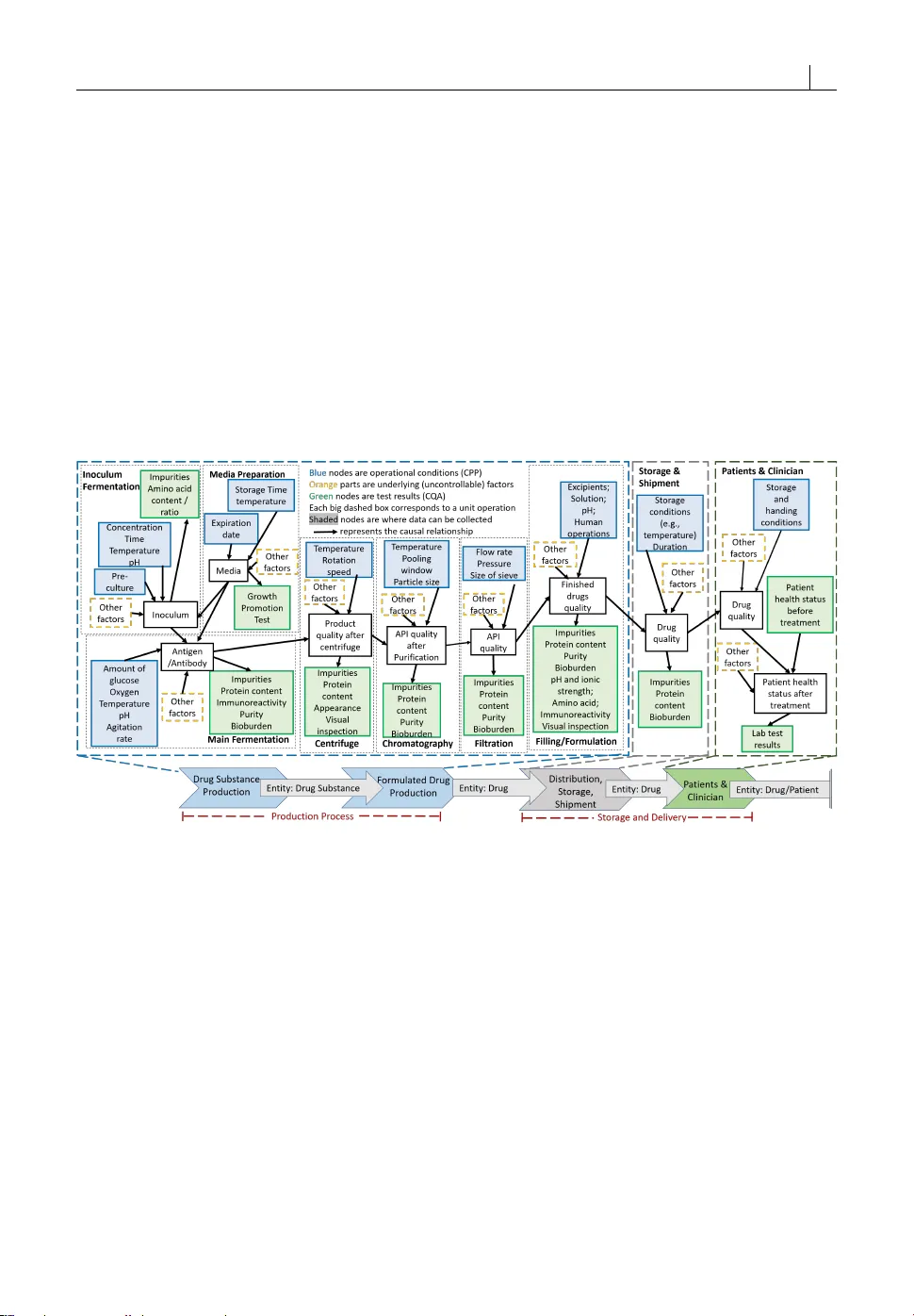
R E S E A R C H A R T I C L E In terpr etable Biomanufacturing Pr oc ess Risk and Sensitivity Analyses for Quality-b y-Design and S tability Con tr ol W ei Xie 1 | Bo W ang 1 | Cheng Li 2 | Dongming Xie 3 | Jar ed A uclair 4 1 Department of M echanical and Industrial Engineering, Northeastern U niversity , Boston, MA 02115, USA 2 Department of S tatistics and Applied Probability , N ational Univ ersity of Singapore, Singapor e 3 Department of Chemical E ngineering, University o f Massachusetts L o well, L owell, MA 01854, USA 4 Department of Chemistry and Chemical Biology , Northeastern U niversity , B oston, MA 02115, USA Correspondence W ei Xie, Departmen t of Mechanical and Industrial Engineering, N ortheastern University , Boston, MA 02115, USA Email: w.xie@northeastern.edu While biomanufacturing plays a signiﬁcant r ole in support- ing the economy and ensuring public health, it faces critical challenges, including complexity , high variability, lengthy lead time, and very limited process data, especially for per- sonalized new cell and gene biotherapeutics. Driven by these challenges, we propose an interpr etable seman tic bio- proc ess probabilistic knowledge graph and develop a game theory based risk and sensitivity analyses for production proc ess to facilitate quality-by-design and stability contr ol. Speciﬁcally , by exploring the causal relationships and inter- actions of critical process parameters and quality attributes (CPP s/C QAs ), w e creat e a Bayesian network based proba- bilistic knowledge graph characterizing the complex causal inter dependencies of all factors. Then, we intr oduce a Shap- ley value based sensitivity analy sis, which can correctly quan- tify the variation contribution from each input factor on the outputs (i.e., productivity , product quality). Since the bioproc ess model coeﬃcients are learned from limited pro- cess observations, we derive the Bayesian posterior distri- bution to quantify model uncertainty and further develop the Shapley value based sensitivity analysis to evaluate the impact of estimation uncertainty from each set of model co- 1 2 Bioproc ess Risk and Sensitivity Analyses eﬃcients. There for e, the proposed bioprocess risk and sen- sitivity analyses can identify the bottlenecks, guide the re- liable process speciﬁcations and the most informa tive data collection, and improv e production stability. K E Y W O R D S Bioproc ess risk analysis, sensitivity analysis, manufacturing process stability contr ol, Bayesian network, process causal interdependenc e 1 | I N T R O D U C T I O N Biomanufacturing is growing rapidly and playing an increasingly signiﬁcant role in supporting the economy and ensur- ing public health. F or example, the biopharmaceutical industry generated more than $300 billion in rev enue in 2019 and more than 40% of the drug products in the development pipeline were biopharmaceuticals (Rader and Langer, 2019). However , drug shortages have occurred at unprecedented rates over the past decade. The current systems are unable to rapidly produce new drugs to meet urgent needs in the presence of a major public health emergency. The CO VID-19 pandemic is having a prof ound impact globally and caused over 111 millions conﬁrmed cases by February , 2021. Even COVID-19 vaccines are discover ed, developing the production process and manufacturing the billions of doses needed to immunize the world’s population will be extr emely time-consuming using existing technologies, thus lengthening the time period of human and economic distress. It is critically important to speed up the bioproc ess development and ensure product quality consistency . Howe ver , biomanufacturing faces sever al critical challenges, including high complexity and variability , and lengthy lead time (Kaminsky and W ang, 2015). Biomanufacturing is based on living cells whose biological processes are very com- plex and have highly variable outputs. The productivity and product critical quality attributes (CQ As ) are determined by the interactions of hundreds of critical process parameters (CPPs ), including raw materials, media compositions, feeding strategy , and process operational conditions, such as pH and dissolved oxygen in the bioreactor . As new biotherapeutics (e.g., cell and gene therapies) become more and more “personalized" , the production, regulation pro- cedure, and analytical testing time required by biopharmaceuticals of complex molecular structure is lengthy , and the historical observations are relatively limited in particular for drugs in early stages of production process development. Theref or e, it is crucial to integr ate all sources of data and mechanism information, provide the risk- and science-based understanding of the complex bioprocess CPPs/CQAs causal interdependencies, and identify and control the key factors contributing the most to the output variation. This study can accelerate the development of productive and reliable biomanufacturing, facilitate building the quality into the production process or quality-by-design (Qb D ), support real- time monitoring and release, and reduce the time to market. V arious Process Analytical T echnologies (P A T) and methodologies have been proposed to improv e the bioprocess understanding and guide the process development, decision making, and risk control; see the review in Steinwandter et al. (2019). Most P A T s are based on multivariate data analysis; see Section 2. Or dinary or partial diﬀerential equations (ODEs/PDE s) based mechanistic models are developed for simulating individual biomanufacturing unit operations; see for example K yriak opoulos et al. (2018). On the other hand, various operations research/ managemen t (OR/OM) methods are also proposed for biomanufacturing system analytics and decision-making; see the review (Kaminsky and W ang, 2015). Overall, existing methodologies have the key limitations : (1) the multivariate statistics based P A T and Bioproc ess Risk and Sensitivity Analyses 3 OR/OM approaches focus on developing general methodologies without incorporating the bioprocess causal relation- ship and structural mechanism information, which limits their performance, interpretability , and adoption, especially with limited data; and (2) the mechanistic models are usually deterministic and focus on individual unit operations without providing an reliable integrated bioprocess learning and risk management framework. Driven by the critical challenges in the biomanufacturing industry , in this paper , we propose a bioprocess semantic probabilistic knowledge graph, characterizing the risk- and science-based understanding of integrated production process, which can integrate all sources of heterogeneous data and leverage the information from existing mechanism models and historical data. Then, we introduc e comprehensive and rigor ous bioprocess risk and sensitivity analyses, accounting for model risk, which can guide the process speciﬁcations and most informative data collection to facilitate the learning and improve the production reliability and stability (e.g., product quality consistency). The key contributions of this paper are three fold. First, by exploring the causal relationships and interactions of many factors within and between operation units (i.e., CPPs/C QAs ), such as raw materials, production process param- eters, and product quality , we consider a bioprocess ontology based data integration and develop a Bayesian network (BN) based bioprocess probabilistic knowledge graph, characterizing the process inherent stochastic uncertainty and causal interdependencies of all input and output factors. Second, building on the process knowledge graph, we in- troduce a game theory – Shapley value (SV) – based sensitivity analysis (SA), considering the complex bioprocess interdependencies, which can correctly quantify the contribution and criticality of each random input factor on the variance of outputs (i.e., productivity and product CQAs ), identify the bottlenecks, and accelerate the reliable biopro- cess speciﬁcations. Third, since the coeﬃcients of interpretable bioprocess model or probabilistic knowledge graph are estimated from limited real-world process data, which induces model uncertainty (MU) or model risk (MR), we further propose Bayesian uncertainty quantiﬁcation and Shapley value based model uncertainty sensitivity analysis to support process learning and faithfully assess the impact of estimation uncertainty from each set of model coeﬃ- cients. Thus, our study can: (1) identify the bottlenecks of bioprocess; (2) acceler ate the reliable process speciﬁcations and development to improv e the production process stability and facilitate QbD; and (3) support the most “informativ e" data collection to reduce the model risk of process probabilistic knowledge graph and improve the bioprocess understanding. This paper is organized as follows. In Section 2, we revie w the related literature on biomanufacturing process modeling and P A T s, Bayesian network, and process sensitivity analysis. In Section 3, we present the problem descrip- tion and summarize the proposed framework. In Section 4, we develop the Bayesian network (BN) based bioprocess probabilistic knowledge graph to characterize the risk- and science-based process understanding. W e derive the Shapley value (SV) based bioprocess sensitivity analysis in Section 5 to support the process speciﬁcations, improve the production stability, and ensure product quality consistency. We further introduc e the process model coeﬃcient uncertainty quantiﬁcation and Shapley value based sensitivity analysis studying the impact of each model coeﬃcient estimation uncertainty on process risk analysis and CPPs/C QAs criticality assessment in Section 6. We conduct the empirical study on the performance of our proposed framework in both simulation and real data analysis in Section 7, and then conclude with some discussion in Section 8. 2 | B A C K G R O U N D The Process Analytical T echnologies (P A T) are deﬁned as “a system for designing, analyzing and contr olling manufac- turing through timely measurements of critical quality and performance attributes of raw and in-process materials and processes, with the goal of ensuring ﬁnal product quality"; see Pharmaceutical Current Good Manufacturing Practices (C GMPs ) (2004). With the established process sensors and analyzers, such as near infrar ed spectroscopy , Raman 4 Bioproc ess Risk and Sensitivity Analyses spectrocop y , and multiwavelength ﬂuorescenc e, various multivariate data analysis approaches have been used for bioprocess P A T s, including principal component analysis (PCA) (Ayech et al., 2012), partial least squares (PLS) (De Lira et al., 2010), clustering (Prinsloo et al., 2008), multilinear regression (W echselber ger et al., 2012), artiﬁcial neural net- work (ANN) (Li and V enkatasubramanian, 2018), genetic algorithm (Sokolo v et al., 2018), elastic net (Severson et al., 2015), support vector machines (Li and Y uan, 2006), and root cause analysis (Borchert et al., 2019); see an overview in Rathore et al. (2010). Howev er , existing P A T approaches are usually based on generalized multivariate “black-bo x" approaches quantifying the input-output relationship without incorporating the bioprocess mechanism information. On the other hand, OR/OM methodology development for biomanufacturing analysis and decision making is still in its infancy (Kaminsky and Wang, 2015). Mixed integer linear programming (Lakhdar et al., 2007; Leachman et al., 2014), dynamic lot size model (Fleischhacker and Zhao, 2011), and queueing network and simulation models (Lim et al., 2004; Kulkarni, 2015) have been developed to study resour ce planning, scheduling and material consump- tion in biomanufacturing. Those approaches focus on developing general methodologies without fully exploring the bio-technology domain knowledge (e.g., causal relationship, structural information of the bioprocess ). Some recen t works, e.g., Martagan et al. (2016, 2017, 2018), account for physical-chemical characteristics and biology-induced randomness in either fermentation or chromato graphy stage, and develop Mark ov decision models to optimize the corresponding operational policies. F or complex systems, Bayesian network (BN) can be used to combine the expert knowledge with data and facil- itate data integration and process analysis in various applications. F or example, W ang et al. (2018) proposed a BN based knowledge management system for additive manufacturing. T roy anskaya et al. (2003) introduced a BN that combines evidence from gene co-expression and experimental data to predict whether two genes are functionally related. Moullec et al. (2013) provided a BN approach for system architectur e generation and evaluation, and T e- lenko and Seepersad (2014) applied probabilistic graphical model to study how the usage context factors, including human factors, situational factors, and product design factors, impact on the energy consumption of the lightweight vehicle to guide usage scenarios and vehicle designs. F urthermore, Bayesian posterior and belief propagation based risk assessment has been studied in information system security (F eng et al., 2014), water mains failure (Kabir et al., 2015), and supply chain (Ojha et al., 2018). Motiva ted by these studies, we propose a Bayesian network for modeling the complex interdependenc e of production process parameters and bio-drug properties, which can fully utilize the structural knowledge and causal relationship, and integrate the data from end-to-end bioprocess. Finally , we brieﬂy discuss the related literature on sensitivity analysis; see the review (Borg onovo and Plischke, 2016). The existing sensitivity analysis studies associated with Bayesian network tend to systematically vary one of network’ s parameter at a time while ﬁxing the other parameters and then obtain analytic expressions for the sensitiv- ity functions (V an der Gaag et al., 2007; Castillo et al., 1997). In our case, we are interested in stochastic uncertainty contributed by each factor , which is closely related to global probabilistic sensitivity analysis. Existing literatur e on global sensitivity analysis can be divided into several categories, including: (1) regression based methods, e.g., Helton (1993), which use the standardized regression coeﬃcients as sensitivity measure; (2) variance based methods (W ag- ner, 1995; Sobol, 1993) which assess the contribution of each random input based on expected reduction in model output variance; (3) functional ANOV A decomposition (Rabitz and Aliş, 1999) which provides variance decomposition under independence through high dimensional model representation theory; (4) density-based methods (Zhai et al., 2014) that directly quantify the output density without refer ence to a particular moment. Since the commonly used variance-based sensitivity measures (i.e., ﬁrst-order eﬀects and total eﬀects) fail to adequately account for probabilis- tic dependence of inputs and process structural interactions or interdependencies, Owen (2014) introduced a new sensitivity measure based on the game theory , called the Shapley V alue (SV). Song et al. (2016) further analyzed this measure and pr oposed a Monte Carlo algorithm for the estimation of Shapley values. Lundber g and L ee (2017) pro- Bioproc ess Risk and Sensitivity Analyses 5 posed Shapley value based uniﬁed framework for interpreting predictions. Inspired by these studies, building on the proposed BN-based bioprocess knowledge graph characterizing the process causal interdependencies, we introduc e SV -based probabilistic sensitivity analysis to assess the contribution or criticality of each random input (e.g., CPP and CQ A ) on the output variance, while accounting for the impact of model estimation uncertainty associated with each set of model coeﬃcients. 3 | P R O B L E M D E S C R I P T I O N A N D P R O P O S E D F R A M E W O R K W e create a probabilistic graph model characterizing the risk- and science-based understanding of causal interdependencies between bioprocess CPPs/C QAs, and then propose risk and sensitivity analyses for integrated biomanuf acturing process, accounting for model uncertainty . This study can: (1) provide a reliable guidance on process speciﬁcation, CPPs/CQ As monitoring, and most informative data collection; (2) facilitate production stability contr ol and quality-by-design (Qb D ); and (3) accelerate real-time release, speed up the time to market, and reduce the drug shortage. An illustration of biomanufacturing process is provided in Fig. 1 with a ﬁsh bone representa tion of bioprocess input factors introduced in each unit operation impacting on the outputs. The biomanufacturing process typically has sever al main unit operations, including: (1) media preparation, (2) inoculum fermenta tion, (3) main fermentation, (4) centrifugation( s ), (5) chromatography /puriﬁcation, (6) ﬁltration, (7) ﬁll and ﬁnish, and (8) quality control. Steps (1)–(3) belong to upstream cell culture, Steps (4)–(6) belong to downstream target protein puriﬁcation, and St eps (7)–(8) are for ﬁnished drug ﬁlling/formulation and ﬁnal product quality control testing. The inter actions of many factors impact the variability of outputs (e.g., drug quality, productivity). They can be divided into CPPs and CQAs in general; see the deﬁnitions of CPPs/C QAs in ICH Q8(R2) Guideline et al. (2009). CPP: At each process unit operation, CPPs are deﬁned as critical process parameters whose variability impacts on product CQAs, and therefor e should be monitored and controlled to ensure the process produces the desired quality . CQ A: A physical, chemical, biological, or microbiological property that should be within an appropriate limit, range, or distribution to ensure the desired product quality. Since the raw material attributes are outputs of release materials, they should be considered along with CPPs as impacting process variability . W e repr esent the syst em output (e.g., product CQAs, productivity) with a random variable, denoted by Y , which depends on CPPs/C QAs inputs, denoted by X , and other uncontrolled/ unc ontrollable input variables (e.g., contami- nation), modeled by residuals e . W e represen t the impact of complex interactions of input factors ( X , e ) throughout the production process on the response by Y = g ( X , e | θ θ θ ) , where the unknown function g ( X , e | θ θ θ ) , speciﬁed by model coeﬃcients θ θ θ , models the complex interactions of integrated bioprocess and characterizes the impact of random in- puts ( X , e ) on the output Y . For notation simpliﬁcation, we consider the unit-variate response/ output in the paper, and the proposed framework can be naturally extended to a vector of responses. T o provide the risk- and science-based production process understanding and guide the reliable process develop- ment, we need to correctly quantify all sources of uncertainties. There are two types of uncertainty: (1) bioprocess inherent stochastic uncertainty from CPPs/CQ As and other uncontrolled variables (i.e., randomness of X and e ), which can be reduced by the identiﬁcation of missed CPPs and tighter speciﬁcation of selected CPPs; and (2) model uncer- tainty (MU) (i.e., the estimation uncertainty of bioprocess model coeﬃcients θ θ θ ), which can be reduced by collecting 6 Bioproc ess Risk and Sensitivity Analyses F I G U R E 1 An illustration of general biomanufacturing process and ﬁsh-bone represen tation (W alsh, 2013). “most informativ e" process observations. Correctly quantifying all sources of uncertainty can facilitate learning, guide risk elimination/ contr ol, and improv e robust, automatic, and reliable bioprocess decision making. 3.1 | R evie w of Game Theory based Sensitivity Measur e - Shapley V alue In game theory , the Shapley value (SV) was originally introduced to evaluate the contribution of a player in a cooper- ative game Shapley (1953). A cooperative game is deﬁned as a set of players K = { 1 , 2 , . . . , K } , with a function c ( ·) that maps a subset of players to its corresponding payoﬀ , c : 2 K → Ò with c ( ∅ ) = 0 , where 2 K denotes the power set of K (i.e., the set of all subsets of K ). Thus, c ( J ) characterizes the total gain that the players in subset J ⊂ K can obtain by cooperation. The SV of player k ∈ K with respect to c ( · ) is deﬁned by Sh k = Õ J ⊂ K /{ k } ( K − | J | − 1 ) ! | J | ! K ! [ c ( J ∪ { k }) − c ( J ) ] , (1) where K = | K | is the total number of players and | J | is the size of subset J from K / { k } . This SV can be interpre ted as the average incremental payoﬀ by including player k over all possible cooperation group formations, i.e., J ⊂ K / { k } , and Sh k can be used to measure the contribution of the player k . This assessment approach satisﬁes the “eﬃciency property" that the sum of the SV s of all players equals the gain of the grand coalition, i.e., c ( K ) = Í K k =1 Sh k . The Shapley value was rec ently introduced for global sensitivity analysis to measure the variance of output con- tributed by each random input (Owen, 2014). Denote the set of inputs as U K = { U 1 , U 2 , . . . , U K } , and model the output V = η ( U K ) as a function η ( ·) of the inputs, accounting for their interactions. T wo most commonly used variance-based sensitivity measures are: (1) the ﬁrst-order eﬀect O k ≡ V ar ( V ) − E [ V ar ( V | U k ) ] that considers the variance reduction when we ﬁx U k ; and (2) the total eﬀect T k ≡ E [ V ar ( V | U − k ) ] that considers the expected remain- ing variance when all other factors, denoted by U − k , are ﬁxed. However , both measures fail to appropriately quantify Bioproc ess Risk and Sensitivity Analyses 7 the sensitivity or variance contribution when there exist probabilistic interdependenc e among inputs and process structural interaction (Song et al., 2016). Built on the SV from game theory, given a cooperativ e game with inputs U K as the players and the payo ﬀ as the incremental variance in output V induced by any index subset J ⊂ K , one can deﬁne the payoﬀ function as c ( J ) = V ar ( V ) − E [ V ar [ V | U U U J ] ] or c ( J ) = E [ V ar [ V | U U U − J ] ] . (2) Thus, Owen (2014) introduced a new SV-based sensitivity measure, with Sh U k , V computed by Equations (1) and (2). In this paper , we use c ( J ) = E [ V ar [ V | U U U − J ] ] in Equation (1), which can simplify the computation of the contribution from any random input U k on the output variance V ar ( V ) , Sh U k , V = Sh k . The SV-based sensitivity analysis over comes the limitations of ﬁrst-order eﬀect and total eﬀect measures by accounting for the interdependence of inputs and process interactions. The variance of output V can be decomposed into the contribution from each random input U k and we can deﬁne the criticality as the proportion of V ar ( V ) contributed from U k , denoted by p U k , V , V ar ( V ) = K Õ k =1 Sh U k , V and p U k , V = Sh U k , V V ar ( V ) . The main beneﬁts of SV over ﬁrst-order and total eﬀect sensitivity measures include: (1) the uncertainty contri- butions sum up to total variance of output; and (2) SV can automatically account for probabilistic dependence and structural interactions occurring in the complex production process. 3.2 | Summary of Proposed Interpr etable Bioprocess Model, Risk and Sensitivity Analyses for Integrated Bioprocess Stability Contr ol Fig. 2 pro vides the ﬂowchart of proposed risk and sensitivity analyses framework, which can accelera te learning of the end-to-end production process and guide the development of stable biomanufacturing. Parts I and II focus on modeling and reducing of process stochastic uncertainty . Part III focuses on analyzing and controlling the model risk. By exploring the causal rela tionships and interactions of CPPs/CQ As of raw materials/in-pr ocess materials/pr oduct within and between diﬀer ent process modules, in Section 4, we develop ontology based data integration and creat e an interpretable Ba yesian network (BN) based bioprocess semantic probabilistic knowledge graph, speciﬁed by the model coeﬃcients θ θ θ . This knowledge graph can characterize the risk- and science-based understanding of integrated bioprocess and quantify the causal interdependencies of inputs ( X , e ) and output Y . It is interpretable and extendable, which can support ﬂexible process modular design, incorporat e the existing mechanisms from diﬀerent modules and oper- ation units, quantify the bioproc ess causal interdependencies, and greatly reduce the dimensionality of bioprocess design space to guide the decision making. Building on this interpretable probabilistic knowledge graph, in Section 5, we develop the SV-based process risk and sensitivity analyses studying stochastic uncertainty , and derive variance decomposition to quantify the contribu- tion from each random input, V ar ( Y | θ θ θ ) = Õ X k Sh X k , Y ( θ θ θ ) + Õ e k Sh e k , Y ( θ θ θ ) , where Shapley values, Sh X k , Y ( θ θ θ ) and Sh e k , Y ( θ θ θ ) , measure the contributions from any CPP/ CQ A, X k ∈ X , and residual factor , e k ∈ e (repr esenting the impact of remaining uncontrolled factors on the CQA X k ), to the output variance 8 Bioproc ess Risk and Sensitivity Analyses F I G U R E 2 The ﬂowchart of proposed biomanufacturing process risk and sensitivity analyses framework. V ar ( Y | θ θ θ ) . F or any input factor W k (i.e., either X k or e k ), the criticality , p W k , Y ( θ θ θ ) ≡ Sh W k , Y ( θ θ θ ) / V ar ( Y | θ θ θ ) , can be used to identify the bottlenecks that contribute the most to V ar ( Y ) , and guide the process speciﬁcations to eﬃciently improve production process stability. The CPPs/CQAs X k with high criticality requires more restrict stability control, while the residual e k , with high impact on the output variance, can guide us to identify the ignored CPPs. Since the Shapley value (SV) based sensitivity analysis is developed based on game theory, its combination with bioprocess probabilistic knowledge graph, accounting for the complex causal inter dependencies, can corr ectly assess the risk eﬀect from each set of r andom input factors on the output variation. The “corr ect" proc ess model coeﬃcients, denoted by θ θ θ c , characterizing the bioprocess underlying probabilistic interdependenc e, is unknown and estimated by using the real-world process data, denoted by X . Given limited his- torical process data, the model risk or estimation uncertainty can have a large impact on the bioprocess risk and sensitivity analyses. Since the estimation uncertainty of model coeﬃcients at diﬀerent parts of bioprocess can be diﬀer ent and interdependent, the model uncertainty (MU) is quantiﬁed with the joint posterior distribution p ( θ θ θ | X ) . W e further develop the SV-based sensitivity analysis to study the impact of model uncertainty from each part of process in Section 6 , which can guide the “most informative " data collection to reduce the impact from model risk and eﬃciently impro ve the accuracy of bioprocess risk analysis and critiality assessment, especially for those factors contributing the most to the output variance. For any random input W k , the Shapley value Sh W k , Y is estimated with error , which can be contributed by the model coeﬃcients located along the paths propagating the uncertainty of W k to the output Y , denoted by θ θ θ ( W k , Y ) . W e introduce the BN-SV -MU sensitivity analysis to provide the compr ehensive study over the impact of model uncertainty , V ar ∗ [ Sh W k , Y | X ] = Õ θ ` ∈ θ θ θ ( W k , Y ) Sh ∗ θ ` h Sh W k , Y  e θ θ θ ( W k , Y )     X i = Õ θ ` ∈ θ θ θ ( W k , Y ) Sh ∗ θ `  Sh W k , Y   X  , (3) Bioproc ess Risk and Sensitivity Analyses 9 where the subscript “ ∗ " r epresents any measure calculated based on the posterior p ( θ θ θ | X ) and Sh ∗ θ ` [ · | X ] measures the contribution from coeﬃcient estimation uncertainty of θ ` ∈ θ θ θ ( W k , Y ) . In the proposed interpretable bioprocess model, θ ` can be interpreted as certain mechanistic coeﬃcients ( e.g., cell growth rate in the cell culture ). Thus, the decomposition in (3) provides the detailed information on how the model uncertainty of each part of integrated pro- duction process inﬂuences the estimation uncertainty of Sh W k , Y . T o illustrate the key ideas of the proposed bioprocess risk and sensitivity analyses, we use a simpliﬁed monoclonal antibody (mAbs) drug substance production example, including main fermentation, centrifuge, chromatograph, and ﬁltration; see the interactions in Fig. 3. W e consider the dominant CPPs/CQAs in each step, while the impacts of remaining factors are included in e . We are interested in the variance contribution (or criticality) from each CPP to drug substance protein content Y = X 20 , and also account for the impact of model uncertainty on criticality assessment. F I G U R E 3 An example illustration visualization of the integrated bioprocess sensitivity framework for criticality assessment and model uncertainty. The results of risk and sensitivity analyses can be visualized along the graph model for this bioprocess example; see Fig. 3. The process knowledge graph model is speciﬁed by coeﬃcients, θ θ θ = ( µ µ µ , v v v 2 , β β β ) , where µ µ µ and v v v 2 are the mean and variance vectors of all factors (listed in the table), and β β β quantiﬁes the eﬀects from parents’ nodes on each child node. The darkness of nodes indicates the criticality level of process factors, which can guide the better bioprocess speciﬁcation. The results show that X 4 contributes to 55 % variance of X 20 . In addition, the darkness of directed edges and circle boundaries indicates the distribution of model uncertainty in the process. For instance, the variance of dissolved oxygen in bioreactor , v 2 4 , has dominant model uncertainty impact on the estimation uncertainty of criticality p X 4 , Y , which suggests additional data should be collected to improve the estimation of v 2 4 . W e will revisit this example and use it to study the performance of proposed framework in Section 7.1. 4 | I N T E R P R E TA B L E B I O P R O C E S S P R O B A B I L I S T I C M O D E L D E V E L O P M E N T W e dev elop an interpretable bioprocess probabilistic model, which can be extendable to end-to-end biomanfactur- ing supply chain and support evidence-based biopharmaceutical production process development. The model can incorporate the existing mechanism models from each module and unit operation, and facilitate the learning from distributed and heterogeneous process data. In this section, we develop a Bayesian network (BN) based interpretable 10 Bioproc ess Risk and Sensitivity Analyses bioprocess probabistic knowledge graph, which can characterize the complex CPPs/CQ As causal interdependencies and support ﬂexible modular biomanfuacturing development. By exploring the causal relationships and interactions, we consider bioprocess ontology-based data integration , which can connect all distributed and heterogeneous data collected from bioprocess; see more description in Online Appendix A. This relational graph can enable the connectivity of end-to-end process. Nodes represen t factors (i.e., CPPs/C QAs, media feed, bioreactor operating conditions, other uncontrolled factors) impacting the process outputs, and the directed edges model the causal relationships. Within each module, which can be each phase of cell cul- ture process (such as cell growth and production phases) or each unit operation, we can model complex interactions, e.g., biological/ph ysical/ chemical interactions. In the relational graph, the shaded nodes repr esent the variables with real-world observations, including the testing and sensor monitoring data of CPPs/CQ As for raw materials, opera- tion conditions, and intermediate/ﬁnal drug products. The unshaded nodes repr esent variables without observations and residuals, including quality status of intermediate and ﬁnal drug products, and other uncontrollable factors ( e.g., contamination ) introduced during the process unit operations. Since bio-products have very complex structures, we cannot observe the underlying complete quality status and the monitoring of CQAs can carry partial information. Build- ing on the bioprocess relational graph, we develop a BN based probabilistic graphical model composing of random CPPs/C QAs/ r esiduals factors and their conditional dependencies via directed edges. It can characteriz e the probabilis- tic causal interdependencies among all factor s of integr ated bioprocess. T o make it easy to follow , we ﬁrst pro vide a simple illustration example of cell culture process, including two phases, to present the key ideas of modular bioprocess modeling , and then develop the complete probabilistic knowledge graph model for general integrated bioprocess. Speciﬁcally , we use a simple bioreactor fermentation example with two phases (i.e., cell growth and production phases; see Fig. 4) to illustrate the probabilistic graphical model development. It is based on the causal relationships and interactions between CPPs and CQ As. Each node repr esents a CPP /C QA with a random variable X modeling its variability . Each directed edge represents the causal impact of parent node X i on child node X j . The pattern-ﬁll nodes ( X 1 , X 2 , X 3 ) repr esent the CPPs. The solid ﬁll nodes ( X 6 , X 7 ) repr esent the monitored CQAs of intermediate materials and drug products. The nodes X 4 and X 5 repr esent the underlying status of working cells after cell growth phase and the protein/impurity structure after cell production phase. The CQAs X 6 and X 7 repr esent the partial information of quality variables X 4 and X 5 . Ex cept the CPPs X 1 , X 2 , X 3 , the impacts from other uncontrolled factors introduced during two phases of cell culture are modeled through e 0 4 and e 0 5 . F I G U R E 4 L eft: knowledge relational graph; Right: simpliﬁed knowledge graph. Since it is hard to uniquely specify the underlying cells/ pro teins with very complex structures, X 4 and X 5 are Bioproc ess Risk and Sensitivity Analyses 11 hidden, which can lead to an identiﬁcation issue. T ypically, the non-identiﬁable BN with hidden nodes is transformed to the equivalent BN by structural simpliﬁcation to avoid analytical issues (see Chapter 19 in Koller and F riedman (2009)). Thus, we simplify and transform the relational graphical model to a graph without hidden nodes, depicted in the right panel of Fig. 4. The new residual e 6 in updated graph accounts for both original residual e 0 4 and also the uncertainty of underlying cell health status, X 4 , impacting on CQA X 6 , similar for new residual e 7 . Accor ding to the right plot in Fig. 4, the sources of bioproc ess stochastic uncertainty impacting on the variability of X 7 include CPPs, ( X 1 , X 2 , X 3 ) , and other factors with the impact repr esented by residuals ( e 6 , e 7 ) . Thus, we have CPPs X 1 , X 2 as inputs and CQA X 6 as output for the ﬁrst cell gro wth phase, and have CQA X 6 and CPP X 3 as inputs and X 7 as output for the second protein production phase. T o study the impact of each CPP on the CQA of interest (i.e., X 6 and X 7 ), we can decompose the variance of X 6 and X 7 into the contributions from X 1 , X 2 and X 3 , and remaining parts coming from e 6 and e 7 ; see the process risk and sensitivity analyses in Section 5. In this way , we can identify the main sources of uncertainty and quantify their impacts, which can guide the CPPs/C QAs speciﬁcations and the quality contr ol to impro ve the product quality stability. Now we describe the BN-based bioprocess model for general situations. Suppose that the integrated bioprocess can be repr esented by a probabilistic graphical model with m + 1 nodes: m proc ess factors (deno ted by X ) and a single response, denoted by Y , such as the impurity concen tration or pro tein content. Let the ﬁrst m p nodes representing CPPs X p = { X 1 , X 2 , . . . , X m p } , the next m a nodes represen ting CQAs X a = { X m p +1 , X m p +2 , . . . , X m } , and the last node repr esenting the response Y , X m +1 with m = m p + m a . The modular bioprocess probabilistic knowledge graph can be modeled by marginal and conditional distributions of each node as follows: X k ∼ N ( µ k , v 2 k ) for CPP X k with k = 1 , 2 , . . . , m p , (4) X k = f ( P a ( X k ) ; θ θ θ k ) + e k for CQA X k with k = m p + 1 , . . . , m + 1 (5) where N ( u , v 2 ) denotes the normal distribution with mean u and variance v 2 , and P a ( X k ) denotes the parent nodes of X k . By applying central limit theory (CL T), we assume that the residual e k ∼ N ( 0 , v 2 k ) with the conditional variance v 2 k ≡ V ar [ X k | P a ( X k ) ] . Since the amount of real-world bioprocess batch data is often very limited, Gaussian distribution is used to model the variability of each variable or node, which is often used in the existing biopharmaceutical studies (see for example Coleman and Block (2006)). It also makes the process risk and sensitivity analyses tractable. The proposed probabilistic knowledge graph is a hybrid model of integrated bioprocess, which can leverag e the existing mechanisms and learn from real-world process data. Basically, the prior of the function f ( · ) in a generaliz ed regr ession model (5) can be speciﬁed based on the existing knowledge on underlying bioprocess mechanisms (e.g., biophysic- ochemical kinetics) within each module of bioprocess; see for example K yriak opoulos et al. (2018); Lu et al. (2018); Doran (1995). The unknown model coeﬃcients θ θ θ k (e.g., cell growth rate, media consumption rate ) need be estimated from process data. In this paper, we consider linear function accounting for the main eﬀects, i.e., X k = µ k + Õ X j ∈ P a ( X k ) β j k ( X j − µ j ) + e k for CQA X k with k = m p + 1 , . . . , m + 1 (6) where the coeﬃcient β j k can be used to measure the eﬀect from the parent node X j to child node X k . Her e, we use some illustrative examples to brieﬂy show how the proposed Bayesian network based process probabilistic model allows us to incorporate the existing bioprocess mechanisms. We ﬁrst consider the cell exponential growth mechanism for the fermentation step, x = x 0 e µ t , where x 0 and x denote the starting and ending cell densities, and µ is the unknown growth rate. This is a commonly used mechanism model in biomanufacturing industry; see more 12 Bioproc ess Risk and Sensitivity Analyses information in Doran (2013). Suppose that there is a ﬁxed cell culture duration t . By doing the log transformation and setting X k = log ( x 0 ) , X k +1 = log ( x ) and β 0 = µ t , we can take the exponential growth mechanism as prior and get the hybrid probabilistic model for the exponential growth phase in fermentation or cell culture process, X k +1 = β 0 + X k + e k , where e k repr esents the residual term characterizing the integrated eﬀect from many other factors and it follow s a Gaussian distribution by following CL T . Notice that it is a special case of BN-based process model (6). The similar idea can be applied to the situations where we have PDE/ODE-based bioprocess kinetics mechanism models, d d t x ( t ) = f ( x ( t ) ; θ t ) ≈ x ( t k +1 ) − x ( t k ) t k +1 − t k = f ( x ( t k ) ; θ t k ) , where x ( t ) can represent the concentr ations of protein and metabolite waste at time t and θ t can denote the nonsta- tionary growth rate. W e can take the existing mechanism model as the prior knowledge of production process. By applying the ﬁnite diﬀerence on the gradient d x ( t ) / d t and ﬁrst-order T aylor appro ximation on function f ( ·) , we can construct a probabilistic hybrid model matching with the formula in Equation (6), which can leverage the information from existing PDE/ODE-based bioprocess kinetics mechanism models. This approximation can be very accurate if the data are collected from real-time production process sensor monitoring with high sampling frequency . The complex bioprocess CPPs/CQ As causal interdependencies are characterized by the BN-based probabilistic knowledge graph. Given the model parameters θ θ θ = ( µ µ µ , v v v 2 , β β β ) with mean µ µ µ = ( µ 1 , . . . , µ m +1 ) > , conditional variance v v v 2 = ( v 2 1 , . . . , v 2 m +1 ) > , and linear coeﬃcients β β β = { β j k ; k = m p + 1 , . . . , m + 1 and X j ∈ P a ( X k ) } , the conditional distribution for each CQA node X k becomes, p ( X k | P a ( X k ) ) = N ©  « µ k + Õ X j ∈ P a ( X k ) β j k ( X j − µ j ) , v 2 k ª ® ¬ for k = m p + 1 . . . , m + 1 . F or any CPP node X k without parent nodes, P a ( X k ) is an empty set and P ( X k | P a ( X k ) ) is just the marginal distribu- tion P ( X k ) in (4). Theref ore, the joint distribution characterizing the inter dependencies of CPPs and CQAs involv ed in the production process can be written as p ( X 1 , X 2 , . . . , X m +1 ) = Î m +1 k =1 p ( X k | P a ( X k ) ) . 5 | P R O C E S S R I S K A N D S E N S I T I V I T Y A N A LY S E S Given the bioprocess probabilistic knowledge graph speciﬁed by the coeﬃcients θ θ θ = ( µ µ µ , v v v 2 , β β β ) , we develop the BN-SV based sensitivity analysis for integr at ed production pr ocess and quantify the criticality of each r andom input f actor measuring its contribution to the output variance V ar ( X m +1 ) . This study can guide the CPPs/CQAs speciﬁcation and improve the production process stability. T o make it easy to follow , we start with a simple illustration example, provide the general process risk and sensitivity analyses, and then present the algorithm at the end of this section. W e again use the simple example in Fig. 4 to illustrate the results of proposed BN-SV based bioprocess risk and sensitivity analyses, which can decompose the output variance of protein/impurity concentration X 7 after fermenta- tion process to each random input – including X 1 , X 2 , X 3 , e 6 , e 7 – as V a r ( X 7 | θ θ θ ) = ( β 16 β 67 ) 2 v 2 1 | {z } contribution from X 1 + ( β 26 β 67 ) 2 v 2 2 | {z } contribution from X 2 + β 2 37 v 2 3 | {z } contribution from X 3 + β 2 67 v 2 6 | {z } contribution from e 6 + v 2 7 | {z } contribution from e 7 . (7) The variance contribution from each random input, denoted by W k (i.e., X 1 , X 2 , X 3 , e 6 , e 7 ), depends on its variance v 2 k Bioproc ess Risk and Sensitivity Analyses 13 and the product of coeﬃcients β β β located along the paths propagating the uncertainty from W k to the output X 7 ; see Fig. 5. The darker blue ﬁlled node (i.e., cell growth phase CPP X 2 , feed rate) contributes more to the output variance and has higher criticality. Thus, to eﬃciently reduce the output variance, it requires more restrictive stability control. The high impact of e 7 (with darker color) can guide us to identify unrecogniz ed or missed CPPs. F I G U R E 5 A simple example to illustrate BN-SV based process risk and sensitivity analysis. This simple example illustrates that the proposed production process BN-SV risk and sensitivity analyses and the CPPs/CQAs criticality assessment are based on the bioprocess probabilistic knowledge graph, characterizing the complex CPPs/CQ As causal interdependencies and accounting for all sources of process inherent uncertainty, which can (1) guide the process speciﬁcations; (2) impro ve the product quality consistency and bioproc ess stability; and (3) advance the risk- and science-based understanding on bioprocess. Now we presen t the general process risk and sensitivity analyses. We ﬁrst derive the Shapley value (SV) quanti- fying the contribution of each random input factor from CPPs X p and other factors e to V ar ( X m +1 ) , which accounts for cases with dependent input factors. Acc ording to the Gaussian BN model presented in (4) and (6), we can write X m +1 = µ m +1 + m p Õ k =1 γ k , m +1 ( X k − µ k ) + m +1 Õ k = m p +1 γ k , m +1 e k , (8) where the weight coeﬃcient of any CPP X k to CQA X n with k ≤ m p < n ≤ m + 1 , γ k n = β k n + Õ m p < ` < n β k ` β ` n + Õ m p < ` 1 < ` 2 < n β k ` 1 β ` 1 ` 2 β ` 2 n + . . . + β k , m p +1 β m p +1 , m p +2 . . . β n − 1 , n , (9) the weight coeﬃcient of any e k to a CQA node X n with m p < k < n ≤ m + 1 , γ k n = β k n + Õ k < ` < n β k ` β ` n + Õ k < ` 1 < ` 2 < n β k ` 1 β ` 1 ` 2 β ` 2 n + . . . + β k , k +1 β k +1 , k +2 . . . β n − 1 , n ; (10) and γ n n = 1 for any n ; see the derivation for (8) in Appendix B. The weight coeﬃcient γ k n is the product sum of β β β located along the paths from node X k to node X n in the graph model. L et W W W = { X 1 , . . . , X m p , e m p +1 , . . . , e m +1 } , { W 1 , W 2 , . . . , W m +1 } represen t all random input factors, with the index set K = { 1 , 2 , . . . , m + 1 } . Then, the SV for the k -th factor W k is, Sh W k , X m +1 = Õ J ⊂ K /{ k } ( m − | J | ) ! | J | ! ( m + 1 ) ! [ c ( J ∪ { k }) − c ( J ) ] . 14 Bioproc ess Risk and Sensitivity Analyses Based on (8), we compute the cost function, c ( J ) = E [ V ar [ X i | W W W − J ] ] = Õ k ∈J γ 2 k , m +1 V ar ( W k ) + 2 Õ k 1 < k 2 ∈ J γ k 1 , m +1 γ k 2 , m +1 Cov ( W k 1 , W k 2 ) . The random input factors, W W W = ( X 1 , . . . , X m p , e m p +1 , . . . , e m +1 ) , including CPPs and residual terms introduced at each CQ A nodes, are often independent as the real biomanufacturing process speciﬁcation is often based on each CPP or CQ A. T o make the proposed framework general, we consider the potential interdependence between some inputs W k 1 and W k 2 with k 1 , k 2 , and the covariance Cov ( W k 1 , W k 2 ) can be estimated by using the process data. Then, for each W k and J ⊂ K / { k } , we can obtain c ( J ∪ { k }) − c ( J ) = γ 2 k , m +1 V ar ( W k ) + 2 Õ ` ∈ J γ k , m +1 γ ` , m +1 Cov ( W k , W ` ) . Given the BN-based bioprocess knowledge graph model parameters θ θ θ , by applying (1), we can derive the Shapley value, Sh W k , X m +1 ( θ θ θ ) , characterizing the contribution from any input factor W k to the output variance, Sh W k , X m +1 ( θ θ θ ) = γ 2 k , m +1 V ar ( W k ) + Õ ` , k γ k , m +1 γ ` , m +1 Cov ( W k , W ` ) . (11) The derivation of (11) is provided in Appendix C. Therefor e, we can decompose the variance of output X m +1 and estimate the contribution from each random input from X p and e , V ar ( X m +1 | θ θ θ ) = Õ Sh W k , X m +1 ( θ θ θ ) = m p Õ k =1 Sh X k , X m +1 ( θ θ θ ) + m +1 Õ k = m p +1 Sh e k , X m +1 ( θ θ θ ) . (12) Equation (12) can be used to identify the dominant factors in X p and e contributing the most to the output variance, which can guide the CPPs identiﬁcation and process speciﬁcation to improve the process stability and quality consis- tency . As a result, the criticality of any input factor W k can be calculated as p W k , X m +1 ( θ θ θ ) ≡ Sh W k , X m +1 ( θ θ θ ) / V ar ( X m +1 | θ θ θ ) . Notic e that for any independent input factor W k , the SV in Equation (11) is reduced to Sh W k , X m +1 ( θ θ θ ) = γ 2 k , m +1 v 2 k . Under the case that all input factors W W W are mutually independent, the variance decomposition Equation (12) can be written as V ar ( X m +1 | θ θ θ ) = Í γ 2 k , m +1 v 2 k , which gives the example results in Equation (7). This risk and sensitivity analyses can be applied to any part of production process including one or multiple modules. Under this situation, the input factors W W W include those nodes without parent node within the considered range of production (i.e., CPPs, CQ As or uncontr olled factors), and output of interest X i is certain CQA at the end of the procedur e. F or example, in Fig. 5, we consider the subgraph, including { X 3 , X 6 , X 7 } , for cell production phase with the starting CQA X 6 carrying the information from previous cell growth phase. W e can study the impacts of X 6 and CPP X 3 on the variability of CQA X 7 . The SV of any input W k and the variance decomposition of X i , still follow Equations (11) and (12) by replacing the output X m +1 with X i . The criticality of W k on X i can be measured by proportion p W k , X i ( θ θ θ ) = Sh W k , X i ( θ θ θ ) / V ar ( X i | θ θ θ ) . Given the BN parameters θ θ θ , we summarize the proc edure for production process BN-SV based sensitivity anal- ysis in Algorithm 1, in which we consider several consecutive operation steps, and our objective is to quantify the contribution of each random factor in W W W to V ar ( X i | θ θ θ ) . Bioproc ess Risk and Sensitivity Analyses 15 Algorithm 1: Proc edure for Production Process BN-SV based Sensitivity Analysis Input: BN parameters θ θ θ , group of input factors W W W , response node X m +1 . Output: V arianc e decomposition of X i in terms of all random inputs within W W W . (1) Calculate the Shapley value Sh W k , X m +1 ( θ θ θ ) by using Equation (11), which measures the contribution from W k to the variance of response CQA X m +1 ; (2) Pro vide the variance decomposition of V ar ( X m +1 | θ θ θ ) by using Equation (12), and obtain the criticality of W k on the variance of X m +1 : p W k , X m +1 ( θ θ θ ) = Sh W k , X m +1 ( θ θ θ ) / V ar ( X m +1 | θ θ θ ) . 6 | S E N S I T I V I T Y A N A LY S I S F O R M O D E L R I S K R E D U C T I O N Since the underlying true process model coeﬃcients θ θ θ c are unknown, given ﬁnite real-world data X , there exists the model uncertainty (MU) characterizing our limited knowledge on the probabilistic interdependence of integrated bio- process. T o study the impact of MU on the production process risk and sensitivity analyses for stochastic uncertainty and further assess CPPs/CQAs criticality , we propose the BN-SV -MU based uncertainty quantiﬁcation and sensitivity analysis , which can guide the proc ess monitoring and “most informativ e" data collection. In Section 6.1, we dev elop the posterior p ( θ θ θ | X ) and a Gibbs sampler to generate posterior samples, e θ θ θ ( b ) ∼ p ( θ θ θ | X ) with b = 1 , 2 , . . . , B , quantify- ing the model uncertainty , and then we quantify the overall impact of model uncertainty on the process risk analysis and CPPs/C QAs criticality assessment. In Section 6.2, we propose the BN-SV -MU based sensitivity analysis, which can study the impact of each model coeﬃcient(s) estimation uncertainty on the process risk analysis and criticality assessment; see the result visualization in Fig. 3. 6.1 | Bay esian Learning and Model Unc ertainty Quantiﬁcation W e consider the case with R batches of complete production process data, denoted as X = { ( x ( r ) 1 , x ( r ) 2 , . . . , x ( r ) m +1 ) , r = 1 , 2 , . . . , R } . Without strong prior information, we consider the following conjugate (vague ) prior (with initial hyperpa- rameters giving relatively ﬂat density), p ( µ µ µ , v v v 2 , β β β ) = m +1 Ö i =1 p ( µ i ) p ( v 2 i ) · Ö i , j p ( β i j ) , (13) with p ( µ i ) = N ( µ ( 0 ) i , σ ( 0 ) 2 i ) , p ( v 2 i ) = Inv- Γ κ ( 0 ) i 2 , λ ( 0 ) i 2 ! and p ( β i j ) = N ( θ ( 0 ) i j , τ ( 0 ) 2 i j ) , where Inv- Γ denotes the inverse- gamma distribution. Given the data X , by applying the Bayes’ rule, we can obtain the posterior distribution p ( µ µ µ , v v v 2 , β β β | X ) ∝ R Ö r =1 " m +1 Ö i =1 p ( x ( r ) i | x ( r ) P a ( X i ) ) # p ( µ µ µ , v v v 2 , β β β ) , (14) quantifying the model uncertainty. Then, we develop a Gibbs sampler to generate the posterior samples from (14) quantifying the model uncertainty . W e derive the conditional posterior for each parameter in ( µ µ µ , v v v 2 , β β β ) . Let µ µ µ − i , v v v 2 − i and β β β − i j denote the collection of parameters µ µ µ , v v v 2 , β β β excluding the i -th or ( i , j ) -th element. L et S ( X i ) denote the set of direct succeeding or child 16 Bioproc ess Risk and Sensitivity Analyses nodes of node X i . W e ﬁrst derive the conditional posterior for the coeﬃcient β i j , p ( β i j | X , µ µ µ , v v v 2 , β β β − i j ) = N ( θ ( R ) i j , τ ( R ) 2 i j ) , (15) where θ ( R ) i j = τ ( 0 ) 2 i j Í R r =1 α ( r ) i m ( r ) i j + v 2 j θ ( 0 ) i j τ ( 0 ) 2 i j Í R r =1 α ( r ) 2 i + v 2 j and τ ( R ) 2 i j = τ ( 0 ) 2 i j v 2 j τ ( 0 ) 2 i j Í R r =1 α ( r ) 2 i + v 2 j with α ( r ) i = x ( r ) i − µ i and m ( r ) i j = ( x ( r ) j − µ j ) − Í X k ∈ P a ( X j ) / { X i } β k j ( x ( r ) k − µ k ) . Then, we derive the conditional posterior for v 2 i = V ar [ X i | P a ( X i ) ] with i = 1 , 2 , . . . , m + 1 , p ( v 2 i | X , µ µ µ , v v v 2 − i , β β β ) = Inv- Γ κ ( R ) i 2 , λ ( R ) i 2 ! , (16) where κ ( R ) i = κ ( 0 ) i + R , λ ( R ) i = λ ( 0 ) i + Í R r =1 u ( r ) 2 i and u ( r ) i = ( x ( r ) i − µ i ) − Í X k ∈ P a ( X i ) β k i ( x ( r ) k − µ k ) . After that, we derive the conditional posterior for the mean parameter µ i with i = 1 , 2 , . . . , m + 1 for any CPP/C Q A, p ( µ i | X , µ µ µ − i , v v v 2 , β β β ) ∝ p ( µ i ) R Ö r =1       p ( x ( r ) i | x ( r ) P a ( X i ) ) Ö j ∈S ( X i ) p ( x ( r ) j | x ( r ) P a ( X j ) )       = N ( µ ( R ) i , σ ( R ) 2 i ) , (17) where µ ( R ) i = σ ( R ) 2 i       µ ( 0 ) i σ ( 0 ) 2 i + Í R r =1 a ( r ) i v 2 i + Í R r =1 Í X j ∈ S ( X i ) β i j c ( r ) i j v 2 j       and 1 σ ( R ) 2 i = 1 σ ( 0 ) 2 i + R v 2 i + Í X j ∈ S ( X i ) R β 2 i j v 2 j with a ( r ) i = x ( r ) i − Í X k ∈ P a ( X i ) β k j ( x ( r ) k − µ k ) and c ( r ) i j = β i j x ( r ) i − ( x ( r ) j − µ j ) + Í X k ∈ P a ( X j ) / { X i } β k j ( x ( r ) k − µ k ) . The Gibbs sampler iteratively draws the posterior samples of ( µ µ µ , v v v 2 , β β β ) by applying the conditional posterior distributions given in (15), (16), and (17) until converg ence (Gelman et al., 2004). Besides the case with complete production data, we often have additional incomplete batch data. Since the lead time for biopharmaceutical production is lengthy (Otto et al., 2014), we can have some batches in the middle of production. In addition, the bio-drug quality requirements are restricted, especially for human drugs. F ollowing the quality control, we could discard some batches after main fermentation or even in the middle of downstream puriﬁcation. Thus, we provide the Gibbs sampler (see Algorithm 3) for both cases with complete or mixing data in Appendix D.2. Next, we study the impact model uncertainty on the bioprocess risk and sensitivity analyses and CPPs/CQ As criticality assessment. Based on Section 5, the contribution from any random input factor W k to the output variance V ar ( X m +1 ) is measured by the Shapley value, Sh W k , X m +1 ( θ θ θ c ) . The unknown parameters θ θ θ c specifying the underlying process probabilistic model are estimated by using limited real-world data X . Thus, the estima- tion uncertainty of the contribution from factor W k can be quantiﬁed by the posterior distribution, Sh W k , X m +1 ( e θ θ θ ) with e θ θ θ ∼ p ( θ θ θ | X ) . W e can use the posterior mean to estimate the expected variance contribution and crit- icality , E ∗ [ Sh W k , X m +1 | X ] ≡ E ∗ p ( θ θ θ | X ) [ Sh W k , X m +1 ( e θ θ θ ) | X ] and E ∗ [ p W k , X m +1 | X ] ≡ E ∗ p ( θ θ θ | X ) [ p W k , X m +1 ( e θ θ θ ) | X ] , where p W k , X m +1 ( e θ θ θ ) = Sh W k , X m +1 ( e θ θ θ ) / V ar ( X m +1 | e θ θ θ ) . The posterior variance is used to quantify the overall estimation un- certainty induced by model uncertainty, V ar ∗ [ Sh W k , X m +1 | X ] ≡ V ar ∗ p ( θ θ θ | X ) [ Sh W k , X m +1 ( e θ θ θ ) | X ] and V ar ∗ [ p W k , X m +1 | X ] ≡ V ar ∗ p ( θ θ θ | X ) [ p W k , X m +1 ( e θ θ θ ) | X ] . Since we do not have the closed form solutions, we can estimate the posterior mean and variance of Sh ( W k ) and p W k , X m +1 through the sampling approach. By applying the Gibbs sampler in Appendix D, we can generate posterior samples e θ θ θ ( b ) ∼ p ( θ θ θ | X ) with b = 1 , 2 , . . . , B . At any e θ θ θ ( b ) , we can compute Sh W k , X m +1 ( e θ θ θ ( b ) ) following the descrip- Bioproc ess Risk and Sensitivity Analyses 17 tion in Section 5. The expected contribution from W k to the variance of X m +1 is estimated by b E ∗ [ Sh W k , X m +1 | X ] = ¯ Sh W k , X m +1 ( X ) = 1 B Í B b =1 Sh W k , X m +1 ( e θ θ θ ( b ) ) . And the overall estimation uncertainty can be estimated by sample vari- ance, d V ar ∗ [ Sh W k , X m +1 | X ] = 1 B − 1 B Õ b =1 h Sh W k , X m +1 ( e θ θ θ ( b ) ) − ¯ Sh W k , X m +1 ( X ) i 2 . (18) Similarly , we can estimate the expected criticality by b E ∗ [ p W k , X m +1 | X ] = ¯ p W k , X m +1 = 1 B Í B b =1 p W k , X m +1 ( e θ θ θ ( b ) ) and estimate the overall estimation uncertainty by d V ar ∗ [ p W k , X m +1 | X ] = 1 B − 1 B Õ b =1 h p W k , X m +1 ( e θ θ θ ( b ) ) − ¯ p W k , X m +1 i 2 . (19) 6.2 | Sensitivity Study for Model Unc ertainty Since there is often limited process data in biomanufacturing, model uncertainty tends to be large. W e propose the BN-SV -MU based sensitivity analysis studying the eﬀect of estimation uncertainty of each model coeﬃcient, which can guide the process monitoring and “most informativ e" data collection. W e provide the CPPs/CQ As criticality estimation uncertainty quantiﬁcation and BN-SV -MU based sensitivity analysis in Algorithm 2. Speciﬁcally, Steps (1)– (3) evaluate V ar ∗ [ Sh W k , X m +1 | X ] quantifying the over all estimation uncertainty of Sh W k , X m +1 . Steps (4)–(13) further study the impact from each model coeﬃcient estimation uncertainty . Her e we use V ar ∗ [ Sh W k , X m +1 | X ] for illustration and the similar procedur e can be applied to CPPs/CQ As critical- ity assessment V ar ∗ [ p W k , X m +1 | X ] . L et θ θ θ ( W k , X m +1 ) ⊂ θ θ θ represent the subset of model coeﬃcients that impacts on Sh ( W k | θ θ θ ) estimation. Notice that µ µ µ has no impact on Sh W k , X m +1 ( θ θ θ ) . Since SV can account for the probabilistic de- pendence of model coeﬃcient estimation uncertainty, characterized by the joint posterior distribution p ( θ θ θ | X ) , and bioprocess structural interactions, we can measure the contribution from any parameter θ ` ∈ θ θ θ ( W k , X m +1 ) through the posterior variance decomposition, V ar ∗ [ Sh W k , X m +1 | X ] = Õ θ ` ∈ θ θ θ ( W k , X m +1 ) Sh ∗ θ ` h Sh W k , X m +1  e θ θ θ     X i = Õ θ ` ∈ θ θ θ ( W k , X m +1 ) Sh ∗ θ `  Sh W k , X m +1   X  . The proposed BN-SV-MU sensitivity analysis can provide the comprehensive and interpretable understanding on how model uncertainty impacts on the process risk analysis and identify those parameters θ ` contributing the most on the estimation uncertainty of Sh W k , X m +1 ( θ θ θ ) . Then, we derive SV measuring the estimation uncertainty contribution from each θ ` , Sh ∗ θ `  Sh W k , X m +1   X  = Õ J ⊂ L k /{ ` } ( L k − | J | − 1 ) ! | J | ! L k ! [ c ( J ∪ { ` }) − c ( J ) ] . Denote the size of relevan t parameters by L k = | θ θ θ ( W k , X m +1 ) | and denote the index set by L k , θ θ θ ( W k , X m +1 ) = θ θ θ L k . We further denote any subset by θ θ θ J ⊂ θ θ θ ( W k , X m +1 ) with size J = | θ θ θ J | and the corresponding index set J = { J ( 1 ) , J ( 2 ) , . . . , J ( J ) } ⊂ L k . F or any J ⊂ L k , the cost function is given as, c ( J ) = E ∗ p ( θ θ θ L k −J |X ) [ V ar ∗ p ( θ θ θ J | θ θ θ L k −J , X ) [ Sh W k , X m +1 | e θ θ θ L k − J ] ] , (20) 18 Bioproc ess Risk and Sensitivity Analyses Algorithm 2: Proc edure for the BN-SV-MU Based UQ and SA Input: BN structure G ( N | θ θ θ ) , data X , number of samples N π , B , B O and B I , index subset L k . Output: Return c c Sh ∗ θ `  Sh W k , X m +1   X  and c Sh ∗ θ `  p W k , X m +1   X  for any W k ∈ W W W = { X p ∪ X a ∪ e } . (1) Call Algorithm 3 in Appendix D.3 to obtain the posterior samples e θ θ θ ( b ) = ( e µ µ µ ( b ) , e v v v ( b ) 2 , e β β β ( b ) ) with b = 1 , 2 , . . . , B for UQ and e θ θ θ ( b O ) = ( e µ µ µ ( b O ) , e v v v ( b O ) 2 , e β β β ( b O ) ) with b O = 1 , 2 , . . . , B O for SA; (2) Call Algorithm 1 to compute Sh W k , X m +1 ( e θ θ θ ( b ) ) and criticality p W k , X m +1 ( e θ θ θ ( b ) ) for b = 1 , 2 , . . . , B ; (3) Calculate the overall estimation uncertainty by using d V ar ∗ [ Sh W k , X m +1 | X ] and d V ar ∗ [ p W k , X m +1 | X ] in Equations (18) and (19); (4) Randomly generate N π permutations, π n ∼ Π ( L k ) with n = 1 , . . . , N π ; for Each π n do (5) Set b c ( P π n ( 1 ) ( π n ) ) = 0 ; for ` = 1 , . . . , L k do if ` < L k then for b O = 1 , . . . , B O do (7) Set initial value θ θ θ ( b O , 0 ) J = e θ θ θ ( b O ) J with J = P π n ( ` +1 ) ( π n ) ; for t = 1 , . . . , T do (8) F or each θ J ( ` ) ∈ θ θ θ J , generate θ ( b O , t ) J ( ` ) ∼ p ( θ J ( ` ) | X , e θ θ θ ( b O ) L k −J , θ ( b O , t ) J ( 1 ) , . . . , θ ( b O , t ) J ( ` − 1 ) , θ ( b O , t − 1 ) J ( ` +1 ) , . . . , θ ( b O , t − 1 ) J ( J ) ) by applying Equations (15)/(16)/(17) for the case with complete data or Equations (34)/(35)/(36) for cases with mixing data (see Appendix D). Obtain the new sample θ θ θ ( b O , t ) J ; (9) Set e θ θ θ ( b O , b I ) J = θ θ θ ( b O , ( b I − 1 ) h +1 ) J with some constant integer h to reduce the correlation between consecutive samples; (10) Compute b c ( P π n ( ` +1 ) ( π n ) ) by Equations (23) and (25); else (11) Set b c ( P π n ( ` +1 ) ( π n ) ) = d V ar ∗ [ Sh W k , X m +1 | X ] and d V ar ∗ [ p W k , X m +1 | X ] ; (12) Compute ∆ π n ( ` ) c ( π n ) = b c ( P π n ( ` +1 ) ( π n ) ) − b c ( P π n ( ` ) ( π n ) ) ; (13) Estimate c c Sh ∗ θ `  Sh W k , X m +1   X  and c Sh ∗ θ `  p W k , X m +1   X  by using Equations (24) and (26). where θ θ θ L k − J = θ θ θ L k \ J . Denote a permutation of L k as π and deﬁne the set P ` ( π ) as the index set prec eding ` in π . The SV can be rewritten as, Sh ∗ θ `  Sh W k , X m +1   X  = Õ π ∈ Π ( L k ) 1 L k ! [ c ( P ` ( π ) ∪ { ` }) − c ( P ` ( π ) ) ] , (21) where Π ( L k ) denotes the set of all L k ! permutations of L k . The number of all possible subsets J could grow exponentially as L k increase. T o address this computational issue, we use the Monte Carlo sampling appro ximation, ApproS hapley , suggested by Song et al. (2016); Castro et al. (2009), which estimates the Shapley value in (21) by c Sh ∗ θ `  Sh W k , X m +1   X  = 1 N π N π Õ n =1 [ c ( P ` ( π n ) ∪ { ` } ) − c ( P ` ( π n ) ) ] , 1 N π N π Õ n =1 ∆ ` c ( π n ) , (22) where N π denotes the number of permutations π 1 , . . . , π N π randomly generated from Π ( L k ) and ∆ ` c ( π n ) = c ( P ` ( π n ) ∪ { ` } ) − c ( P ` ( π n ) ) is the incremental posterior variance V ar ∗ [ Sh W k , X m +1 | X ] induced by including the ` -th model pa- Bioproc ess Risk and Sensitivity Analyses 19 rameter in P ` ( π n ) . As c ( J ) in (20) is analytically intractable, we develop Monte Carlo sampling estimation. Howev er , since the posterior samples obtained from the Gibbs sampler in Appendix D.3 cannot be directly used to estimate E ∗ p ( θ θ θ L k −J |X ) [ V ar ∗ p ( θ θ θ J | θ θ θ L k −J , X ) [ Sh W k , X m +1 | e θ θ θ L k − J ] ] , we introduce a nested Gibbs sampling approach . For the “outer" samples used to estimate E ∗ p ( θ θ θ L k −J |X ) [ · ] , the posterior samples e θ θ θ ( b O ) L k − J with b O = 1 , . . . , B O can be directly obtained by applying the Gibbs sampling in Appendix D.3. W e generate e θ θ θ ( b O ) ∼ p ( θ θ θ | X ) and keep components with index L k − J . Then, at each e θ θ θ ( b O ) L k − J , a conditional sampling is further developed to generate samples from p ( θ θ θ J | e θ θ θ ( b O ) L k − J , X ) . Mor e speciﬁcally, we set the initial value θ θ θ ( b O , 0 ) J = e θ θ θ ( b O ) J . In each t -th MCMC iteration, given the previous sample θ θ θ ( b O , t − 1 ) J , we apply the Gibbs sampling to sequentially generate one sample from the conditional posterior for each θ J ( ` ) ∈ θ θ θ J with ` = 1 , . . . , | J | , θ ( b O , t ) J ( ` ) ∼ p  θ J ( ` )    X , e θ θ θ ( b O ) L k − J , θ ( b O , t ) J ( 1 ) , . . . , θ ( b O , t ) J ( ` − 1 ) , θ ( b O , t − 1 ) J ( ` +1 ) , . . . , θ ( b O , t − 1 ) J ( | J | )  . By repeating this procedure, we can get samples θ θ θ ( b O , t ) J with t = 0 , . . . , T . W e keep one for every h samples to reduce the correlations between consecutive samples. Consequently , we obtain “inner" samples e θ θ θ ( b O , b I ) J with b I = 1 , . . . , B I to estimate V ar ∗ p ( θ θ θ J | θ θ θ L k −J , X ) [ Sh W k , X m +1 | e θ θ θ L k − J ] . Thus, this nested Gibbs sampling can generate B O · B I samples { ( e θ θ θ ( b O , b I ) J , e θ θ θ ( b O ) L k − J ) : b O = 1 , . . . , B O and b I = 1 , . . . , B I } to estimate c ( J ) in (20). F or any J ⊂ L k , the cost function can be estimated as, b c ( J ) = 1 B O B O Õ b O =1        1 B I − 1 B I Õ b I =1 h Sh W k , X m +1 ( e θ θ θ ( b O , b I ) J , e θ θ θ ( b O ) L k − J ) − ¯ Sh W k , X m +1 ( e θ θ θ ( b O ) L k − J ) i 2        , (23) where ¯ Sh W k , X m +1 ( e θ θ θ ( b O ) L k − J ) = Í B I b I =1 Sh W k , X m +1 ( e θ θ θ ( b O , b I ) J , e θ θ θ ( b O ) L k − J ) / B I . By plugging b c ( J ) into Equation (22), we can quantify the estimation uncertainty contribution from each model coeﬃcient θ ` ∈ θ θ θ L k , c c Sh ∗ θ `  Sh W k , X m +1   X  = 1 N π N π Õ n =1 ∆ ` b c ( π n ) , (24) where ∆ ` b c ( π n ) = b c ( P ` ( π n ) ∪ { ` }) − b c ( P ` ( π n ) ) for all ` = 1 , . . . , L k . Similarly , for CPP/ CQ A criticality assessment, we can estimate the cost function, b c 0 ( J ) = 1 B O B O Õ b O =1        1 B I − 1 B I Õ b I =1 h p W k , X m +1 ( e θ θ θ ( b O , b I ) J , e θ θ θ ( b O ) L k − J ) − ¯ p W k , X m +1 ( e θ θ θ ( b O ) L k − J ) i 2        , (25) where ¯ p W k , X m +1 ( e θ θ θ ( b O ) L k − J ) = Í B I b I =1 p W k , X m +1 ( e θ θ θ ( b O , b I ) J , e θ θ θ ( b O ) L k − J ) / B I . Then, we estimate the estimation uncertainty con- tribution from θ ` on the criticality assessement, c Sh ∗ θ `  p W k , X m +1   X  = 1 N π N π Õ n =1 ∆ ` b c 0 ( π n ) . (26) Mor e real-world data can reduce the impact of process model coeﬃcient estimation uncertainty and impro ve the criticality estimation accuracy of input factors, say W k , that contribute the most to the variance of output X m +1 . 20 Bioproc ess Risk and Sensitivity Analyses This study can guide the “most informa tive" data collection. Basically, we can focus on the dominant criticality mea- surements with high estimation uncertainty induced by model uncertainty , assessed by variance d V ar ∗ [ Sh W k , X m +1 | X ] in Equation (18), or d V ar ∗ [ p W k , X m +1 | X ] in Equation (19). Given the real-world data X , the proportion of estimation uncertainty contributed from each coeﬃcient θ ` ∈ θ θ θ ( W k , X m +1 ) can be estimated by, b p ∗ θ `  Sh W k , X m +1   X  = c c Sh ∗ θ `  Sh W k , X m +1   X  d V ar ∗ [ Sh W k , X m +1 | X ] , or b p ∗ θ `  p W k , X m +1   X  = c Sh ∗ θ `  p W k , X m +1   X  d V ar ∗ [ p W k , X m +1 | X ] . By ranking the proportional contribution, we can ﬁnd the coeﬃcient θ ` with the highest contribution, which can guide the collection of the most informative data to control the impact of model estimation uncertainty and support production process risk analysis. We will study the impact of additional data collection and provide a systematic and rigorous approach to guide eﬃcient data collection in the future research. 7 | E M P I R I C A L S T U D Y T o assess the performance of proposed risk and sensitivity analyses, we ﬁrst consider an integrated biomanufacturing process with simulated data in Section 7.1. Then, we study the performanc e by utilizing the real-world process data collected from a cell culture process with multiple stages in Section 7.2. E ven though there are many factors impacting on the biomanufacturing outputs, the amount of real-world bioprocess observations is often very limited. Theref ore, it is important to explore the causal relationships of the biopharmaceutical production process, which can reduce the model uncertainty , increase the interpr etability for process sensitivity analysis, and guide the decision making to impro ve the production stability. 7.1 | Study the Performanc e of Pr oposed F r amework with Simulation Data W e revisit the example described at the end of Section 3.2 in Fig. 3. In total, the process graph model includes 20 nodes, consisting of 10 CPPs ( X p ) and 8 CQAs ( X a ) for intermediate product and 2 CQAs ( Y ) for the ﬁnal drug substance. The size of coeﬃcients θ θ θ is 84, including 20 µ i ’s, 20 v i ’s, and 44 β i j ’s coeﬃcients. T o study the performance of the proposed framework, we generate the simulated production process data X , which mimics the real-world data collection. The BN-based probabilistic knowledge graph with parameters θ θ θ c = ( µ µ µ c , ( v v v 2 ) c , β β β c ) , characterizing the underlying bioprocess risk behaviors and CPPs/C QAs interdependencies, is used for data generation, which is built on the biomanufacturing domain knowledge; see the detailed setting in Appendix E. T o assess the performance of the proposed framework, we assume that the true parameter values are unknown. W e empirically study the conver gence of process model parameter inference in Appendix F. In Sections 7.1.1 and 7.1.3, we show the capabilities of the proposed proc ess risk and sensitivity analyses by studying both process inherent stochastic uncertainty and model uncertainty . 7.1.1 | Bioproc ess Sensitivity Analysis and CPPs/C Q As Criticality Assessment W e generate the data X with the number of batch R = 30 to study the performance of the proposed risk and sensitivity analyses. F or any intermediate and ﬁnal product CQA output X i of interest, at each posterior sample e θ θ θ , we follow Algorithm 1 to assess the criticality of any input factor W k (i.e., CPPs/CQ As, residual factors). Speciﬁcally , in the h - Bioproc ess Risk and Sensitivity Analyses 21 th macro-r eplication of simulation, we ﬁrst generate the “real-world" batch data X ( h ) with h = 1 , 2 , . . . , H , which is used to mimic the process data collection. Considering the criticality of input W k to the output variance p W k , X i ( e θ θ θ ) = Sh W k , X i ( e θ θ θ ) / V ar ( X i | e θ θ θ ) , we estimate the expected value E [ p W k , X i ] = ∬ p W k , X i ( θ θ θ ) d P ( θ θ θ | X ) d P ( X | θ θ θ c ) × 100 % by using b E [ p W k , X i ] = 1 H B Í H h =1 Í B b =1 p W k , X i ( e θ θ θ ( h , b ) ) × 100 % with e θ θ θ ( h , b ) ∼ p ( θ θ θ | X ( h ) ) for h = 1 , . . . , H and b = 1 , . . . , B , with H = 20 and B = 1000 , and then recor d the results in terms of percentage (%) in T ables 1 and 2. Each row recor ds the criticality for each CPP , CQA, or residual input factor W k , and each column corresponds to an intermediate or ﬁnal product CQA output X i . T A B L E 1 The estimated criticality level b E [ p W k , X i ] and standard deviation c SD [ p W k , X i ] (in %) of any input CPP or other factor W k impacting on the variance of intermediate or ﬁnal product CQA X i . b E [ p W k , X i ] X i = X 5 X 6 X 7 X 10 X 11 X 14 X 15 X 16 X 19 X 20 W k = X 1 8.91(3.09) 8.93(3.11) 9.42(3.59) 8.51(2.87) 8.51(2.87) 5.87(1.88) 5.87(1.88) 5.87(1.88) 5.52(1.74) 5.52(1.74) X 2 0.82(0.38) 0.76(0.35) 0.96(0.75) 0.75(0.32) 0.75(0.32) 0.52(0.21) 0.52(0.21) 0.52(0.2) 0.49(0.19) 0.49(0.19) X 3 4.28(1.6) 4.33(1.61) 4.22(1.97) 4.05(1.46) 4(1.44) 2.75(0.93) 2.75(0.93) 2.75(0.93) 2.59(0.86) 2.59(0.86) X 4 85.75(4.02) 85.73(4.03) 83.29(4.84) 81.52(4.55) 81.6(4.53) 58.2(7.32) 58.22(7.32) 58.2(7.32) 55.09(7.21) 55.09(7.21) e 5 0.23(0.1) 0.05(0.04) 0.04(0.04) 0.03(0.02) 0.03(0.02) 0.03(0.02) 0.03(0.02) 0.03(0.02) e 6 0.24(0.1) 0.04(0.03) 0.05(0.04) 0.03(0.02) 0.03(0.02) 0.03(0.02) 0.03(0.02) 0.03(0.02) e 7 2.11(0.86) 0.05(0.04) 0.06(0.04) 0.03(0.02) 0.03(0.02) 0.03(0.02) 0.03(0.02) 0.03(0.02) X 8 1.02(0.41) 1.01(0.41) 0.68(0.24) 0.68(0.25) 0.69(0.25) 0.64(0.23) 0.64(0.23) X 9 3.91(1.42) 3.86(1.41) 2.66(0.9) 2.68(0.91) 2.67(0.9) 2.51(0.84) 2.51(0.84) e 10 0.1(0.04) 0.02(0.01) 0.02(0.01) 0.02(0.01) 0.02(0.01) 0.02(0.01) e 11 0.12(0.05) 0.02(0.01) 0.02(0.02) 0.02(0.01) 0.02(0.01) 0.02(0.01) X 12 1.86(0.63) 1.9(0.66) 1.86(0.63) 1.76(0.59) 1.76(0.59) X 13 27.31(6.46) 27.18(6.45) 27.3(6.46) 25.72(6.09) 25.73(6.09) e 14 0.02(0.01) < 0.01( < 0.01) < 0.01( < 0.01) e 15 0.06(0.02) < 0.01( < 0.01) < 0.01( < 0.01) e 16 0.02(0.01) < 0.01( < 0.01) < 0.01( < 0.01) X 17 1.27(0.45) 1.27(0.43) X 18 4.23(1.39) 4.26(1.39) e 19 0.04(0.01) e 20 0.01( < 0.01) T A B L E 2 The estimated criticality level b E [ p W k , X i ] and standard deviation c SD [ p W k , X i ] (in %) of any input CQA W k on the variance of intermediate or ﬁnal product CQA X i . b E [ p W k , X i ] X i = X 10 X 11 X 14 X 15 X 16 X 19 X 20 W k = X 5 43.1(11.18) 38.05(11.44) 28.68(6.48) 28.46(6.68) 28.44(6.48) 27.05(6.14) 26.99(6.11) X 6 37.97(10.79) 42.44(11.27) 28.64(6.32) 28.8(6.5) 28.88(6.28) 27.13(5.98) 27.18(5.95) X 7 13.91(4.42) 14.52(4.92) 10.11(2.62) 10.2(2.73) 10.11(2.67) 9.59(2.49) 9.6(2.49) X 10 37.17(6.55) 33.62(9.62) 34.59(6.7) 33.52(5.69) 33.01(5.16) X 11 33.64(6.42) 37.24(9.74) 36.23(6.72) 33.44(5.69) 33.95(5.2) X 14 32.65(12.69) 31.91(7.8) X 15 21.49(12.22) 25.1(6.9) X 16 40.31(14.51) 37.45(7.64) 22 Bioproc ess Risk and Sensitivity Analyses The process model uncertainty is characterized by the posterior p ( θ θ θ | X ) and the overall impact on the CPPs/CQ As criti- cality assessment can be quantiﬁed by the posterior standard deviation (SD), SD ∗ [ p W k , X i ( e θ θ θ ) | X ] . Based on the results from H macro-replications, we compute the expected SD for criticality estimation, SD [ p W k , X i ] = q E [ V ar ∗ ( p W k , X i ( e θ θ θ ) | X ) ] × 100 %, with the estimate, c SD [ p W k , X i ] = v u t 1 H ( B − 1 ) H Õ h =1 B Õ b =1 h p W k , X i  e θ θ θ ( h , b )  − ¯ p ( h ) W k , X i i 2 × 100 % where ¯ p ( h ) W k , X i = 1 B Í B b =1 p W k , X i ( e θ θ θ ( h , b ) ) . In T ables 1 and 2, we record the results of SD in terms of percentag e (%) in the brack et. F or each CQ A output X i , we record the criticality with the estimated mean b E [ p W k , X i ] and standard deviation c SD [ p W k , X i ] from any CPP or other factor W k in T able 1. Under the example setting, we can see that the variations in X 4 (dissolv ed oxy gen in main fermentation ) and X 13 (tempera ture in chromatogr aphy ) have the dominant impact on both intermediate and ﬁnal product CQAs ’ variance. Compared with main fermentation and chromatography , the other two operation units (i.e., centrifuge and ﬁltration) have relatively small impact on the ﬁnal product quality variation. Based on the process risk and sensitivity analyses, we also pro vide the result visualization; see for example Fig. 3. By studying the subplots of the bioprocess probabilistic knowledge graph illustrated in Fig. 3, we can study the contributions fr om the dependent CQAs of intermediate products as inputs to the variance of ﬁnal drug substance CQ As outputs, i.e., nodes { X 19 , X 20 } . W e consider the subplots: (1) starting from the end of main fermentation with { X 5 , X 6 , X 7 } ; (2) starting from the end of centrifuge with { X 10 , X 11 } ; and (3) starting from the end of chromatogra- phy with { X 14 , X 15 , X 16 } . The results of process sensitivity analysis are recorded in T able 2. The CQAs after main fermentation, i.e., { X 5 , X 6 , X 7 } , together account for about 50% variance of ﬁnal output X 19 or X 20 ; and CQAs af- ter chromatograph y , i.e., { X 14 , X 15 , X 16 } together account for about 90% of ﬁnal output variation. Thus, the CQAs of intermediate product close to the end of production process provides better explanation of the variation of ﬁnal drug sub- stance CQAs and we can predict more accurate on its productivity and quality. This information can be used to guide the production process quality control and support the real-time release. 7.1.2 | Criticality Assessment Estimation Performance Comparison In this section, we use the same example studied in Section 7.1.1 to compare the performance of criticality assessment obtained by the proposed BN-SV approach (deno ted by p B N − SV W k , X 20 ) with an existing approach, which uses multiple linear regression and Morris sensitivity analysis (represented by ML -M); see Hassan et al. (2013); Zi (2011); Helton (1993). Basically , we ﬁrst ﬁt the multiple linear regression to the random inputs (i.e., W k = X i listed in the ﬁrst column of T able 1) and output X 20 , and then use Morris sensitivity analysis to measure the criticality of each input W k . Her e, we use the same experiment setting with that used in Section 7.1.1. With the underlying parameters setting θ θ θ c = ( µ µ µ c , ( v v v 2 ) c , β β β c ) given in Appendix E, the true criticality of any input factor W k can be calculated with p c W k , X 20 = Sh W k , X 20 ( θ θ θ c ) / V ar ( X 20 | θ θ θ c ) , where Sh W k , X 20 ( θ θ θ c ) and V ar ( X 20 | θ θ θ c ) are obtained by applying Equations (11) and (12). Then, suppose the underlying proc ess model coeﬃcients are unknown, and we can compare the criticality assessment performance of both approaches. In T able 3, we record the mean and SD of criticality estimates obtained from LM-M and proposed BN-SV approaches with H = 30 macro-r eplications and R = 30 batches. The mean absolute Bioproc ess Risk and Sensitivity Analyses 23 error (MAE) is calculated by , M AE ( p γ W k , X 20 ) = 1 H B H Õ h =1 B Õ b =1    p γ W k , X 20 ( e θ θ θ ( h , b ) ) − p c W k , X 20    × 100 % (27) where γ is ML -M or BN-SV . The results in T able 3 show that the proposed BN-SV sensitivity analysis pro vides better criticality assessment of critical inputs. T A B L E 3 The CPPs criticality estimation results obtained by BN-SV sensitivity analysis and existing multiple regr ession based sensitivity analysis. Criticality (%) T rue V alue p c W k , X 20 p M L − M W k , X 20 MAE p B N − SV W k , X 20 MAE W k = X 4 59.55 56.91 (14.94) 11.14 55.09 (7.21) 7.86 X 13 24.01 26.06 (9.47) 6.41 25.73 (6.09) 5.19 X 1 4.67 5.40 (1.63) 1.24 5.52 (1.74) 1.41 X 18 3.66 4.25 (1.64) 1.21 4.26 (1.39) 1.13 X 3 2.38 2.55 (0.77) 0.61 2.59 (0.86) 0.47 X 9 2.16 2.36 (0.77) 0.64 2.51 (0.84) 0.68 X 12 1.5 1.73 (0.52) 0.45 1.76 (0.59) 0.42 X 17 1.04 1.25 (0.59) 0.43 1.27 (0.43) 0.35 7.1.3 | Sensitivity Analysis for Model Uncertain ty Her e we consider the product protein content X 20 in Fig. 3 as the output to study the performance of sensitivity analysis for model uncertainty. Based on the results in T able 1, the CPPs X 4 and X 13 have the dominant contributions to the variance of output X 20 , and the estimates of p W k , X i also have the high estimation uncertainty. Thus, we conduct the BN-SV-MU sensitivity analysis to study how the estimation uncertainty of each model coeﬃcient impacts on the criticality assessment for p X 4 , X 20 and p X 13 , X 20 . Given the data X , we provide the posterior variance decomposition studying the criticality estimation uncertainty induced by the MU, V ar ∗ p ( θ θ θ | X ) [ p W k , X i ( e θ θ θ ) | X ] = Í θ ` ∈ θ θ θ ( W k , X i ) Sh ∗ θ ` h p W k , X i ( e θ θ θ )    X i . Then, we can estimate the expected relativ e contribution from each model coeﬃcient θ ` ∈ θ θ θ ( W k , X i ) with EP θ ` ( p W k , X i ) ≡ E " Sh ∗ θ ` h p W k , X i ( e θ θ θ )    X i V ar ∗ p ( θ θ θ |X ) h p W k , X i ( e θ θ θ )    X i # . In the h -th macro-replication, given the data X ( h ) , we can estimate the contribution from each θ ` by using c c Sh ∗ θ ` h p W k , X i ( e θ θ θ )    X ( h ) i and d V ar ∗ p ( θ θ θ | X ) h p W k , X i ( e θ θ θ )    X ( h ) i following Equations (24) and (19), which is estimated by us- ing N π = 500 , B O = 5 and B I = 20 ; see Song et al. (2016) for the selection of sampling parameter setting. Thus, we have the estimation uncertainty proportion c EP θ ` ( p W k , X i ) ≡ 1 H Í H h =1 c c Sh ∗ θ ` h p W k , X i ( e θ θ θ )    X ( h ) i d V ar ∗ p ( θ θ θ |X ) h p W k , X i ( e θ θ θ )    X ( h ) i with H = 20 . The coeﬃcients contributing to the estimation of Sh X 4 , X 20 include v 2 4 and 18 linear coeﬃcients β β β on the paths from node X 4 to node X 20 . The coeﬃcients contributing to the estimation of Sh X 13 , X 20 include v 2 13 and 6 linear co- eﬃcients β β β located on the paths from X 13 to X 20 . Due to the space limit, we only present the top ﬁve coeﬃcients contributing most to the estimation uncertainty of criticality p X 4 , X 20 and p X 13 , X 20 , and aggregate the results for re- maining coeﬃcients. The sensitivity analysis results, c EP θ ` ( p W k , X i ) ± SE h c EP θ ` ( p W k , X i ) i , for p X 4 , X 20 and p X 13 , X 20 are 24 Bioproc ess Risk and Sensitivity Analyses shown in T able 4, where SE stands for the standard error (SE). Notice that the coeﬃcients that contribute the most to the estimation error of the criticality p X 4 , X 20 and p X 13 , X 20 are the variance coeﬃcients of CPPs ( v 2 4 and v 2 13 ). The estimation uncertainty of linear coeﬃcients have similar and relatively small contributions. Similar information can be presented through the sample visualization of the integrated bioproc ess sensitivity analysis in Fig. 3. The darkness of directed edges and circle boundaries indicates the seriousness of model uncertainty from corresponding model coeﬃcients β β β and v v v . Thus, this information can guide the process monitoring and data collection to eﬃciently reduce the impact of model uncertainty and facilitat e learning and systematic risk control for integrat ed biomanufacturing system. T A B L E 4 The estimated relativ e contribution of each BN parameter estimation uncertainty (in terms of %) on criticality assessment c EP θ ` ( p W k , X i ) ± SE h c EP θ ` ( p W k , X i ) i for p X 4 , X 20 and p X 13 , X 20 . θ ` ∈ θ θ θ ( X 4 , X 20 ) v 2 4 β 11 , 15 β 10 , 14 β 15 , 20 β 14 , 20 rest c EP θ ` ( p X 4 , X 20 ) 73.75 ± 1.96 1.59 ± 0.13 1.58 ± 0.19 1.57 ± 0.21 1.56 ± 0.13 19.95 ± 4.70 θ ` ∈ θ θ θ ( X 13 , X 20 ) v 2 13 β 13 , 15 β 16 , 20 β 15 , 20 β 13 , 16 rest c EP θ ` ( p X 13 , X 20 ) 68.16 ± 6.40 5.57 ± 0.50 5.54 ± 0.49 5.42 ± 0.44 5.23 ± 0.46 10.08 ± 8.87 7.2 | R eal Case Study for Multiple Phase Cell Culture Proc ess Risk and Sensitivity Analyses T o study the performance of proposed bioprocess risk and sensitivity analyses, in this section, we consider the fed- batch fermentation proc ess of Y arrowia lipolytica yeast for citrate or citric acid (CA) production. This multiple-phase cell culture process includes seed culture, cell growth and production processes. In the seed culture, the thawed seed vial solution of Y . lipolytica strain is transferr ed to a shak e ﬂask containing seed culture medium, and then grown at 30 ° C and 280 rpm until cell concentration reaches around 2–5 in OD600 (op tical density measured at a wavelength of 600 nm), which usually takes 18–24h (hours). In the F ed-Ba tch Fermenta tion, the seed culture (50 mL) is ﬁrst transferr ed to the bioreactor , which contains the initial fermentation medium (600 mL) and initial substrate (here we use 35g/L soybean oil). The feeding starts when the substrate concentration decreases below 20g/L, while the rate is adjusted to maintain the concentr ation of substrate about 20 g/L. During the fermentation, the dissolved oxygen level, denoted by pO 2 , is set around 30% of air saturation by cascade controls of agitation speed between 500 and 1,400 rpm, and the aeration rate is ﬁxed at 0.3 L/min. The pH is controlled at 6.0 during 0–12h, then increased to 7.0 in 6 hours, and maintained at 7.0 in the remainder of run by feeding K OH (i.e., feed of base). The temperature is maintained at 30 ° C for the entire run. A t several middle points of each run, the bioreactor state is estimated by using pH/pO 2 probes and oﬀ-line sample measurement for residual substrate, which can guide the adjustment of operation decisions (i.e., feed rate ). In this real case study , we focus on the critical CPPs during the fed-batch ferment ation, including cell concentr ation after seed culture process, feed rate, dissolved oxygen (pO 2 ), and residual oil. We consider main CQAs related to cell (i.e., total cell biomass) and productivity (i.e., total CA production). Experiments are conducted in Dr. Dongming Xie’s Lab to generate process data generate the data X with R = 8 batches during 140 hours; see the data in Fig. 6. W e want to study how the CPPs at diﬀer ent time contribute to the variation of intermediate and ﬁnal CQ As outputs, while evaluating the impact from model uncertainty . Based on the interactions of CPPs/CQAs, we develop the BN-based bioprocess probabilistic model with 62 nodes; see the illustr ation in Fig. 7. W e ﬁrst estimate the expected criticality E [ p W k , X i ] by using B posterior samples of model Bioproc ess Risk and Sensitivity Analyses 25 coeﬃcients, b E [ p W k , X i ] = 1 B Í B b =1 p W k , X i ( e θ θ θ ( b ) ) × 100 % with e θ θ θ ( b ) ∼ p ( θ θ θ | X ) for b = 1 , . . . , B , with B = 1000 . We recor d the results in terms of percentage (%) in T ables 5 and 6 for cell biomass and CA production respectively with each row and column corresponding to random input W k and output X i . In addition, the overall impact of model uncertainty on the CPPs/CQ As criticality assessment can be quantiﬁed by the posterior standard deviation (SD), which can be estimated by , c SD [ p W k , X i ] = s 1 ( B − 1 ) Í B b =1 h p W k , X i  e θ θ θ ( b )  − ¯ p W k , X i i 2 × 100 %, where ¯ p W k , X i = 1 B Í B b =1 p W k , X i ( e θ θ θ ( b ) ) . The results of SD are recor ded in the bracket in T ables 5 and 6. Due to the space limit, we only provide the dominant (high criticality level) part of time points. W e also study the subplots and assess the impact from intermediate CQAs (biomass and CA amount) as inputs on the following output variation in T able 7. F I G U R E 6 Data of citric acid fed-batch fermentation case study. F I G U R E 7 BN model for citric acid fed-batch fermentation case study. Diﬀering with the simulation study in Section 7.1, there is no macro-replication in the real case study. Notice that the posterior standard deviation (SD) can measure the overall model uncertainty , i.e., the variation of criticality estimates cross diﬀerent posterior samples characterizing the model coeﬃcient estimation uncertainty . Based on the sample aver age of B posterior samples ¯ p W k , X i = 1 B Í B b =1 p W k , X i ( e θ θ θ ( b ) ) × 100 %, the estimation accuracy of criticality ¯ p W k , X i is measured by the standard error (SE) with SE ( ¯ p W k , X i ) = S D ( ¯ p W k , X i ) / √ B . 26 Bioproc ess Risk and Sensitivity Analyses T A B L E 5 The estimated criticality level b E [ p W k , X i ] and standard error c SD [ p W k , X i ] (in %) of any input CPP or other factor W k impacting on the variance of intermediate or ﬁnal biomass X i . b E [ p W k , X i ] X i = BM_10 BM_23 BM_34 BM_55 BM_80 BM_102 BM_140 W k = Cell_0 1.88(4.12) 2.92(5.57) 1.07(2.76) 0.76(2.35) 0.68(2.29) 0.65(2.22) 0.56(2.03) Feed_5 15.62(15.79) 4.29(7.15) 0.84(1.97) 0.66(1.81) 0.57(1.47) 0.52(1.43) 0.5(1.51) pO2_5 34.23(22.29) 14.77(16.21) 2.83(5.82) 1.98(4.63) 1.69(4.52) 1.5(3.94) 1.41(3.84) rOil_5 16.07(16.33) 15.31(15.16) 5.62(9.25) 4.02(7.3) 3.33(6.54) 3.07(6.41) 2.81(5.95) e(BM_5) 13.6(15.38) 19.87(18.02) 7.46(11.46) 5.35(9.5) 4.54(8.95) 4.23(8.65) 3.85(8.11) Feed_10 3.09(5.72) 2(3.4) 1.17(2.23) 1.03(2.27) 0.98(2.16) 0.91(2.05) pO2_10 8.4(10.58) 6.34(8.82) 4.11(6.13) 3.51(5.65) 3.29(5.44) 3.04(5.15) rOil_10 9.02(11.96) 1.15(2.66) 0.71(1.86) 0.63(1.78) 0.58(1.68) 0.53(1.68) e(BM_10) 18.6(13.88) 5.43(7.15) 0.74(1.52) 0.59(1.32) 0.48(1.15) 0.43(1.09) 0.41(1.05) e(CA_10) 4.62(6.61) 1.55(3.04) 0.97(2.03) 0.82(1.8) 0.77(1.73) 0.72(1.64) Feed_23 21.69(21.63) 7.23(12.14) 6.19(11.11) 5.71(10.56) 5.17(9.8) pO2_23 4.41(6.16) 1.64(2.89) 1.4(2.63) 1.27(2.44) 1.15(2.31) rOil_23 12.52(15.96) 5.93(8.72) 5.22(8.27) 4.77(8) 4.31(7.31) e(BM_23) 12.28(12.71) 1.47(2.84) 0.8(1.62) 0.7(1.54) 0.63(1.36) 0.56(1.24) e(CA_23) 0.63(1.39) 0.4(0.83) 0.35(1.01) 0.33(1.03) 0.31(0.93) Feed_28 7.06(8.28) 2.59(4.54) 2.13(4.16) 1.97(3.76) 1.75(3.36) pO2_28 1.25(2.27) 1.07(1.91) 0.85(1.47) 0.77(1.38) 0.71(1.35) rOil_28 13.68(15.45) 14.07(15.83) 11.88(14.56) 10.83(13.98) 9.84(13.28) e(BM_28) 5.56(5.64) 1.56(2.44) 1.34(2.29) 1.24(2.1) 1.15(1.99) e(CA_28) 0.04(0.07) 0.05(0.1) 0.05(0.1) 0.04(0.09) 0.04(0.08) Feed_34 4(6.98) 3.2(6.14) 2.67(5.43) 2.27(5.33) pO2_34 3.02(5.28) 2.54(4.85) 2.18(4.27) 1.96(4.04) rOil_34 3.47(6.19) 2.76(5.38) 2.55(5.2) 2.32(5.04) e(BM_34) 2.09(4.34) 0.45(1.17) 0.38(1.08) 0.32(0.94) 0.29(0.71) e(CA_34) 1.23(2.44) 1.01(2.3) 0.88(2.11) 0.77(1.87) Feed_55 2.1(4.45) 1.68(3.61) 1.23(2.75) pO2_55 3.99(7.64) 3.07(6.24) 2.16(4.77) rOil_55 7.34(13.28) 5.86(10.8) 4.42(8.74) e(BM_55) 9.88(10.83) 5.31(7.39) 4.4(6.26) 3.33(5.29) e(CA_55) 0.05(0.15) 0.08(0.4) 0.08(0.54) Feed_80 0.94(2.56) 0.67(2.05) pO2_80 1.12(2.99) 0.78(2.57) rOil_80 6.2(11.46) 4.09(7.93) e(BM_80) 0.15(0.47) 0.1(0.27) 0.07(0.19) e(CA_80) 0.02(0.06) 0.03(0.08) Feed_102 0.47(1.33) pO2_102 0.4(1.07) rOil_102 7.77(14.9) e(BM_102) 0.62(1.76) 0.4(1.25) e(CA_102) 0(0.01) Feed_120 1.97(3.28) pO2_120 1.19(2.15) rOil_120 4.33(7.71) Bioproc ess Risk and Sensitivity Analyses 27 T A B L E 6 The estimated criticality level b E [ p W k , X i ] and standard error c SD [ p W k , X i ] (in %) of any input CPP or other factor W k impacting on the variance of intermediate or ﬁnal CA amount X i . b E [ p W k , X i ] X i = CA_10 CA_23 CA_34 CA_55 CA_80 CA_102 CA_140 W k = Cell_0 5.22(7.79) 2.41(4.68) 1.22(3.11) 0.96(2.83) 0.89(2.69) 0.82(2.39) 0.79(2.46) Feed_5 7.88(10.99) 3.27(5.04) 1.25(2.2) 0.82(1.81) 0.75(1.72) 0.68(1.62) 0.65(1.59) pO2_5 5.5(8.81) 4.98(9.24) 3.05(6.24) 2.41(5.46) 2.21(5.09) 2.09(4.95) 2.01(4.74) rOil_5 30.63(18.78) 13.61(13.6) 6.37(9.37) 4.9(8.2) 4.63(8.18) 4.36(7.89) 4.24(7.87) e(BM_5) 38.42(18.88) 16.6(15.47) 8.09(11.72) 6.33(10.22) 6(10.14) 5.59(9.63) 5.39(9.51) Feed_10 12.64(12.02) 2.49(3.9) 1.61(2.76) 1.45(2.53) 1.35(2.45) 1.3(2.46) pO2_10 34.18(21.2) 7.97(9.38) 5.23(7.39) 4.79(6.94) 4.42(6.62) 4.2(6.39) rOil_10 1.52(3.62) 1.2(2.53) 0.97(2.58) 0.9(2.5) 0.84(2.34) 0.77(2.16) e(BM_10) 1.6(3.54) 1.06(2.14) 0.71(1.46) 0.66(1.45) 0.62(1.41) 0.6(1.38) e(CA_10) 12.36(13.95) 3.69(5.19) 1.52(2.98) 1.18(2.24) 1.12(2.2) 1.03(2.08) 0.99(2.07) Feed_23 8.07(10.91) 9.44(13.3) 8.23(12.12) 7.7(11.7) 7.26(11.28) pO2_23 2.71(3.52) 2.17(3.5) 1.91(3.08) 1.82(3.03) 1.74(2.96) rOil_23 11.22(11.85) 7.8(10.56) 6.99(9.71) 6.63(9.55) 6.32(9.31) e(BM_23) 1.15(1.87) 1.04(1.95) 0.92(1.63) 0.84(1.52) 0.81(1.5) e(CA_23) 5.51(7.08) 0.91(1.58) 0.56(1.31) 0.51(1.24) 0.47(1.18) 0.45(1.12) Feed_28 3.5(7.99) 3.91(6.66) 3.6(6.27) 3.38(5.89) 3.19(5.48) pO2_28 2.43(3.6) 1.35(2.29) 1.25(2.19) 1.17(2.09) 1.12(2.09) rOil_28 29.32(20.85) 17.37(17.85) 16.13(17.22) 14.9(16.39) 14.35(16.17) e(BM_28) 1.17(2.25) 2.28(3.33) 2(2.97) 1.88(2.83) 1.77(2.73) e(CA_28) 0.15(0.24) 0.07(0.12) 0.06(0.11) 0.06(0.11) 0.05(0.1) Feed_34 6.47(11.6) 4.79(8.82) 4.22(7.96) 3.92(7.42) pO2_34 6.22(9.95) 4.72(8.05) 4.18(7.17) 3.84(6.77) rOil_34 4.85(7.94) 3.97(7.04) 3.63(6.56) 3.36(6.3) e(BM_34) 0.71(1.79) 0.63(1.58) 0.56(1.41) 0.52(1.31) e(CA_34) 5.16(8.58) 1.74(3.99) 1.52(3.31) 1.42(3.25) 1.32(3.08) Feed_55 0.5(1.55) 0.54(1.59) 0.57(1.57) pO2_55 0.62(1.86) 0.7(2.02) 0.7(1.99) rOil_55 2.97(5.6) 2.76(5.43) 2.82(6.04) e(BM_55) 1.58(3.7) 1.72(3.62) 1.78(3.58) e(CA_55) 0.5(1.34) 0.46(1.68) 0.38(1.23) 0.35(1.21) Feed_80 0.72(3.18) 0.66(2.92) pO2_80 0.7(2.98) 0.67(2.9) rOil_80 2.75(6.66) 2.58(6.22) e(BM_80) 0(0.02) 0.01(0.03) e(CA_80) 0.34(1.12) 0.29(0.96) 0.26(0.84) Feed_102 0.16(0.49) pO2_102 0.04(0.18) rOil_102 1.77(4.04) e(BM_102) 0.02(0.16) e(CA_102) 0.06(0.22) 0.05(0.21) Feed_120 0.42(1.97) pO2_120 0.32(1.48) rOil_120 1.03(3.77) 28 Bioproc ess Risk and Sensitivity Analyses T A B L E 7 The estimated criticality level b E [ p W k , X i ] and standard error c SD [ p W k , X i ] (in %) of any input CQA W k impacting on the variance of intermediate or ﬁnal biomass or CA amount X i . b E [ p W k , X i ] X i = BM_55 CA_55 BM_80 CA_80 BM_102 CA_102 BM_140 CA_140 W k = BM_10 3.59(7.62) 4.29(8.09) 2.99(6.7) 3.95(7.58) 2.67(6.23) 3.74(7.34) 2.45(5.83) 3.61(7.15) CA_10 11.09(16.78) 13.45(18.7) 9.41(15.62) 12.72(18.59) 8.74(14.99) 11.82(17.68) 8.04(14.08) 11.44(17.56) BM_23 11.29(18.41) 13.97(20.33) 9.59(16.82) 12.93(19.42) 8.71(15.77) 12.01(18.61) 7.99(14.9) 11.53(18.18) CA_23 11.02(15.02) 13.72(17.42) 9.43(14.17) 12.81(16.92) 8.88(13.8) 11.94(16.22) 8.16(13.01) 11.46(16.07) BM_28 20.66(25.26) 27.56(27.27) 17.94(23.75) 24.68(26.25) 16.92(22.87) 23.42(25.67) 15.56(21.97) 22.26(25.2) CA_28 17.94(19.6) 21.7(20.84) 15.18(18.26) 20.08(20.67) 13.63(17.48) 18.47(19.75) 12.34(16.23) 17.74(19.64) BM_34 25.11(29.47) 35.52(33.18) 21.67(26.95) 31.32(31.48) 20.52(26.31) 29.67(30.59) 18.67(25.32) 27.91(29.73) CA_34 35.03(33.43) 40.71(35.87) 29.32(31.31) 38.45(35.08) 26.44(29.72) 35.59(33.99) 24.04(28.29) 34.43(33.78) BM_47.5 37.75(35.28) 5.79(13.43) 25.9(30.21) 12.71(20.88) 22.94(28.07) 12.96(20.94) 19.66(26.42) 13.03(20.92) CA_47.5 36.49(34.21) 93.23(14.45) 36.68(32.59) 75.43(28.48) 34.07(31.48) 68.86(30.46) 32.04(31.25) 64.62(31.61) BM_55 58.85(34.64) 12.7(22.51) 49.22(35.71) 14.46(24.33) 39.99(34.47) 15.33(25.24) CA_55 19.49(25.99) 82.28(25.87) 22.22(28.09) 75.43(29.57) 23.04(28.06) 70.83(31.2) BM_72 95.2(9.58) 3.25(9.46) 73.79(29.1) 7.78(15.83) 57.99(33.23) 9.38(18.1) CA_72 3.03(8.26) 95.77(10.77) 13.71(22.8) 86.34(20.9) 16.95(24.58) 81.4(24.37) BM_80 76.49(27.65) 6.85(14.48) 59.42(32.6) 9.15(17.69) CA_80 12.56(21.31) 88.21(19.51) 16.54(23.74) 82.39(23.6) BM_95 94.44(10.84) 1.48(3.17) 70.6(28.14) 5.15(11.38) CA_95 4.39(9.63) 98.43(3.24) 12.25(18.9) 91.22(15.09) BM_102 72.79(27.28) 5.28(11.54) CA_102 10.93(17.17) 91.31(15.3) BM_120 84.91(18.97) 3.16(8.28) CA_120 7.81(14.19) 95.19(11.36) The results in T ables 5 and 6 show that the variations of residual oil and feed rate in the cell growth phase (about from time t = 23 h to 28 h ) have dominant impact on both intermediate and ﬁnal cell biomass and CA productivity. As fermentation time further increases, the criticality level of input factors W k on the output X i , CA production, tends to decrease. It matches well with the data in Fig. 6, the cell growth and production both become slower and more stable. This observation suggests that controlling the CPPs (i.e., feed rate and residual oil) to ensure the good cell growth stage is more important in order to improve the process stability. For the cell total biomass output in T able 5, since the residual oil generates the scattering particles impacting on OD600 and cell biomass measurement accuracy , this eﬀect becomes larger as the residual oil increases, which explains the high contribution of residual oil at the end of process (i.e., rOil_102) to the ﬁnal cell biomass measurement variation. By studying the subplots, we study the impact of middle step CQAs (i.e., cell biomass and CA amount in the cell growth and production phases) on the ﬁnal output variation. We recor d the r esults in T able 7. As the fermentation time t increases, the explained variations of ﬁnal biomass and CA by current values increase. They reach to around 70% for biomass and 90% for CA at time t = 95 h . This observation is consistent with the data in Fig. 6 and the growth of biomass/CA is relative slow in the periods after it. However , compared with CA, biomass has relatively larger prediction variation even in the later stages of production, which can be explained by the measurement errors of Cell OD induced by large amount of residual oil. In terms of biomass impacting on ﬁnal CA (or CA impacting on Bioproc ess Risk and Sensitivity Analyses 29 biomass), the most critical part is biomass at time t = 34 h (or CA amount at t = 47 . 5 h ). Since cell growth needs nitrogen, the production phase usually starts when nitrogen concentration becomes small. During those periods (ar ound 30h to 50h), nitrogen from the initial medium is consumed and both intracellular lipid (which becomes part of biomass) accumulation and extracellular CA production are induced by nitrogen limitation. It can be also observed in Fig. 6, where the sudden increase of CA total slopes happens around 30h to 50h, whose variations have critical contribution to ﬁnal CA output uncertainty. W e also conduct the sensitivity analysis studying the impact of model uncertainty on the CPPs/CQ As criticality assessment. Here we focus on criticality assessment estimation of p r O i l _ 28 , C A _ 140 and p r O i l _ 102 , B M _ 140 , which have high criticality and overall model uncertainty; see T ables 5 and 6. The model coeﬃcients contributing to the estimation of p r O i l _ 28 , C A _ 140 include v 2 r O i l _ 28 and 32 linear coeﬃcients β β β on the paths from node r O i l _ 28 to node C A _ 140 , whereas coeﬃcients contributing to the estimation of p F e e d _ 23 , C A _ 140 include v 2 F e e d _ 23 and 36 linear coeﬃcients β β β . W e present the top ﬁve coeﬃcients contributors to the estimation uncertainty of criticality p r O i l _ 28 , C A _ 140 and p F e e d _ 23 , C A _ 140 , and aggregate the results for remaining coeﬃcients in T able 8. Fr om the results, the estimation uncertainty of variance coeﬃcients of CPPs ( v 2 r O i l _ 28 and v 2 F e e d _ 23 ) have the largest contribution to the estimation uncertainty of the criticality p r O i l _ 28 , C A _ 140 and p F e e d _ 23 , C A _ 140 . The estimation uncertainty of coeﬃcients β β β in both sets θ θ θ ( r O i l _ 28 , C A _ 140 ) and θ θ θ ( F e e d _ 23 , C A _ 140 ) have similar and relativ e lower contributions. T A B L E 8 The estimated relativ e contribution of each BN parameter estimation uncertainty (in terms of %) on criticality assessment c EP θ ` ( p W k , X i ) for p F e e d _ 20 , C A _ 140 . θ ` ∈ θ θ θ ( r O i l _ 28 , C A _ 140 ) v 2 r O i l _ 28 β C A _ 72 , B M _ 80 β C A _ 55 , C A _ 72 β r O i l _ 28 , C A _ 34 β C A _ 120 , C A _ 140 rest c EP θ ` ( p r O i l _ 28 , C A _ 140 ) 23.38 4.00 4.00 3.86 3.55 61.21 θ ` ∈ θ θ θ ( F e e d _ 23 , C A _ 140 ) v 2 F e e d _ 23 β B M _ 72 , B M _ 80 β C A _ 72 , B M _ 80 β B M _ 95 , C A _ 102 β B M _ 72 , C A _ 80 rest c EP θ ` ( p F e e d _ 23 , C A _ 140 ) 19.52 5.10 4.10 3.97 3.95 63.36 8 | C O N C L U S I O N S Driven by the critical challenges in biomanufacturing, we create an integrated bioprocess knowledge graph and pro- pose interpretable risk and sensitivity analyses, which can provide the production process risk- and science-based understanding, guide the CPPs/C QAs speciﬁcations and production stability control, and facilitate the process devel- opment. Since hundreds of factors can impact on the product quality and productivity , and also the amount of process observations is often very limited, we explore the process interactions and causal relationships, and then develop a Bay esian network (BN) based probabilistic knowledge graph characterizing the causal inter dependencies of produc- tion process CPPs/CQAs. Building on the knowledge graph, we propose the BN-SV based sensitivity analysis to assess the criticality of each random input factor on the variance of intermediate/ﬁnal product quality attributes by using the Shapley value (SV), which can correctly account for input interdependencies and process structural interactions. W e further introduc e the BN-SV-MU sensitivity analysis, which can provide the comprehensiv e understanding on how the estimation uncertainty of each part of process model coeﬃcients impacts on the production risk analysis and CPPs/C QAs criticality assessment. It can guide bioprocess sensor monitoring and “most informativ e" data collection to facilitate bioprocess learning and model uncertainty reduction. Both simulation and real case studies are used to demonstrate the promising performance of proposed bioprocess risk and sensitivity analyses. 30 Bioproc ess Risk and Sensitivity Analyses A C K N O W L E D G E M E N T S The authors are grateful for constructive comments from Dr . Barry Nelson (Northeastern University ), Peter Baker (Gr een Mountain Quality Assurance, LLC), help from Hua Zheng (NEU) on the development of bioprocess knowledge graph visualization, and help from Na Liu (UMass Lowell) conducting lab experiments. r e f e r e n c e s A yech, N., Chakour , C., and HARKA T , M.-F . (2012). New adaptive moving window pca for process monitoring. IF A C Pr oceedings V olumes , 45(20):606–611. Borchert, D., Suarez- Zuluaga, D. A., Sagmeister, P ., Thomassen, Y . E., and Herwig, C. (2019). Comparison of data science workﬂows for root cause analysis of bioprocesses. Bioprocess and biosystems engineering , 42(2):245–256. Borgono vo, E. and Plischke, E. (2016). Sensitivity analysis: a review of recent advances. European Journal of Operational Resear ch , 248(3):869–887. Castillo, E., Gutiérrez, J. M., and Hadi, A. S. (1997). Sensitivity analysis in discrete bayesian networks. IEEE T r ansactions on Sy stems, Man, and Cybernetics-Part A: Systems and Humans , 27(4):412–423. Castro, J., Gómez, D., and T ejada, J. (2009). P olynomial calculation of the shapley value based on sampling. Computers & Oper ations Research , 36(5):1726–1730. Coleman, M. C. and Block, D. E. (2006). Retr ospective optimization of time-dependent fermentation control strategies using time-independent historical data. Biotechnology and bioengineering , 95(3):412–423. De Lira, L. d. F . B., De V asconc elos, F . V . C., Pereira, C. F ., Paim, A. P . S., Stragevitch, L., and Pimentel, M. F . (2010). Prediction of properties of diesel/biodiesel blends by infrared spectroscopy and multivariate calibration. F uel , 89(2):405–409. Doran, P . M. (1995). Bioprocess engineering principles . Elsevier . Doran, P . M. (2013). Bioprocess Engineering Principles . Elsevier . F eng, N., W ang, H. J., and Li, M. (2014). A security risk analysis model for information systems: Causal relationships of risk factors and vulnerability propagation analysis. Information sciences , 256:57–73. Fleischhack er , A. J. and Zhao, Y . (2011). Planning for demand failure: A dynamic lot size model for clinical trial supply chains. Eur opean Journal of Operational Resear ch , 211(3):496–506. Gelman, A., Carlin, J. B., Stern, H. S., and Rubin, D. B. (2004). Bayesian Data Analysis . T aylor and F rancis Group, LLC, New Y ork, 2nd edition. Guideline, I. H. T . et al. (2009). Pharmaceutical development. Q8 (R2) Current Step , 4. Hassan, S. S., F arhan, M., Mangayil, R., Huttunen, H., and Aho, T . (2013). Bioproc ess data mining using regularized regression and random forests. BMC Systems Biology . Helton, J. C. (1993). Uncertainty and sensitivity analysis techniques for use in performance assessment for radioactive waste disposal. Reliability Engineering & System Safety , 42(2-3):327–367. Kabir , G., T esfamariam, S., Francisque, A., and Sadiq, R. (2015). Evalua ting risk of water mains failure using a bayesian belief network model. European Journal of Oper ational Research , 240(1):220–234. Kaminsky , P . and W ang, Y . (2015). Analytical models for biopharmaceutical operations and supply chain management: A survery of resear ch literature, pharmaceutical bioprocess. Pharmaceutical Bioprocess , 2:61–73. Bioproc ess Risk and Sensitivity Analyses 31 K oller , D. and Friedman, N. (2009). Probabilistic graphical models: principles and techniques . MIT press. Kulkarni, N. S. (2015). A modular approach for modeling active pharmaceutical ingredient manufacturing plant: a case study. In Proceedings of the 2015 Winter Simulation Confer ence , pages 2260–2271. IEEE Press. K yriak opoulos, S., Ang, K. S., Lakshmanan, M., Huang, Z., Y oon, S., Gunawan, R., and L ee, D.- Y . (2018). Kinetic modeling of mammalian cell culture bioprocessing: The quest to advance biomanufacturing. Biotechnology Journal , 13(3):1700229. Lakhdar , K., Savery , J., Papageorgiou, L., and F arid, S. (2007). Multiobjective long-term planning of biopharmaceutical manu- facturing facilities. Biotechnology progress , 23(6):1383–1393. L eachman, R. C., Johnston, L., Li, S., and Shen, Z.-J. (2014). An automated planning engine for biopharmaceutical production. Eur opean Journal of Operational Resear ch , 238(1):327–338. Li, Y . and Y uan, J. (2006). Prediction of key state variables using support vector machines in bioprocesses. Chemical Engineering & T echnology: Industrial Chemistry-Plant Equipment-Pr ocess Engineering-Biot echnology , 29(3):313–319. Li, Y . F . and V enka tasubramanian, V . (2018). N eural network to understand process capability and process intermediates acceptanc e criteria in monoclonal antibody production process. Journal of Pharmaceutical Innovation , 13(1):36–47. Lim, A. C., Zhou, Y ., Washbr ook, J., Titchener-Hook er , N. J., and F arid, S. (2004). A decisional-support tool to model the impact of regulatory compliance activities in the biomanufacturing industry. Computers & chemical engineering , 28(5):727–735. Lu, Q., Jiang, B., Gopaluni, R. B., Loewen, P . D., and Braatz, R. D. (2018). Sparse canonical variate analysis approach for process monitoring. Journal of Process Contr ol , 71:90–102. Lundber g, S. M. and Lee, S.-I. (2017). A uniﬁed approach to interpreting model predictions. In Advances in neural information processing systems , pages 4765–4774. Martagan, T ., Krishnamurthy , A., and L eland, P . (2018). Managing trade-oﬀs in pr otein manufacturing: how much to waste ? Manuf acturing & Service Operations Management . Martagan, T ., Krishnamurthy, A., Leland, P . A., and Marav elias, C. T . (2017). Performance guarantees and optimal puriﬁcation decisions for engineered proteins. Operations Research , 66(1):18–41. Martagan, T ., Krishnamurthy , A., and Maravelias, C. T . (2016). Optimal condition-based harvesting policies for biomanufactur- ing operations with failure risks. IIE T r ansactions , 48(5):440–461. Mitchell, M. (2013). Determining criticality-process parameters and quality attributes part i: criticality as a continuum. Bio- Pharm International , 26(12). Moullec, M.-L., Bouissou, M., Jank ovic, M., Bocquet, J.-C., Réquillard, F ., Maas, O., and F orgeo t, O. (2013). T oward system architectur e generation and performances assessment under uncertainty using bayesian networks. Journal of Mechanical Design , 135(4):041002. Ojha, R., Ghadge, A., Tiwari, M. K., and Bititci, U. S. (2018). Bayesian network modelling for supply chain risk propagation. International Journal of Production Resear ch , 56(17):5795–5819. Otto, R., Santagostino, A., and Schrader , U. (2014). F rom science to operations: Questions, choices, and strategies for success in biopharma. McKinsey & Company . Owen, A. B. (2014). Sobol’indices and shapley value. SIAM/ ASA Journal on Uncertainty Quantiﬁcation , 2(1):245–251. Pharmaceutical Current Good Manufacturing Practices (CGMPs ) (2004). Guidance for industry: Pat—a framework for innova- tive pharmaceutical development, manufacturing, and quality assurance. T echnical report. 32 Bioproc ess Risk and Sensitivity Analyses Prinsloo, N. M., Engelbr echt, J. P ., Mashapa, T . N., and Strauss, M. J. (2008). Acetone to mibk process optimization through multidisciplinary chemometrics and in-line nir spectroscopy . Applied Catalysis A: General , 344(1-2):20–29. Rabitz, H. and Aliş, Ö. F . (1999). General foundations of high-dimensional model representa tions. Journal of Mathematic al Chemistry , 25(2-3):197–233. Rader , R. A. and Langer , E. S. (2019). Single-use technologies in biopharmaceutical manufacturing: A 10-year review of trends and the future. Single-Use T echnology in Biopharmaceutical Manuf acture , pages 193–200. Rathor e, A., Bhambure, R., and Ghare, V . (2010). Process analytical technology (pat) for biopharmaceutical products. Analytical and bioanalytical chemistry , 398(1):137–154. Severson, K., V anAntwerp, J. G., Natarajan, V ., Antoniou, C., Thömmes, J., and Braatz, R. D. (2015). Elastic net with monte carlo sampling for data-based modeling in biopharmaceutical manufacturing facilities. Computers & Chemical Engineering , 80:30–36. Shapley , L. S. (1953). A value for n-person games. Contributions to the Theory of Games , 2(28):307–317. Sobol, I. M. (1993). Sensitivity estimates for nonlinear mathematical models. Mathematical modelling and computational experiments , 1(4):407–414. Sokolo v , M., Morbidelli, M., Butté, A., Souquet, J., and Broly , H. (2018). Sequential multivariate cell culture modeling at multiple scales supports systematic shaping of a monoclonal antibody toward a quality target. B iotechnology Journal , 13(4):1700461. Song, E., Nelson, B. L., and Staum, J. (2016). Shapley eﬀects for global sensitivity analysis: Theory and computation. SIAM/ ASA Journal on Uncertainty Quantiﬁcation , 4(1):1060–1083. Steinwandt er , V ., Borchert, D., and Herwig, C. (2019). Data science tools and applications on the way to pharma 4.0. Drug discov ery today , 24(9):1795–1805. T elenko, C. and Seepersad, C. C. (2014). Probabilistic graphical modeling of use stage energy consumption: a lightweight vehicle example. Journal of Mechanical Design , 136(10):101403. T royanskay a, O. G., Dolinski, K., Owen, A. B., Altman, R. B., and Botstein, D. (2003). A bayesian framework for combining het- erogeneous data sources for gene function prediction (in saccharomyc es cerevisiae ). Proceedings of the National Academy of Sciences , 100(14):8348–8353. V an der Gaag, L. C., Renooij, S., and Coupé, V . M. (2007). Sensitivity analysis of probabilistic networks. In Advanc es in probabilistic graphical models , pages 103–124. Springer . W agner , H. M. (1995). Global sensitivity analysis. Operations Research , 43(6):948–969. W alsh, G. (2013). Pharmaceutical biotechnology: concepts and applications . John Wiley & Sons. W ang, Y ., Blache, R., Zheng, P ., and Xu, X. (2018). A knowledge management system to support design for additive manufac- turing using bayesian networks. Journal of Mechanical Design , 140(5):051701. W echselber ger , P ., Sagmeister , P ., Engelking, H., Schmidt, T ., Weng er , J., and Herwig, C. (2012). E ﬃcient feeding proﬁle optimization for rec ombinant protein production using physiological informa tion. Biopr ocess and biosyst ems engineering , 35(9):1637–1649. Zhai, Q., Y ang, J., Xie, M., and Zhao, Y . (2014). Generalized moment-independent importance measures based on minkowski distance. Eur opean Journal of Operational Resear ch , 239(2):449–455. Zi, Z. (2011). Sensitivity analysis approaches applied to systems biology models. The Institution of Engineering and T echnology , 5:336–346. Bioproc ess Risk and Sensitivity Analyses 33 A | O N T O L O G Y B A S E D D AT A A N D P R O C E S S I N T E G R AT I O N By exploring the causal rela tionships and interactions in the production processes, we introduc e bioprocess ontology- based data integration , which can connect all distributed and heterogeneous data collected from bioprocess. This relational graph can enable the connectivity of end-to-end process from drug developmen t to patient response; see Fig. 8 for a simpliﬁed illustration of integrated biopharmaceutical manufacturing supply chain. Nodes repr esent fac- tors (i.e., CPPs/C QAs, media feed, bioreactor operating conditions, other uncontrolled factors) impacting the process outputs, and the directed edges model the causal r elationships. Each dashed block could repr esent a module , which can be each phase or each unit operation. In this relational graph, the shaded nodes repr esent the variables with real-world observations, including the testing and sensor monitoring data of CPPs/CQ As for raw materials, opera- tion conditions, and intermediate/ ﬁnal drug products. The unshaded and dashed nodes repr esent variables without observations and residuals, including the complete quality status of intermediate and ﬁnal drug products, and other uncontr ollable factors (e.g., contamination) introduced during the process unit operations. F I G U R E 8 Biopharmaceutical production process ontology based causal relationships. B | D E TA I L E D D E R I VA T I O N O F E Q U AT I O N ( 8 ) In order to show Equation (8), we consider more general results as following, X n = µ n + m p Õ k =1 γ k , n ( X k − µ k ) + n Õ k = m p +1 γ k , n e k , (28) for n = m p + 1 , . . . , m + 1 , where γ k , n is given as Equations (9) and (10). Notice accor ding to linear Gaussian model (6), we can write X m p +1 = µ m p +1 + Í m p k =1 β k , m p +1 ( X k − µ k ) + e m p +1 , where β k , m p +1 = 0 for k < P a ( X m p +1 ) . Suppose 34 Bioproc ess Risk and Sensitivity Analyses Equation (28) holds for all n = m p + 1 , . . . , n 0 . F or n = n 0 + 1 , by applying linear Gaussian model, we have X n 0 +1 = µ n 0 +1 + n 0 Õ k =1 β k , n 0 +1 ( X k − µ k ) + e n 0 +1 , = µ n 0 +1 + m p Õ k =1 β k , n 0 +1 ( X k − µ k ) + n 0 Õ ` = m p +1 β ` , n 0 +1 " m p Õ k =1 γ k , ` ( X k − µ k ) + ` Õ k = m p +1 γ k , ` e k # + e n 0 +1 , (29) = µ n 0 +1 + m p Õ k =1 " β k , n 0 +1 + n 0 Õ ` = m p +1 γ k , ` β ` , n 0 +1 # ( X k − µ k ) + n 0 Õ k = m p +1 " n 0 Õ ` = k γ k , ` β ` , n 0 +1 # e k + e n 0 +1 = µ n 0 +1 + m p Õ k =1 γ k , n 0 +1 ( X k − µ k ) + n 0 +1 Õ k = m p +1 γ k , n 0 +1 e k . (30) Step (29) follows by applying (28). Step (30) follo ws by applying Equations (9) and (10). By mathematical induction, we can conclude that Equation (28) holds for all n = m p + 1 , . . . , m + 1 . C | D E TA I L E D D E R I VA T I O N O F E Q U AT I O N ( 1 1 ) W e consider W k and J ⊂ K / { k } . For J = ∅ , we have ( m − | J | ) ! | J | ! ( m + 1 ) ! [ c ( J ∪ { k } ) − c ( J ) ] = 1 m + 1 γ 2 k , m +1 V ar ( W k ) . F or | J | = m 0 with m 0 = 1 , . . . , m , we have Õ { J : | J | = m 0 } ( m − | J | ) ! | J | ! ( m + 1 ) ! [ c ( J ∪ { k } ) − c ( J ) ] = Õ { J : | J | = m 0 } ( m − m 0 ) ! m 0 ! ( m + 1 ) !       γ 2 k , m +1 V ar ( W k ) + 2 Õ ` ∈ J γ k , m +1 γ ` , m +1 Cov ( W k , W ` )       = ( m − m 0 ) ! m 0 ! ( m + 1 ) !   m m 0  γ 2 k , m +1 V ar ( W k ) (31) + 2 Õ ` ∈ K /{ k }         Õ n J : | J | = m 0 and ` ∈ J o γ k , m +1 γ ` , m +1 Cov ( W k , W ` )          (32) = 1 m + 1 γ 2 k , m +1 V ar ( W k ) + 2 ( m − m 0 ) ! m 0 ! ( m + 1 ) !  m − 1 m 0 − 1  Õ ` ∈ K /{ k } γ k , m +1 γ ` , m +1 Cov ( W k , W ` ) (33) = 1 m + 1 γ 2 k i V ar ( W k ) + 2 m 0 m ( m + 1 ) Õ ` ∈ K /{ k } γ k , m +1 γ ` , m +1 Cov ( W k , W ` ) . Step (31) holds because the number of all subsets J with size m 0 is  m m 0  . In Step (32), we shift the order of sums over J and ` . Then, St ep (33) holds because given W ` , the number of subset { J : | J | = m 0 and ` ∈ J } is  m − 1 m 0 − 1  . So, we get the Shapley value, Sh W k , X m +1 ( θ θ θ ) = Õ J ⊂ K /{ k } ( m − | J | ) ! | J | ! ( m + 1 ) ! [ c ( J ∪ { k } ) − c ( J ) ] Bioproc ess Risk and Sensitivity Analyses 35 = m Õ m 0 =0       1 m + 1 γ 2 k i V ar ( W k ) + 2 m 0 m ( m + 1 ) Õ ` ∈ K /{ k } γ k , m +1 γ ` , m +1 Cov ( W k , W ` )       = γ 2 k , m +1 V ar ( W k ) + Õ ` ∈ K /{ k } γ k , m +1 γ ` , m +1 Cov ( W k , W ` ) . D | D E R I VA T I O N A N D P R O C E D U R E F O R B N L E A R N I N G A N D G I B B S S A M - P L E R W e derive the posterior distribution of BN model parameters p ( θ θ θ | X ) and introduce a Gibbs sampling approach to generate the posterior samples, e θ θ θ ( b ) ∼ p ( θ θ θ | X ) with b = 1 , 2 , . . . , B quantifying the model uncertainty. In Section D.1, we ﬁrst provide the derivation for conditional posterior distribution with complete production process data described in Section 6.1. Considering the situations where we could have some additional incomplete batch data (e.g., batches in the middle of production or thrown away at certain production step based on the quality control strategy), we further extend the Bayesian learning approach to cases with mixing data in Section D.2. Then, we pro vide the Gibbs sampling procedur e to generate the posterior samples e θ θ θ ( b ) with b = 1 , 2 , . . . , B in Section D.3. D.1 | Knowledge Learning for Cases with Complete Pr oduction Pr ocess Da ta F ollowing Section 6.1, we ﬁrst derive the conditional posterior distribution for the weight coeﬃcient β i j , p ( β i j | X , µ µ µ , v v v 2 , β β β − i j ) ∝ " R Ö r =1 p ( x ( r ) j | x ( r ) P a ( X j ) ) # p ( β i j ) , ∝ exp          − R Õ r =1 1 2 v 2 j       ( x ( r ) j − µ j ) − β i j ( x ( r ) i − µ i ) − Õ k ∈ P a ( j ) /{ i } β k j ( x ( r ) k − µ k )       2 − 1 2 τ ( 0 ) 2 i j  β i j − θ ( 0 ) i j  2        , ∝ exp        − 1 2 v 2 j R Õ r =1  α ( r ) i β i j − m ( r ) i j  2 − 1 2 τ ( 0 ) 2 i j  β i j − θ ( 0 ) i j  2        , ∝ exp        − β 2 i j 2 ©  « R Õ r =1 α ( r ) 2 i v 2 j + 1 τ ( 0 ) 2 i j ª ® ¬ + β i j ©  « R Õ r =1 α ( r ) i m ( r ) i j v 2 j + θ ( 0 ) i j τ ( 0 ) 2 i j ª ® ¬        = N ( θ ( R ) i j , τ ( R ) 2 i j ) , where θ ( R ) i j = τ ( 0 ) 2 i j Í R r =1 α ( r ) i m ( r ) i j + v 2 j θ ( 0 ) i j τ ( 0 ) 2 i j Í R r =1 α ( r ) 2 i + v 2 j and τ ( R ) 2 i j = τ ( 0 ) 2 i j v 2 j τ ( 0 ) 2 i j Í R r =1 α ( r ) 2 i + v 2 j with α ( r ) i = x ( r ) i − µ i , and m ( r ) i j = ( x ( r ) j − µ j ) − Í X k ∈ P a ( X j ) / { X i } β k j ( x ( r ) k − µ k ) . Second, we derive the conditional posterior distribution for the variance coeﬃcient v 2 i = V ar [ X i | P a ( X i ) ] with i = 1 , 2 , . . . , m + 1 , p ( v 2 i | X , µ µ µ , v v v 2 − i , β β β ) ∝ " R Ö r =1 p ( x ( r ) i | x ( r ) P a ( X i ) ) # p ( v 2 i ) 36 Bioproc ess Risk and Sensitivity Analyses ∝ ( v 2 i ) − R / 2 − κ ( 0 ) i / 2 − 1 exp          − 1 2 v 2 j R Õ r =1       ( x ( r ) i − µ i ) − Õ X k ∈ P a ( X i ) β k i ( x ( r ) k − µ k )       2          ∝ ( v 2 i ) − R / 2 − κ ( 0 ) i / 2 − 1 exp ( − 1 2 v 2 j R Õ r =1 u ( r ) 2 i − λ ( 0 ) i 2 v 2 j ) = Inv- Γ κ ( R ) i 2 , λ ( R ) i 2 ! , where κ ( R ) i = κ ( 0 ) i + R , λ ( R ) i = λ ( 0 ) i + Í R r =1 u ( r ) 2 i and u ( r ) i = ( x ( r ) i − µ i ) − Í X k ∈ P a ( X i ) β k i ( x ( r ) k − µ k ) . Third, we derive the conditional posterior distribution of mean coeﬃcient µ i with i = 1 , 2 , . . . , m + 1 for any CPP and CQA, p ( µ i | X , µ µ µ − i , v v v 2 , β β β ) ∝ p ( µ i ) R Ö r =1       p ( x ( r ) i | x ( r ) P a ( X i ) ) Ö j ∈S ( X i ) p ( x ( r ) j | x ( r ) P a ( X j ) )       ∝ exp  − 1 2 v 2 i R Õ r =1       ( x ( r ) i − µ i ) − Õ X k ∈ P a ( X i ) β k i ( x ( r ) k − µ k )       2 − R Õ r =1 Õ X j ∈S ( X i ) 1 2 v 2 j       ( x ( r ) j − µ j ) − Õ X k ∈ P a ( X j ) β k j ( x ( r ) k − µ k )       2 − 1 2 σ ( 0 ) 2 i  µ i − µ ( 0 ) i  2  , ∝ exp        − 1 2 v 2 i R Õ r =1  µ i − a ( r ) i  2 − R Õ r =1 Õ X j ∈S ( X i ) − 1 2 v 2 j  β i j µ i − c ( r ) i j  2 − 1 2 σ ( 0 ) 2 i  µ i − µ ( 0 ) i  2 ) , ∝ exp        − µ 2 i 2 ©  « R v 2 i + Õ X j ∈ S ( X i ) R β 2 i j v 2 j + 1 σ ( 0 ) 2 i ª ® ¬ + µ i ©  « R Õ r =1 a ( r ) i v 2 i + R Õ r =1 Õ X j ∈S ( X i ) β i j c ( r ) i j v 2 j + µ ( 0 ) i σ ( 0 ) 2 i ! ) = N ( µ ( R ) i , σ ( R ) 2 i ) , where µ ( R ) i = σ ( R ) 2 i       µ ( 0 ) i σ ( 0 ) 2 i + Í R r =1 a ( r ) i v 2 i + Í R r =1 Í X j ∈ S ( X i ) β i j c ( r ) i j v 2 j       and 1 σ ( R ) 2 i = 1 σ ( 0 ) 2 i + R v 2 i + Í X j ∈ S ( X i ) R β 2 i j v 2 j , with a ( r ) i = x ( r ) i − Í X k ∈ P a ( X i ) β k j ( x ( r ) k − µ k ) and c ( r ) i j = β i j x ( r ) i − ( x ( r ) j − µ j ) + Í X k ∈ P a ( X j ) / { X i } β k j ( x ( r ) k − µ k ) . D.2 | Knowledge Learning for Cases with Mixing Data Excep t the case with complete production data discussed in Section D.1, we consider the cases with additional incom- plete data corresponding to certain “T op Sub-Graph" , denoted by G ( N 0 | θ θ θ ( N 0 ) ) with N 0 ⊆ N , such that any CQA node X j ∈ N 0 has P a ( X j ) ⊂ N 0 . Since batch data collected from biopharmaceutical production process are usually limited, we want to fully utilize both complete and incomplete data to estimate the BN model coeﬃcients and impro ve our knowledge of production process. Without loss of generality , we consider the real-world data including two data sets X = { X 1 , X 2 } with the com- plete data X 1 = { ( x ( r 1 ) 1 , x ( r 1 ) 2 , . . . , x ( r 1 ) m +1 ) for r 1 = 1 , 2 , . . . , R 1 } and the incomplete data X 2 = { ( x ( r 2 ) i : X i ∈ N 0 ) for r 2 = R 1 + 1 , R 1 + 2 , . . . , R } , where R = R 1 + R 2 . Our approach can be easily extended to cases with multiple in- Bioproc ess Risk and Sensitivity Analyses 37 complete data sets. W e use the same prior distribution p ( µ µ µ , v v v 2 , β β β ) as shown in Equation (13). Given the mixing data X = { X 1 , X 2 } , we can derive the posterior distribution of θ θ θ , p ( µ µ µ , v v v 2 , β β β | X ) ∝ R 1 Ö r 1 =1 " m +1 Ö i =1 p ( x ( r 1 ) i | x ( r 1 ) P a ( X i ) ) # R Ö r 2 = R 1 +1       Ö X i ∈ N 0 p ( x ( r 2 ) i | x ( r 2 ) P a ( X i ) )       p ( µ µ µ , v v v 2 , β β β ) . F or β i j with X j < N 0 or v 2 i and µ i with node X i < N 0 , the conditional posterior is the same as complete data case and we can utilize Equations (15), (16) and (17) by replacing X with X 1 . Thus, to derive the full Gibbs sampler, we only need to provide the updated conditional posterior accounting for those nodes included in the incomplete data set X 2 . We ﬁrst derive the conditional posterior distribution for weight coeﬃcient β i j with X j ∈ N 0 . p ( β i j | X , µ µ µ , v v v 2 , β β β − i j ) ∝       R 1 + R 2 Ö r =1 p ( x ( r ) j | x ( r ) P a ( X j ) )       p ( β i j ) , ∝ exp          − R 1 + R 2 Õ r =1 1 2 v 2 j       ( x ( r ) j − µ j ) − β i j ( x ( r ) i − µ i ) − Õ k ∈ P a ( j ) /{ i } β k j ( x ( r ) k − µ k )       2 − 1 2 τ ( 0 ) 2 i j  β i j − θ ( 0 ) i j  2        , ∝ exp        − 1 2 v 2 j R 1 + R 2 Õ r =1  α ( r ) i β i j − m ( r ) i j  2 − 1 2 τ ( 0 ) 2 i j  β i j − θ ( 0 ) i j  2        , ∝ exp        − β 2 i j 2 ©  « R 1 + R 2 Õ r =1 α ( r ) 2 i v 2 j + 1 τ ( 0 ) 2 i j ª ® ¬ + β i j ©  « R 1 + R 2 Õ r =1 α ( r ) i m ( r ) i j v 2 j + θ ( 0 ) i j τ ( 0 ) 2 i j ª ® ¬        = N ( θ ( R 1 + R 2 ) i j , τ ( R 1 + R 2 ) 2 i j ) , (34) where θ ( R 1 + R 2 ) i j = τ ( 0 ) 2 i j Í R 1 + R 2 r =1 α ( r ) i m ( r ) i j + v 2 j θ ( 0 ) i j τ ( 0 ) 2 i j Í R 1 + R 2 r =1 α ( r ) 2 i + v 2 j and τ ( R 1 + R 2 ) 2 i j = τ ( 0 ) 2 i j v 2 j τ ( 0 ) 2 i j Í R 1 + R 2 r =1 α ( r ) 2 i + v 2 j with α ( r ) i = x ( r ) i − µ i and m ( r ) i j = ( x ( r ) j − µ j ) − Í X k ∈ P a ( X j ) / { X i } β k j ( x ( r ) k − µ k ) for r = 1 , 2 , . . . , R . Then, we derive the conditional posterior distribution for v 2 i with X i ∈ N 0 , p ( v 2 i | X , µ µ µ , v v v 2 − i , β β β ) ∝       R 1 + R 2 Ö r =1 p ( x ( r ) i | x ( r ) P a ( X i ) )       p ( v 2 i ) , ∝ ( v 2 i ) − ( R 1 + R 2 ) / 2 − κ ( 0 ) i / 2 − 1 exp          − 1 2 v 2 j R 1 + R 2 Õ r =1       ( x ( r ) i − µ i ) − Õ X k ∈ P a ( X i ) β k i ( x ( r ) k − µ k )       2          , ∝ ( v 2 i ) − ( R 1 + R 2 ) / 2 − κ ( 0 ) i / 2 − 1 exp      − 1 2 v 2 j R 1 + R 2 Õ r =1 u ( r ) 2 i − λ ( 0 ) i 2 v 2 j      = Inv- Γ ©  « κ ( R 1 + R 2 ) i 2 , λ ( R 1 + R 2 ) i 2 ª ® ¬ , (35) 38 Bioproc ess Risk and Sensitivity Analyses where κ ( R 1 + R 2 ) i = κ ( 0 ) i + R and λ ( R 1 + R 2 ) i = λ ( 0 ) i + Í R r =1 u ( r ) 2 i with u ( r ) i = ( x ( r ) i − µ i ) − Í X k ∈ P a ( X i ) β k i ( x ( r ) k − µ k ) for r = 1 , 2 , . . . , R . After that, we derive the conditional posterior for mean coeﬃcient µ i with X i ∈ N 0 , p ( µ i | X , µ µ µ − i , v v v 2 , β β β ) ∝ p ( µ i ) R 1 + R 2 Ö r =1 p ( x ( r ) i | x ( r ) P a ( X i ) ) R 1 Ö r 1 =1 Ö X j ∈S ( X i ) p ( x ( r 1 ) j | x ( r 1 ) P a ( X j ) ) · R 1 + R 2 Ö r 2 = R 1 +1 Ö X j ∈ S ( X i ) ∩ N 0 p ( x ( r 2 ) j | x ( r 2 ) P a ( X j ) ) , ∝ exp  − 1 2 v 2 i R 1 + R 2 Õ r =1 h ( x ( r ) i − µ i ) − Õ X k ∈ P a ( X i ) β k i ( x ( r ) k − µ k ) i 2 − R 1 Õ r 1 =1 Õ X j ∈S ( X i ) 1 2 v 2 j h ( x ( r 1 ) j − µ j ) − Õ X k ∈ P a ( X j ) β k j ( x ( r 1 ) k − µ k ) i 2 − R 1 + R 2 Õ r 2 = R 1 +1 Õ X j ∈ S ( X i ) ∩ N 0 1 2 v 2 j h ( x ( r 2 ) j − µ j ) − Õ X k ∈ P a ( X j ) β k j ( x ( r 2 ) k − µ k ) i 2 − 1 2 σ ( 0 ) 2 i  µ i − µ ( 0 ) i  2  , ∝ exp          − µ 2 i 2 ©   « R 1 + R 2 v 2 i + Õ X j ∈S ( X i ) R 1 β 2 i j v 2 j + Õ X j ∈ S ( X i ) ∩ N 0 R 2 β 2 i j v 2 j 1 σ ( 0 ) 2 i ª ® ® ¬ + µ i ©   « R 1 + R 2 Õ r =1 a ( r ) i v 2 i + R 1 Õ r 1 =1 Õ X j ∈S ( X i ) β i j c ( r 1 ) i j v 2 j + R Õ r 2 = R 1 +1 Õ X j ∈S ( X i ) ∩ N 0 β i j c ( r 2 ) i j v 2 j + µ ( 0 ) i σ ( 0 ) 2 i ª ® ® ¬          , = N  µ ( R 1 + R 2 ) i , σ ( R 1 + R 2 ) 2 i  , (36) µ ( R 1 + R 2 ) i = σ ( R 1 + R 2 ) 2 i       µ ( 0 ) i σ ( 0 ) 2 i + Í R 1 + R 2 r =1 a ( r ) i v 2 i + Í R 1 r 1 =1 Í X j ∈S ( X i ) β i j c ( r 1 ) i j v 2 j + Í R r 2 = R 1 +1 Í X j ∈S ( X i ) ∩ N 0 β i j c ( r 2 ) i j v 2 j       , and 1 σ ( R 1 + R 2 ) 2 i = 1 σ ( 0 ) 2 i + R 1 + R 2 v 2 i + Í X j ∈S ( X i ) R 1 β 2 i j v 2 j + Í X j ∈S ( X i ) ∩ N 0 R 2 β 2 i j v 2 j with a ( r ) i = x ( r ) i − Í X k ∈ P a ( X i ) β k j ( x ( r ) k − µ k ) and c ( r ) i j = β i j x ( r ) i − ( x ( r ) j − µ j ) + Í X k ∈ P a ( X j ) / { X i } β k j ( x ( r ) k − µ k ) for r = 1 , 2 , . . . , R . Her e for illustration, we have only provided the conditional posteriors with two datasets X 1 and X 2 . These derivations can be easily extended to similar cases with multiple datasets collected from complete graph and diﬀerent top sub- graphs. D.3 | Gibbs Sampling Procedur e for BN Model Bay esian Inf erenc e Based on the derived conditional posterior distributions in Sections D.1 and D.2, we provide the Gibbs sampling procedur e in Algorithm 3 to generate posterior samples e θ θ θ ( b ) ∼ p ( θ θ θ | X ) with e θ θ θ ( b ) = ( e µ µ µ ( b ) , e v v v ( b ) 2 , e β β β ( b ) ) and b = 1 , . . . , B . W e ﬁrst set the vague prior p ( θ θ θ ) = p ( µ µ µ , v v v 2 , β β β ) as Equa tion (13), and generate the initial point θ θ θ ( 0 ) = ( µ µ µ ( 0 ) , v v v ( 0 ) 2 , β β β ( 0 ) ) by sampling from the prior. Within each t -th iteration of Gibbs sampling, given the previous sample θ θ θ ( t − 1 ) = ( µ µ µ ( t − 1 ) , v v v ( t − 1 ) 2 , β β β ( t − 1 ) ) , we sequentially compute and generate one sample from the conditional posterior dis- Bioproc ess Risk and Sensitivity Analyses 39 tribution for each coeﬃcient β i j , v 2 i and µ i . By repeating this procedur e, we can get samples θ θ θ ( t ) = ( µ µ µ ( t ) , v v v ( t ) 2 , β β β ( t ) ) with t = 1 , . . . , T . T o reduce the initial bias and correlations between consecutive samples, we remove the ﬁrst T 0 samples and keep one for every h samples. Consequently, we obtain the posterior samples e θ θ θ ( b ) ∼ p ( θ θ θ | X ) with b = 1 , . . . , B . Algorithm 3: Gibbs Sampling Procedur e for BN Model Uncertainty Quantiﬁcation Input: the prior p ( θ θ θ ) and real-world data X . Output: Posterior samples e θ θ θ ( b ) = ( e µ µ µ ( b ) , e v v v ( b ) 2 , e β β β ( b ) ) ∼ p ( θ θ θ | X ) with b = 1 , . . . , B . (1) Set the initial value θ θ θ ( 0 ) = ( µ µ µ ( 0 ) , v v v ( 0 ) 2 , β β β ( 0 ) ) by sampling from prior p ( θ θ θ ) ; for t = 1 , 2 , . . . , T do (2) Given the previous sample θ θ θ ( t − 1 ) = ( µ µ µ ( t − 1 ) , v v v ( t − 1 ) 2 , β β β ( t − 1 ) ) ; (3) F or each β i j , generate β ( t ) i j ∼ p ( β i j | X , β ( t ) 12 , . . . , β ( t ) i , j − 1 , β ( t − 1 ) i , j +1 , . . . , β ( t − 1 ) m , m +1 , µ µ µ ( t − 1 ) , v v v ( t − 1 ) 2 ) through Equation (15) for complete data or (34) for mixing data; (4) F or each v 2 i , generate v ( t ) 2 i ∼ p ( v 2 i | X , β β β ( t ) , v ( t ) 2 1 , . . . , v ( t ) 2 i − 1 , v ( t − 1 ) 2 i +1 , . . . , v ( t − 1 ) 2 m +1 , µ µ µ ( t − 1 ) ) ) through Equation (16) for complete data or (35) for mixing data; (5) F or each µ i , generate µ ( t ) i ∼ p ( µ i | X , β β β ( t ) , v v v ( t ) , 2 , µ ( t ) 1 , . . . , µ ( t ) i − 1 , µ ( t − 1 ) i +1 , . . . , µ ( t − 1 ) n ) through Equation (17) for complete data or (36) for mixing data; (6) Obtain a new posterior sample θ θ θ ( t ) = ( µ µ µ ( t ) , v v v ( t ) 2 , β β β ( t ) ) ; (7) Set e θ θ θ ( b ) = θ θ θ ( T 0 + ( b − 1 ) h +1 ) with some constant integer T 0 and h , to reduce the initial bias and correlation between consecutive samples. E | S I M U L AT E D B I O P H A R M A C E U T I C A L P R O D U C T I O N D A TA T o study the performance of proposed framework, we generate the simulated production process data X , which mimics the “real-world data collection. " The BN with coeﬃcients θ θ θ c characterizing the underlying production process interdependenc e is used for data generation, which is built according to the biomanufacturing domain knowledge. The ranges of CPPs/C QAs are listed T able 9. For each CPP X j ∈ X p with range [ x l o w j , x u p j ] , we can specify the marginal distribution X j ∼ N ( µ c j , ( v c j ) 2 ) with mean µ c j = ( x l o w j + x u p j ) / 2 and standard deviation v c j = ( x u p j − x l o w j ) / 4 . F or each CQA X i ∈ { X a ∪ Y } with range [ x l o w i , x u p i ] , we have mean µ c i = ( x l o w i + x u p i ) / 2 and marginal variance V ar ( X i ) = [ ( x u p i − x l o w i ) / 4 ] 2 . Based on Equation (12), the corresponding coeﬃcient v c i can be computed through back-engineering. For the complex interdependence, T able 10 provides the relative associations with levels (i.e., high, median, low) between input CPPs/CQ As with output CQ As in each operation unit, which is built based on the “cause- and-eﬀect matrix" in Mitchell (2013). F or the high, median and low association between X i to X j , we set the coeﬃcient β c i j = 0 . 9 , 0 . 6 , 0 . 3 respectively . Thus, we can specify the underlying true coeﬃcients θ θ θ c = ( µ µ µ c , ( v v v 2 ) c , β β β c ) . T o mimic the “real-world" data collection, we generate the production batch data X using the BN model with θ θ θ c . Then, to assess the performance of proposed framework, we assume that the true coeﬃcient values are unknown. F | S T U D Y T H E B AY E S I A N L E A R N I N G A N D I N F E R E N C E T o evaluate the accuracy and eﬃciency of proposed Bayesian learning, we empirically study the convergenc e of BN coeﬃcient inference. In each k -th macro-replication, we ﬁrst mimic the “real-world" production batch data collection through generating X ( k ) = { X ( k ) 1 , . . . , X ( k ) R } with X ( k ) i ∼ F ( X | θ θ θ c ) for i = 1 , . . . , R and k = 1 , . . . , K . Then, we generate 40 Bioproc ess Risk and Sensitivity Analyses T A B L E 9 Range of CPPs/CQAs in the production procedur e. Proc ess Unit Operation CPP Range C QA Range Main F ermentation pH 6.8-7.2 impurities 3-11 pl temperatur e 20-30 C protein content 1-5 g/L Oxyg en 2.5-7.5% bioburden 5-15 CFU/100mL agitation rate 1.1-2.5 m/s Centrifuge temperatur e 20 to 30 C impurities 3-11 pl rota tion speed 3-5K RPM protein content 5-15 CFU/100mL Chromatogr aphy pooling window 10-30 min impurities 3-11 pl temperatur e 2-10 C protein content 1-5 g/L bioburden 5-15 CFU/100mL Filtration size of sieve 0.1-0.5 um impurities 3-11 pl ﬂow rate 25-100 mL/min pro tein content 1-5 g/L B posterior samples e θ θ θ ( k , b ) ∼ p ( θ θ θ | X ( k ) ) with b = 1 , 2 , . . . , B . For the Gibbs sampler in Algorithm 3 provided in online Appendix D.3, we set the initial warm-up length T 0 = 500 and step-size h = 10 . With diﬀer ent size of complete “real-world" batch data R = 30 , 100 , 500 , we compute the mean squared error (MSE) for each coeﬃcient θ ` ∈ θ θ θ : MSE ( θ ` ) = ∬  θ ` − θ c `  2 d P ( θ ` | X ) d P ( X | θ θ θ c ) . Based on K = 20 macro-replications and B = 1000 posterior samples of BN coeﬃcients, we estimate MSE ( θ ` ) with [ MSE ( θ ` ) = 1 K B Í K k =1 Í B b =1  e θ ( k , b ) ` − θ c `  2 . Since the total number of coeﬃcients is large, we further group coeﬃcients by mean µ µ µ , conditional variance v v v 2 and linear coeﬃcients β β β , and take averag e of the sample MSE respectively: [ MSE ( µ µ µ ) = 1 | µ µ µ | Í θ ` ∈ µ µ µ [ MSE ( θ ` ) , [ MSE ( v v v 2 ) = 1 | v v v 2 | Í θ ` ∈ v v v 2 [ MSE ( θ ` ) , and [ MSE ( β β β ) = 1 | β β β | Í θ ` ∈ β β β [ MSE ( θ ` ) . The corresponding results are reported in T able 11. As the size of real-world data R increases, the averag e MSE decreases, which implies the posterior samples obtained by Gibbs sampling procedur e can converge to the true coeﬃcients. Bioproc ess Risk and Sensitivity Analyses 41 T A B L E 1 0 Relativ e association between input CPPs/CQ As with output CQAs in each process unit operation. Proc ess Unit Operation Input CPPs/CQ As O utput CQAs impurities prot ein content bioburden Main Fermenta tion pH high high low temperatur e high high low Oxyg en high high low agitation rate high high low Centrifuge temperatur e medium medium — rota tion speed medium medium — impurities (main fermentation ) medium medium — prot ein content (main fermentation ) medium medium — bioburden (main fermentation ) medium medium — Chromato graphy pooling window high medium high temperatur e high medium high impurities (c entrifuge ) high medium high prot ein content (centrifug e) high medium high Filtration size of sieve low medium medium ﬂow rate low medium medium impurities (chr omatogr aphy ) low medium medium prot ein content (chr omatograph y) low medium medium bioburden (chr omatograph y) low medium medium T A B L E 1 1 The MSE of µ µ µ , v v v 2 and β β β esimated by using the Gibbs sampling. Batch Data Size [ MSE ( µ µ µ ) [ MSE ( v v v 2 ) [ MSE ( β β β ) R = 30 0.122 ± 0.032 0.276 ± 0.029 0.0225 ± 0.0013 R = 100 0.075 ± 0.023 0.061 ± 0.006 0.0063 ± 0.0004 R = 500 0.009 ± 0.003 0.013 ± 0.001 0.0011 ± 0.00004

Interpretable Biomanufacturing Process Risk and Sensitivity Analyses for Quality-by-Design and Stability Control

Original Paper

Comments & Academic Discussion

Leave a Comment

Original Paper

Related Papers

Comments & Academic Discussion

Leave a Comment