d-blink: Distributed End-to-End Bayesian Entity Resolution

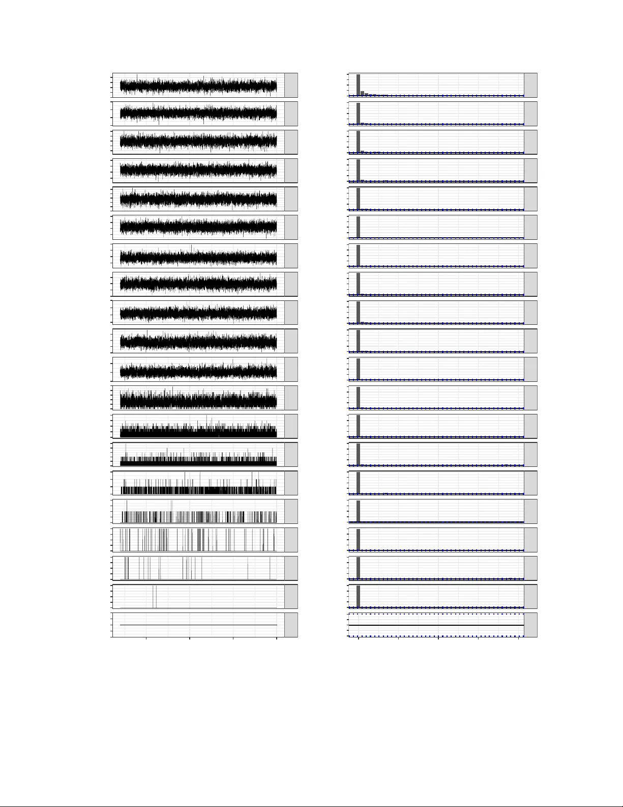
d-blink : Distributed End-to-End Ba y esian En tit y Resolution Neil G. Marc han t a Andee Kaplan b Daniel N. Elazar c Benjamin I. P . Rubinstein a Reb ecca C. Steorts d a Sc ho ol of Computing and Information Systems, Univ ersit y of Melb ourne b Departmen t of Statistics, Colorado State Univ ersit y c Metho dology Division, Australian Bureau of Statistics d Departmen t of Statistical Science and Computer Science, Duk e Univ ersit y Principal Mathematical Statistician, United States Census Bureau DRB #: CBDRB-FY20-309 Septem b er 23, 2020 Abstract En tity resolution (ER; also known as record link age or de-duplication) is the pro cess of merging noisy databases, often in the absence of unique identiﬁers. A ma jor adv ancemen t in ER metho dology has b een the application of Bay esian generativ e mo dels, which provide a natural framew ork for inferring laten t en tities with rigorous quan tiﬁcation of uncertaint y . Despite these adv an tages, existing mo dels are sev erely limited in practice, as standard inference algorithms scale quadratically in the num b er of records. While scaling can b e managed b y ﬁtting the mo del on separate blo c ks of the data, such a na ¨ ıv e approac h ma y induce signiﬁcan t error in the p osterior. In this pap er, we propose a principled mo del for scalable Bay esian ER, called “ d istributed B a yesian link age” or d-blink , whic h join tly p erforms blo c king and ER without compromising p osterior correctness. Our approac h relies on several k ey ideas, including: (i) an auxiliary v ariable representation that induces a partition of the entities and records into blo c ks; (ii) a method for constructing w ell-balanced blo cks based on k-d trees; (iii) a distributed partially-collapsed Gibbs sampler with improv ed mixing; and (iv) fast algorithms for performing Gibbs up dates. Empirical studies on six data sets—including a case study on the 2010 Decennial Census—demonstrate the scalabilit y and eﬀectiveness of our approach. Keywor ds: auxiliary v ariable, distributed computing, Marko v chain Mon te Carlo, partially- collapsed Gibbs sampling, record link age 1 1 INTR ODUCTION When information about a statistical p opulation is scattered across multiple databases, there may b e immense v alue in com bining them. A combined database can provide a more accurate and complete view of the p opulation b y improving cov erage, bringing together analytic v ariables, and resolving erroneous and missing v alues. This allows statisticians to dra w richer and more reliable conclusions. Among the types of questions that can b e addressed b y combining such databases are the follo wing: Ho w accurate are census en umerations for minorit y groups ( Winkler , 2006 )? Ho w many of the elderly are at high risk for sepsis in diﬀerent parts of the coun try ( Saria , 2014 )? How man y p eople were victims of w ar crimes in recen t conﬂicts in Syria ( Price et al. , 2013 )? An imp ortan t step when combining databases is identifying records that refer to the same statistical unit. This is challenging in practice b ecause consisten t identiﬁers, such as so cial security num b ers, are often not av ailable. Iden tiﬁers ma y b e omitted due to priv acy concerns, they may b e inconsisten t across the databases, or they may hav e never b een recorded. In such cases, practitioners m ust rely on entity r esolution (ER) to infer the relationships b et w een records and statistical units (entities) using linking v ariables in the observ ed data. This problem is studied in the statistics, mac hine learning, database and natural language pro cessing communities, and is also known as en tity disam biguation, merge-purge, record link age, deduplication and co-reference resolution ( Christen , 2012b ; Dong and Sriv astav a , 2015 ; So on et al. , 2001 ). ER is not only a crucial to ol for statistical analysis, it is also a challenging statistical and computational problem in itself. This is b ecause man y databases lack reliable linking v ariables, the record comparison space scales quadratically in the n um b er of records, and the n um b er of parameters to b e estimated grows with the num b er of records ( Herzog et al. , 2007 ; Lahiri and Larsen , 2005 ; Winkler , 1999 , 2000 ). T o meet presen t and near-future needs, ER metho ds m ust b e ﬂexible and scalable to large databases. F urthermore, they m ust b e able to handle uncertain ty and b e easily in tegrated with p ost-ER statistical analyses, such as regression. All of this must b e done while achieving lo w error rates. Ba y esian mo dels oﬀer a promising framework for ER as they supp ort natural uncertaint y propagation, ﬂexible mo deling assumptions, and incorp oration of prior information. How ever, existing Bay esian ER mo dels either ignore scalability ( Steorts , 2015 ; Zanella et al. , 2016 ; Sadinle , 2017 ) or manage scalability in an unprincipled manner by applying blo c king outside the Bay esian framework ( F ortini et al. , 2001 ; Larsen , 2005 , 2012 ; T ancredi and Liseo , 2011 ; Gutman et al. , 2013 ; Sadinle , 2014 ; Steorts et al. , 2016 ). Blo cking improv es scalabilit y b y partitioning records in to blo c ks and assuming records in diﬀerent blo c ks do not refer to the same entit y ( Christen , 2012a ). Ho wev er, when blo c king is p erformed as a separate deterministic step it is not p ossible to propagate the uncertaint y . Moreo ver, since the blo c ks are ﬁxed, a p o or blo c king design may compromise the accuracy of the entire ER pro cess. In other words, one sacriﬁces uncertaint y propagation and accuracy for scalability . In this pap er, we prop ose a principled approac h to scaling Bay esian ER mo dels, whic h do es not suﬀer from the limitations of ad-ho c deterministic blo c king. Using the blink ER mo del ( Steorts , 2015 ) as a foundation, w e prop ose a scalable and distributed extension called “ d istributed blink ” or d-blink for short, which in tegrates probabilistic blo c king in 2 a fully Ba y esian framework. T o our kno wledge, d-blink is the ﬁrst Bay esian ER mo del whic h supp orts propagation of uncertain t y b etw een the blo cking and matc hing/linking stages of ER, without compromising the correctness of the p osterior. In addition, d-blink supp orts distributed/parallel inference at the blo c k level to further impro v e scalability to large databases. W e make sev eral con tributions to the literature. First, w e prop ose an auxiliary v ariable represen tation of blink , whic h induces a partitioning of the entities and records into blo cks. These pla y a similar role as traditional deterministic blo c ks, ho wev er the assignments of laten t entities and records to blo c ks are r andom and inferred jointly with the other mo del parameters. Second, w e prov e that our auxiliary v ariable representation preserves the marginal p osterior distribution o ver the mo del parameters. This is a desirable prop ert y , as it means our inferences are theoretically indep enden t of the blo c king design. Third, we prop ose a metho d for constructing well-balanced blo cks based on k -d trees. F ourth, w e design a distributed partially-collapsed Gibbs sampler to p erform inference, and demonstrat e sup erior mixing times when compared to a standard Gibbs sampler. Fifth, w e prop ose algorithms for improving computational eﬃciency of the Gibbs up dates whic h leverage indexing data structures and a nov el p erturbation sampling algorithm. W e implement our prop osed metho dology as an op en-source Apache Spark pac k age 1 and provide an R interface for broad accessibility 2 . W e conduct empirical ev aluations on t wo syn thetic and three real data sets, demonstrating eﬃciency gains in excess of 300 × compared to blink . T o illustrate the eﬀectiveness of our approac h for realistic ER tasks, w e presen t a case study using Census and administrativ e data from the U.S. state of Wy oming. The pap er is organized as follo ws. In Section 2 w e review related w ork in ER metho dology and appro ximate inference algorithms. W e then formulate ER in a Bay esian setting in Section 3 , and present the d-blink mo del with integrated probabilistic blocking. In Section 4 w e provide guidelines for selecting blo c king functions. W e then discuss inference and prop ose a distributed partially-collapsed Gibbs sampler in Section 5 . W e suggest additional metho ds for improving computational eﬃciency of inference in Section 6 . Section 7 provides a comprehensiv e empirical ev aluation, and Section 8 presents a case study to U.S. Census and administrative data. W e mak e closing remarks in Section 9 . 2 RELA TED WORK W e review related work across three main areas—ER metho dology , inference for Bay esian ER mo dels, and distributed Marko v c hain Monte Carlo (MCMC). En tit y resolution metho dology . The ﬁrst probabilistic approach to ER w as due to New combe et al. ( 1959 ), who applied matching rules to pairs of records. This idea was later formalized in a seminal pap er by F ellegi and Sunter ( 1969 ) within a decision-theoretic framew ork. Many v ariations of the F ellegi-Sunter (FS) approac h ha v e b een prop osed (for surv eys, see Winkler , 2006 , 2014 ), including a generalization to m ultiple databases ( Sadinle 1 Spark pac k age source code a v ailable at https://github.com/cleanzr/dblink . 2 R pac k age source code a v ailable at https://github.com/cleanzr/dblinkR . 3 and Fienberg , 2013 ). Others hav e addressed scalability of FS-type approac hes using blo c king/indexing metho ds (see Christen , 2012b ; Steorts et al. , 2014 for surveys) and eﬃcien t data structures ( Enamorado et al. , 2019 ). How ever, traditional FS approac hes do not naturally supp ort propagation of ER uncertaint y , and existing metho ds for scaling make appro ximations that sacriﬁce accuracy . While the FS approach has b een highly inﬂuential, it has also b een criticized due to its lac k of supp ort for duplicates within databases; missp eciﬁed indep endence assumptions; and its dep endence on sub jectiv e thresholds ( T ancredi and Liseo , 2011 ). These limitations hav e prompted dev elopment of more sophisticated Ba yesian mo dels, including mo dels for bipartite matc hing ( F ortini et al. , 2001 ; Larsen , 2005 , 2012 ; T ancredi and Liseo , 2011 ; Gutman et al. , 2013 ; Sadinle , 2017 ; McV eigh et al. , 2019 ), deduplication ( Sadinle , 2014 ; T ancredi et al. , 2020 ) and matching across multiple databases ( Steorts , 2015 ; Steorts et al. , 2016 ). Several of these mo dels op erate on attribute-level comparisons b et wee n pairs of records in a similar v ein as the FS approac h ( Larsen , 2005 , 2012 ; Gutman et al. , 2013 ; Sadinle , 2014 , 2017 ; McV eigh et al. , 2019 ). This contrasts with entit y-centric generative mo dels whic h assume the records arise as distortions to some latent en tity attributes ( T ancredi and Liseo , 2011 ; Steorts , 2015 ; Steorts et al. , 2016 ; T ancredi et al. , 2020 ). In scenarios where training data is scarce or una v ailable, Ba yesian generative mo dels tend to b e more robust than discriminativ e or lik eliho o d-based metho ds, as the priors ha ve a regularizing eﬀect. Ba yesian generativ e models are also amenable to theoretical analysis: recent w ork has obtained lo wer b ounds on the probabilit y of misclassifying the en tit y asso ciated with a record ( Steorts et al. , 2017 ). Ho wev er, a ma jor do wnside of Bay esian ER mo dels is the computational cost of p erforming inference (see discussion b elow). Apart from these adv ances in Bay esian mo dels for ER (largely undertaken in statistics), there hav e b een an abundance of contributions from the database and machine learning com- m unities (see surv eys b y Geto or and Machana v a jjhala , 2012 ; Christen , 2012b ). Their fo cus has typically b een on rule-based approac hes ( F an et al. , 2009 ; Singh et al. , 2017 ), sup ervised learning approac hes ( Mudgal et al. , 2018 ), h ybrid h uman-machine approac hes ( W ang et al. , 2012 ; Gokhale et al. , 2014 ), and scalability ( P apadakis et al. , 2016 ). Broadly sp eaking, all of these approaches rely on either h umans in-the-lo op or large amounts of lab elled training data, which is not generally the case in the Bay esian setting. Inference for Ba y esian ER mo dels. Most prior w ork on Bay esian generativ e mo dels for ER (e.g. T ancredi and Liseo , 2011 ; Gutman et al. , 2013 ; Steorts , 2015 ) has relied on Gibbs sampling for inference. Compared to other Mark ov c hain Mon te Carlo (MCMC) algorithms, Gibbs sampling is relatively easy to implement, how ever it ma y suﬀer from slow con v ergence and p o or mixing o wing to its highly lo cal mov es ( Liu , 2004 ). Scalabilit y is also a c hallenge, as a na ¨ ıv e Gibbs up date for the link age structure requires all-to-all comparisons b et w een records (or b etw een records and en tities for en tity-cen tric mo dels). This issue is often managed b y applying deterministic blo c king prior to Gibbs sampling, thereby sacriﬁcing accuracy and prop er treatment of uncertain ty ( Larsen , 2005 , 2012 ; T ancredi and Liseo , 2011 ; Gutman et al. , 2013 ; Sadinle , 2014 ). In the broader context of clustering mo dels, the split-mer ge algorithm ( Jain and Neal , 2004 ) has b een prop osed as an alternative to Gibbs sampling. It is a Metrop olis-Hastings 4 algorithm, which tra verses the space of clusterings via prop osals that split individual clusters or merge pairs of clusters. Since m ultiple cluster items are up dated in a single mo ve, it is less susceptible to b ecoming trapp ed in lo cal mo des. Steorts et al. ( 2016 ) applied this algorithm, in com bination with deterministic blo cking, to up date the link age structure in an ER mo del similar to blink . A close relative of the split-merge algorithm is the chap er ones algorithm , whic h w as prop osed for inference in micro clustering mo dels ( Zanella et al. , 2016 ). The c hap erones algorithm is exp ected to b e more eﬃcient, as it preferen tially fo cuses on more lik ely cluster reassignments, through a user-sp eciﬁed biased distribution on the pro duct space of cluster items. How ever, the biased distribution m ust b e designed so that random item pairs can b e drawn eﬃcien tly , without explicitly constructing the pro duct space. More recently , Zanella ( 2020 ) prop osed a general framework for designing informative prop osals in a Metrop olis-Hastings setting, whic h is suited for discrete spaces (e.g. the space of p ossible link age structures). They show that lo c al ly-b alanc e d pr op osals are asymptotically- optimal within the class of p oin t wise informative prop osals, and demonstrate signiﬁcan t impro v ements in eﬃciency when compared to a split-merge-t yp e algorithm. How ever, com- puting a lo cally-balanced prop osal for the link age structure is computationally challenging due to quadratic scaling. This can b e mitigated to some exten t b y running lo cally-balanced up dates within randomly-selected sub-blo c ks of records. Ho wev er to a v oid p o or mixing, care m ust b e taken to ensure that randomly-selected sub-blo c ks con tain likely matching records. In con trast to muc h of the literature on Bay esian ER mo dels, McV eigh et al. ( 2019 ) prop osed a metho d that combines deterministic blocking and restricted MCMC (based on earlier w ork b y McV eigh and Murray , 2017 ). They balance appro ximation error b y p erforming coarse-grained deterministic blo cking/indexing as an initial step, follow ed by data-dep enden t p ost-ho c blo c king. During inference, the link age structure is up dated using lo cally-balanced prop osals, restricted to the p ost-ho c blo c ks. They demonstrate improv ed scalabilit y—to data sets with sev eral hundred thousand of record—with minimal risk of appro ximation error. How ever, their approach is not directly compatible with distributed inference (see b elo w) and may require mo diﬁcation for use with an entit y-centric mo del. P arallel/distributed MCMC. Recen t literature has fo cused on using parallel and distributed computing to scale up MCMC algorithms, where applications ha ve included Ba y esian topic mo dels ( Newman et al. , 2009 ; Smola and Naray anamurth y , 2010 ; Ahn et al. , 2014 ) and mixture mo dels ( Williamson et al. , 2013 ; Chang and Fisher , 2013 ; Lo vell et al. , 2013 ; Ge et al. , 2015 ). W e review the application to mixture models, as they are conceptually similar to ER mo dels. Existing work has concen trated on Diric hlet pro cess (DP) mixture mo dels and hierarc hical DP mixture mo dels. The k ey to enabling distributed inference for these mo dels is the realization that a DP mixture mo del can b e reparameterized as a mixture of DPs. Put simply , the reparameterized mo del induces a p artitioning of the clusters into blo c ks, such that clusters assigned to distinct blo cks are conditionally indep enden t. As a result, v ariables within blo cks can b e up dated in parallel. Williamson et al. ( 2013 ) exploited this idea at the thread level to parallelize inference for a DP mixture mo del. Chang and Fisher ( 2013 ) follo w ed a similar approach, but included an additional lev el of parallelization within blo cks 5 using a parallelized version of the split-merge algorithm. Others ( Lo vell et al. , 2013 ; Ge et al. , 2015 ) ha v e dev elop ed distributed implementations in the MapReduce framework. W e do not consider DP mixture mo dels in our w ork, as their b ehavior is ill-suited for ER applications. 3 Ho wev er w e do b orro w the reparameterization idea, alb eit with a more ﬂexible partition sp eciﬁcation whic h p ermits similar en tities to b e co-blo c k ed, while facilitating load balancing. It would b e in teresting to see whether similar ideas can b e applied to micro clustering mo dels ( Zanella et al. , 2016 ), how ever preserving the marginal p osterior distribution seems challenging in this case. 3 A SCALABLE MODEL F OR BA YESIAN ER In this section, w e present our scalable ER mo del called d-blink , which in tegrates proba- bilistic blo cking in a fully Bay esian framew ork. Our mo del can b e viewed as an extension of the blink mo del ( Steorts , 2015 ) that incorp orates an auxiliary partition of the latent en tit y parameter space in to blo c ks. Unlike ad-ho c blo c king approac hes used previously in the literature ( Larsen , 2005 , 2012 ; T ancredi and Liseo , 2011 ; Gutman et al. , 2013 ; Sadinle , 2014 ; Steorts et al. , 2016 ), the blo c ks in d-blink are random, and inferred jointly with the other mo del parameters. This enables propagation of uncertaint y b etw een the blo cking and ER stages. In addition, d-blink extends blink with supp ort for missing v alues and user-deﬁned attribute similarity measures. W e describ e notation and assumptions in Section 3.1 , b efore presenting d-blink in Section 3.2 . W e deﬁne attribute similarity measures in Section 3.3 , including an optional truncation appro ximation whic h can impro ve scalability . In Section 3.4 , we prov e that the marginal posterior of d-blink (in tegrated o ver the blo c ks) reduces to blink under certain conditions. This is a desirable prop ert y , as it means our inferences are theoretically indep enden t of the blo cking design. Finally , in Section 3.5 we explain how the auxiliary blo c ks are b eneﬁcial in scaling and distributing inference. 3.1 Notation and problem form ulation In this section, w e deﬁne notation and form ulate ER in a Bay esian setting. Consider a collection of T tables 4 (databases) indexed b y t , eac h with R t records (rows) indexed b y r and A aligned attributes (columns) indexed b y a . Asso ciated with the records is a ﬁxed p opulation of entities of size E indexed by e . Each en tity e is describ ed by a set of attributes y e = [ y ea ] a =1 ...A , which are aligned with the record attributes. The p opulation of entities is partitioned into B blo c ks for computational conv enience, using a blo cking function BlockFn that maps an entit y e to a blo c k based on its attributes y e . W e assume eac h record ( t, r ) b elongs to a blo c k γ tr and is asso ciated with an entit y λ tr within that blo c k. The v alue of the a -th attribute for record ( t, r ) is denoted by x tra , and is assumed to b e a noisy observ ation of the associated en tity’s true attribute v alue y λ tr a . W e allow 3 With a DP prior, the num b er of clusters grows logarithmically in the num b er of records, but empirical observ ations call for near-linear growth ( Zanella et al. , 2016 ). 4 W e deﬁne a table as an ordered (indexed) collection of records, which may con tain duplicates (records for whic h all attributes are iden tical). 6 for the fact that some attributes x tra ma y b e missing completely at random through a corresp onding indicator v ariable o tra ( Little and Rubin , 2002 , p. 12). T able 1 summarizes our notation, including mo del-sp eciﬁc parameters whic h will b e in tro duced shortly . W e adopt the following rules to compactly refer to sets of v ariables: • A b oldface low er-case v ariable denotes the set of al l attributes : e.g. x tr = [ x tra ] a =1 ...A . • A b oldface capital v ariable denotes the set of al l index c ombinations : e.g. X = [ x tra ] t =1 ...T ; r =1 ...R t ; a =1 ...A . W e also deﬁne notation to separate the record attributes X in to an observ ed part X ( o ) (those x tra ’s for which o tra = 1) and a missing part X ( m ) (those x tra ’s for which o tra = 0). After sp ecifying a generative mo del (see next section), w e p erform ER b y inferring the joint p osterior distribution o ver: • the blo ck assignmen ts Γ = [ γ tr ] t =1 ...T ; r =1 ...R t , • the link age structure Λ = [ λ tr ] t =1 ...T ; r =1 ...R t , and • the true entit y attribute v alues Y = [ y ea ] e =1 ...E ; a =1 ...A , conditional on the observ ed record attribute v alues X ( o ) . Note that w e op erate in a fully unsup ervised setting, since we do not condition on ground truth data for the links or entities. Inferring Γ is equiv alent to the blo cking stage of ER, where the records are partitioning in to blo c ks to limit the comparison space. Inferring Λ is equiv alent to the matching/linking stage of ER, where records that refer to the same entities are linked together. Inferring Y is equiv alent to the mer ging stage, where link ed records are combined to pro duce a single represen tativ e record. By inferring Γ , Λ and Y join tly , we are able to propagate uncertain t y b et w een the three stages. 3.2 Mo del sp eciﬁcation W e now presen t our prop osed mo del d-blink b y describing the generative pro cess. W e pro vide a visual representation of the mo del in Figure 1 , with k ey diﬀerences from blink highligh ted in a dashed blue line st yle. En tities. The p opulation of entities is assumed to b e of ﬁxed size E . Eac h entit y e is describ ed by a vector of “true” attributes y e ∈ N A a =1 V a . The v alue of the a -th attribute y ea is assumed to b e drawn indep enden tly from a distribution φ a o v er the attribute domain V a : y ea ind . ∼ Discrete v ∈V a [ φ a ( v )] . (1) F ollowing the blink mo del, we set the p opulation size E and the distributions o ver the attribute domains φ a empirically . Recommendations for setting these parameters are pro vided in App endix F.3 . 7 α a θ ta β a z tra x tra λ tr γ tr y ea φ a E b η ta o tra E R t T B A Figure 1: Plate diagram for d-blink . Extensions to blink are highlighted in a dashed blue line style. Circular no des represen t random v ariables; square no des represent deterministic v ariables; (un)shaded no des represen t (un)observ ed v ariables; arrows represent conditional dep endence; and plates represent replication ov er an index. T able 1: Summary of notation. Sym b ol Description Sym b ol Description t ∈ 1 . . . T index o ver tables γ tr assigned block for record r in table t r ∈ 1 . . . R t index o ver records in table t λ tr assigned en tit y for record r in table t e ∈ 1 . . . E index o ver en tities θ ta prob. attribute a in table t is distorted b ∈ 1 . . . B index ov er blo c k α a , β a distortion h yp erparams. for attribute a a ∈ 1 . . . A index o ver attributes η ta prob. attribute a in table t is observed v ∈ 1 . . . |V a | index o ver domain of attribute a V a domain of attribute a R = P t R t total n umber of records φ a ( · ) distribution o ver domain of attribute a x tra attribute a for record r in table t sim a ( · , · ) similarit y measure for attribute a z tra distortion indicator for x tra R e set of records assigned to en tit y e o tra observ ed indicator for x tra E b set of entities assigned to blo c k b y ea attribute a for entit y e BlockFn ( · ) blo c k assignmen t function 8 Blo c ks. The parameter space asso ciated with the entities N A a =1 V a is partitioned into B blo c ks. The partition is parameterized using a deterministic blo cking function : BlockFn : O a V a → { 1 , . . . , B } , (2) whic h is a free parameter and may be selected for inferen tial conv enience. W e pro vide recommendations for selecting the blo cking function in Section 4 , including an example based on k -d trees. W e shall often need to refer to the entities assigned to a particular blo ck. T o do this concisely , w e introduce the notation E b ( Y ) = { e : BlockFn ( y e ) = b } to denote the set of en tities assigned to blo ck b . This is random due to the dep endence on Y , how ever we shall often omit the dep endence for brevit y . Distortion. Asso ciated with each table t and attribute a is a distortion probability θ ta , with assumed prior distribution: θ ta | α a , β a ind . ∼ Beta[ α a , β a ] , (3) where α a and β a are hyperparameters. W e pro vide recommendations for setting α a and β a in App endix F . The distortion probabilities feed into the record-generation pro cess b elow. Records. W e assume a record is generated b y selecting an entit y uniformly at random and copying the en tity’s attributes sub ject to distortion. The pro cess for generating record r in table t is outlined b elo w. Steps (i), (ii), and (v) deviate from blink . (i) Cho ose a blo c k assignment γ tr at random in prop ortion to the blo ck sizes: γ tr | Y ind . ∼ Discrete b ∈{ 1 ...B } [ |E b | /E ] . (4) (ii) Cho ose an en tity assignmen t λ tr uniformly at random from blo ck γ tr : λ tr | γ tr , Y ind . ∼ DiscreteUniform[ E γ tr ] . (5) (iii) F or each attribute a , dra w a distortion indicator z tra : z tra | θ ta ind . ∼ Bernoulli[ θ ta ] . (6) (iv) F or each attribute a , dra w a record v alue x tra : x tra | z tra , y λ tr a ind . ∼ (1 − z tra ) δ ( y λ tr a ) + z tra Discrete v ∈V a [ ψ a ( v | y λ tr a )] (7) where δ ( · ) represents a p oint mass. If z tra = 0, x tra is copied directly from the entit y . Otherwise, x tra is drawn from the domain V a according to the distortion distribution ψ a . In the literature, this is kno wn as a hit-miss mo del ( Copas and Hilton , 1990 ). (v) F or each attribute a , dra w an observed indicator o tra : o tra ind . ∼ Bernoulli[ η ta ] . (8) If o tra = 1, x tra is observed, otherwise it is missing. 9 Detail on the distortion distribution. ψ a ( ·| w ) chooses a distorted v alue for attribute a conditional on the true v alue w . In our parameterization of the mo del, it is deﬁned as ψ a ( v | w ) = h a ( w ) φ a ( v )e sim a ( v ,w ) , (9) where h a ( w ) = 1 / P v ∈V a φ a ( v )e sim a ( v ,w ) is a normalization constan t and sim a is the similarit y measure for attribute a (see Section 3.3 ). In tuitiv ely , this distribution chooses v alues in prop ortion to their empirical frequency , while placing more weigh t on those that are “similar” to w . This reﬂects the notion that distorted v alues are likely to b e close to the truth, as is the case when mo deling typographical errors. P osterior distribution. The generative pro cess describ ed ab ov e corresp onds to a p oste- rior distribution o v er the model parameters, conditioned on the observ ed records. By reading the conditional dep endence structure oﬀ the plate diagram (Figure 1 ) and marginalizing o v er the missing record attributes X ( m ) , one can sho w that the p osterior distribution is of the following form: p ( Γ , Λ , Y , Z , Θ | X ( o ) , O ) ∝ Y e,a p ( y ea | φ a ) × Y t,a p ( θ ta | α a , β a ) × Y t,r,a o tra =1 p ( x tra | z tra , λ tr , y λ tr a ) × Y t,r n p ( γ tr | Y ) p ( λ tr | γ tr , Y ) Y a p ( z tra | θ ta ) o . (10) F or further detail on the deriv ation and an expanded form of the p osterior, w e refer the reader to App endix A . 3.3 A ttribute similarit y measures W e now discuss the attribute similarity measures that app ear in the distortion distribution of Equation 9 . The purp ose of these measures is to quantify the prop ensit y that some v alue v in the attribute domain is chosen as a distorted alternativ e to the true v alue w . Deﬁnition (A ttribute similarit y measure) . L et V b e the domain of an attribute. A n attribute similarity measure on V is a function sim : V × V → [0 , s max ] that satisﬁes 0 ≤ s max < ∞ and sim ( v , w ) = sim ( w , v ) for al l v , w ∈ V . Note that our parameterization in terms of attribute similarity measures diﬀers from blink , which uses distanc e measures. This allo ws us to make use of a more eﬃcient sampling metho d, as describ ed in Section 6.3 . The next prop osition states that the tw o parameterizations are equiv alent, so long as the distance measure is b ounded and symmetric (a pro of is provided in App endix B.1 ). Prop osition 1. L et dist a : V × V → [0 , d max; a ] b e the attribute distanc e me asur e that app e ars in blink , and assume that 0 ≤ d max; a < ∞ and dist a ( v , w ) = dist a ( w , v ) for al l v , w ∈ V . Deﬁne the c orr esp onding attribute similarity me asur e for d-blink as sim a ( v , w ) := d max; a − dist a ( v , w ) . (11) Then the p ar ameterization of ψ a use d in d-blink is e quivalent to blink . 10 In this pap er, we restrict our attention to the following similarit y measures for simplicity: • Constant similarity me asur e. This measure is appropriate for categorical attributes, where there is no reason to b eliev e one v alue is more likely than an y other as a distortion to the true v alue w . Without loss of generality , it may b e deﬁned as sim const ( v , w ) = s max for all v , w ∈ V . • Normalize d e dit similarity me asur e. This measure is based on the edit distance metric, and is suitable for mo deling distortion in generic string attributes. F ollowing Y ujian and Bo ( 2007 ), w e deﬁne a normalized edit distance metric, dist nEd ( v , w ) = 2 dist Ed ( v , w ) | v | + | w | + dist Ed ( v , w ) , where dist Ed denotes the regular edit distance and | v | denotes the length of string v . Note that alternative deﬁnitions of the normalized edit distance could b e used (see references in Y ujian and Bo , 2007 ), how ever the ab ov e deﬁnition is unique in that it yields a prop er metric. Since the normalized edit distance is b ounded on the interv al [0 , 1] we can deﬁne a corresp onding normalized edit similarity measure: sim nEd ( v , w ) = 1 − dist nEd ( v , w ) . (12) Ideally , one should select attribute similarity measures based on the data at hand. There are man y p ossibilities to consider, suc h as Jaccard similarity , n umeric similarity measures ( Lesot et al. , 2008 ) and other domain-sp eciﬁc measures ( Bilenko and Mo oney , 2003 ). 3.4 Mo del equiv alence W e hav e purp osely constructed d-blink so that it reduces to blink under certain conditions. Assuming the records are fully observ ed, the p osterior distribution of d-blink as sp eciﬁed in Equation 10 is similar to blink . The diﬀerence lies in the factors inv olving the blo c k assignmen ts γ tr and the entit y assignments λ tr . Ho wev er, if one marginalizes out the auxiliary blo ck assignments—as is done automatically in Marko v c hain Mon te Carlo—the p osterior distributions are iden tical. This statemen t is made precise b elow (pro of provided in App endix B.2 ): Prop osition 2. Supp ose the c onditions of Pr op osition 1 hold and that α a = α and β a = β for al l a . Assume furthermor e that al l r e c or d attributes ar e observe d, i.e. o tra = 1 for al l t, r , a . Then the mar ginal p osterior of Λ , Y , Z and Θ for d-blink (i.e. mar ginalize d over Γ = [ γ tr ] t =1 ...T ; r =1 ...R t ) is identic al to the p osterior for blink . This is an imp ortan t result, as it shows our inferences for the meaningful mo del parame- ters are the same as w e would obtain from blink . Thus we are able to apply blo cking to scale the mo del, without compromising the correctness of the p osterior distribution. 11 3.5 Rationale for in tro ducing blo c k W e no w brieﬂy explain the role of the auxiliary blo c k in d-blink . First, w e note that without the blo ck ( B = 1), the Marko v blanket for λ tr includes the attribute v alues for al l of the entities Y . This presen ts a ma jor obstacle when it comes to distributing the inference on a compute cluster, as the data is not separable. By incorp orating blo ck, w e restrict the Mark ov blanket for λ tr to include only a subset of the entit y attribute v alues—those in the same blo c k as record ( t, r ). As a result, it b ecomes natural to distribute the inference so that each compute no de is resp onsible for a single block (see Section 5.2 for details). Secondly , we can interpret the blo c k as p erforming probabilistic blo c king in the context of MCMC sampling (introduced in Section 5 ), which improv es computational eﬃciency . In a giv en iteration, the p ossible links for a record are restricted to the entities residing in the same blo c k. How ever, unlike con v entional blo cking, the blo c k assignments are not ﬁxed—b et w een iterations the en tities and linked records may mov e b etw een blo c ks. 4 BLOCKING FUNCTIONS In Section 3.2 we introduced a generic blo c king function (Equation 2 ) that is resp onsible for assigning entities to blo c ks. This function may b e regarded as a free parameter, since it has no b earing on mo del equiv alence according to Prop osition 2 . How ev er, from a practical p ersp ectiv e the blo c king function ought to b e c hosen carefully , as it can impact inferential eﬃciency—b oth in terms of computational and mixing time. W e suggest some guidelines for choosing a blo c king function in Section 4.1 , b efore presen ting an example based on k -d trees in Section 4.2 . 4.1 In terpretation and guidelines Recall that the blo cking function assigns an en tity to a blo ck according to its attributes y e = [ y ea ] a =1 ...A . Since y e is unobserve d , it must b e treated as a random v ariable ov er the space of p ossible attributes V ⊗ := N A a =1 V a . This means the blo c king function should not b e in terpreted as partitioning the entities directly . Rather, it should b e interpreted as partitioning the space V ⊗ in which the en tities reside, while taking the distribution ov er V ⊗ in to accoun t. With this in terpretation in mind, we argue that the blo cking function should ideally satisfy the follo wing prop erties: (i) Balanc e d weight. The blo c ks should ha v e equal weigh t (probabilit y mass) under the distribution ov er V ⊗ , thereb y ensuring the en tities are distributed evenly (in exp ectation) among the blo c ks. This is a desirable prop ert y , as it ensures prop er load balancing for our distributed inference algorithm (see Section 5.2 ). (ii) Entity sep ar ation. A pair of en tities drawn at random from the same blo c k should ha v e a high degree of similarity , while entities drawn from diﬀeren t blo cks should hav e a low degree of similarit y . This improv es the likelihoo d that similar records will end up in the same blo ck, and allows them to more readily form lik ely en tities. 12 These prop erties need not b e satisﬁed strictly: the extent to whic h they are satisﬁed is merely exp ected to improv e the eﬃciency of the inference. F or example, satisfying the ﬁrst prop ert y requires kno wledge of the marginal p osterior distribution o ver y e , which is infeasible to calculate. W e note that there is likely to b e tension b et ween the tw o prop erties, so that a balance must b e struck b et ween them. 4.2 Example: k -d tree blo c king function W e now describ e a blo cking function based on k -d trees, whic h is used in our exp eriments in Section 7 . Bac kground. A k -d tree is a binary tree that recursively partitions a k -dimensional aﬃne space ( Bentley , 1975 ; F riedman et al. , 1977 ). In the standard set-up, eac h no de of the tree is asso ciated with a data p oin t that implicitly splits the input space into t w o half-spaces along a particular dimension. Owing to its ability to hierarchically group nearby p oin ts, it is commonly used to sp eed up nearest-neighbor search. This makes a k -d tree a go o d candidate for a blo c king function, since it can b e balanced while grouping similar p oin ts. Setup. Our setup diﬀers from a standard k -d tree in several asp ects. First, we consider a discrete space V ⊗ (not an aﬃne space), where the “ k dimensions” are the A attributes. Second, we do not store data p oin ts in the tree. W e only require that the tree implicitly stores the b oundaries of the blo c ks, so that it can assign an arbitrary y ∈ V ⊗ to the correct partition (a leaf no de). Finally , since w e are w orking in a discrete space, the input space to a no de is a coun table set. The no de must split the input set into tw o parts based on the v alues of one of the attributes. Fitting the tree. Since it is infeasible to calculate the marginal p osterior distribution o v er y e exactly , we use the empirical distribution from the tables as an approximation. As a result, we treat the records (tables) as a sample from the distribution o ver y e , and ﬁt the tree so that it remains balanced with resp ect to this sample. The depth of the tree d determines the num b er of blo c ks (2 d ). Ac hieving balanced splits. When ﬁtting the tree, eac h no de receives an input set of samples and a rule must b e found that splits the set into tw o roughly equal (balanced) parts based on an attribute. W e consider t wo types of splitting rules: the or der e d me dian and the r efer enc e set (see App endix C ). W e allow the practitioner to sp ecify an ordered list of attributes to b e used for splitting. T o ensure balanced splits, we recommend selecting attributes with a large domain. If p ossible, we recommend preferencing attributes which are known a priori to b e reliable (low distortion), as this will reduce the shuﬄing of en tities/ records b etw een blo c ks. In principle, it is p ossible to automate the pro cess of ﬁtting a tree: one could grow several trees with randomly-selected splits and use the one that is most balanced. W e examine balance empirically in App endix H . 13 5 INFERENCE W e no w turn to approximating the full join t p osterior distribution o ver the unobserved v ariables Z , Y , Θ , Γ and Λ , as given in Equation 10 . Since it is infeasible to sample from this distribution directly , we design MCMC algorithms based on partially-collapsed Gibbs (PCG) sampling ( v an Dyk and P ark , 2008 ). In addition, w e show ho w to exploit the conditional indep endence induced by the blo c ks to distribute the PCG sampling across m ultiple threads or mac hines. 5.1 P artially-collapsed Gibbs sampling F ollowing the blink pap er ( Steorts , 2015 ), we initially exp erimented with regular Gibbs sampling. 5 Ho wev er, the resulting Mark o v c hains exhibited slo w conv ergence and po or mixing. This is a kno wn shortcoming of Gibbs sampling whic h ma y b e remedied b y collapsing v ariables and/or up dating correlated v ariables in groups ( Liu , 2004 ). These ideas form the basis for a framework called p artial ly-c ol lapse d Gibbs (PCG) sampling —a generalization of Gibbs sampling that has b etter con vergence prop erties ( v an Dyk and P ark , 2008 ). Under the PCG framew ork, v ariables are up dated in groups b y sampling from their conditional distributions. These conditional distributions ma y b e taken with resp ect to the join t p osterior (like regular Gibbs), or with resp ect to mar ginal distributions of the joint p osterior (unique to PCG). The latter case is called trimming and must b e handled with care so as not to alter the stationary distribution of the Marko v chain. In applying PCG sampling to d-blink , we m ust decide how to apply the three to ols: mar ginalization (equiv alent to grouping), p ermutation (changing the order of the up dates) and trimming (removing marginalized v ariables). In theory , the conv ergence rate should impro ve with more marginalization and trimming, ho wev er this m ust be balanced with the following: (i) whether the resulting conditionals can b e sampled from eﬃciently , and (ii) whether the resulting dep endence structure is compatible with our distributed set-up (see Section 5.2 ). W e consider tw o samplers, PCG-I and PCG-I I, describ ed b elo w. Of the tw o, we recommend PCG-I as it is more eﬃcien t in our empirical ev aluations (see Section 7.1 ). W e include the PCG-I I sampler, as one would exp ect the PCG-I I sampler to p erform b etter than the PCG-I sampler in terms of mixing, how ever when computational eﬃciency is taken into accoun t the p erformance is w orse (see Figure 6 ). 5.1.1 PCG-I sampler The PCG-I sampler uses regular Gibbs up dates for θ ta , λ tr and z tra for all t , r and a . The conditional distributions for these up dates are listed in App endix D . When up dating the en tit y attributes y ea and the blo ck assignments γ tr , marginalization and trimming are used. Sp eciﬁcally , w e apply marginalization by join tly up dating y e and { γ tr , z tr } R e (the set of γ tr ’s and z tr ’s for records ( t, r ) linked to entit y e ). W e then trim (analytically integrate o v er) { z tr } R e . 5 W e deﬁne r e gular Gibbs sampling as the most basic v ariation where v ariables are updated iteratively one-at-a-time b y sampling from their conditional distributions. 14 Step 1 Step 2 Step 3 Step 4 Update Θ on the manager and broadcast to the wo rkers. Θ Update Λ on the w ork ers. Records ma y only link to entities within their assigned blo cks. Update Y and Γ on the wo rkers. Then move the entities and records to their newly-assigned blo cks. Update Z , then calculate summary stats on the wo rkers. Broadcast to the manager. stats stats Θ Figure 2: Sc hematic depicting a single iteration of distributed PCG sampling. The entit y attributes ( Y —circular no des), record attributes and their distortion indicators ( X , Z — square no des), and links from records to en tities ( Λ —no de connectors) are distributed across the work ers (blue rectangular plates) according to their assigned blo cks. The distortion probabilities ( Θ ) reside on the manager (green rounded-rectangular plate). W e shall now derive this up date. Referring to Equation 10 , the joint p osterior of y e , { γ tr , z tr } R e conditioned on the other parameters has the form p  y e , { γ tr , z tr } R e   Z ¬R e , Γ ¬R e , Θ , Λ , X ( o ) , O  ∝ Y a n p ( y ea | φ a ) × Y ( t,r ) ∈R e p ( γ tr | Y ) p ( λ tr | γ tr , Y ) p ( z tra | θ ta ) × Y ( t,r ) ∈R e o tra =1 p ( x tra | z tra , λ tr , y ea ) o , where sup erscript ¬R e denotes exclusion of an y records ( t, r ) ∈ R e (those currently link ed to entit y e ). Substituting the distributions and trimming { z tr } R e yields p  y e , { γ tr } R e   Z ¬R e , Γ ¬R e , Θ , Λ , X ( o ) , O  = p ( { γ tr } R e |R e , y e ) Y a p ( y ea |R e , Θ , X ( o ) , O ) (13) where p ( y ea |R e , Θ , X ( o ) , O ) ∝ φ a ( y ea ) Y ( t,r ) ∈R e o tra =1 { (1 − θ ta ) I [ x tra = y ea ] + θ ta ψ a ( x tra | y ea ) } and p ( { γ tr } R e |R e , y e ) ∝ Y ( t,r ) ∈R e I [ γ tr = BlockFn ( y e )] . Note that the up date for { γ tr } R e is deterministic, conditional on y e and R e . Since we hav e applied trimming, we must p ermute the up dates so that the trimmed v ariables Z are not conditioned on in later up dates. This means the up dates for y e and { γ tr , z tr } R e m ust come after the up dates for θ ta and λ tr , but b efor e the up dates for z tra . 15 T able 2: Dep endencies for the conditional up dates used in the PCG-I sampler. Up date v ariables Dep endencies θ ta z t · a = P r z tra λ tr z tr , x tr , γ tr , E γ tr , { y e } e ∈E γ tr y ea , { γ tr , z tra } ( t,r ) ∈R e R e , { x tra } ( t,r ) ∈R e , { θ ta } ( t,r ) ∈R e z tra x tra , λ tr , y λ tr a , θ ta 5.1.2 PCG-I I sampler The PCG-I I sampler is identical to PCG-I, except that it replaces the regular Gibbs up date for λ tr with an up date that marginalizes and trims z tr . T o deriv e the distribution for this up date, we ﬁrst consider the joint p osterior of λ tr and z tr conditioned on the other parameters: p ( λ tr , z tr | Γ , Y , Θ , Z ¬ ( t,r ) , X ( o ) , O ) ∝ p ( λ tr | γ tr , Y ) × Y a p ( z tra | θ ta ) × Y a o tra =1 p ( x tra | z tra , λ tr , y λ tr a ) where sup erscript ¬ ( t, r ) denotes exclusion of record ( t, r ). Substituting the distributions and trimming z tr yields p ( λ tr | Γ , Y , Θ , Z ¬ ( t,r ) , X ( o ) , O ) ∝ I [ λ tr ∈ E γ tr ( Y )] × Y a o tra =1 n (1 − θ ta ) I [ x tra = y λ tr a ] + θ ta ψ a ( x tra | y λ tr a ) o . (14) 5.2 Distributing the sampling By examining the conditional distributions derived in the previous section and those listed in App endix D , one can show that the up dates for the v ariables asso ciated with entities and records ( z tra , λ tr , γ tr and y ea ) only dep end on v ariables asso ciated with en tities and records assigned to the same blo c k (excluding Θ ). These dep endencies are summarized in T able 2 for the PCG-I sampler. The distortion probability θ ta is an exception—it is not asso ciated with an y blo c k and may dep end on z tra ’s across al l blo c ks. This dep endence structure—in particular, the conditional indep endence of entities and records across blo cks—mak es the PCG sampling amenable to distributed computing. As suc h, we prop ose a manager-work er arc hitecture where: • the manager is resp onsible for storing and up dating v ariables not asso ciated with an y blo c k (i.e. Θ ); and • eac h worker represen ts a blo ck, and is resp onsible for storing and up dating v ariables asso ciated with the entities and records assigned to it. 16 The manager/work ers ma y b e pro cesses running on a single mac hine or on machines in a cluster. If using a cluster, w e recommend that the no des b e tightly coupled, as frequent comm unication b etw een them is required. Figure 2 depicts a single iteration of PCG sampling using our prop osed manager-w ork er arc hitecture. Of the four steps depicted, steps 2 and 3—where the links, entit y attributes and blo ck assignmen ts are up dated—are the most computationally intensiv e. W e therefore exp ect to ac hieve a signiﬁcant sp eed-up by distributing these steps across the w orkers. T o ensure go o d load balancing of these steps it is imp ortan t that the blo c ks are well- balanced (see Section 4.1 ), otherwise work ers resp onsible for smaller blo c ks m ust w ait idly for other work ers to ﬁnish b efore the next iteration can b egin. This is b ecause step 1 requires global sync hronization of state across the work ers. The blo cks also hav e an eﬀect on communication costs, which are most signiﬁcan t in step 3, where the entities and link ed records are sh uﬄed to their newly-assigned blo c ks. A w ell-chosen blo cking function can minimize this cost, b y ensuring similar records/en tities are co-blo ck ed. 6 COMPUT A TIONAL EFFICIENCY CONSIDERA TIONS 6.1 Eﬃcien t pruning of candidate links In this section, we describ e a trick that is aimed at impro ving the computational eﬃciency of the Gibbs up date for λ tr (used in the Gibbs and PCG-I samplers). This particular tric k do es not apply to the joint PCG up date for λ tr and z tr (used in the PCG-I I sampler). Consider the conditional distribution for the λ tr up date in Equation S5 of App endix D : p ( λ tr = e | Γ , Y , Z , X ( o ) , O ) ∝ I [ e ∈ E γ tr ( Y )] × Y a o tra =1 n (1 − z tra ) I [ x tra = y ea ] + z tra ψ a ( x tra | y ea ) o . (15) The supp ort of this distribution is the set of c andidate links for record ( t, r ), whic h we denote b y L tr . Lo oking at the ﬁrst indicator function ab ov e, we see that L tr ⊆ E γ tr , i.e. the candidate links are restricted to the entities in the same blo ck as record ( t, r ). Thus, a na ¨ ıv e sampling approach for this distribution tak es O ( |E γ tr | ) time. W e can impro v e up on the na ¨ ıv e approach by exploiting the fact that L tr is often considerably smaller than E γ tr . T o see wh y this is the case, note that the second indicator function in Equation 15 further restricts L tr if any of the distortion indicators for the observ ed record attributes are zero. Sp eciﬁcally , if z tra = 0 and o tra = 1, L tr cannot contain an y entit y whose a -th attribute y ea do es not match the record’s a -th attribute x tra . This implies L tr is likely to b e small in the case of low distortion. Putting aside the computation of L tr for the momen t, this means w e can reduce the time required to up date λ tr to O ( |L tr | ). T o compute L tr eﬃcien tly , we prop ose main taining an inv erted index o ver the entit y attributes within each blo ck. Sp eciﬁcally , the index for the a -th attribute in blo ck b should accept a query v alue v ∈ V a and return the set of entities that match on v : M pa ( v ) = { n ∈ E p : y ea = v } . (16) 17 0 s cut s max 0 s max sim ( v , w ) sim ( v , w ) Figure 3: T ransformation from a ra w similarit y function ( sim ) to a truncated similarity function ( sim ). Once the index is constructed, w e can eﬃciently retriev e the set of candidate links for record ( t, r ) by computing a m ultiple set intersection: L tr = \ { a : z tra =0 ∧ o tra =1 } M γ tr a ( x tra ) . (17) This assumes at least one of the observ ed record attributes is not distorted. Otherwise L tr = E γ tr . Since the sizes of the sets M γ tr a ( x tra ) are lik ely to v ary signiﬁcantly , w e advise computing the intersection iterativ ely in increasing order of size. That is, we b egin with the smallest set and retain the elements that are also in the next largest set, and so on. With a hash-based set implementation, this scales linearly in the size of the ﬁrst (smallest) set. 6.2 Cac hing and truncation of attribute similarities W e hav e not y et emphasized that the up dates for Λ , Y and Γ dep end on the attribute similarities b et ween pairs of v alues in the attribute domains. Sp eciﬁcally , for each attribute a , we need to access the indexed set S a = { sim a ( v , w ) : v , w ∈ V a × V a } . These similarities ma y b e exp ensive to ev aluate on-the-ﬂy , so we cache the results in memory on the w ork ers. T o manage the quadratic scaling of S a , and in anticipation of another tric k introduced in Section 6.3 , we transform the similarities so that those b elow a cut-oﬀ s cut; a are regarded as completely disagreeing. W e achiev e this by applying the following truncation transformation to the raw attribute similarity sim a ( v , w ): sim a ( v , w ) = max  0 , sim a ( v , w ) − s cut; a 1 − s cut; a /s max; a  . (18) as illustrated in Figure 3 . Whenev er a ra w attribute similarit y is called for, w e replace it with this truncated v ersion. Only pairs of v alues with p ositiv e truncated similarit y are stored in the cac he—those not stored in the cache hav e a truncated similarity of zero b y default. Note that attributes with a constant similarity function sim const are treated sp ecially—there is no need to cache the index set of similarities, since they are all iden tical. It is imp ortan t to ackno wledge that the truncated similarities are an approximation to the original mo del. W e claim that the approximation is reasonable on the follo wing grounds: 18 • L ow loss of information. Below a certain cut-oﬀ, the attribute similarity func- tion is unlikely to encode m uch useful information for mo deling the distortion pro cess. F or example, the fact that sim nEd ( “Smith” , “Chiu” ) = 0 . 385 whereas sim nEd ( “Smith” , “Chen” ) = 0 . 286, do esn’t necessarily suggest that “Chiu” is more lik ely than “Chen” as a distorted alternativ e to “Smith”. • Pr e c e dent. In the record link age literature, v alue pairs with similarities b elo w a cut-oﬀ are regarded as completely disagreeing ( Winkler , 2002 ; Enamorado et al. , 2019 ). • Eﬃciency gains. As w e shall so on see in Section 6.3 , w e can p erform the com bined Y , Γ , Z up date more eﬃcien tly b y eliminating pairs b elo w the cut-oﬀ from consideration. 6.3 F ast up dates of en tity attributes using p erturbation sampling W e now present a no v el sampling algorithm that allo ws us to eﬃcien tly p erform the PCG up date for y ea and { γ tr , z tra } R e . The algorithm relies on the observ ation that the conditional distribution for y ea can b e expressed as a mixture ov er tw o comp onen ts: (i) a b ase distribution o v er V a whic h is ideally constan t for all entities; and (ii) a p erturb ation distribution whic h v aries for each en tity , but has a muc h smaller supp ort than V a . With this representation, we can a v oid computing and sampling from the full distribution o v er V a , which v aries for each y ea up date. Rather, we only need to compute the p erturbation distribution ov er a muc h smaller supp ort, and then sample from the mixture, which can b e done eﬃciently using the V ose-Alias metho d ( V ose , 1991 ). W e refer to this algorithm as p erturb ation sampling . 6.3.1 P erturbation sampling Although we’re in terested in applying p erturbation sampling to a sp eciﬁc conditional distribution, we describ e the idea in generality b elo w. Consider a target probability mass function (pmf ) p ( x | ω ) with ﬁnite supp ort X , which v aries as a function of parameters ω ∈ Ω. In general, one m ust recompute the probability tables to draw a new v ariate whenever ω c hanges—a computation that tak es O ( |X | ) time. Ho w ever, if the dep endence on ω is of a certain restricted form, we show that it is p ossible to achiev e b etter scalabilit y b y expressing the target as a mixture. This is made precise in the following result. Prop osition 3. L et p ( x | ω ) b e a pmf with ﬁnite supp ort X , which dep ends on p ar ameters ω ∈ Ω . Supp ose ther e exists a “b ase” pmf q ( x ) over X which is indep endent of ω and a non-ne gative b ounde d p erturb ation term  ( x | ω ) , such that p ( x | ω ) c an b e factorize d as p ( x | ω ) ∝ q ( x )(1 +  ( x | ω )) . Then p ( x | ω ) c an b e expr esse d as a mixtur e over the b ase pmf q ( x ) and a “p erturb ation ” pmf v ( x | ω ) := c q ( x )  ( x | ω ) over X ? = { x ∈ X :  ( x | ω ) > 0 } as fol lows: p ( x | ω ) = c 1 + c q ( x ) + 1 1 + c v ( x | ω ) (19) 19 wher e c − 1 := P x ∈X ? q ( x )  ( x | ω ) . Pr o of. The result is straightforw ard to verify b y substitution. Algorithm S1 (in App endix E ) shows ho w to apply this result to draw random v ariates from a target pmf. Brieﬂy , it consists of three steps: (i) the p erturbation pmf v and its normalization constant c are computed; (ii) a biased coin is tossed to c ho ose b etw een the base pmf q and the p erturbation pmf v ; and (iii) a random v ariate is drawn from the selected pmf. If q is selected, a pre-initialized Alias sampler is used to draw the random v ariate (reused for all ω ). Otherwise if v is selected, a new Alias sampler is instan tiated. The result b elo w states the time complexity of this algorithm (see App endix E for a pro of ). Prop osition 4. A lgorithm S1 (in App endix E ) r eturns a r andom variate fr om the tar get pmf p ( x | ω ) for any ω ∈ Ω in O ( |X ? | ) time. This is a promising result, since the size of the p erturbation supp ort |X ? | is t ypically of order 10 for our application, while the size of the full supp ort |X | ma y b e as large as 10 5 . Hence, we exp ect a signiﬁcan t sp eed-up ov er the na ¨ ıve approac h. 6.3.2 Application of p erturbation sampling W e no w return to our original ob jective: p erforming the join t PCG up date for y ea and { γ tr , z tra } R e . Referring to Equation 13 , w e can express the conditional distribution for y ea (i.e. the target distribution) as p ( y ea = v |R e , Θ , X ( o ) , O ) ∝ q a ( v |R e , O )  1 +  a ( v |R e , Θ , X ( o ) , O )  . (20) The base distribution is given b y q a ( v |R e , O ) ∝ φ a ( v ) ( h a ( v )) n a ( R e , O ) (21) where n a ( R e , O ) = |{ ( t, r ) ∈ R e : o tra = 1 }| is the num b er of records link ed to entit y e with observ ed v alues for attribute a ; and the p erturbation term is given b y  a ( v |R e , Θ , { x tra } R e ) = Y ( t,r ) ∈R e o tra =1 ( e sim a ( x tra ,v ) + ( θ − 1 ta − 1) I [ x tra = v ] φ a ( x tra ) h a ( x tra ) ) − 1 . (22) The full supp ort of the target pmf is V a , while the p erturbation supp ort is given b y { x tra : ( t, r ) ∈ R e ∧ o tra = 1 } ∪ { v ∈ V a : sim a ( v , x tra ) > 0 ∧ o tra = 1 for any ( t, r ) ∈ R e } . In w ords, this set consists of the observed v alues for attribute a in the records linked to en tity e , plus an y suﬃciently similar v alues from the attribute domain (for which the truncated similarity is non-zero). The size of the p erturbation set will v ary dep ending on the cut-oﬀ used for the truncation transformation—the higher the cut-oﬀ, the smaller the set. This implies that there is a trade-oﬀ b et w een eﬃciency (small p erturbation set) and accuracy (low er cut-oﬀ ). 20 T able 3: Summary of data sets. Those marked with a ‘  ’ are synthetic. Data set # records ( R ) # tables ( T ) # entities # attributes ( A ) categorical string ? ABSEmployee 660,000 3 400,000 4 0 NCVR 448,134 2 296,433 3 3 NLTCS 57,077 3 34,945 6 0 SHIW0810 39,743 2 28,584 8 0 ? RLdata10000 10,000 1 9,000 2 3 Remark. The astute r e ader may have notic e d that the b ase distribution q a given in Equa- tion 21 is not c ompletely indep endent of the c onditione d p ar ameters, as is r e quir e d by Pr op osition 3 . In p articular, q a dep ends on n a ( R e , O ) —r oughly the size of entity e . F ortu- nately, we exp e ct the r ange of r e gularly enc ounter e d entity sizes to b e smal l, so we sacriﬁc e some memory by instantiating multiple A lias samplers for e ach n a ( R e , O ) in some exp e cte d r ange. In the worst c ase, when a value is enc ounter e d outside the exp e cte d r ange and the b ase distribution is r e quir e d (unlikely sinc e the weight on the b ase c omp onent is typic al ly smal l), we instantiate the b ase distribution on-the-ﬂy (same asymptotic c ost as the na ¨ ıve appr o ach). 7 EMPIRICAL EV ALUA TION W e presen t an ev aluation of d-blink using tw o synthetic and three real data sets, as summarized in T able 3 . The data sets include applications such as ER of emplo yees in administrativ e and surv ey data ( ABSEmployee ), ER of v oters in registration databases ( NCVR ) and ER of resp onden ts in anonymized survey data ( SHIW0810 ). All results presented here were obtained using a lo cal server in pseudo cluster mo de, how ever some were replicated on a cluster in the Amazon public cloud (see App endix G ) to test the eﬀect of higher comm unication costs. F urther details ab out the data sets, hardw are, implemen tation and parameter settings are pro vided in App endix F . 7.1 Computational and sampling eﬃciency F ollowing T urek et al. ( 2016 ), we measured the eﬃciency using the rate of eﬀective samples pro duced p er unit time (ESS rate), whic h balances sampling eﬃciency (related to mixing/ auto correlation) and computational eﬃciency . W e used the mcmcse R pac k age ( Flegal et al. , 2017 ) to compute the eﬀective sample size (ESS), which implemen ts a m ultiv ariate metho d prop osed by V ats et al. ( 2019 ). Since the num b er of v ariables in the mo del is un wieldy (there are at least ( E + R + T ) A + R unobserv ed v ariables) we computed the ESS for the follo wing summary statistics: • the num b er of observed entit ies (scalar); 21 8000 8500 9000 9500 10000 0 1 2 3 4 Time ( ×10 4 sec ) # observed entities bd bm by fname_c1 lname_c1 0 1 2 3 4 0 1000 2000 0 500 1000 1500 2000 0 1000 2000 3000 0 1000 2000 3000 0 1000 2000 3000 Time ( ×10 4 sec ) Aggregate distor tion Implementation blink d−blink Figure 4: Comparison of conv ergence rates for d-blink and blink . The summary statistics for d-blink (n um b er of observ ed en tities on the left and attribute distortions on the righ t) rapidly conv erge to equilibrium, while those for blink fail to conv erge within 11 hours. • the aggregate distortion for each attribute (vector); and • the cluster size distribution (vector con taining frequency of 0-clusters, 1-clusters, 2-clusters, etc.). d-blink versus blink . W e compared d-blink (using the PCG-I sampler) to our own implemen tation of blink (i.e. a Gibbs sampler without any of the tricks describ ed in Section 6 ). F or a fair comparison, w e switc hed oﬀ blo c king in d-blink . W e used the relativ ely small RLdata10000 data set, as blink cannot cop e with larger data sets. Figure 4 con tains trace plots for tw o summary statistics as a function of running time. It is evident that blink has not conv erged to the equilibrium distribution within the allotted time of 11 hours, while d-blink con v erges to equilibrium in 100 seconds. Lo oking solely at the time p er iteration, d-blink is at least 200 × faster than blink . Blo c king and eﬃciency . W e tested the eﬀect of v arying the n um b er of blocks B on the eﬃciency of d-blink . F or each v alue of B , we computed the ESS rate av eraged ov er 3000 iterations. W e used the NLTCS data set and the PCG-I sampler. Figure 5 presents the results in terms of the sp eed-up relative to the ESS rate for B = 1. W e observe a near-linear sp eed-up in B , with the exception of B = 32. The sp eed-up is exp ected to tap er oﬀ with increasing num b ers of blo c ks, as parallel gains in eﬃciency are o vercome by losses due to comm unication costs and/or p o orer mixing. This tipping p oint seems diﬃcult to predict for a given set up, as it dep ends on complex factors such as the data distribution, the splitting rules used, and the hardware c haracteristics. Sampling metho ds and eﬃciency . W e ev aluated the eﬃciency of the three samplers in tro duced in Section 5.1 (Gibbs, PCG-I and PCG-I I). As ab o v e, we computed the ESS 22 ● ● ● ● ● ● 0 5 10 15 20 25 0 10 20 30 # par titions Speed−up factor Summary stat. ● # observed entities attribute distortion cluster size distribution Figure 5: Eﬃciency of d-blink as a function of the num b er of blo c ks B and summary statistic of in terest (larger is b etter). The sp eed-up measures the ESS rate relative to the ESS rate for B = 1 (no blo cking) for the NLTCS data set. ● ● ● Gibbs PCG−I PCG−II 0.005 0.010 0.050 0.100 0.500 Efficiency (ESS/sec) Sampler Summary stat. ● # observed entities attribute distortion cluster size distribution Figure 6: Eﬃciency of d-blink as a function of the sampler and summary statistic of in terest (larger is b etter). All measurements are for the NL TCS data set with B = 16. rate as an av erage o ver 3000 iterations. W e set B = 16 and used the NLTCS data set. The results, shown in Figure 6 , indicate that the PCG-I sampler is considerably more eﬃcient (b y a factor of 1.5–2 × ) than the baseline Gibbs sampler for this data set. W e also observe that the PCG-I I sampler p erforms quite p o orly in comparison: b et w een 20–30 × slo w er than the Gibbs sampler. This is b ecause the marginalization and trimming for the Λ up date for PCG-I I preven ts us from applying the trick describ ed in Section 6.1 . Th us although PCG-I I is exp ected to b e more eﬃcient in terms of reducing auto correlation, it is less eﬃcient o v erall as each iteration is to o computationally exp ensive. 7.2 Link age qualit y Though not our primary fo cus, w e assessed the p erformance of d-blink in terms of its predictions for the link age structure (the matc hing step) for the data sets in T able 3 . This w as not previously p ossible with blink , as it could only scale to small data sets of around 1000 records. P oin t estimate metho dology . T o ev aluate the matc hing p erformance of d-blink with resp ect to the ground truth, we extracted a p oint estimate of the link age structure from the p osterior using the shar e d most pr ob able maximal matching sets (sMPMMS) metho d ( Steorts et al. , 2016 ). This metho d circum v ents the problem of lab el switc hing ( Jasra et al. , 2005 )— where the identities of the en tities do not remain constan t along the Marko v chain. The sMPMMS metho d in v olves tw o main steps. In the ﬁrst step, the most probable 23 en tit y cluster is computed for each record based on the p osterior samples. In general, these en tit y clusters will conﬂict with one another—e.g. the most probable en tity cluster for r 1 migh t b e ( r 1 , r 2 ) while for r 2 it is ( r 1 , r 2 , r 3 ). The second step resolves these conﬂicts by assigning precedence to links b et ween records and their most probable en tity clusters. The result is a globally-consisten t estimate of the link age structure—i.e. it satisﬁes transitivity . W e distributed the computation of the sMPMMS metho d in the Spark framework. W e used 9000 appro ximate p osterior samples whic h were derived from a Marko v chain of length 10 5 b y discarding the ﬁrst 10 4 iterations as burn-in 6 and applying a thinning in terv al of 10. These parameters were c hosen b y insp ection of trace plots, some of which are rep orted in App endix L . By contrast to the p oint estimates rep orted here, w e also examined full p osterior estimation in App endix L . Baseline metho ds. W e compared the link age qualit y of d-blink with three baseline metho ds as describ ed b elow. W e fo cused on (scalable) unsup ervised metho ds as w e assumed v ery little to no training data w as a v ailable. • Exact Matching. Links records that match on all A attributes. It is unsup ervised and ensures transitivity . • Ne ar Matching. Links records that match on at least L − 1 attributes. It is unsup ervised, but do es not guarantee transitivit y . • F el le gi-Sunter. Links records according to a pairwise match score that is a weigh ted sum of attribute-level dis/agreements. The w eights are sp eciﬁed by the F ellegi- Sun ter mo del ( F ellegi and Sun ter , 1969 ) and were estimated using the exp ectation- maximization algorithm, as implemented in the RecordLinkage R pack age ( Sariyar and Borg , 2010 ). W e c hose the threshold on the match score to optimize the F1-score using a small amoun t of training data (size 10 and 100). This makes the metho d semi-sup ervised. Note that the training data w as sampled in a biased manner to deal with the imbalance b et w een the matches and non-matc hes (half with match scores ab o v e zero and half b elow). The metho d do es not guarantee transitivit y . Results. T able 4 presen ts p erformance measures categorized b y data set and metho d. The pairwise p erformance measures (precision, recall and F1-score) are provided for all metho ds, how ever the cluster p erformance measures (adjusted Rand Index, see Vinh et al. , 2010 , and p ercentage error in the num b er of clusters) are only v alid for metho ds that guaran tee transitivity of closure ( d-blink and Exact Matching). Despite b eing fully unsup ervised, d-blink ac hieves comp etitiv e p erformance when compared to the semi- sup ervised F ellegi-Sunter metho d. The tw o simple baselines, Near Matching and Exact Matc hing, are acceptable for data sets with lo w noise but p erform p oorly otherwise (e.g. NCVR and RLdata10000 ). W e conducted an empirical sensitivity analysis for d-blink with resp ect to v ariations in the hyperparameters. The results for RLdata10000 (included in App endix J ) sho w that d-blink is somewhat sensitive to all of the h yp erparameters tested, ho w ev er 6 W e applied a burn-in of 210k iterations for NCVR as it was slo w to con verge. 24 T able 4: Comparison of matching qualit y . “ARI” stands for adjusted Rand index and “Err. # clust.” is the p ercentage error in the n um b er of clusters. Data set Metho d P airwise measures Cluster measures Precision Recall F1-score ARI Err. # clust. ABSEmployee d-blink 0.9763 0.8530 0.9105 0.9105 +1.667% F ellegi-Sunter (10) 0.9963 0.8346 0.9083 — — F ellegi-Sunter (100) 0.9963 0.8346 0.9083 — — Near Matc hing 0.0378 0.9930 0.0728 — — Exact Matc hing 0.9939 0.8346 0.9074 0.9074 +9.661% NCVR d-blink 0.9146 0.9654 0.9393 0.9392 –3.587% F ellegi-Sunter (10) 0.9868 0.7874 0.9083 — — F ellegi-Sunter (100) 0.9868 0.7874 0.9083 — — Near Matc hing 0.9899 0.7443 0.8497 — — Exact Matc hing 0.9925 0.0017 0.0034 0.0034 +51.09% NLTCS d-blink 0.8319 0.9103 0.8693 0.8693 –22.09% F ellegi-Sunter (10) 0.9094 0.9087 0.9090 — — F ellegi-Sunter (100) 0.9094 0.9087 0.9090 — — Near Matc hing 0.0600 0.9563 0.1129 — — Exact Matc hing 0.8995 0.9087 0.9040 0.9040 +2.026% SHIW0810 d-blink 0.2514 0.5396 0.3430 0.3429 –37.65% F ellegi-Sunter (10) 0.0028 0.9050 0.0056 — — F ellegi-Sunter (100) 0.0025 0.9161 0.0050 — — Near Matc hing 0.0043 0.9111 0.0086 — — Exact Matc hing 0.1263 0.7608 0.2166 0.2166 –37.40% RLdata10000 d-blink 0.6334 0.9970 0.7747 0.7747 –10.97% F ellegi-Sunter (10) 0.9957 0.6174 0.7622 — — F ellegi-Sunter (100) 0.9364 0.8734 0.9038 — — Near Matc hing 0.9176 0.9690 0.9426 — — Exact Matc hing 1.0000 0.0080 0.0159 0.0159 +11.02% sensitivit y is in general predictable, following clear and in tuitiv e trends. One interesting observ ation is the fact that d-blink tends to o verestimate the amount of distortion. This is p erhaps not surprising given the absence of ground truth. 8 APPLICA TION TO THE 2010 U.S. DECENNIAL CENSUS National statistics agencies frequently need to link in ter- or intra-agency data sets, for a n um b er of purp oses suc h as quality control. One critical problem in the United States (U.S.) o ccurs ev ery ten years, when the U.S. Census Bureau m ust en umerate the p opulation in eac h State as mandated under the U.S. Constitution, Article I, Section 2. The enumeration is used to app ortion the representation of legislators, and to allo cate resources for housing, high w ays, sc ho ols, assistance programs, and other pro jects that are vital to the prosp erit y , w elfare, and economic growth of the U.S. As the country gro ws and b ecomes more diverse, 25 it b ecomes more challenging to pro duce an accurate enumeration. Many individuals elect not to ﬁll out census forms, which results in them not b eing coun ted in the enumeration. Other individuals may b e counted m ultiple times due to duplicate resp onses. F or example, studen ts attending universities or priv ate schools (living in group quarters) are often double coun ted as they are legally required to b e counted by their universit y/school, while also b eing counted b y their parents/guardians as part of a household. Motiv ated b y these data duplication issues, w e apply d-blink to conduct an en umeration in the state of Wyoming. In order to improv e co verage, w e combine records from the 2010 Decennial Census with administrative records from the So cial Security Administration’s Numerical Identiﬁcation System (Numiden t). 7 In total, w e consider 1,050,000 records represen ting the p opulation of Wyoming: a subset of 494,000 records from the 2010 Decennial Census and 556,000 records from the Numident. 8 Our goal is to reco ver the unique individuals represented in these records using unsup ervised ER. W e apply d-blink using the ov erlapping attributes from the Census and the Numiden t: ﬁrst and last name, date of birth, gender, and zip co de. W e treat ﬁrst and last name as string-type attributes and the remaining attributes as categorical. T o manage scalabilit y , we utilize the k -d tree blo c king function outlined in Section 4.2 , splitting recursively on gender and birth year at eac h level of the tree. Inference and MCMC diagnostics are discussed in App endix K . After p erforming ER using d-blink , we are able to pro vide a p osterior estimate of the total nu mber of unique individuals represen ted in b oth data sets. T able 5 rep orts a p oin t estimate based on the mean. The standard error is quite narrow, which is consistent with knowledge of the uniform prior ( Steorts et al. , 2016 ). W e ﬁnd that our estimate is signiﬁcan tly larger than the unadjusted count of 563,626 rep orted by Rastogi et al. ( 2012 ). The diﬀerence may b e explained by several factors. Firstly , our approac h ma y capture individuals who are not represen ted in the Census, but who are represented in the Numident (assuming they ha ve a Social Security n umber). Indeed, the participation rate for the Census is kno wn to b e low er in Wy oming than for other states ( United States Census Bureau , n.d. ). Secondly , there may b e some double-counting for records that cannot b e reliably link ed—e.g. due to missing or unreliable attribute v alues. Thirdly , there ma y be minor diﬀerences in the Census data—e.g. whether blank forms are discarded or not. T o assess the reliability of ER, w e rep ort pairwise ev aluation measures (precision, recall and F1-score) in T able 5 . These measures are computed using ground truth identiﬁers, whic h are av ailable for a limited subset of the records. T o our kno wledge, these are the ﬁrst p erformance measures that ha v e b een published for ER of Census and administrative data at the state-level. Ho wev er, w e note that the measures should b e interpreted with caution, as the limited ground truth ma y not b e representativ e of all records (hence the need for unsup ervised metho ds). W e b eliev e that d-blink sho ws promise in pro ducing enumerations at the state-level, while accounting for ER uncertaint y . Mo ving forward, it would b e b eneﬁcial to study the accuracy and scalabilit y of d-blink in other states, to further assess the reliabilit y of our metho dology for conducting link age tasks within national statistical agencies. While it is 7 The Numident is the So cial Security Administration’s computer database ﬁle of an abstract of the information con tained in an application for a U.S. Social Security num b er. 8 These ﬁgures hav e been rounded to the nearest thousand as they are protected under Title 13. 26 T able 5: Results for ER of 2010 Census and Numiden t data in Wy oming. Pairwise ev aluation measures are computed using ground truth iden tiﬁers a v ailable for a subset of the records. P airwise measures P osterior p opulation size Precision Recall F1-score Mean Std. error 0.97 0.84 0.90 616,000 5,000 b ey ond the scop e of this pap er, we are also intere sted in incorp orating additional sources of administrativ e data, such as tax records, in future work. 9 CONCLUDING REMARKS In this pap er we hav e prop osed d-blink —a metho d for p erforming scalable ER with in tegrated blo cking in a fully Ba y esian framew ork. Our approach leverages an auxiliary v ariable representation, which partitions the laten t entities and records into auxiliary blo c ks. Since the auxiliary blo c ks are not ﬁxed, but inferred during inference, we are able to propagate uncertain ty b etw een the blo cking and ER stages. This stands in con trast with the existing literature, where blo cking and ER are p erformed in t w o separate stages without uncertaint y propagation. In addition, we ha ve shown that our approac h do es not compromise the correctness of the marginal p osterior ov er the mo del parameters. In other w ords, approximate p osterior samples pro duced by d-blink are indep enden t of the blo c king design in the asymptotic limit. T o further improv e scalability , we discussed inference for d-blink in a distributed/ parallel setting. W e prop osed a blo cking function based on k -d trees, whic h ac hieves go o d load balancing at the blo c k lev el. W e designed a distributed partially-collapsed Gibbs sampler, with sup erior mixing prop erties compared to a standard Gibbs sampler. W e also presen ted fast algorithms for the Gibbs up dates, which leverage indexing data structures and p erturbation sampling. Our empirical ev aluation on ﬁve data sets demonstrated eﬃciency gains for d-blink in excess of 300 × when compared to existing metho ds. W e also demonstrated the p oten tial of d-blink in a p opulation en umeration case study , using data from the 2010 Decennial Census and So cial Security Administration. The resulting en umeration was output with uncertaint y , and achiev ed high precision and recall. An implementation of d-blink is provided as an op en-source Apac he Spark pack age. W e also provide an interface for R users, for broad accessibility . Our soft ware has b een put in place within the United States Census Bureau for researc h purp oses. SUPPLEMENT AL MA TERIALS App endices: Includes pro ofs, further details ab out the exp erimental setup, and additional results. (PDF ﬁle) 27 Co de: An implementation of d-blink in Apache Spark and a corresp onding R interface. (Zip ﬁle) Data: An archiv e containing data sets that we hav e p ermission to redistribute. (Zip ﬁle) A CKNOWLEDGEMENTS The authors w ould also lik e to thank the anonymous reviewers, Asso ciate Editor and Editor for their v aluable commen ts and helpful suggestions. N. Marchan t ackno wledges the supp ort of an Australian Gov ernment Researc h T raining Program Scholarship and the AMSI Intern program hosted by the Australian Bureau of Statistics. R. C. Steorts and A. Kaplan ac knowled ge the supp ort of NSF SES-1534412 and CAREER-1652431. B. Rubinstein ac kno wledges the supp ort of Australian Researc h Council grant DP150103710. N. Marchan t and B. Rubinstein also ackno wledge supp ort of Australian Bureau of Statistics pro ject ABS2018.363. REFERENCES Ahn, S., Shahbaba, B., and W elling, M. “Distributed Sto c hastic Gradien t MCMC.” In Pr o c e e dings of the 31st International Confer enc e on International Confer enc e on Machine L e arning - V olume 32 , ICML’14, I I–1044–II–1052. Beijing, China: JMLR.org (2014). Ben tley , J. L. “Multidimensional Binary Search T rees Used for Asso ciativ e Searc hing.” Commun. ACM , 18(9):509–517 (1975). Bilenk o, M. and Mo oney , R. J. “Adaptiv e Duplicate Detection Using Learnable String Similarity Measures.” In Pr o c e e dings of the Ninth A CM SIGKDD International Confer enc e on Know le dge Disc overy and Data Mining , KDD ’03, 39–48. New Y ork, NY, USA: ACM (2003). Chang, J. and Fisher, J. W., II I. “P arallel Sampling of DP Mixture Mo dels Using Sub-clusters Splits.” In Pr o c e e dings of the 26th International Confer enc e on Neur al Information Pr o c essing Systems , volume 1 of NIPS’13 , 620–628. NY, USA: Curran Asso ciates Inc. (2013). Christen, P . “A Surv ey of Indexing T echniques for Scalable Record Link age and Deduplication.” IEEE T r ansactions on Know le dge and Data Engine ering , 24(9):1537–1555 (2012a). —. Data Matching: Conc epts and T e chniques for R e c or d Linkage, Entity R esolution, and Duplic ate Dete ction . Data-Centric Systems and Applications. Berlin Heidelberg: Springer-V erlag (2012b). Copas, J. B. and Hilton, F. J. “Record Link age: Statistical Mo dels for Matching Computer Records.” Journal of the R oyal Statistic al So ciety. Series A (Statistics in So ciety) , 153(3):287–320 (1990). Dong, X. L. and Sriv astav a, D. “Big Data Integration.” Synthesis L e ctur es on Data Management , 7(1):1–198 (2015). Enamorado, T., Fiﬁeld, B., and Imai, K. “Using a Probabilistic Mo del to Assist Merging of Large-Scale Administrativ e Records.” Americ an Politic al Scienc e R eview , 113(2):353371 (2019). F an, W., Jia, X., Li, J., and Ma, S. “Reasoning Ab out Record Matc hing Rules.” Pr o c. VLDB Endow. , 2(1):407–418 (2009). 28 F ellegi, I. P . and Sunter, A. B. “A Theory for Record Link age.” Journal of the Americ an Statistic al Asso ciation , 64(328):1183–1210 (1969). Flegal, J. M., Hughes, J., V ats, D., and Dai, N. mcmcse: Monte Carlo Standar d Err ors for MCMC . Riv erside, CA, Den ver, CO, Cov entry , UK, and Minneap olis, MN (2017). R pac k age v ersion 1.3-2. F ortini, M., Liseo, B., Nuccitelli, A., and Scan u, M. “On Ba y esian Record Link age.” R ese ar ch in Oﬃcial Statistics , 4(1):185–198 (2001). F riedman, J. H., Ben tley , J. L., and Finkel, R. A. “An Algorithm for Finding Best Matches in Logarithmic Exp ected Time.” A CM T r ans. Math. Softw. , 3(3):209–226 (1977). Ge, H., Chen, Y., W an, M., and Ghahramani, Z. “Distributed Inference for Dirichlet Pro cess Mixture Mo dels.” In Bac h, F. and Blei, D. (eds.), Pr o c e e dings of the 32nd International Confer enc e on Machine L e arning , volume 37 of Pr o c e e dings of Machine L e arning R ese ar ch , 2276–2284. Lille, F rance: PMLR (2015). Geto or, L. and Mac hanav a jjhala, A. “Entit y Resolution: Theory, Practice & Op en Challenges.” Pr o c. VLDB Endow. , 5(12):2018–2019 (2012). Gokhale, C., Das, S., Doan, A., Naugh ton, J. F., Rampalli, N., Sha vlik, J., and Zhu, X. “Corleone: Hands-oﬀ Cro wdsourcing for En tity Matching.” In Pr o c e e dings of the 2014 ACM SIGMOD International Confer enc e on Management of Data , SIGMOD ’14, 601–612. New Y ork, NY, USA: ACM (2014). Gutman, R., Afendulis, C. C., and Zasla vsky , A. M. “A Bay esian Pro cedure for File Linking to Analyze End-of-Life Medical Costs.” Journal of the Americ an Statistic al Asso ciation , 108(501):34–47 (2013). Herzog, T. N., Scheuren, F. J., and Winkler, W. E. Data Quality and R e c or d Linkage T e chniques . New Y ork: Springer-V erlag (2007). Jain, S. and Neal, R. M. “A Split-Merge Marko v c hain Mon te Carlo Procedure for the Dirichlet Pro cess Mixture Model.” Journal of Computational and Gr aphic al Statistics , 13(1):158–182 (2004). Jasra, A., Holmes, C. C., and Stephens, D. A. “Mark ov Chain Monte Carlo Metho ds and the Lab el Switc hing Problem in Bay esian Mixture Modeling.” Statistic al Scienc e , 20(1):50–67 (2005). Lahiri, P . and Larsen, M. D. “Regression Analysis With Link ed Data.” Journal of the A meric an Statistic al Asso ciation , 100(469):222–230 (2005). Larsen, M. D. “Adv ances in Record Link age Theory: Hierarc hical Ba yesian Record Link age Theory.” In Pr o c e e dings of the Survey R ese ar ch Metho ds Se ction , 3277–3284. American Statistical Association (2005). —. “An exp erimen t with hierarc hical Bay esian record link age.” (2012). Lesot, M.-J., Rifqi, M., and Benhadda, H. “Similarit y measures for binary and numerical data: a survey .” International Journal of Know le dge Engine ering and Soft Data Par adigms , 1(1):63–84 (2008). Little, R. J. A. and Rubin, D. B. Statistic al Analysis with Missing Data . Wiley (2002). Liu, J. S. Monte Carlo Str ate gies in Scientiﬁc Computing . Springer Series in Statistics. New Y ork: Springer-V erlag (2004). Lo vell, D., Malmaud, J., Adams, R. P ., and Mansinghk a, V. K. “ClusterCluster: P arallel Mark ov Chain Mon te Carlo for Dirichlet Process Mixtures.” (2013). McV eigh, B. S. and Murray , J. S. “Practical Bay esian Inference for Record Link age.” (2017). 29 McV eigh, B. S., Spahn, B. T., and Murra y , J. S. “Scaling Bay esian Probabilistic Record Link age with P ost-Ho c Blocking: An Application to the California Great Registers.” (2019). Mudgal, S., Li, H., Rek atsinas, T., Doan, A., P ark, Y., Krishnan, G., Deep, R., Arcaute, E., and Ragha vendra, V. “Deep Learning for En tity Matc hing: A Design Space Exploration.” In Pr o c e e dings of the 2018 International Confer enc e on Management of Data , SIGMOD ’18, 19–34. New Y ork, NY, USA: A CM (2018). New combe, H. B., Kennedy , J. M., Axford, S. J., and James, A. P . “Automatic Link age of Vital Records: Computers can be used to extract ”follow-up” statistics of families from ﬁles of routine records.” Scienc e , 130(3381):954–959 (1959). Newman, D., Asuncion, A., Smyth, P ., and W elling, M. “Distributed algorithms for topic mo dels.” Journal of Machine L e arning R ese ar ch , 10(Aug):1801–1828 (2009). P apadakis, G., Svirsky , J., Gal, A., and Palpanas, T. “Comparativ e Analysis of Approximate Blocking T echniques for En tity Resolution.” Pr o c. VLDB Endow. , 9(9):684–695 (2016). Price, M., Klinger, J., Qtiesh, A., and Ball, P . “Up dated Statistical Analysis of Do cumen tation of Killings in the Syrian Arab Repulic.” (2013). Rastogi, S., O’Hara, A., Noon, J., Zapata, E. A., Espinoza, C., Marshall, L. B., Sc hellhamer, T. A., and Bro wn, J. D. “2010 Census Matc h Study.” T echnical rep ort, Center for Administrative Records Research and Applications, United States Census Bureau (2012). Sadinle, M. “Detecting duplicates in a homicide registry using a Bay esian partitioning approach.” Ann. Appl. Stat. , 8(4):2404–2434 (2014). —. “Bay esian Estimation of Bipartite Matchings for Record Link age.” Journal of the Americ an Statistic al Asso ciation , 112(518):600–612 (2017). Sadinle, M. and Fienberg, S. E. “A Generalized F ellegi-Sunter F ramework for Multiple Record Link age With Application to Homicide Record Systems.” Journal of the Americ an Statistic al Asso ciation , 108(502):385–397 (2013). Saria, S. “A $3 trillion challenge to computational scientists: T ransforming healthcare delivery .” IEEE Intel ligent Systems , 29(4):82–87 (2014). Sariy ar, M. and Borg, A. “The RecordLink age Pac k age: Detecting Errors in Data.” The R Journal , 2(2):61–67 (2010). Singh, R., Meduri, V., Elmagarmid, A., Madden, S., Papotti, P ., Quian ´ e-Ruiz, J.-A., Solar-Lezama, A., and T ang, N. “Generating Concise En tity Matching Rules.” In Pr o c e e dings of the 2017 ACM International Confer enc e on Management of Data , SIGMOD ’17, 1635–1638. New Y ork, NY, USA: ACM (2017). Smola, A. and Nara yanam urthy , S. “An Arc hitecture for Parallel T opic Mo dels.” Pr o c. VLDB Endow. , 3(1-2):703–710 (2010). So on, W. M., Ng, H. T., and Lim, D. C. Y. “A Machine Learning Approach to Coreference Resolution of Noun Phrases.” Computational linguistics , 27(4):521–544 (2001). Steorts, R. C. “En tity Resolution with Empirically Motiv ated Priors.” Bayesian Analysis , 10(4):849–875 (2015). 30 Steorts, R. C., Barnes, M., and Neiswanger, W. “P erformance Bounds for Graphical Record Link age.” In Singh, A. and Zhu, J. (eds.), Pr o c e e dings of the 20th International Confer enc e on Artiﬁcial Intel ligenc e and Statistics , v olume 54 of Pr o c e e dings of Machine L e arning R ese ar ch , 298–306. F ort Lauderdale, FL, USA: PMLR (2017). Steorts, R. C., Hall, R., and Fienberg, S. E. “A Bay esian Approach to Graphical Record Link age and Deduplication.” Journal of the Americ an Statistic al Asso ciation , 111(516):1660–1672 (2016). Steorts, R. C., V entura, S. L., Sadinle, M., and Fienberg, S. E. “A Comparison of Blo cking Methods for Record Link age.” In Domingo-F errer, J. (ed.), Privacy in Statistic al Datab ases , Lecture Notes in Computer Science, 253–268. Cham: Springer International Publishing (2014). T ancredi, A. and Liseo, B. “A hierarchical Bay esian approach to record link age and p opulation size problems.” The A nnals of Applie d Statistics , 5(2B):1553–1585 (2011). T ancredi, A., Steorts, R., and Liseo, B. “A Uniﬁed F ramework for De-Duplication and Population Size Estimation.” Bayesian A nalysis (2020). T urek, D., V alpine, P . d., and P aciorek, C. J. “Eﬃcient Marko v chain Monte Carlo sampling for hierarc hical hidden Mark ov models.” Envir onmental and Ec olo gic al Statistics , 23(4):549–564 (2016). United States Census Bureau. “2010 Census P articipation Rates.” h ttps://www.census.gov/data/datasets/2010/dec/2010-participation-rates.h tml (n.d.). Accessed: 2020-05-25. v an Dyk, D. A. and Park, T. “Partially Collapsed Gibbs Samplers.” Journal of the A meric an Statistic al Asso ciation , 103(482):790–796 (2008). V ats, D., Flegal, J. M., and Jones, G. L. “Multiv ariate output analysis for Marko v chain Monte Carlo.” Biometrika , 106(2):321–337 (2019). Vinh, N. X., Epps, J., and Bailey , J. “Information theoretic measures for clusterings comparison: V ariants, prop erties, normalization and correction for chance.” Journal of Machine L e arning R ese ar ch , 11(Oct):2837– 2854 (2010). V ose, M. D. “A linear algorithm for generating random num b ers with a given distribution.” IEEE T r ansactions on Softwar e Engine ering , 17(9):972–975 (1991). W ang, J., Krask a, T., F ranklin, M. J., and F eng, J. “CrowdER: Cro wdsourcing Entit y Resolution.” Pr o c. VLDB Endow. , 5(11):1483–1494 (2012). Williamson, S., Dubey , A., and Xing, E. “P arallel Mark ov Chain Monte Carlo for Nonparametric Mixture Mo dels.” In Dasgupta, S. and McAllester, D. (eds.), Pr o c e e dings of the 30th International Confer enc e on Machine L e arning , v olume 28 of Pr o c e e dings of Machine L e arning R ese ar ch , 98–106. Atlan ta, Georgia, USA: PMLR (2013). Winkler, W. E. “The State of Record Link age and Current Researc h Problems.” T echnical rep ort, Statistical Researc h Division, U.S. Bureau of the Census (1999). —. “Machine Learning, Information Retriev al, and Record Link age.” In Pr o c e e dings of the Se ction on Survey R ese ar ch Metho ds, 20–29 . American Statistical Asso ciation (2000). —. “Metho ds for Record Link age and Bay esian Netw orks.” T echnical Report Statistics #2002-05, U.S. Bureau of the Census (2002). —. “Overview of Record Link age and Curren t Researc h Directions.” T echnical Report Statistics #2006-2, Statistical Researc h Division, U.S. Census Bureau (2006). 31 —. “Matching and record link age.” Wiley Inter disciplinary R eviews: Computational Statistics , 6(5):313–325 (2014). Y ujian, L. and Bo, L. “A Normalized Levensh tein Distance Metric.” IEEE T r ansactions on Pattern Analysis and Machine Intel ligenc e , 29(6):1091–1095 (2007). Zanella, G. “Informed Prop osals for Lo cal MCMC in Discrete Spaces.” Journal of the Americ an Statistic al Asso ciation , 115(530):852–865 (2020). Zanella, G., Betancourt, B., W allach, H., Miller, J., Zaidi, A., and Steorts, R. C. “Flexible Models for Micro clustering with Application to Entit y Resolution.” In Pr o c e e dings of the 30th International Confer enc e on Neur al Information Pr o c essing Systems , NIPS’16, 1425–1433. NY, USA: Curran Asso ciates Inc. (2016). 32 App endices for “d-blink: Distributed End-to-End Ba y esian En tit y Resolution” Neil G. Marc han t a Andee Kaplan b Daniel N. Elazar c Benjamin I. P . Rubinstein a Reb ecca C. Steorts d a Sc ho ol of Computing and Information Systems, Univ ersit y of Melb ourne b Departmen t of Statistics, Colorado State Univ ersit y c Metho dology Division, Australian Bureau of Statistics d Departmen t of Statistical Science and Computer Science, Duk e Univ ersit y Principal Mathematical Statistician, United States Census Bureau Septem b er 23, 2020 1 A Deriv ation of the p osterior distribution Here w e sk etc h the deriv ation of the join t posterior distribution o ver the unobserved v ariables conditioned on the observ ed record attributes X ( o ) , which is giv en in Equation 10 of the pap er. First w e read the factorization oﬀ the plate diagram in Figure 1 , together with the conditional dep endence assumptions detailed in Section 3.2 of the pap er. W e obtain the follo wing expression, up to a normalisation constan t: p ( Γ , Λ , Y , Z , Θ , X ( m ) | X ( o ) , O ) ∝ Y e,a p ( y ea | φ a ) × Y t,a p ( θ ta | α a , β a ) × Y t,r n p ( γ tr | Y ) p ( λ tr | γ tr , Y ) Y a p ( z tra | θ ta ) o × Y t,r,a o tra =1 p ( x tra | z tra , λ tr , y λ tr a ) × Y t,r,a o tra =0 p ( x tra | z tra , λ tr , y λ tr a ) . Ideally , w e’d lik e to marginalize out all v ariables except Λ and Y (the v ariables of interest), ho w ever this is not tractable analytically . F ortunately , we can marginalize out the missing record attributes X ( m ) whic h yields Equation 10 from the pap er: p ( Γ , Λ , Y , Z , Θ | X ( o ) , O ) ∝ Y e,a p ( y ea | φ a ) × Y t,a p ( θ ta | α a , β a ) × Y t,r n p ( γ tr | Y ) p ( λ tr | γ tr , Y ) Y a p ( z tra | θ ta ) o × Y t,r,a o tra =1 p ( x tra | z tra , λ tr , y λ tr a ) . W e can expand this further by substituting the conditional distributions given in Section 3.2 of the pap er. This yields: p ( Γ , Λ , Y , Z , Θ | X ( o ) , O ) ∝ Y e,a φ a ( y ea ) × Y t,a θ α a − 1 ta (1 − θ ta ) β a − 1 × Y t,r n I [ λ tr ∈ E γ tr ( Y )] Y a θ z tra ta (1 − θ ta ) 1 − z tra o × Y t,r,a o tra =1 n (1 − z tra ) I [ x tra = y λ tr a ] + z tra ψ a ( x tra | y λ tr a ) o . (S1) B Equiv alence of d-blink and blink In this section, we presen t pro ofs of Prop ositions 1 and 2 , whic h show that the inferences w e obtain from d-blink are equiv alent to those we w ould obtain from blink under certain conditions. 2 B.1 Pro of of Prop osition 1 : equiv alence of distance/similarit y represen tations It is straigh tforward to sho w that sim as deﬁned in Equation 11 of the pap er satisﬁes the requiremen ts of Deﬁnition 3.3 . All that remains is to show that the tw o parameterizations of the distortion distribution ψ a are equiv alent. Beginning with ψ a as parameterized in blink , we substitute Equation 11 and observe that ψ a ( v | w ) ∝ φ a ( v )e − dist a ( v ,w ) = φ a ( v )e d max;a + sim a ( v ,w ) ∝ φ a ( v )e sim a ( v ,w ) . This is identical to our parameterization in Equation 9 . B.2 Pro of of Prop osition 2 : equiv alence of d-blink and blink Giv en that • Prop osition 1 holds, • the distortion hyperparameters are the same for all attributes, and • all record attributes are observed, the only factor in the p osterior that diﬀers from blink is: Y t,r p ( λ tr | γ tr , Y ) p ( γ tr | Y ) . (S2) Substituting the density for the conditional distributions for a single t, r factor yields: p ( λ tr | γ tr , Y ) p ( γ tr | Y ) = I [ λ tr ∈ E γ tr ( Y )] |E γ tr ( Y ) | × |E γ tr ( Y ) | E = 1 E I [ λ tr ∈ E γ tr ( Y )] . Putting this in Equation S2 and marginalizing ov er Γ we obtain: Y t,r B X γ tr =1 p ( λ tr | γ tr , Y ) p ( γ tr | Y ) = Y t,r 1 E B X γ tr =1 I [ λ tr ∈ E γ tr ( Y )] = Y t,r 1 E I [ λ tr ∈ { 1 , . . . , E } ] , whic h is the factor that app ears in the p osterior for blink . C Splitting rules for the k -d tree blo c king function In Section 4.2 of the pap er we outline a blo c king function inspired b y k -d trees. When inserting a no de in the tree, w e require a splitting rule that partitions the input set of v alues. In ordinary k -d trees, the median is often used for this purp ose, how ever it is not appropriate for the discrete input sets that w e encounter. As a result, we propose the follo wing alternative splitting rules: 3 1. Or der e d me dian. This rule is appropriate if the set of input attribute v alues is large and/or has a natural ordering. If there is no natural ordering, an artiﬁcial ordering m ust b e applied (e.g. lexicographic ordering). The splitting rule is determined b y sorting the input v alues and ﬁnding the median, accounting for the frequency of eac h v alue. A ttribute v alues ordered b efore (after) the median are passed to the left (right) c hild no de. 2. R efer enc e set. This rule is appropriate if the set of input attribute v alues is small with no natural ordering. The splitting rule is determined by using a ﬁrst-ﬁt bin-packing algorithm to split the v alues into tw o roughly equal-sized bins, accoun ting for the frequency of eac h v alue. One of these bins is then labeled the “reference set”. A ttribute v alues (not) in the reference set are passed to the left (righ t) c hild no de. D Gibbs up date distributions Here w e list the conditional distributions for the Gibbs up dates. These are derived by referring to the p osterior distribution in Equation S1 . D.1 Up date for θ ta θ ta | Z , Λ , Γ , Y , X ( o ) , O ∼ Beta[ z t · a + α a , R t − z t · a + β a ] (S3) where z t · a := P R t r =1 z tra . D.2 Up date for z tr a z tra | Λ , Γ , Y , Θ , X ( o ) , O ∼ (1 − o tra ) Bernoulli[ θ ta ] + o tra Bernoulli[ ζ a ( θ ta , x tra , y λ tr a )] (S4) where ζ a ( θ , x, y ) = ( 1 , if x 6 = y , θψ a ( x | y ) θψ a ( x | y ) − θ +1 , otherwise. D.3 Up date for λ tr p ( λ tr | Γ , Y , Θ , Z , X ( o ) , O ) ∝ I [ λ tr ∈ E γ tr ( Y )] Y a o tra =1 n (1 − z tra ) I [ x tra = y λ tr a ] + z tra ψ a ( x tra | y λ tr a ) o . (S5) E P erturbation sampling algorithm In Prop osition 3 of the pap er, we show how to express a target pmf p (from whic h we’d lik e to draw random v ariates) as a mixture o v er a base pmf q and a p erturbation pmf v . Algorithm S1 demonstrates ho w to eﬃcien tly draw random v ariates from the target pmf using this mixture represen tation. 4 Algorithm S1 Perturbation sampling for p ( x | ω ) Input: map from x, ω ∈ X ? × Ω →  ( x | ω ); map from x ∈ X → q ( x ); pre-initialized Alias sampler for q . 1: v ← ∅  empty map 2: for x ∈ X ? do 3: v ( x ) ← q ( x )  ( x | ω ) 4: end for 5: c ← 1 / P x ∈X ? v ( x )  normalization 6: s ∼ Bernoulli  c 1+ c  7: if s = 1 then 8: Return: x ∼ q ( · )  using input Alias sampler 9: else 10: v ← c · v 11: Return: x ∼ v ( · )  using new Alias sampler 12: end if E.1 Pro of of Prop osition 4 : complexity of p erturbation sampling Let us analyze the time complexity of Algorithm S1 . Lines 2–6 are O ( |X ? | ). By prop erties of the Alias sampler ( V ose , 1991 ), line 8 is O (1) and line 11 is O ( |X ? | ). Thus the ov erall complexit y is O ( |X ? | ). F F urther details on the exp erimen tal set-up F.1 Data sets W e provide a brief description of each data set b elo w. All data sets come with some form of “ground truth”, which w e use for ev aluation purp oses. How ever, the ground truth for NCVR and SHIW0810 (tw o of the real data sets) ma y not b e error-free as indicated b elo w. • ABSEmployee . A syn thetic data set used in ternally for link age experiments at the Australian Bureau of Statistics. It sim ulates an emplo yment census and t wo sup- plemen tary surv eys (it is not derived from any real data sources). W e used four categorical attributes: MB , BDAY , BYEAR and SEX . • NCVR . Tw o snapshots from the North Carolina V oter Registration database tak en tw o mon ths apart ( Christen , 2014 ). The snapshots are ﬁltered to include only those voters whose details c hanged ov er the tw o-month p erio d. W e used first name , middle name and last name as string-t yp e attributes; and age , gender and zip code as categorical attributes. Unique voter iden tiﬁers are provided, ho wev er they are known to contain some errors ( Christen , 2014 ). • NLTCS . A subset of the U.S. National Long-T erm Care Survey ( Man ton , 2010 ) com- prising the 1982, 1989 and 1994 w av es. It w as necessary to use a subset, as race 5 w as subsampled in the other three y ears, making it unsuitable for ER. W e used four categorical attributes: SEX , DOB , STATE and REGOFF . Unique identiﬁers are av ailable whic h are known to b e of high quality . • SHIW0810 . A subset from the Bank of Italy’s Survey on Household Income and W ealth ( Banca d’Italia , n.d. ) comprising the 2008 and 2010 wa ves. W e used eigh t categorical attributes: IREG , SESSO , ANASC , STUDIO , PAR , STACIV , PERC and CFDIC . Unique identiﬁers were inferred using a deterministic algorithm, which ma y not b e error-free. F urther information and op en-source co de is provided at http://github. com/ngmarchant/shiw . • RLdata10000 . A syn thetic data set pro vided with the RecordLinkage R pac k age ( Sari- y ar and Borg , 2010 ). W e used fname c1 and lname c1 as string-type attributes and bd , bm , by as categorical attributes. The fname c2 and lname c2 w ere excluded as they hav e a high fraction of missing v alues. F.2 Implemen tation and hardw are Our implementation of d-blink is written in Scala and dep ends on Apac he Spark 2.3.1 (a distributed computing framew ork). Since d-blink requires con trol ov er the partitioning (en tities and link ed records must reside on their assigned partitions), w e used the RDD API with a custom partitioner. Our custom-built serv er ran in lo cal (pseudo-cluster) mo de, with 2 × 28-core Intel Xeon Platin um 8180M CPUs for a total of 112 threads (with Hyp erThreading); and 128GB of allo cated RAM on the driver. F.3 P arameter settings and initialization W e used the following parameter settings for all exp eriments. • The distortion h yp erparameters α a , β a w ere set to enco de a prior mean distortion probabilit y of appro ximately 1%, with the strength v arying in prop ortion to the total n um b er of records R : α a = R × 10% × 1% and β a = R × 10% for all a. • The size of the latent en tity p opulation E w as set to R . This corresp onds to a prior mean num b er of observ ed en tities of (1 − e − 1 ) R ≈ 0 . 63 R , as sho wn by Steorts et al. ( 2016 ). It is imp ortan t not to set E to o low, as it places an upp er b ound on the n um b er of entities presen t in the data. • The en tity attribute distributions { φ a } w ere set empirically based on the observ ed record attributes. Sp eciﬁcally , we set φ a ( v ) = P T t =1 P R t r =1 o tra I [ x tra = v ] P T t =1 P R t r =1 o tra for all a. 6 ● ● ● ● ● ● 0 5 10 15 20 0 10 20 30 # par titions Speed−up factor Summary stat. ● # observed entities attribute distortion cluster size distribution Figure S1: Eﬃciency of d-blink as a function of the num b er of blo cks B and summary statistic of in terest (larger is b etter). The sp eed-up measures the ESS rate relative to the ESS rate for B = 1 (no partitioning) for the NLTCS data set. • F or simplicity , we treated all attributes as either “categorical-type” with similarity function sim const or “string-type” with similarity function 10 . 0 × sim nEd (these are deﬁned in Section 3.3 ). • The similarity cut-oﬀ for string-type attributes w as set to 7.0, follo wing advice in the RecordLinkage R pack age ( Sariyar and Borg , 2010 ). • W e used the k -d tree blo cking function as deﬁned in Section 4.2 . The r efer enc e set splitting rule was used for input sets with 30 or fewer elemen ts—the or der e d me dian splitting rule was used otherwise. T o initialize the Mark ov c hain, we linked eac h record to a unique entit y and copied the record attributes in to the entit y attributes, assuming no distortion. Any en tity attributes that were missing after this pro cess (due to missing record attributes) were ﬁlled by drawing an attribute v alue from the empirical distribution. W e set the thinning interv al to 10—i.e. w e only sav ed every ten th step along the c hain. This increases the eﬀective sample size for a given storage budget. G Results on Amazon EC2 W e rep eated t wo of the exp eriments describ ed in Section 7.1 of the main pap er on a cluster running in the Amazon Elastic Compute Cloud (EC2). F or the work er (executor) no des, w e used v arying num b ers of m5.xlarge instances with 4 vCores, 16 GiB memory and 32 GiB of Elastic Blo ck Store (EBS) storage. Due to the increased latency and decreased bandwidth b etw een the compute no des, w e exp ected the eﬃciency to decrease. This is indeed what we observed. Figure S1 plots the sp eed-up as a function of the num b er of blo cks B relativ e to a baseline with no partitioning. W e observe p o orer scaling with B compared to the results w e obtained on our lo cal serv er (c.f. Figure 5 in the main pap er). Figure S2 plots the eﬃciency as a function of the sampling metho d with B = 16. The results are qualitativ ely similar to the ones we obtained using our lo cal server (c.f. Figure 6 in the main pap er). How ever, the ESS rate was reduced for all samplers as exp ected due to increased communication costs. 7 ● ● ● Gibbs PCG−I PCG−II 0.005 0.010 0.050 0.100 0.500 Efficiency (ESS/sec) Sampler Summary stat. ● # observed entities attribute distortion cluster size distribution Figure S2: Eﬃciency of d-blink as a function of the sampler and summary statistic of in terest (larger is b etter). All measurements are for the NLTCS data set with B = 16. 0.000 0.025 0.050 0.075 0.100 0 10000 20000 30000 40000 50000 Iteration Rel. abs. de viation Data set ABSEmploy ee NCVR NL TCS RLdata10000 SHIW0810 Figure S3: Balance of the blo cks for a single run on each data set. The balance is measured in terms of the relative absolute deviation from the p erfectly balanced conﬁguration. The n um b er of blo cks B = 64 , 64 , 16 , 2 , 8 for eac h data set (in the order listed in the legend). H Balance of the blo c ks In Section 4.2 , we prop osed a blo c king function based on k -d trees, and argued that it could yield balanced blo c ks with go o d entit y separation. While running d-blink with the k -d tree blo cking function, we recorded the size of the blo cks ( |E b | for all b ) to assess whether they were w ell-balanced. Figure S3 illustrates the results in terms of the relative absolute deviation from the p erfectly balanced conﬁguration (where the en tities are divided equally among the blo c ks). W e can see that the k -d tree partitioner is functioning quite well—the deviation from the p erfectly balanced conﬁguration is no more than 10% for all data sets. I Uncertain t y measures d-blink allo ws for measures of uncertaint y to b e rep orted, unlik e the baseline metho ds, since w e hav e the full p osterior distribution. F or example, in Figure S4 we compute p osterior estimates for the num b er of en tities present in each data set, with 95% Bay esian credible in terv als. Note that the p osterior estimates are typically quite sharp. This seems to conﬁrm argumen ts by Steorts et al. ( 2016 ) regarding the informativ eness of the prior for the link age structure in blink . Researc h on less informative priors is ongoing ( Zanella et al. , 2016 ). 8 ● ● ● ● ● ● ● ● ● ● ABSEmploy ee NCVR NL TCS RLdata10000 SHIW0810 −30 −20 −10 0 Error % Data set Estimate ● ● ● ● P osterior Prior Figure S4: Percen tage error in the p osterior/prior estimates for the n umber of observ ed en tities for d-blink . The p osterior estimates are generally sharp and underestimate the true num b er of observed en tities. J Sensitivit y analysis W e conducted an empirical sensitivity analysis for d-blink using the RLdata10000 data set. W e selected this data set as it is relatively small, which made it quick to run the inference for v arious hyperparameter combinations. The parameters tested were: • α ` , β ` : the shap e parameters for the Beta prior on the distortion probabilities. W e used the same v alues for all attributes ( a ). • E : the size of the laten t p opulation. • s max : the scaling factor for the similarity function. This controls the inv erse temp era- ture of the softmax distribution for the distorted attribute v alues. W e v aried each of these parameters in turn, while holding all other parameters ﬁxed. F or the Beta prior on the distortion probabilities, w e ﬁrst v aried the strength while ﬁxing the prior mean to ∼ 1%, then we v aried the mean (1%, 5% and 10%) while ﬁxing α + β (related to the strength). T able S1 presents the ev aluation measures for eac h com bination of parameters. The results indicate that the inferred link age structure is relatively sensitiv e to all of the parameters, how ever sensitivity is in general predictable, following clear and intuitiv e trends. Of particular interest is the fact that the mo del p erforms b est when the Beta prior on the distortion probabilities is sharply p eaked near zero. It seems that the mo del has a tendency to ov erestimate the amount of distortion, particularly in the absence of ground truth. K Details of inference for the case study to the 2010 Decennial Census W e ran inference for 15,000 iterations using the PCG-I sampler. After removing 5,000 iterations as burn-in and applying thinning with an interv al of 10, w e obtained 1,000 appro ximate samples from the p osterior. Con vergence diagnostics are consisten t with those 9 T able S1: Sensitivity analysis for v arious parameters combinations using RLdata10000 . The ﬁrst group of ro ws tests the eﬀect of v arying the str ength of the Beta prior, the second group tests the eﬀect of v arying the me an of the Beta prior, the third group tests the eﬀect of v arying the p opulation size, and the fourth group tests the eﬀect of v arying the scaling factor for the similarit y function. Distortion Pop. size Max. sim. P airwise measures Cluster measures α β E s max Precision Recall F1-score ARI Err. # clust. 0.1 10.0 10000 10.0 0.5342 0.9990 0.6962 0.6962 − 17 . 47% 1.0 100.0 10000 10.0 0.5435 0.9990 0.7040 0.7040 − 16 . 58% 10.0 1000.0 10000 10.0 0.6334 0.9970 0.7747 0.7747 − 10 . 97% 100.0 10000.0 10000 10.0 0.9180 0.9850 0.9503 0.9503 − 1 . 595% 10.0 1000.0 10000 10.0 0.6334 0.9970 0.7747 0.7747 − 10 . 97% 50.5 959.5 10000 10.0 0.6132 0.9970 0.7593 0.7593 − 11 . 90% 101.0 909.0 10000 10.0 0.5992 0.9970 0.7485 0.7485 − 12 . 90% 10.0 1000.0 9000 10.0 0.5306 0.9970 0.6926 0.6926 − 15 . 65% 10.0 1000.0 10000 10.0 0.6334 0.9970 0.7747 0.7747 − 10 . 97% 10.0 1000.0 11000 10.0 0.6999 0.9960 0.8221 0.8221 − 7 . 365% 10.0 1000.0 10000 5.0 0.6927 0.9940 0.8164 0.8164 − 22 . 12% 10.0 1000.0 10000 10.0 0.6334 0.9970 0.7747 0.7747 − 10 . 97% 10.0 1000.0 10000 50.0 0.2112 0.3920 0.2745 0.2745 − 12 . 50% 10 rep orted for the other data sets in App endix L , and are complicated to release due to the fact that the data is protected under Title 13. Releasing each iteration of a Gibbs sampler could p otentially say something ab out individuals in the p opulation, and th us, for priv acy reasons, these diagnostics are omitted. 11 L T race plots L.1 A ttribute-level distortion The following ﬁgures relate to the aggregate distortion p er attribute for each data set. On the left are the trace plots, whic h sho w the aggregate distortion for each attribute (stac ked v ertically) along the Marko v c hain. On the righ t are the corresp onding auto correlation plots. BDA Y BYEAR MB SEX 25000 50000 75000 100000 14500 15000 15500 16000 16500 17000 8800 9200 9600 10000 7000 7500 8000 8500 9000 3200 3400 3600 3800 Iteration Aggregate distor tion BDA Y BYEAR MB SEX 0 10 20 30 40 0.00 0.25 0.50 0.75 1.00 0.00 0.25 0.50 0.75 1.00 0.00 0.25 0.50 0.75 1.00 0.00 0.25 0.50 0.75 1.00 Lag ACF Figure S5: Attribute-lev el distortion for ABSEmployee 12 age first_name gender last_name middle_name zip_code 225000 250000 275000 300000 18800 19000 19200 19400 45000 46000 47000 1400 1500 1600 1700 1800 1900 51000 52000 53000 54000 101000 102000 103000 104000 231500 232000 232500 233000 233500 234000 Iteration Aggregate distor tion age first_name gender last_name middle_name zip_code 0 10 20 30 40 0.00 0.25 0.50 0.75 1.00 0.00 0.25 0.50 0.75 1.00 0.00 0.25 0.50 0.75 1.00 0.00 0.25 0.50 0.75 1.00 0.00 0.25 0.50 0.75 1.00 0.00 0.25 0.50 0.75 1.00 Lag ACF Figure S6: Attribute-lev el distortion for NCVR DOB_DA Y DOB_MONTH DOB_YEAR REGOFF SEX ST A TE 25000 50000 75000 100000 2000 2200 2400 2600 3800 4000 4200 4400 5200 5400 5600 5800 6000 40 60 80 100 600 700 800 900 30 40 50 60 70 80 90 Iteration Aggregate distor tion DOB_DA Y DOB_MONTH DOB_YEAR REGOFF SEX ST A TE 0 10 20 30 40 0.00 0.25 0.50 0.75 1.00 0.00 0.25 0.50 0.75 1.00 0.00 0.25 0.50 0.75 1.00 0.00 0.25 0.50 0.75 1.00 0.00 0.25 0.50 0.75 1.00 0.00 0.25 0.50 0.75 1.00 Lag ACF Figure S7: Attribute-lev el distortion for NLTCS 13 ANASCI CFDIC IREG P AR PERC SESSO ST ACIV STUDIO 25000 50000 75000 100000 100 140 180 220 40 60 80 100 120 7200 7500 7800 8100 25 50 75 100 200 300 400 400 500 600 700 800 100 140 180 200 250 300 350 400 450 Iteration Aggregate distor tion ANASCI CFDIC IREG P AR PERC SESSO ST ACIV STUDIO 0 10 20 30 40 0.00 0.25 0.50 0.75 1.00 0.00 0.25 0.50 0.75 1.00 0.00 0.25 0.50 0.75 1.00 0.00 0.25 0.50 0.75 1.00 0.00 0.25 0.50 0.75 1.00 0.00 0.25 0.50 0.75 1.00 0.00 0.25 0.50 0.75 1.00 0.00 0.25 0.50 0.75 1.00 Lag ACF Figure S8: Attribute-lev el distortion for SHIW0810 14 bd bm by fname_c1 lname_c1 25000 50000 75000 100000 2100 2200 2300 2400 2500 2600 1800 2000 2200 2400 2600 2800 2750 3000 3250 3500 3750 2200 2400 2600 2800 3000 Iteration Aggregate distor tion bd bm by fname_c1 lname_c1 0 10 20 30 40 0.00 0.25 0.50 0.75 1.00 0.00 0.25 0.50 0.75 1.00 0.00 0.25 0.50 0.75 1.00 0.00 0.25 0.50 0.75 1.00 0.00 0.25 0.50 0.75 1.00 Lag ACF Figure S9: Attribute-lev el distortion for RLdata10000 L.2 Distribution of record distortion The follo wing ﬁgures relate to the distribution of record distortion for each data set. Sp eciﬁcally , we coun t the n um b er of records with 0 distorted attributes, 1 distorted attribute, 2 distorted attributes, etc. On the left are the trace plots, whic h show the record coun ts for each distortion level (stac k ed v ertically) along the Mark ov chain. On the right are the corresp onding auto correlation plots. 0 1 2 3 4 25000 50000 75000 100000 623000 624000 625000 34000 35000 36000 800 900 1000 1100 0 5 10 15 20 25 0.0 0.5 1.0 1.5 2.0 Iteration Frequency 0 1 2 3 4 0 10 20 30 40 0.00 0.25 0.50 0.75 1.00 0.00 0.25 0.50 0.75 1.00 0.00 0.25 0.50 0.75 1.00 0.00 0.25 0.50 0.75 1.00 0.00 0.25 0.50 0.75 1.00 Lag ACF Figure S10: Distribution of record distortion for ABSEmployee 15 0 1 2 3 4 5 6 225000 250000 275000 300000 118000 119000 120000 218000 219000 220000 93000 94000 95000 96000 14000 14400 14800 750 800 850 900 950 1000 10 20 30 0.0 0.5 1.0 1.5 2.0 Iteration Frequency 0 1 2 3 4 5 6 0 10 20 30 40 0.00 0.25 0.50 0.75 1.00 0.00 0.25 0.50 0.75 1.00 0.00 0.25 0.50 0.75 1.00 0.00 0.25 0.50 0.75 1.00 0.00 0.25 0.50 0.75 1.00 0.00 0.25 0.50 0.75 1.00 0.00 0.25 0.50 0.75 1.00 Lag ACF Figure S11: Distribution of record distortion for NCVR 0 1 2 3 4 5 6 25000 50000 75000 100000 45100 45300 45500 45700 10400 10500 10600 10700 10800 10900 1000 1100 1200 20 30 40 50 60 0 1 2 3 4 0.00 0.25 0.50 0.75 1.00 −0.050 −0.025 0.000 0.025 0.050 Iteration Frequency 0 1 2 3 4 5 6 0 10 20 30 40 0.00 0.25 0.50 0.75 1.00 0.00 0.25 0.50 0.75 1.00 0.00 0.25 0.50 0.75 1.00 0.00 0.25 0.50 0.75 1.00 0.00 0.25 0.50 0.75 1.00 0.00 0.25 0.50 0.75 1.00 −0.02 −0.01 0.00 0.01 0.02 Lag ACF Figure S12: Distribution of record distortion for NLTCS 16 0 1 2 3 4 5 6 7 8 25000 50000 75000 100000 30600 30900 31200 8000 8250 8500 8750 9000 200 250 300 350 0 5 10 0.0 0.5 1.0 1.5 2.0 −0.050 −0.025 0.000 0.025 0.050 −0.050 −0.025 0.000 0.025 0.050 −0.050 −0.025 0.000 0.025 0.050 −0.050 −0.025 0.000 0.025 0.050 Iteration Frequency 0 1 2 3 4 5 6 7 8 0 10 20 30 40 0.00 0.25 0.50 0.75 1.00 0.00 0.25 0.50 0.75 1.00 0.00 0.25 0.50 0.75 1.00 0.00 0.25 0.50 0.75 1.00 0.00 0.25 0.50 0.75 1.00 −0.02 −0.01 0.00 0.01 0.02 −0.02 −0.01 0.00 0.01 0.02 −0.02 −0.01 0.00 0.01 0.02 −0.02 −0.01 0.00 0.01 0.02 Lag ACF Figure S13: Distribution of record distortion for SHIW0810 0 1 2 3 4 5 25000 50000 75000 100000 2000 2200 2400 2600 3800 3900 4000 4100 4200 2400 2500 2600 2700 2800 800 900 1000 1100 120 160 200 240 10 20 30 Iteration Frequency 0 1 2 3 4 5 0 10 20 30 40 0.00 0.25 0.50 0.75 1.00 0.00 0.25 0.50 0.75 1.00 0.00 0.25 0.50 0.75 1.00 0.00 0.25 0.50 0.75 1.00 0.00 0.25 0.50 0.75 1.00 0.00 0.25 0.50 0.75 1.00 Lag ACF Figure S14: Distribution of record distortion for RLdata10000 L.3 Cluster size distribution The following ﬁgures relate to the distribution of cluster (entit y) sizes for eac h data set. Sp eciﬁcally , we count the num b er of entities with 0 linked records, 1 linked record, 2 link ed records, etc. On the left are the trace plots, which show the counts for each cluster 17 size (stac ked vertically) along the Marko v chain. On the right are the corresp onding auto correlation plots. 0 1 2 3 4 5 6 7 8 25000 50000 75000 100000 252500 253000 253500 254000 205500 206000 206500 207000 207500 208000 149200 149400 149600 149800 150000 150200 150400 46500 46750 47000 47250 2900 3000 3100 3200 90 110 130 150 0 5 10 15 0 1 2 3 0.00 0.25 0.50 0.75 1.00 Iteration Frequency 0 1 2 3 4 5 6 7 8 0 10 20 30 40 0.00 0.25 0.50 0.75 1.00 0.00 0.25 0.50 0.75 1.00 0.00 0.25 0.50 0.75 1.00 0.00 0.25 0.50 0.75 1.00 0.00 0.25 0.50 0.75 1.00 0.00 0.25 0.50 0.75 1.00 0.00 0.25 0.50 0.75 1.00 0.00 0.25 0.50 0.75 1.00 0.00 0.25 0.50 0.75 1.00 Lag ACF Figure S15: Cluster size distribution for ABSEmployee 18 0 1 2 3 4 5 6 7 8 9 10 11 225000 250000 275000 300000 162000 162200 162400 162600 135600 135900 136200 136500 138000 138200 138400 138600 10200 10300 10400 10500 10600 10700 880 920 960 1000 60 80 100 5 10 15 20 25 0 2 4 6 8 0 1 2 3 0.00 0.25 0.50 0.75 1.00 0.00 0.25 0.50 0.75 1.00 0.00 0.25 0.50 0.75 1.00 Iteration Frequency 0 1 2 3 4 5 6 7 8 9 10 11 0 10 20 30 40 0.00 0.25 0.50 0.75 1.00 0.00 0.25 0.50 0.75 1.00 0.00 0.25 0.50 0.75 1.00 0.00 0.25 0.50 0.75 1.00 0.00 0.25 0.50 0.75 1.00 0.00 0.25 0.50 0.75 1.00 0.00 0.25 0.50 0.75 1.00 0.00 0.25 0.50 0.75 1.00 0.00 0.25 0.50 0.75 1.00 0.00 0.25 0.50 0.75 1.00 0.00 0.25 0.50 0.75 1.00 0.00 0.25 0.50 0.75 1.00 Lag ACF Figure S16: Cluster size distribution for NCVR 19 0 1 2 3 4 5 6 7 8 9 10 11 25000 50000 75000 100000 29700 29800 29900 30000 8500 8600 8700 8800 8900 9000 9500 9600 9700 9800 9900 10000 6500 6600 6700 6800 1600 1700 1800 300 350 50 60 70 80 90 10 20 30 0 2 4 6 8 0 1 2 3 4 0.0 0.5 1.0 1.5 2.0 0.00 0.25 0.50 0.75 1.00 Iteration Frequency 0 1 2 3 4 5 6 7 8 9 10 11 0 10 20 30 40 0.00 0.25 0.50 0.75 1.00 0.00 0.25 0.50 0.75 1.00 0.00 0.25 0.50 0.75 1.00 0.00 0.25 0.50 0.75 1.00 0.00 0.25 0.50 0.75 1.00 0.00 0.25 0.50 0.75 1.00 0.00 0.25 0.50 0.75 1.00 0.00 0.25 0.50 0.75 1.00 0.00 0.25 0.50 0.75 1.00 0.00 0.25 0.50 0.75 1.00 0.00 0.25 0.50 0.75 1.00 0.00 0.25 0.50 0.75 1.00 Lag ACF Figure S17: Cluster size distribution for NLTCS 20 0 1 2 3 4 5 6 7 8 9 10 11 12 13 14 15 16 17 18 19 25000 50000 75000 100000 21700 21800 21900 22000 22100 6400 6600 6800 7000 5200 5300 5400 5500 5600 2800 2900 3000 3100 1350 1400 1450 1500 1550 1600 650 700 750 800 300 340 380 420 100 125 150 175 40 60 80 100 10 20 30 40 0 10 20 0.0 2.5 5.0 7.5 10.0 12.5 0 2 4 6 8 0 1 2 3 4 5 0 1 2 3 0.0 0.5 1.0 1.5 2.0 0.00 0.25 0.50 0.75 1.00 0.00 0.25 0.50 0.75 1.00 0.00 0.25 0.50 0.75 1.00 −0.050 −0.025 0.000 0.025 0.050 Iteration Frequency 0 1 2 3 4 5 6 7 8 9 10 11 12 13 14 15 16 17 18 19 0 10 20 30 40 0.00 0.25 0.50 0.75 1.00 0.00 0.25 0.50 0.75 1.00 0.00 0.25 0.50 0.75 1.00 0.00 0.25 0.50 0.75 1.00 0.00 0.25 0.50 0.75 1.00 0.00 0.25 0.50 0.75 1.00 0.00 0.25 0.50 0.75 1.00 0.00 0.25 0.50 0.75 1.00 0.00 0.25 0.50 0.75 1.00 0.00 0.25 0.50 0.75 1.00 0.00 0.25 0.50 0.75 1.00 0.00 0.25 0.50 0.75 1.00 0.00 0.25 0.50 0.75 1.00 0.00 0.25 0.50 0.75 1.00 0.00 0.25 0.50 0.75 1.00 0.00 0.25 0.50 0.75 1.00 0.00 0.25 0.50 0.75 1.00 0.00 0.25 0.50 0.75 1.00 0.00 0.25 0.50 0.75 1.00 −0.02 −0.01 0.00 0.01 0.02 Lag ACF Figure S18: Cluster size distribution for SHIW0810 21 0 1 2 3 4 5 6 7 25000 50000 75000 100000 1900 1950 2000 2050 6000 6100 6200 6300 1600 1650 1700 125 150 175 200 5 10 15 20 0 1 2 3 4 0.00 0.25 0.50 0.75 1.00 0.00 0.25 0.50 0.75 1.00 Iteration Frequency 0 1 2 3 4 5 6 7 0 10 20 30 40 0.00 0.25 0.50 0.75 1.00 0.00 0.25 0.50 0.75 1.00 0.00 0.25 0.50 0.75 1.00 0.00 0.25 0.50 0.75 1.00 0.00 0.25 0.50 0.75 1.00 0.00 0.25 0.50 0.75 1.00 0.00 0.25 0.50 0.75 1.00 0.00 0.25 0.50 0.75 1.00 Lag ACF Figure S19: Cluster size distribution for RLdata10000 References Banca d’Italia. “Bank of Italy – Survey on Household Income and W ealth.” h ttp://www.bancaditalia.it/pubblicazioni/indagine-famiglie/index.html (n.d.). Accessed: 2018- 03-09. Christen, P . “Preparation of a real temp oral voter data set for record link age and duplicate detection researc h.” T echnical report, Australian National Universit y (2014). Man ton, K. G. “National Long-T erm Care Surv ey: 1982, 1984, 1989, 1994, 1999 and 2004.” (2010). Sariy ar, M. and Borg, A. “The RecordLink age Pac k age: Detecting Errors in Data.” The R Journal , 2(2):61–67 (2010). Steorts, R. C., Hall, R., and Fienberg, S. E. “A Bay esian Approach to Graphical Record Link age and Deduplication.” Journal of the Americ an Statistic al Asso ciation , 111(516):1660–1672 (2016). V ose, M. D. “A linear algorithm for generating random num b ers with a given distribution.” IEEE T r ansactions on Softwar e Engine ering , 17(9):972–975 (1991). Zanella, G., Betancourt, B., W allach, H., Miller, J., Zaidi, A., and Steorts, R. C. “Flexible Models for Micro clustering with Application to Entit y Resolution.” In Pr o c e e dings of the 30th International Confer enc e on Neur al Information Pr o c essing Systems , NIPS’16, 1425–1433. NY, USA: Curran Asso ciates Inc. (2016). 22

d-blink: Distributed End-to-End Bayesian Entity Resolution

Original Paper

Comments & Academic Discussion

Leave a Comment

Original Paper

Related Papers

Comments & Academic Discussion

Leave a Comment