Image Restoration by Combined Order Regularization with Optimal Spatial Adaptation

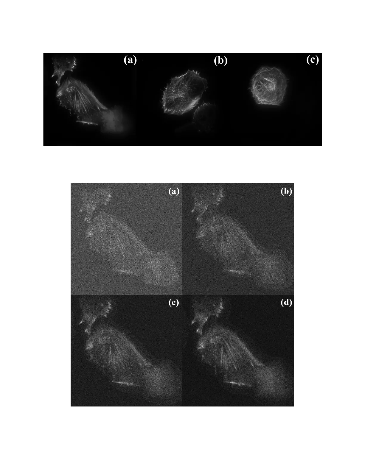
I M A G E R E S T O R A T I O N B Y C O M B I N E D O R D E R R E G U L A R I Z A T I O N W I T H O P T I M A L S PA T I A L A D A P T A T I O N A P R E P R I N T Sanjay V iswanath Imaging Systems Lab Department of Electrical Engineering Indian Institute of Science Bangalore, Karnataka, India 560012 sanjayv@iisc.ac.in Manu Ghulyani Imaging Systems Lab Department of Electrical Engineering Indian Institute of Science Bangalore, Karnataka, India 560012 sanjayv@iisc.ac.in Simon De Beco Laboratoire Physico Chimie Curie Institut Curie 26 rue d’Ulm Paris Cede x 05, France 75248 simondebeco@gmail.com Maxime Dahan* Laboratoire Physico Chimie Curie Institut Curie 26 rue d’Ulm Paris Cede x 05, France 75248 Muthuvel Arigovindan Imaging Systems Lab Department of Electrical Engineering Indian Institute of Science Bangalore, Karnataka, India 560012 mvel@iisc.ac.in *Dedicated to the memory of Maxime Dahan who passed away on 29.07.2018 June 2, 2021 A B S T R AC T T otal V ariation (TV) and related e xtensions hav e been popular in image restoration due to their rob ust performance and wide applicability . While the original formulation is still relev ant after two decades of extensiv e research, its extensions that combine deriv atives of ﬁrst and second orders are no w being explored for better performance, with examples being Combined Order TV (CO TV) and T otal Generalized V ariation (TGV). As an improv ement o ver such multi-order con vex formulations, we propose a nov el non-con ve x regularization functional which adapti vely combines Hessian-Schatten (HS) norm and ﬁrst order TV (TV1) functionals with spatially varying weight. This adaptiv e weight itself is controlled by another regularization term; the total cost becomes the sum of this adapti vely weighted HS-TV1 term, the re gularization term for the adapti ve weight, and the data-ﬁtting term. The reconstruction is obtained by jointly minimizing w .r .t. the required image and the adapti ve weight. W e construct a block coordinate descent method for this minimization with proof of con vergence, which alternates between minimization w .r .t. the required image and the adapti ve weights. W e deri ve exact computational formula for minimization w .r .t. the adaptiv e weight, and construct an ADMM algorithm for minimization w .r .t. to the required image. W e compare the proposed method with existing re gularization methods, and a recently proposed Deep GAN method using image reco very examples including MRI reconstruction and microscopy decon volution. K eywords T otal V ariation, Image Restoration, Multi-Order Re gularization, Hessian-Schatten norm, Spatially Adaptiv e Regularization, Magnetic Resonance Imaging, T otal Internal Reﬂection Fluorescence Microscopy . 0 © 2020 IEEE. Personal use of this material is permitted. Permission from IEEE must be obtained for all other uses, in any current or future media, including reprinting/republishing this material for advertising or promotional purposes, creating new collecti ve works, for resale or redistrib ution to servers or lists, or reuse of any cop yrighted component of this work in other works. A P R E P R I N T - J U N E 2 , 2 0 2 1 1 Introduction Regularization plays an important role in image reconstruction/restoration by stabilizing the in version of the imaging forward model against noise and other distortions in modalities such as photograph y [ 1 ], microscopy [ 2 ], astronomical imaging [ 3 ] and magnetic resonance imaging [ 4 ]. Here we consider the measurement model in which the measured image is expressed as a con volution of the underlying image with a blurring function. In regularized reconstruction, the required image is the solution of the following minimization problem: ˆ s ( r ) = arg min s F ( s, h, m ) + λR ( s ) , (1) where R ( s ) is the regularization functional, and F ( s, h, m ) is the data ﬁdelity term with m being the measured image and h being the blurring kernel of the imaging system. W e restrict the data ﬁdelity term to be of the form, F ( s, h, m ) = X r | ( h ∗ s )( r ) − m ( r ) | 2 (2) Strictly speaking, the data-ﬁdelity term should be the ne gati ve log-lik elihood of the noise model. Howe ver , our focus is on developing improv ed regularization, and hence we use the above form of data-ﬁdelity as an approximation, irrespectiv e of the noise model. In our e valuation of the regularized image reconstruction methods, we consider two types of imaging forward models with respect to our restoration e xperiments. The ﬁrst measurement model is related to total internal reﬂection ﬂuorescence (TIRF) microscopy and is gi ven by m ( r ) = P (( h ∗ s )( r )) + η ( r ) , (3) where h ( r ) is the PSF of TIRF microscope, P ( · ) represents the Poisson process, and η ( r ) is additi ve white Gaussian noise. The second measurement model in volved in our experiments corresponds to magnetic resonance imaging (MRI) and is giv en by ˆ m = T s M F s ( r ) + ˆ η η η , (4) where F represents Fourier transformation operation, M represents the under-sampling mask of ones and zeros, T s represents the operations of picking samples from non-zero locations of M , and ˆ η η η is the complex noise vector where each component comes from a Gaussian distribution. For the ﬁrst case, equation (2) is not the exact negati ve log-likelihood, and for the second case, it is the e xact negati ve log-likelihood. For the MRI model in the second case, h is the in verse Fourier transform of M and m ( r ) = F − 1 ( T † s ˆ m ) , with T † s denoting the adjoint of T s , which is essentially the operation of embedding the Fourier samples into image form. Note that, in this case, m ( r ) can hav e complex v alues and it is taken care by the operator | · | in equation (2). As mentioned before, our focus is on developing an improv ed regularization method. The quality of restoration is mainly determined by the ability of R ( s ) to discriminate between characteristics of the underlying image and noise. While priors can be deﬁned based on general image characteristics such as sparsity of the roughness [ 5 , 6 , 7 , 8 ], there are also priors which are tailored to speciﬁc classes of images [ 9 , 10 , 11 ]. The latter type of regularization approach utilizes learning paradigms including deep learning based techniques [ 12 , 13 , 14 , 15 ], dictionary learning [ 9 , 10 , 16 , 17 ] and model ﬁtting [ 11 ]. Here the functionals are b uilt from training images and then applied for restoration in volving images from the same class. Such methods are believ ed to out-perform general priors, when suitable training sets are av ailable. At the same time, the necessity of training set and computational complexity limits their applicability . On the other hand, general priors such as Tikhono v regularization [ 18 ] and total variation (TV) [ 19 ] do not need training samples and hav e been applied with rob ust performance in multiple domains. Among these general priors, total variation (TV) [ 19 ] has been widely applied [ 5 , 6 , 7 , 8 ] because of its ability to recover sharp image features in the presence of noise and in the cases of undersampling. First order TV (TV1) restoration is giv en by s opt = argmin s F ( s, h, m ) + λ X r k ( d 1 ∗ s )( r ) k 2 | {z } R 1 ( s ) with d 1 ( r ) = [ d x ( r ) , d y ( r )] T , (5) where d x ( r ) and d y ( r ) are ﬁlters implementing ﬁrst order deri vativ es, ∂ ∂ x , and ∂ ∂ y respectiv ely . While TV1 is able to retain edges [ 20 ] in the reconstruction as compared to standard ` 2 norm based T ikhonov regularization [ 18 ], it presents drawbacks such as staircase artifacts [ 21 , 22 ]. Higher order extensions of TV [ 23 , 24 , 25 , 26 ] hav e been proposed to av oid staircase artifacts and they deli ver better restoration, albeit at the cost of increased computations. Second order 2 A P R E P R I N T - J U N E 2 , 2 0 2 1 TV (TV2) [24] restoration was proposed as s opt = argmin s F ( s, h, m ) + λ X r k ( d 2 ∗ s )( r ) k 2 | {z } R 2 ( s ) , with d 2 ( r ) = [ d xx ( r ) d y y ( r ) √ 2 d xy ( r )] T , (6) where d xx ( r ) , d y y ( r ) , and d xy ( r ) are discrete ﬁlters implementing second order deriv atives ∂ 2 ∂ x 2 , ∂ 2 ∂ y 2 and ∂ 2 ∂ x∂ y respectiv ely . Another second-order deriv ativ e based formulation is Hessian-Schatten (HS) norm regularization [ 27 ] [ 26 ], which has been proposed as a generalization of the standard TV2 regularization. It is constructed as an ` p norm of Eigen values of the Hessian matrix, which becomes the standard TV2 for p = 2 . HS norm with p = 1 has been prov en to yield best resolution in the reconstruction, since this better preserves Eigen v alues of the Hessian [ 26 ]. Let H 2 ( r ) be the matrix ﬁlter composed of d xx ( r ) , d y y ( r ) , and d xy ( r ) and let ζ ζ ζ ( · ) be the operator that returns the vector containing the Eigen values of its matrix ar gument. Then HS norm regularization of order p can be expressed as s opt = argmin s F ( s, h, m ) + λ X r k ζ ζ ζ (( H 2 ∗ s )( r )) k p . (7) Since the Eigen values are actually directional second deri v ativ es taken along principle directions, setting p = 1 better preserves the local image structure. It has to be noted that the costs giv en in the equations (5), and (6) are often minimized using gradient based approaches with smooth approximations of the form R k ( s ) = P r p  + || d k ( r ) ∗ s ( r ) || 2 2 , k = 1 , 2 where  is a small positiv e constant [ 19 ], [ 28 ]. This approach has been pro ven to con ver ge to the minimum of the exact form as  → 0 [ 28 ]. Approaches to minimize the cost without smooth approximation include primal-dual method [ 29 ], and alternating direction of multiplier method (ADMM) [ 30 ]. A detailed comparison of such approaches has been provided in [31]. It has been demonstrated that combining ﬁrst- and second-order deriv ati ves is advantageous in accurately restoring image features [32, 33, 34, 35]. In this regard, the combined order TV [33] uses scalar relati ve weights for combining ﬁrst- and second-order v ariations, with the relativ e weights left as user parameters and the solution is estimated by means of optimization problem of the form s opt = argmin s F ( s, h, m ) + λα 1 R 1 ( s ) + λα 2 R 2 ( s ) , (8) where α 1 and α 2 determine the relativ e weights. Although HS norm can be in principle combined with TV1 by the same way as standard TV2 is combined as gi ven abo ve, this possibility has not been explored. A generalization for total v ariation to higher order terms, named as total generalized v ariation (TGV) has also been proposed [ 34 ] [ 36 ]. It is generalized in the following ways: it is formulated for any general deriv ativ e order , and for any given order , it is generalized in the way ho w the deriv ativ es are penalized. In the literature, only the second order TGV form has been well explored for image reconstruction, which takes the follo wing form: ( s opt , p opt ) = argmin s, p F ( s, h, m ) + λα 1 X r k ( d 1 ∗ s )( r ) − p ( r ) k 2 + λα 2 1 2 X r k d 1 ( r ) ∗ p T ( r ) + p ( r ) ∗ d T 1 ( r ) k F , (9) where p ( r ) is an auxiliary 2 × 1 vector image. The TGV functional is able to spatially adapt to the underlying image structure because of the minimization w .r .t. auxiliary variable p . Near edges, p ( r ) approaches zero leading to TV1-like behavior which allo ws sharp jumps in the edges. On the other hand, in smooth regions, p ( r ) approaches d 1 ∗ s ( r ) leading to TV2-like beha vior which will av oid staircase artifacts. Howe ver , the drawback with TGV functional is that the weights α 1 and α 2 hav e to be chosen by the user . In summary , existing combined order methods can bring the advantages of multi-order deri vati ves albeit at the cost of additional tuning. W e propose a novel spatially adapti ve re gularization method, in which, the weights in volved in combining ﬁrst- and second-order deri vati ves are determined from the measured image without user-interv ention. Here the relativ e weight between ﬁrst- and second-order terms becomes an image, and this weight is determined without user -intervention through minimization of a composite cost function. Our contributions can be summarized as follo ws: • W e construct a composite re gularization functional containing two parts: (i) the ﬁrst part is constructed as the sum of ﬁrst- and second-order deri vati ve magnitudes with spatially varying relati ve weights; (ii) the second 3 A P R E P R I N T - J U N E 2 , 2 0 2 1 part is an additional regularization term for pre venting rapid spurious variations in the relati ve weights. For the ﬁrst order term, we use the norm of the gradient, and for the second order term, we use the Schatten norm of the Hessian [ 27 ] [ 26 ]. The composite cost functional is con vex with respect to either the required image or the relativ e weight, b ut it is non-con ve x jointly . • W e construct a block coordinate descent method in volving minimizations w .r .t. the required image and the relativ e weight alternati vely with the following structure: the minimization w .r .t. the required image is carried out using ADMM approach [ 37 , 38 ] and the minimization w .r .t. the relativ e weight is carried out as a single step exact minimization using a formula that we deri ve in this paper . • Since the total cost is non-conv ex, the reconstruction results are highly dependent on the initialization for block-coordinate descent method. W e handle this problem using a multi-resolution approach, where, a series of coarse-to-ﬁne reconstructions are performed by minimization of cost functionals deﬁned through upsampling operators. Here, minimization w .r .t. the relativ e weight and the required image is carried out alternativ ely , as we progress from coarse to ﬁnal resolution le vels. At the ﬁnal resolution le vel, the above-mentioned block coordinate descent method is applied. • Note that the sub-problem of minimization w .r .t. to the required image in volv es spatially v arying relati ve weights. Further , this sub-minimization problem in the above-mentioned multi-resolution loop in volv es upsampling operators. Hence, the ADMM method proposed by Papaﬁtsoros et al. [ 33 ] turns out to be unsuitable. W e propose improv ed variable splitting method and computational formulas to handle this issue. • W e prov e that the overall block coordinate descent method conv erges to a local minimum of the total cost function by using Zangwill’ s conv ergence theorem. This work is an e xtension of the work presented in the conference paper [ 35 ], where we only considered a dif ferentiable approximation of the total v ariation functionals, and did not incorporate the joint optimization of the relati ve weight and the required image. In other words, only the multi-resolution loop is applied without the block-coordinate descent method in the ﬁnal resolution. This method was named Spatially Adaptiv e Multi-order TV (SAM-TV). Here we name the improv ed approach more appropriately as Combined Order Regularization with Optimal Spatial Adaptation (COR OSA). The rest of the paper is organized as follo ws: section 2 deals with the formulation of COROSA functional and the multi-resolution framew ork, and section 3 presents the ADMM formulation and iterations for the optimization problems associated with COR OSA. Section 4 presents the simulation results and comparisons. 2 COR OSA Image Restoration 2.1 COR OSA formulation In the proposed COR OSA approach, the restoration problem is formulated as gi ven belo w: ( s opt , β opt ) = argmin s,β F ( s, h, m ) + λR sa ( s, β , p ) + L ( β , τ ) + B ( s ) , (10) where R sa ( s, β , p ) = X r β ( r ) k ( d 1 ∗ s )( r ) k 2 + X r (1 − β ( r )) k ζ ζ ζ (( H 2 ∗ s )( r )) k p , subject to 0 ≤ β ( r ) ≤ 1 , (11) L ( β , τ ) is a regularization term for β , which will be speciﬁed soon, and B ( · ) is the indicator function for constraining the restored image to a particular range of positive v alues. From this formulation, it is clear that the relati ve weight image β is also considered as a minimization v ariable and the optimal image of weights is determined jointly with the required image. Since R sa ( s, β , p ) is linear in β , minimizing with respect to β means that it will essentially act as a switching between ﬁrst- and second-order terms. In this context, the role of L ( β , τ ) is to prev ent spurious switching; in other words, its role is to prevent rapid switching between the ﬁrst- and second-order terms caused by insigniﬁcant differences in their magnitudes. W e set L ( β , τ ) as L ( β , τ ) = − X r τ log( β ( r )(1 − β ( r ))) . (12) Here, a lo wer value of τ will cause a more rapid switching between ﬁrst- and second-order terms and vice versa. W e denote the ov erall cost by J sa ( s, β , τ , h, m ) , and we write J sa ( s, β , τ , h, m ) = F ( s, h, m ) + λR sa ( s, β , p ) + L ( β , τ ) + B ( s ) . (13) 4 A P R E P R I N T - J U N E 2 , 2 0 2 1 An assumption that is implicitly made by most of the image restoration algorithms is that there is no s for which F ( s, h, m ) , R 1 ( s ) = P r k ( d 1 ∗ s )( r ) k 2 , and R 2 ( s ) = P r k ( H 2 ∗ s )( r ) k 2 will hav e zero val ue simultaneously . W e will also use this assumption for proving the conv ergence of the iterati ve method that we propose in the follo wing sections. 2.2 Multiresolution method The regularization functional, R sa ( s, β , p ) , is non-con ve x jointly with respect to β and s , although it is con ve x with any one of them alone. Hence, the reconstruction result becomes sensiti ve to initialization and ﬁnding an ef ﬁcient initialization becomes crucial. T o this end, we adopt multiresolution approach for the initialization. T o describe the multi-resolution approach, we deﬁne the following: F ( j ) ( s, h, m ) = X r | ( h ∗ ( E ( j ) s ))( r ) − m ( r ) | 2 . (14) R ( j ) sa ( s, β , p ) = X r β ( r ) k ( d 1 ∗ ( E ( j ) s ))( r ) k 2 X r (1 − β ( r ))    ζ ζ ζ (( H 2 ∗ ( E ( j ) s ))( r ))    p . (15) In the above, E ( j ) s denotes the image obtained by interpolating s by a factor 2 j along both axes. W e will defer the description of the implementation of E ( j ) to the end. Here, ( h ∗ ( E ( j ) s ))( r ) denotes con volving the interpolated image E ( j ) s with h followed by accessing the pix el at position r . Further , ( d 1 ∗ ( E ( j ) s ))( r ) and ( H 2 ∗ ( E ( j ) s ))( r )) hav e similar interpretation except that the ﬁrst expression will be a vector , and the second one will be a matrix. Note that the variable s is an N 2 j × N 2 j image in both the functionals F ( j ) ( s, h, m ) , and R ( j ) sa ( s, β , τ , p ) . On the other hand, β always has size N × N , which is the size of the measurement m ( r ) . W e denote the resulting scale- j cost by J ( j ) sa ( s, β , τ , h, m ) = F ( j ) ( s, h, m ) + λR ( j ) sa ( s, β , p ) + L ( β , τ ) + B ( E ( j ) s ) . (16) It should be noted that, size of the v ariable in scale- j cost is N 2 j × N 2 j ; ho wev er , the cost is al ways e valuated on a N × N grid through interpolation by E ( j ) . This will help to ensure a better con ver gence in the multi-resolution method to be described below . Let K denote the user -deﬁned number of multi-resolution lev els. T o initialize the multi-resolution loop, we set β ( r ) = 0 and perform the following minimization: ˆ s ( K ) ( r ) = argmin s J ( K ) sa ( s, β , τ , h, m ) ≡ argmin s F ( K ) ( s, h, m ) + λR ( K ) sa ( s, β , p ) + B ( E ( K ) s ) . (17) W ith ˆ s ( K ) as the initialization, we iterate for j = K − 1 , . . . , 0 with the follo wing minimizations: f = E ( j +1) ˆ s ( j +1) ¯ β ( r ) = argmin β J sa ( f , β , τ , h, m ) ≡ argmin β R sa ( f , β , p ) + L ( β , τ ) , (18) subject to 0 ≤ β ( r ) ≤ 1 . ˆ s ( j ) ( r ) = argmin s J ( j ) sa ( s, ¯ β , τ , h, m ) ≡ argmin s F ( j ) ( s, h, m ) + λR ( j ) sa ( s, ¯ β , p ) + B ( E ( j ) s ) . (19) The resulting restored image at the end of the multi-resolution loop, ˆ s (0) , can be an initialization for the joint minimization problem giv en in equation (10) . Note that, the minimization problem of equation (19) has to be done iterativ ely and requires an initialization. W e use E (1) ˆ s ( j +1) ( r ) as the initialization. In this regards, the way the multi-scale costs { J ( j ) sa ( s, β , τ , h, m ) , j = 0 , . . . , K } are constructed signiﬁcantly helps to make the initialization E (1) ˆ s ( j +1) ( r ) to be very close the the required minimum ˆ s ( j ) ( r ) . In other w ords, since each J ( j ) sa is constructed through 2 j -fold interpolation on the original reconstruction grid, the initialization E (1) ˆ s ( j +1) ( r ) is typically very close the the required minimum ˆ s ( j ) ( r ) . 5 A P R E P R I N T - J U N E 2 , 2 0 2 1 In the multi-resolution method described above, if we set p = 2 , the result ˆ s (0) will be equiv alent to ﬁnal reconstruction of SAM-TV approach [ 35 ] except the fact that SAM-TV uses smooth approximations for the ﬁrst- and second-order TV terms, whereas, here, the exact non-dif ferentiable form of TV functionals are used. Now we consider solving the sub-problem of determining the adapti ve weight ¯ β in equation (18) . The exact solution for ¯ β is gi ven in the follo wing Proposition. Proposition 1. Let d ( r ) be deﬁned as d ( r ) = k ( d 1 ∗ f )( r ) k 2 − k ζ ζ ζ (( H 2 ∗ f )( r )) k p . (20) If d ( r ) = 0 , the solution for the pr oblem in equation (18) is ¯ β ( r ) = 0 . 5 . When d ( r ) is non-zer o, the solution ¯ β is unique and given by ¯ β ( r ) = 1 2 1 − sig n ( d ( r )) s 4 τ 2 d 2 ( r ) + 1 − 2 τ | d ( r ) | !! . (21) The proof of Proposition 1 is gi ven in Appendix. Next, unlike equation (18) , the subproblem of equation (19) cannot be solved e xactly and has to be solved iterati vely . W e will dev elop an ADMM based method to solve this problem in Section 3. Now it remains to specify the implementation of E ( j ) . It can be implemented by j stages of 2 -fold interpolation. The 2 -fold interpolation can be implemented by inserting a zero next to each pixel along both axes (which is called as the two-fold expansion) and then ﬁltering by an appropriate interpolation ﬁlter . In our implementation we use u ( r ) = 1 64 [1 4 6 4 1] T [1 4 6 4 1] as the interpolation ﬁlter , which is the two-scale ﬁlter of cubic B-spline [39]. 2.3 Obtaining the ﬁnal restoration by block coordinate descent method By using the result of the abo ve multiresolution method as the initialization, the ﬁnal reconstruction has to be obtained by minimizing the cost of equation (10) jointly with respect to β and s . W e propose to use a simple block coordinate descent method. Let s (0) = ˆ s (0) , where ˆ s (0) is the result of the multi-resolution loop described before. W ith k = 0 , . . . , N b , the block coordinate descent method in v olves the follo wing series of minimizations with respect to β and s . Let s ( k ) and β ( k ) be the current estimate of the minimum at c ycle k . Then the next reﬁned estimate is computed as the follo wing set of minimizations: β ( k +1) = argmin β J sa ( s ( k ) , β , τ , h, m ) = argmin β R sa ( s ( k ) , β , p ) + L ( β , τ ) . (22) s ( k +1) = argmin s J sa ( s, β ( k +1) , τ , h, m ) = argmin s F ( s, m, h ) + λR sa ( s, β ( k +1) , p ) + B ( s ) . (23) As evident, the iterations giv en above are similar to the iterations giv en in the multi-resolution method of section 2.2. The difference is that the minimization with respect to β and s for each of the cost functions in the series { J ( j ) sa ( s, β , τ , h, m ) , j = 0 , . . . , K } is done only once in the multiresolution method. On the other hand, the minimiza- tions in the block coordinate decent method (BCD) represented by the equation (22) and (23) are done alternativ ely on the same cost function J sa ( s, β , τ , h, m ) until con ver gence. The functional J sa ( s, β , τ , h, m ) is con ve x with respect to either of s and β , and the BCD method represented by equations (22) and (23) con ver ges to the solution of the problem giv en in (10), provided that each of the minimizations is e xact as per the con ver gence theorem of Bertsekas [40]. Now we consider solving the sub-problems. The subproblems of determining the adaptive weight ¯ β in the block coordinate descent method of equation (22) is identical to the sub-problem of the multi-resolution method (equation (18) ), and hence can be solved e xactly . On the other hand, the sub-problem of equation (23) is similar to the problem of the equation (19) , and cannot be solved exactly . Hence the conv ergence result of Bertsekas [ 40 ] will not be applicable. Howe ver , it is easy to sho w that BCD iteration con ver ges to the minimum if J sa ( s ( k +1) , β ( k +1) , τ , h, m ) < J sa ( s ( k ) , β ( k +1) , τ , h, m ) using Zangwill’ s global con ver gence theorem. W e will provide the con vergence statement along with the proof after describing the ADMM method for solving the problems of equations (19) and (23) in the next section. 6 A P R E P R I N T - J U N E 2 , 2 0 2 1 3 Image reco very with ﬁxed r elative weight f or ﬁrst- and second-order derivativ es The main computational task in the block coordinate descent iteration represented by the equations (22) and (23) , is the computation of s ( k +1) . Similarly , in the multi-resolution method represented by equations (18) and (19) , the main task is the computation of ˆ s ( j ) ( r ) . Note that the cost in (19) becomes algebraically identical to the cost of (23) for j = 0 . Hence the cost in equation (23) can be considered as a special case of the cost in the equation (19) . So we consider only the description of the minimization of the cost in (19) . W e will use the ADMM approach for solving the minimization problem gi ven in the equation (19) . Here, the result of pre vious le vel j + 1 , denoted by ˆ s ( j +1) , can be used for initializing after interpolating by f actor of tw o. Although ADMM is well-kno wn and its application for total v ariation based image restoration is not ne w [ 30 , 41 , 42 , 43 ], implementation of standard ADMM causes some numerical problems because of the spatially varying relati ve weight ¯ β . In the follo wing, we will ﬁrst describe the formulation that will lead to standard ADMM and then describe the modiﬁcation necessary to handle the associated numerical issues. The ﬁrst step in constructing an ADMM algorithm for minimizing composite functionals is to deﬁne an equiv alent constrained optimization such that the sub-functionals act on dif ferent set of variables that are related by means of linear equality constraints. Then writing the augmented Lagrangian [ 40 ] for the constrained problems leads to the required ADMM algorithm. 3.1 Constrained formulation and v ariable splitting For notational con venience, we switch to vector based notations. Let the N × N image s ( r ) be represented by scanned vector s in R N 2 , such that its i th element s i is giv en by s i ( r 0 ) = s ( r 0 ) with r 0 = [ r 1 r 2 ] satisfying i ( r 0 ) = r 2 N + r 1 . Let m and ¯ β β β also be deﬁned from m ( r ) and ¯ β ( r ) in a similar way with the components denoted by m i and ¯ β i . Let H be the matrix equi valent of con volving an image with h ( r ) , such that the scanned vector of ( h ∗ s )( r ) is gi ven by Hs . Next, let E ( j ) be the matrix equiv alent of interpolation by a factor 2 i . W ith this, the scanned vector of E ( j ) s ( r ) is giv en by E ( j ) s . In terms of the new notational scheme, the data ﬁdelity term can be written as F ( j ) ( s , H , m ) =    HE ( j ) s − m    2 2 . (24) Similarly , let D x , D y , D xx , D y y , and D xy be the matrices deﬁned from d x ( r ) , d y ( r ) , d xx ( r ) , d y y ( r ) , and d xy ( r ) for representing con v olution operations. Let D f = [ D T x D T y ] T and let D s = [ D T xx D T y y D T xy ] T . Let S ( v ) : R 3 → R 4 be the mapping that returns  v 1 v 3 v 3 v 2  , where v = { v 1 , v 2 , v 3 } ∈ R 3 represents the three second order deriv atives. Let P i be a 2 × 2 N 2 matrix having ones at locations (1 , i ) , and (2 , N 2 + i ) and zeros at all other locations. Let Q i be the 3 × 3 N 2 matrix having ones at locations (1 , i ) , (2 , N 2 + i ) , and (3 , 2 N 2 + i ) and zero at other locations. Then we can use the following substitutions in Eq.(15): k ( d 1 ∗ ( E ( j ) s ))( r ) k 2 =    P i ( r ) D f E ( j ) s    2 (25)    ζ ζ ζ (( H 2 ∗ ( E ( j ) s ))( r ))    p =    ζ ζ ζ ( S ( Q i ( r ) D s E ( j ) s ))    p (26) W ith these, the regularization functional can be e xpressed as R ( j ) sa ( s , β β β , p ) = N 2 X i =1 ¯ β i    P i D f E ( j ) s    2 + N 2 X i =1 (1 − ¯ β i )    ζ ζ ζ ( S ( Q i D s E ( j ) s ))    p , (27) where we hav e replaced the images s and ¯ β by the components of their vectorial form. Next, to simplify the task of expressing and comparing the two forms of ADMM, we introduce tw o more deﬁnitions as gi ven belo w: N f ( u , v ) = N 2 X i =1 u i k P i v k 2 (28) N s ( u , w , p ) = N 2 X i =1 u i k ζ ζ ζ ( S ( Q i w )) k p (29) Note that u ∈ R N 2 , v ∈ R 2 N 2 , and w ∈ R 3 N 2 . W ith these, the regularization can be e xpressed as λR ( j ) sa ( s , β β β , p ) = N f ( λ β β β , D f E ( j ) s ) + N s ( λ ( 1 − β β β ) , D s E ( j ) s , p ) (30) 7 A P R E P R I N T - J U N E 2 , 2 0 2 1 where 1 is the v ector of ones. No w the minimization of F ( j ) ( s , H , m ) + λR ( j ) sa ( s , β β β , p ) + B ( E ( j ) s ) can be equi valently expressed as ( s ∗ , d ∗ f , d ∗ s , d ∗ 0 ) = argmin s , d f , d s , d 0 F ( j ) ( s , H , m ) + N f ( λ β β β , d f ) + N s ( λ ( 1 − β β β ) , d s , p ) + B ( d 0 ) , (31) subject to the conditions that D f E ( j ) s = d f , D s E ( j ) s = d s , E ( j ) s = d 0 . (32) This constrained formulation of the reconstruction problem leads to the ADMM algorithm, which is essentially a series of cyclic minimization of individual sub-functionals of the abov e cost. Howe ver , through some reconstruction trials, we found that ADMM method obtained from this formulation lea ves some artifacts in the reconstruction. These artifact disappear only with very lar ge number of iterations. Here we present an alternati ve formulation that leads to a better con ver ging ADMM algorithm. T o this end, we ﬁrst recognize that the cost giv en in the equation (30) can also be expressed as λR ( j ) ec ( s , β β β , p ) = N f ( λ 1 , D 0 f E ( j ) s ) + N s ( λ 1 , D 0 s E ( j ) s , p ) (33) where D 0 f = [ D T x B D T y B ] T (34) D 0 s = [ D T xx ( I − B ) D T y y ( I − B ) D T xy ( I − B )] T (35) with B = diag ( β β β ) . The corresponding constrained problem becomes ( s ∗ , d ∗ f , d ∗ f , d ∗ 0 ) = argmin s , d f , d f , d 0 F ( j ) ( s , H , m ) + N f ( λ 1 , d f ) + N s ( λ 1 , d s , p ) + B ( d 0 ) , (36) subject to condition that D 0 f E ( j ) s = d f , D 0 s E ( j ) s = d s , E ( j ) s = d 0 . (37) From our experiments, we found that the ADMM steps constructed based on the abo ve constrained formulation leads to better con ver ging algorithm. 3.2 A ugmented Lagrangian and the ADMM steps Writing the ADMM steps for the abo ve problem is straightforw ard and well-known in the literature. Howe ver , for proving the con ver gence of block coordinate descent method represented by equations (22) and (23) , we need to specify the steps here. Further , the constraint of the modiﬁed formulation gi ven by equation (37) in v olves non-circulant matrices and hence, it requires some special consideration. T o proceed further , we use the symbol ¯ s in the place of s to av oid notational conﬂict with the iterations of equations (18) and (19) . T o construct the ADMM algorithm from the abov e constraint form of the problem, we deﬁne C ( ¯ s , d f , d s , d 0 , w ) = γ 2     D 0 f E ( j ) ¯ s − d f    2 2 +    D 0 s E ( j ) ¯ s − d s    2 2 +    E ( j ) ¯ s − d 0    2 2  + w T     D 0 f D 0 s I   E ( j ) ¯ s − " d f d s d 0 #   (38) where w represents Lagrangian multipliers [40]. Let J a ( ¯ s , d f , d s , d 0 , λ ) = F ( j ) ( ¯ s , H , m ) + N f ( λ 1 1 1 , d f ) + N s ( λ 1 1 1 , d s , p ) + B ( d 0 ) , (39) and L a ( ¯ s , d f , d s , d 0 , w , λ ) = J a ( ¯ s , d f , d f , d 0 , λ ) + C ( ¯ s , d f , d s , d 0 , w ) (40) Let ¯ s ( j ) be the vector of length N 2 / 2 2 j obtained by scanning E (1) ˆ s ( j +1) ( r ) , where ˆ s ( j +1) ( r ) is the result of pre vious iteration in the multi-resolution loop of the equations (18) and (19) . Then ADMM iterations proceed as follo ws for 8 A P R E P R I N T - J U N E 2 , 2 0 2 1 k = 0 , 1 , 2 , . . . : d ( k +1) f = argmin d f L a ( ¯ s ( k ) , d f , d ( k ) s , d ( k ) 0 , w ( k ) , λ ) (41) d ( k +1) s = argmin d s L a ( ¯ s ( k ) , d ( k +1) f , d s , d ( k ) 0 , w ( k ) , λ ) (42) d ( k +1) 0 = argmin d 0 L a ( ¯ s ( k ) , d ( k +1) f , d ( k +1) s , d 0 , w ( k ) , λ ) (43) ¯ s ( k +1) = argmin ¯ s L a ( ¯ s , d ( k +1) f , d ( k +1) s , d ( k +1) 0 , w ( k ) , λ ) (44) w ( k +1) = w ( k ) + γ      D 0 f D 0 s I   E ( j ) ¯ s ( k +1) −    d ( k +1) f d ( k +1) s d ( k +1) 0       (45) W e will use the partitioned notation w ( k ) =    w ( k ) f w ( k ) s w ( k ) 0    for deﬁning the solution for the abov e minimization problems. First note that L a ( ¯ s , d f , d s , d 0 , w , λ ) is non-differentiable w .r .t. d f , d s , and d 0 , and we use the notion of proximal map to carry out the minimization deﬁned in the equations (41), (42), and (43). The minimization w .r .t. d f giv en in the equation (41) is essentially the minimization of γ 2    D 0 f E ( j ) ¯ s − d f    2 2 + ( w ( k ) f ) T ( D 0 f E ( j ) ¯ s − d f ) + N f ( λ 1 1 1 , d f ) , w .r .t. d f . This can be rewritten as γ 2    ¯ d ( k ) f − d f    2 2 + N f ( λ 1 1 1 , d f ) + const. , where ¯ d ( k ) f = D 0 f E ( j ) ¯ s ( k ) + (1 /γ ) w ( k ) f , and const is a term that is independent of d f . The minimum of this cost is deﬁned as the proximal map of N f ( λ 1 1 1 , · ) applied on ¯ d ( k ) f [44]. This map is expressed as [44] d ( k +1) f = N 2 X i P T i T ( P i ¯ d ( k ) f , λ/γ ) , (46) where T ( x , t ) denotes the soft-threshold operator given by T ( x , t ) = max (0 , k x k 2 − t ) x k x k 2 . (47) Similarly , solution to the minimization problem giv en in equation (42) is the proximal map of N s ( λ 1 , · , p ) applied on ¯ d ( k ) s = D 0 s E ( j ) ¯ s ( k ) + (1 /γ ) w ( k ) s . Let ||| · ||| t denote the operator that applies soft-thresholding on the Eigen v alues of its matrix arguments and returns the resulting matrix. Then the proximal map of N s ( λ 1 , · , p ) can be expressed as [ 26 ] d ( k +1) s = N 2 X i Q T i H T ( Q i ¯ d ( k ) s , λ/γ , p ) , (48) where H T ( x , t, p ) = ( max ( kS ( x ) k F − t, 0) x kS ( x ) k F , for p = 2 S − 1 ( |||S ( x ) ||| t ) , for p = 1 (49) Finally , the minimum deﬁned in equation (43) is the proximal map of B ( d 0 ) applied on ¯ d ( k ) 0 = E ( j ) ¯ s ( k ) + (1 /γ ) w ( k ) 0 . This is denoted as d ( k +1) 0 = P u ( ¯ d ( k ) 0 ) , where P u ( · ) denotes the clipping of components of the its vectors onto the range [0 , b ] , with b as the user-deﬁned upper bound. The cost L a ( ¯ s , d f , d s , d 0 , w , λ ) is differentiable w .r .t. ¯ s , and the minimization deﬁned in the equation can be obtained by equating gradient to zero. Let M =   D 0 f D 0 s I   and let d ( k +1) =    d ( k +1) f d ( k +1) s d ( k +1) 0    . Then, the solution of the last minimization is giv en by the follo wing equation, E ( j ) T M T ME ( j ) | {z } A j s ( k +1) = v k +1 , (50) 9 A P R E P R I N T - J U N E 2 , 2 0 2 1 where v k +1 = E ( j ) T M T  d ( k +1) − (1 /γ ) w ( k +1)  . Note that this equation has to be solved iterati vely since M is composed of non-circulant matrices. W e use conjugate gradient method for solving this problem. T o speed-up, we use the in verse of the follo wing approximation of the matrix A j in the equation (50), ˆ A j , as the preconditioner: ˆ A j = E ( j ) T  D T f D f + D T s D s + I  E ( j ) (51) All the matrices in the abov e product are circulant e xcept E ( j ) . Howe ver , the product, ˆ A j , is circulant because of the special structure of E ( j ) . Hence, the preconditioning, i.e., multiplying by the in verse of ˆ A j , is equi valent to applying the in verse of a discrete ﬁlter . The following proposition gi ves the expression for this ﬁlter . Proposition 2. Let u ( z 1 , z 2 ) be the z-transform of u ( r ) = 1 64 [1 4 6 4 1] T [1 4 6 4 1] , and let u j ( z 1 , z 2 ) = Q j − 1 i =0 u ( z 2 i 1 , z 2 i 2 ) . Let u j ( r ) be the in verse z-transform of u j ( z 1 , z 2 ) . Then the ﬁlter equivalent of ˆ A j is the 2 j -fold decimation of B ( r ) = u j ( r ) ∗ u j ( − r ) ∗ [1 + d x ( r ) ∗ d x ( − r ) + d y ( r ) ∗ d y ( − r ) + d xx ( r ) ∗ d xx ( − r ) + d y y ( r ) ∗ d y y ( − r ) + d xy ( r ) ∗ d xy ( − r )] . Next, applying these ADMM steps described abo ve for solving the minimization problem of equation (23) is nearly identical except the fact that the up-sampling matrix E is replaced by identity matrix because the cost is not deﬁned through up-sampling. Here the size of the v ariable is the same as the size of the measured image. The initialization for ADMM iteration, ¯ s (0) , no w simply comes from s ( k ) , which is the result of pre vious iteration of the BCD loop represented by equations (22) and (23) . Next, the follo wing proposition conﬁrms the con ver gence of the block coordinate descent algorithm speciﬁed by the equations (22) and (23). Proposition 3. The bloc k coor dinate descent method repr esented by the equations (22) and (23) with the pr oblem of equation (23) solved by ADMM method described above, con ver ges to a local solution of the pr oblem (10) if J sa ( s ( k +1) , β ( k +1) , τ , h, m ) < J sa ( s ( k ) , β ( k +1) , τ , h, m ) and if there is no s for whic h F ( s, h, m ) , R 1 ( s ) = P r k ( d 1 ∗ s )( r ) k 2 , and R 2 ( s ) = P r k ( H 2 ∗ s )( r ) k 2 will have zer o value simultaneously . 4 Experimental results For e v aluating the restoration performance of the proposed COR OSA approach, we considered deconv olution of T otal Internal Reﬂection Fluorescence (TIRF) microscopy images and the reconstruction of Magnetic Resonance Images (MRI) from under-sampled F ourier data. These problems in volve dif ferent measurement and noise models and are hence good candidates for e valuating the performance of the proposed approach alongside the state-of-the-art methods. W e compare COR OSA with second order TV (TV2) [ 24 ], Hessian-Schatten norm regularization (HS) [ 26 ], combined order TV (CO TV) [ 33 ] and TGV2 [ 36 ] regularization methods. W e also implemented the combined order TV formulation with Hessian-Schatten norm regularization replacing the original second order TV term, for the purpose of comparison. W e refer to this method as Combined Order Hessian-Schatten (COHS) regularization. For the HS functional, we found that setting p = 1 yielded the best performance. W e also include the result of the multi-resolution loop represented by equations (18) and (19) in the comparison (without BCD iterations of equations (22) and (23) ). W e denote this by COR OSA-I. F or objecti ve comparison, we use Signal to Noise Ratio (SNR) [ 45 ] and Structural Similarity Index (SSIM) [46] scores. In tables, we use COR. and COR-I to denote COR OSA and COR OSA-I respecti vely . The smoothing parameter λ was tuned for best performance in terms of SSIM and SNR by using original reference images as done by most methods that focus on the design of regularization. In the case of CO TV , and COHS, additional tuning is required to ﬁx the parameters determining the ﬁrst and second order TV terms. In this regard, we set the relativ e weights between ﬁrst and second order deriv ativ es so as to yield the lowest regularization functional cost. This ensures that only λ is required to be tuned using the reference images. The spatial weight β ( r ) can be determined through optimization problem deﬁned in (18) and the corresponding result is given in Proposition 1, with the parameter τ chosen to be a scalar parameter . Howev er , we observed that it is adv antageous to make τ spatially variant for the follo wing reasons: (i) in the re gions of low intensity , it is advantageous to make β ( r ) less sensiti ve to v ariations in the rel ativ e magnitude of ﬁrst- and second-order deriv atives, and hence τ has to be larger; (ii) in the regions of high intensity , it is advantageous to mak e β ( r ) more sensitiv e to variations in the relati ve magnitude of these terms, and hence τ has to be smaller . In short, it is adv antageous to mak e τ spatially variant and in versely proportional to some approximate estimate of the required image, say ¯ f ( r ) . W e use the following strate gy to get this approximate estimate: (i) for solving the problem giv en the equation (18) , we use f itself as the approximate estimate, i.e., we set ¯ f ( r ) = f ( r ) . Next, in the block-coordinate descent loop speciﬁed by the equations (22) and (23) , we keep ¯ f ( r ) ﬁxed as the image used to initialize the loop, that is we set ¯ f ( r ) = s (0) ( r ) . From ¯ f ( r ) , we compute τ ( r ) as follows: we compute the image exp( − 100 ∗ ¯ f 2 ( r )) and then rescale it to the range [0 . 01 , 100] . This scheme w orked well for all our test cases, and hence we kept this scheme for determining τ ( r ) in all test cases. 10 A P R E P R I N T - J U N E 2 , 2 0 2 1 Figure 1: TIRF model images: (a) ActinSample1; (b) ActinSample2; (c) Tub ulinSample. Figure 2: Blurred noisy images obtained from ActinSample1: (a) γ p = 5 ; (b) γ p = 10 ; (c) γ p = 20 ; (d) γ p = 30 . 11 A P R E P R I N T - J U N E 2 , 2 0 2 1 In the ﬁrst experiment, we ev aluate the proposed method for deconv olution of TIRF images. T o obtain realistic ground-truth models, we measured TIRF images with negligible noise and decon volv ed them by a simple inv erse ﬁltering. The resulting images became the ground truth models, which were used to simulate noisy blurred images for e valuating the proposed method and for comparing it with the e xisting methods. The images for generating ground-truth model were acquired from samples containing labelled Actin and T ubulin. The Actin images were acquired by staining with phalloidin-488 and an EMTB-mCherry transgene was used to get the T ubulin image. W av elength for excitation was 491nm for Actin samples and 561nm for T ubulin sample. All images were acquired using a 100x objecti ve lens with numerical aperture 1.45 N A. The exposure time was set to 300ms, and this was suf ﬁcient to get nearly noise-free images with a quality that is adequate for using them as ground-truth models. These are shown in Figure 1. For simulating noisy blurred images from ground-truth models, we used blurring kernel with a bandwidth that is slightly lower than the bandwidth of the system that measured the model images. This was done by setting N A = 1.4, while computing the required blurring kernel. W e used the following model to generate test images: m ( r ) = P [ γ p ( h ∗ s )( r ))] + η ( r ) (52) Here h ( r ) represents the simulated 2D TIRF PSF with N A = 1.4, and with other parameters set to be identical to that of the system that measured the models. Next, P ( · ) refers to Poisson process with γ p representing the scale factor for photon count, and η is A WGN of variance σ η . W e use this mixed noise model to make the test data realistic, although we do not use the log-likelihood functional of the mix ed model in the formulation of our method. For each reference model, we set σ η = 1 and generated four noisy blurred images with γ p = 5, 10, 20, and 30. The four noisy images corresponding to ActinSample1 are sho wn in Figure 2 as an e xample. It has to be pointed out that we did not include TGV in this e xperiment because of its poor performance, as w as observed in [ 35 ]. In this regard, it is worthwhile to note that TGV has been used notably only for MRI reconstruction. The decon volution r esults in terms of both SSIM and SNR scores are presented in T able 1. The scores show that the proposed COR OSA outperforms other methods in most cases, with the performance advantage signiﬁcant when the noise is high. It is to be noted that TV2 gi ves slightly better scores than COR OSA as the measurements become less noisy . This is due to the fact that the ef fect of spatial adapti veness is ne gligible, and the f act that, TV2 can con verge to the minimum more accurately because of its simplicity , which takes ov er the advantage of spatial adapti veness. Ho wev er , in such lo w-noise cases, the difference in the score is much lo wer than the adv antage that COR OSA has in noisy cases. Figure 3 sho ws a set of restored images corresponding to ActinSample1 image and γ p = 20 . In terms of SSIM, the dif ference between TV2 and COR OSA is 0.006 and difference in SNR is 0.2dB. Ho we ver , as evident from the displayed images, there is a clear visual improvement in the result of COR OSA. Another observation is that COR OSA signiﬁcantly outperforms CO TV and COHS, because of the spatial adaptivity . T able 1: Comparison of decon volution results for TIRF images IMG γ p SSIM SNR TV2 HS CO TV COHS COR-I COR. TV2 HS CO TV COHS COR-I COR. Act.1 5 .725 .731 .502 .502 .728 .762 10.53 10.58 9.37 9.37 10.58 10.97 10 .794 .793 .679 .679 .792 .807 13.44 13.45 12.88 12.89 13.40 13.82 20 .853 .849 .806 .807 .848 .853 15.62 15.64 15.38 15.43 15.59 15.90 30 .890 .888 .867 .867 .887 .890 16.88 16.91 16.81 16.81 16.81 17.08 Act.2 5 .735 .744 .516 .516 .741 .780 12.03 12.06 10.74 10.74 12.05 12.34 10 .828 .829 .712 .712 .829 .844 14.59 14.58 13.96 13.97 14.58 14.74 20 .883 .881 .839 .839 .880 .882 16.58 16.56 16.38 16.39 16.54 16.55 30 .904 .900 .880 .880 .897 .899 17.69 17.66 17.58 17.59 17.60 17.57 T ub .1 5 .769 .784 .491 .491 .780 .827 13.42 13.60 11.30 11.30 13.57 13.92 10 .830 .832 .685 .685 .830 .844 15.70 15.71 14.76 14.76 15.69 15.86 20 .868 .864 .806 .806 .863 .862 17.46 17.52 17.17 17.18 17.50 17.55 30 .881 .877 .850 .850 .875 .875 18.27 18.29 18.07 18.11 18.23 18.25 In the second experiment, we considered reconstruction of MRI images from undersampled k-space measurements. The source MRI images are sho wn in Figure 4. It has to be mentioned that some of these reference images have been obtained using traditional reconstruction methods and hence contain artifacts. Howe ver , this does not affect the validity of our comparisons done here, because, all the methods ev aluated in this paper including the proposed method remove these artifacts. Hence, we focus on ho w well the actual structures are reproduced by v arious methods in the presence of noise and undersampling, and ignore the remo val of artif acts present in the reference images. For sampling, we generated random and spiral trajectories using the MA TLAB code given by Chauf fert et al. [ 47 ]. In addition, we modiﬁed the spiral trajectory by ﬁlling in lo w frequency re gion, since the default spiral had lo w sample density in the 12 A P R E P R I N T - J U N E 2 , 2 0 2 1 Figure 3: ActinSample1 Restoration: (a) Original Image; (b) Blurred Noisy Image with γ p = 20 ; (c) TV2; (d) HS; (e) CO TV ; (f) COHS; (g) COROSA-I; (h) COR OSA. 13 A P R E P R I N T - J U N E 2 , 2 0 2 1 Figure 4: MRI Reference Images Figure 5: MRI T rajectories. Random: (a) 10% (b) 20%, Spiral: (c) 10% (d) 20% low frequency re gion. Both sampling trajectories with 10% and 20 % densities are shown in Figure 5. For simulating the thermal noise, we added white Gaussian noise to the k-space data. T o control the noise, we use the strate gy of [ 10 ]: the Gaussian v ariance is adjusted such that, if added to both real and imaginary parts of full F ourier transforms of the image, it results in PSNR of 10dB and 20dB upon the Fourier in version. W e generated six sample sets from each MRI image as follo ws: for each sampling trajectory , we generated 20% sample set with two noise lev els (10dB and 20dB), and 10% sample set with one noise lev el (20dB). This make a total of 36 sample sets. The comparisons in terms of SSIM and SNR scores for all cases are giv en in T able 2. The reconstruction scores in T able 2 show that, in most cases, the proposed COROSA approach is better than all competitiv e methods, with CO TV and COHS being the nearest in terms of scores. In terms of SSIM, COR OSA is always better, and in terms of SNR, COR OSA is better in most of the cases. In general, combined order methods perform better in MRI reconstruction, when compared to TIRF restoration. Figure 6 sho ws the reconstruction results for MRI 6 image with 10% sampling and 20dB PSNR samples. It is clear from the ﬁgure that COR OSA suppresses background artif acts with the help of spatial adaptation better than TV2 and HS. At the same time, COR OSA also a v oids staircase artifacts that is normally caused if TV1 is used without spatial adaptation as present in CO TV and COHS reconstructions. A selected region of this reconstruction is shown in Figure 7 to further emphasize this fact, along with the relativ e weight β ( r ) . In the ﬁgure, white regions correspond to locations where ﬁrst order TV term is dominant, and black regions correspond to locations where second order TV term is dominant. Grey regions represent locations where both orders are weighted equally . It is clear from the ﬁgure that spatial weights follow the local intensity structure, leading to the elimination of staircase artifacts. On the other hand, such artif acts are e vident in CO TV reconstruction, which uses similar cost function and optimization framew ork, albeit with constant global relativ e weights. Recall that SSIM of COR OSA for this selected re gion is 0.7663 and that of CO TV is 0.7324. Figure 8 shows the e volution of adaptiv e weight β ( r ) across different stages of multi-resolution and block coordinate descent iterations. It can be noted that β ( r ) follows ﬁne v ariations in the relati ve magnitudes of ﬁrst- and second-order deri v ativ es that are not ob vious from the visual inspection of the displayed intensity images. W e have also gi ven the reconstruction results for MRI 1 image with 10% sampling and 20dB PSNR samples in Figure 9, conﬁrming that the visual improvement with COR OSA is consistent with the higher scores. Further, CO TV and COHS introduce prominent artifacts in the reconstruction as seen in zoomed-in view of the same set of images displayed in Figure 10 along with β ( r ) . It is also clear that these artifacts are not the remnants of any artifacts from the original model, but were produced by CO TV and COHS methods. On the other hand, COR OSA results do not ha ve any artif acts and the adaptiv e weights clearly pick out image boundaries from uniform intensity regions. There are two e xceptions in the results that do not confer to the pattern exhibited by other test cases. In the ﬁrst case, CO TV was giving better SNR than COR OSA, with comparable SSIM scores for reconstruction of MRI 1, MRI 2 and MRI 4 images from spiral trajectory . This is because of the modiﬁcation in the spiral trajectory , where lo w frequenc y regions are ﬁlled and hence the adv antage of multiresolution frame work utilized in COR OSA becomes less signiﬁcant. In the second case, CO TV was gi ving higher SNR score for MRI 4 image reconstruction from random sampling, while having lo wer SSIM score when compared to COR OSA. When we e valuated the corresponding results visually , we found that the reference MRI 4 image itself has block-like piece wise constant regions. Because of this, CO TV results hav e higher SNR compared to COR OSA because of the fact that COROSA k eeps a minimum amount of second-order smoothing e ven in 14 A P R E P R I N T - J U N E 2 , 2 0 2 1 the piece-wise constant regions. Howe ver , in terms of SSIM score and visual quality , the dif ference is insigniﬁcant. Next, it is w orthwhile to note that, TGV has the ability to be spatially adapti ve because of the auxiliary v ariable, p , and it also retains con vexity , which makes it quite attracti ve. Howe ver , our method outperforms TGV signiﬁcantly . Further , surprisingly , e ven basic non-adapti ve methods such as CO TV and COHS outperform TGV in many test cases. A possible reason that we inferred based on some reconstructions trials, is that, the inferior performance of TGV is due to the lack of efﬁcient optimization method to handle the auxiliary v ariable. Speciﬁcally , the conv ergence of all kno wn optimization methods proposed for TGV is highly dependent on the v alue of the smoothing parameters α 1 , α 2 and λ . This leads to the inferior performance of TGV although it is based on rich and elegant mathematical formulation. T able 2: Comparison of MRI reconstruction results IMG T raj. SR I/P PSNR SSIM SNR TV2 HS TGV CO TV COHS COR-I COR. TV2 HS TGV COTV COHS COR-I COR. MRI_1 Spiral .2 10 .972 .976 .979 .983 .982 .976 .983 24.71 25.78 26.68 28.26 28.16 25.72 28.07 20 .972 .976 .979 .983 .982 .976 .983 24.71 25.78 26.68 28.27 28.19 25.73 28.12 .1 20 .955 .955 .959 .964 .964 .956 .966 22.07 22.14 22.86 24.20 24.12 22.35 24.09 Random .2 10 .902 .927 .927 .926 .934 .946 .962 19.39 20.74 19.72 22.80 22.98 21.84 24.35 20 .902 .927 .927 .926 .934 .946 .962 19.39 20.73 19.75 22.81 22.99 21.85 24.35 .1 20 .807 .811 .793 .810 .810 .839 .905 14.42 14.73 14.38 16.38 16.38 15.71 18.52 MRI_2 Spiral .2 10 .990 .993 .995 .998 .998 .994 .998 22.68 24.53 26.06 30.66 30.66 24.70 30.28 20 .990 .993 .995 .998 .998 .994 .998 22.68 24.54 26.06 30.77 30.77 24.71 30.45 .1 20 .978 .978 .982 .993 .993 .982 .992 18.95 19.09 20.20 24.40 24.40 19.93 23.58 Random .2 10 .936 .963 .965 .992 .992 .983 .995 16.69 18.87 17.69 27.49 26.60 20.76 27.54 20 .936 .963 .957 .992 .992 .983 .995 16.69 18.88 16.65 26.65 26.65 20.77 27.60 .1 20 .853 .856 .846 .887 .904 .895 .959 11.96 12.14 11.77 15.26 15.48 13.44 17.38 MRI_3 Spiral .2 10 .940 .948 .952 .961 .961 .948 .962 21.50 22.61 23.12 24.55 24.55 22.67 24.56 20 .940 .948 .952 .961 .961 .949 .962 21.50 22.62 23.12 24.57 24.57 22.67 24.58 .1 20 .879 .882 .879 .891 .895 .880 .898 18.00 18.18 18.33 19.58 19.58 18.33 19.44 Random .2 10 .750 .784 .760 .790 .790 .804 .864 14.88 16.04 15.45 17.32 17.22 16.72 18.33 20 .743 .780 .753 .783 .783 .796 .854 14.81 15.92 15.31 16.96 16.93 16.49 17.98 .1 20 .498 .503 .486 .547 .562 .547 .651 8.64 8.79 8.73 9.71 11.02 9.43 11.51 MRI_4 Spiral .2 10 .992 .994 .990 .996 .996 .994 .996 28.60 29.92 28.13 33.22 32.66 30.12 32.65 20 .992 .994 .990 .996 .996 .994 .996 28.60 29.94 28.13 33.28 32.72 30.14 32.73 .1 20 .983 .982 .984 .989 .988 .984 .989 24.69 24.60 25.60 28.01 27.56 25.42 27.21 Random .2 10 .971 .977 .978 .978 .979 .980 .985 24.58 26.19 26.22 30.66 30.15 27.38 30.06 20 .970 .976 .978 .978 .980 .980 .985 24.49 26.10 26.13 30.84 30.20 27.30 30.13 .1 20 .928 .927 .920 .936 .936 .942 .961 19.48 19.48 19.37 21.72 21.72 20.54 22.54 MRI_5 Spiral .2 10 .958 .964 .968 .973 .973 .963 .974 21.00 21.98 22.75 24.28 24.28 21.95 24.35 20 .958 .964 .969 .974 .974 .963 .975 21.00 21.98 22.82 24.31 24.31 21.96 24.38 .1 20 .922 .923 .926 .936 .936 .927 .938 18.16 18.19 18.50 19.63 19.63 18.59 19.48 Random .2 10 .856 .886 .888 .896 .902 .914 .951 17.08 18.11 17.47 19.89 19.89 18.86 21.60 20 .851 .880 .880 .890 .894 .912 .954 16.97 18.02 17.43 19.88 19.88 18.89 21.91 .1 20 .737 .736 .732 .763 .759 .779 .871 13.84 13.88 13.43 15.09 14.83 14.59 16.16 MRI_6 Spiral .2 10 .983 .987 .984 .994 .994 .987 .995 19.36 20.98 19.96 25.89 25.89 21.14 27.25 20 .984 .987 .984 .994 .994 .987 .996 19.36 20.98 19.96 25.96 25.96 21.14 27.43 .1 20 .972 .972 .977 .984 .984 .975 .986 17.15 17.18 18.62 20.96 20.96 17.76 21.21 Random .2 10 .956 .969 .967 .978 .978 .976 .989 16.61 18.26 17.00 22.09 22.09 18.95 23.84 20 .952 .965 .968 .976 .976 .976 .990 16.78 18.54 17.22 22.42 22.42 19.18 24.35 .1 20 .896 .896 .892 .911 .915 .925 .954 12.82 12.89 13.09 15.30 15.30 13.83 16.67 Recently , there has been signiﬁcant interest in deep learning based image restoration [ 12 , 13 , 14 , 15 ] and dictionary learning methods [ 10 , 16 , 17 ]. Although these methods require training samples, unlike our method which does not need any training, we make comparison with representati v e methods from these categories to obtain a perspectiv e. W e chose the method of Deep de-aliasing GAN (D A GAN) proposed by Y ang et al. [ 12 ] and the dictionary learning method of Ravishankar et al. [ 10 ] for this purpose, and utilized the code pro vided by the authors. For D A GAN we chose the best Pixel-Frequenc y-Perceptual-GAN-Reﬁnement (PFPGR) topology of the netw ork for comparison, and also used the same dataset used by the authors with identical settings. Since our method and the dictionary learning methods do not require training samples, we ev aluated D A GAN with v arying number of training images: we ev aluated this method with 10 % , 50 % and 100 % of the 15972 training images used by the authors. W e selected 6 images from the set of 50 test images provided by the authors for e v aluation. These images are shown in Figure 11. As the ﬁrst part of this e xperiment, we tested reconstruction from under-sampled data without noise using random trajectory . It has to be noted that DA GAN was not designed to take complex measurements. Instead, it takes the absolute of the in verse F ourier transform of the zero-ﬁlled k-space v alues. T o eliminate this disadvantage for D AGAN, 15 A P R E P R I N T - J U N E 2 , 2 0 2 1 Figure 6: MRI 6 Restoration (10% Random Samples, 20dB measurement SNR) (a) Reference (b) TV2 (c) HS (d) TGV (e) CO TV (f) COHS (g) COR OSA-I (h) COROSA Figure 7: Comparison of Selected Re gion in MRI 6 Restoration (from Figure 6) (a) Reference (b) TV2 (c) HS (d) TGV (e) CO TV (f) COHS (g) COR OSA-I (h) COROSA (i) corresponding adapti ve weight, β ( r ) Figure 8: Evolution of adapti ve weight β ( r ) corresponding to Figure 7: “MR, j" denotes the adapti ve weight at j th lev el of multiresolution loop. “BCD, k" denotes the adaptiv e weight at k th iteration of block coordinate descent loop. 16 A P R E P R I N T - J U N E 2 , 2 0 2 1 Figure 9: MRI 1 Restoration (10% Random Samples, 20dB) (a) Reference (b) TV2 (c) HS (d) TGV (e) CO TV (f) COHS (g) COR OSA-I (h) COR OSA Figure 10: Comparison of Selected Region in MRI 1 Restoration (from Figure 9) (a) Reference (b) TV2 (c) HS (d) TGV (e) CO TV (f) COHS (g) COR OSA-I (h) COROSA (i) Corresponding adapti ve weight β ( r ) we made the random sampling symmetric in Fourier domain, yielding real images. The reconstruction results for 10% and 20% sampling ratios are giv en in T able 3. As the results indicate, COR OSA performs better than D AGAN and DL-MRI consistently with 20% samples, in terms of both SNR and SSIM. W ith 10% sampling, COR OSA performs better than the other methods in most cases; ho we ver , in some cases, D A GAN has higher SNR scores than COR OSA although COR OSA is still better in terms of SSIM scores. This is due to the fact that D AGAN reconstructions ha ve artifacts, and SSIM score is more sensiti ve to artifacts than SNR measure. Further , on visual inspection, we found that DL-MRI reconstructions are ov er-smoothed, especially the reconstruction with 10% samples. W e also noted that the reconstructions using COR OSA do not create artif acts in all test cases including the cases where D A GAN has better SNR, as seen in Figure 12. On the other hand, D AGAN reconstruction sho ws spurious structures introduced during reconstruction. The main point that we want to emphasize in this regard is that COR OSA is able to adapt to image structure, due to the rob ust initialization from multi-resolution frame work. In summary , COR OSA outperforms both D A GAN and DL-MRI in all cases in terms of SSIM score. In the next part, we repeated the ﬁrst part with k-space samples corrupted by A WGN. The noise variance w as adjusted such that a speciﬁc SNR is achiev ed with the zero-ﬁlled in verse transformed images. These speciﬁc SNR’ s were chosen to be 0.5dB less than that of noise-free counter-parts for the case of 10% sampling, and to be 1.5dB less for the case of 20% sampling. The results are sho wn in T able 4, which demonstrate that COR OSA outperforms both D AGAN and DL-MRI in terms of both SNR and SSIM scores, e xcept for two cases. In these two cases, SNR of DA GAN is better . It should be re-emphasized that, in terms of SSIM scores, COR OSA is better than both D A GAN and DL-MRI in all test cases. Figure 13 shows the reconstruction results corresponding to 20% sampling, which conﬁrms the superiority of COR OSA reconstruction. 17 A P R E P R I N T - J U N E 2 , 2 0 2 1 Figure 11: MRI Reference Images from D A GAN test dataset: (a) I1 (b) I2 (c) I3 (d) I4 (e) I5 (f) I6 Figure 12: Selected Portion of MRI Reconstruction (20 % Noiseless samples): (a) Original Image I6 (b) DA GAN (50% of training set) result (c) COR OSA result (d) DL-MRI result Figure 13: Selected Portion of MRI Reconstruction (20 % Noisy samples): (a) Original Image I6 (b) D A GAN (50% of training set) result (c) COR OSA result (d) DL-MRI result 18 A P R E P R I N T - J U N E 2 , 2 0 2 1 T able 3: Comparison of MRI reconstruction results with D A GAN and DL-MRI (Noiseless Measurements) IMG SR SNR SSIM DL- MRI D A GAN COR. DL- MRI D A GAN COR. 10% 50% 100% 10% 50% 100% I1 .1 18.29 27.71 28.85 28.52 28.30 .722 .953 .964 .961 .991 .2 22.73 31.23 32.35 31.70 37.78 .949 .971 .978 .975 .999 I2 .1 18.13 27.25 28.18 28.22 27.44 .735 .949 .958 .960 .989 .2 22.20 30.66 32.04 31.28 36.68 .944 .967 .976 .972 .998 I3 .1 18.40 26.88 27.70 27.81 24.98 .775 .940 .950 .950 .978 .2 22.09 29.87 30.67 30.59 34.62 .934 .963 .969 .969 .997 I4 .1 17.21 25.96 26.95 27.15 23.72 .770 .933 .944 .946 .973 .2 21.93 28.56 29.29 29.27 32.92 .935 .956 .964 .962 .996 I5 .1 16.89 24.67 25.88 25.67 22.77 .750 .918 .931 .932 .963 .2 21.90 28.56 29.45 29.14 31.98 .928 .954 .961 .960 .994 I6 .1 16.92 24.32 25.50 25.40 22.37 .751 .912 .925 .927 .958 .2 21.58 27.91 28.65 28.46 31.09 .924 .948 .956 .955 .993 T able 4: Comparison of MRI reconstruction results with D A GAN and DL-MRI (Noisy Measurements) IMG SR SNR SSIM DL- MRI D A GAN COR. DL- MRI D A GAN COR. 10% 50% 100% 10% 50% 100% I1 .1 16.16 19.61 19.42 19.50 19.64 .349 .738 .837 .820 .922 .2 19.91 24.47 24.67 25.21 22.72 .475 .845 .890 .888 .956 I2 .1 16.43 18.67 18.80 19.07 19.40 .363 .718 .819 .806 .911 .2 19.80 24.22 24.06 24.89 22.60 .481 .847 .883 .890 .952 I3 .1 16.77 18.52 17.91 18.37 18.60 .393 .717 .801 .793 .905 .2 19.48 22.13 20.92 21.61 22.16 .452 .795 .784 .769 .938 I4 .1 16.08 17.48 16.75 17.52 18.19 .398 .702 .783 .777 .902 .2 19.38 20.69 19.39 19.68 21.56 .448 .746 .715 .698 .932 I5 .1 15.41 16.81 16.25 16.75 17.70 .394 .696 .769 .766 .889 .2 19.36 20.90 19.32 19.42 21.20 .457 .757 .706 .696 .925 I6 .1 14.87 16.84 16.09 16.53 17.34 .391 .686 .757 .749 .880 .2 19.52 20.54 19.28 19.26 21.17 .473 .762 .729 .708 .924 W ith regards to the computation time, we ran all MA TLAB algorithms on Core i7-3770 CPU with 8 GB RAM. W e found that COR OSA restoration for 256 × 256 image is completed in 185.7s. For the same task, TGV2, TV2, HS, CO TV , COHS, D AGAN and DL-MRI take 24.2s, 2.3s, 2.9s, 2.8s, 3.6s, 0.2s and 507s respecti vely . Here, D A GAN restoration was performed using a trained network and the training itself requires approximately 4 hours for 10% training set, 20 hours for 50% training set and 40 hours for the full training set of 15972 images. Regarding ov erall computational complexity , our algorithm can be considered to be of O ( N 2 log( N )) complexity for an N × N image, because of FFT operations that dominate ov er other ﬁltering operations. For detailed analysis, COROSA can be viewed mainly in two parts: the multiresolution loop in volving alternati ve reﬁnements of the required image and the adaptiv e weights iterations (equations (18) and (19)) and the block co- ordinate descent iteration inv olving alternative reﬁnements of the required image and the adaptiv e weights in the ﬁnal resolution (equations (22) and (23)). The ﬁrst part is essentially similar to the second except for the cost of expansion operation. Ignoring the cost of e xpansion operation, one round of reﬁnement of the image and the adapti ve weight costs 30+83 N i +44 N C G N i additions, 35+78 N i +43 N C G N i multiplications, N i +1 square root operations and 2+6 N i +2 N C G N i FFT operations, where N i and N C G are the number of ADMM iterations and the number of CG iterations corresponding to the minimization of equation (19), respectiv ely . This complexity is multiplied by N f + K where K is the number of multiresolution le vels, and N f is the number of block-coordinate descent iterations (equations (22) and (23)). 19 A P R E P R I N T - J U N E 2 , 2 0 2 1 5 Conclusion W e de veloped a nov el form of regularization scheme that combines ﬁrst- and second-order deriv ativ es in a manner that is adaptive to the image structure. The adaptation is achie ved by the f act that the relati ve weight that combines ﬁrst- and second-order deriv ati ves is determined by the same cost functional along with an additional re gularization for prev enting rapid variations in the adapti ve weights. W e used isotropic TV for the ﬁrst-order term, and Hessian-Schatten norm for the second order term. W e constructed an iterati ve method for minimizing the resulting non-conv ex and non-differentiable cost functional, and we pro ved the con vergence of the iterati ve method. W e demonstrated that, the proposed regularization method outperforms notable regularization methods in the literature when the noise is high in the case of deblurring for microscopy . Further , in MRI reconstruction, we demonstrated that the proposed re gularization method outperforms e xisting regularization methods, and a recently proposed Deep GAN method when the noise and/or under-sampling are high. A ppendix Proof of Pr oposition 1 Proof: Solution ¯ β ( r ) ∈ [0 , 1] N × N is giv en by ¯ β ( r ) = argmin β R ( j ) sa ( s, β , p ) + L ( β , τ ) = argmin β X r β ( r ) k ( d 1 ∗ ( E ( j ) s ))( r ) k 2 + X r (1 − β ( r ))    ζ ζ ζ (( H 2 ∗ ( E ( j ) s ))( r ))    p − τ X r log ( β ( r )(1 − β ( r ))) . For the case where d ( r ) = k ( d 1 ∗ ( E ( j ) s ))( r ) k 2 −   ζ ζ ζ (( H 2 ∗ ( E ( j ) s ))( r ))   p = 0 , equating deriv ative w .r .t. β to zero giv es 2 τ ¯ β ( r ) = τ which giv es the solution ¯ β ( r ) = 0 . 5 . Now we examine the case where d ( r ) is non-zero. For this, we ﬁrst deﬁne the following: v 1 ( r ) = k ( d 1 ∗ ( E ( j ) s ))( r ) k 2 , v 2 ( r ) =    ζ ζ ζ (( H 2 ∗ ( E ( j ) s ))( r ))    p . (53) Next, we note that ¯ β ( r ) is less than 0 . 5 if v 1 ( r ) > v 2 ( r ) and greater than 0 . 5 if v 1 ( r ) < v 2 ( r ) . Hence, the following transformation will reduce the range of minimization variable to [0 , 0 . 5] : β ( r ) = 1 2 − sig n ( d ( r )) β r ( r ) . (54) T ranslating the optimization problem in terms of β r ( r ) giv es ¯ β r ( r ) = argmin β (0 . 5 + β r ( r )) d l ( r ) + (0 . 5 − β r ( r )) d h ( r ) − τ log ((0 . 5 + β r ( r ))(0 . 5 − β r ( r ))) = argmin β − β r ( r )( d h − d l )( r ) − τ log  0 . 25 − β 2 r ( r )  . where d l ( r ) = min ( v 1 ( r ) , v 2 ( r )) , and d h ( r ) = max ( v 1 ( r ) , v 2 ( r )) . Equating deriv ative w .r .t. β r ( r ) to zero yields the quadratic equation β 2 r ( r ) + 2 τ | d ( r ) | β r ( r ) − 0 . 25 = 0 . The roots are giv en by β + r ( r ) = 1 2  p ζ 2 + 1 − ζ  , β − r ( r ) = 1 2  − p ζ 2 + 1 − ζ  . where ζ = 2 τ | d ( r ) | . From the form of the expressions, it is clear that β + r ( r ) is positi ve. Also, as | d ( r ) | ranges from 0 to ∞ , β + r ( r ) ranges from 0 to 0 . 5 . Hence, β + r ( r ) ∈ [0 , 0 . 5] N × N , which is the required solution. Substituting β + r ( r ) in the equation (54) giv es the expression of the equation (21). Since β + r ( r ) ∈ [0 , 0 . 5] , it is clear that β ( r ) is guaranteed to be in the range [0 , 1] . In fact, it is guaranteed to be in the interv al (0 , 1) because L will be inﬁnity if β ( r ) ∈ { 0 , 1 } . 20 A P R E P R I N T - J U N E 2 , 2 0 2 1 Proof of Pr oposition 2 The matrix in the equation (51) can be expressed as ˆ A j = E ( j ) T  I + D T x D x + D T y D y + D T xx D xx + D T y y D y y + 2 D T xy D xy  E ( j ) (55) Note that E ( j ) is the matrix equi valent of j -stage implementation of two-fold upsampling; this upsampling is realized as an expansion by a factor of two, which is inserting a zero after each pair of samples along both axes, and then ﬁltering by u ( r ) = 1 64 [1 4 6 4 1] T [1 4 6 4 1] . This operation is also equiv alent to the single stage implementation in volving 2 j fold expansion, and then ﬁltering by u j ( z 1 , z 2 ) = Q j − 1 i =0 u ( z 2 i 1 , z 2 i 2 ) where u ( z 1 , z 2 ) is the z -transform of u ( r ) [ 48 ]. Let u j ( r ) be the in verse z -transform of u j ( z 1 , z 2 ) . From the structure of E ( j ) , we infer that multiplication by E ( j ) T is equiv alent to conv olution by u j ( − r ) followed by decimation by a f actor of 2 j along both axes, which is the operation of skipping 2 j − 1 samples for each block of 2 j samples. Next, the matrix D x represents con v olution by d x ( r ) and D T x represents con v olution by d x ( − r ) . The other matrices within the square brackets are similarly interpreted. Hence the operation equiv alent to multiplication by ˆ A j is the following three stage operations in sequence: (i) 2 j fold expansion; (ii) ﬁltering by B ( r ) = u j ( r ) ∗ u j ( − r ) ∗ [1 + d x ( r ) ∗ d x ( − r ) + d y ( r ) ∗ d y ( − r ) + d xx ( r ) ∗ d xx ( − r ) + d y y ( r ) ∗ d y y ( − r ) + 2 d xy ( r ) ∗ d xy ( − r )] ; (iii) 2 j fold decimation. This three stage operation is equi valent to con volving by 2 j fold decimated version of B ( r ) [48]. Proof of Pr oposition 3 Our proof will be based on Zangwill’ s global conv ergence theorem. It states three conditions to be satisﬁed by the iterates to ensure con ver gence. These conditions translated for our problem are the following: (i) the se- quence { ( s ( k ) , β ( k ) } i =1 , 2 ,... is a descent sequence, i.e., the sequence should satisfy J sa ( s ( k +1) , β ( k +1) , τ , h, m ) < J sa ( s ( k ) , β ( k ) , τ , h, m ) ; (ii) the sequence of iterates should be contained in a compact set; (iii) the mapping that generates the iterates should be closed, i.e., if M is mapping such that ( s ( k +1) , β ( k +1) ) = M ( s ( k ) , β ( k ) ) , then it should be a closed mapping. T o verify the second condition, note that { ( s ( k ) , β ( k ) } i =1 , 2 ,... is within the sub-lev el set satisfying J sa ( s, β , τ , h, m ) ≤ J sa ( s (0) , β (0) , τ , h, m ) . This is a bounded set because the function J sa ( s, β , τ , h, m ) is bounded below and has empty null space. Note that a bounded set in Euclidean space is compact. Note that J sa ( s ( k ) , β ( k +1) , τ , h, m ) < J sa ( s ( k ) , β ( k ) , τ , h, m ) . This is because β ( k +1) is computed by exact of minimization of J sa ( s ( k ) , β , τ , h, m ) with respect to β . Next, s ( k +1) is computed by iterativ e minimiza- tion of J sa ( s, β ( k +1) , τ , h, m ) with respect to s using ADMM. By assumption, J sa ( s ( k +1) , β ( k +1) , τ , h, m ) < J sa ( s ( k ) , β ( k +1) , τ , h, m ) . Hence we, have J sa ( s ( k +1) , β ( k +1) , τ , h, m ) < J sa ( s ( k ) , β ( k ) , τ , h, m ) . This veriﬁes the ﬁrst condition. T o verify the third condition, we will ﬁrst verify that each cycle of ADMM is a continuous mapping. W e ﬁrst consider the mapping ( d ( k +1) f , d ( k +1) s , d ( k +1) 0 ) = K ( ¯ s ( k ) , ¯ β ) represented by the equations (41) , (42) , and (43) . Since these equations represent exact single step minimizations of con vex sub-functionals, the mapping K ( · ) is continuous. Next, consider the mapping ¯ s ( k +1) = L ( d ( k +1) f , d ( k +1) s , d ( k +1) 0 , ¯ β ) represented by the equation (44) . Here, we ignore the presence of w ( k ) since it is generated by a simple af ﬁne transformation. This minimization is implemented by conjugate gradient iterations. Conjugate gradient iteration with any number of steps is equi valent to a minimization of con ve x quadratic function within a subspace and it is also continuous. Hence the mapping, M 2 ( · , ¯ β ) = L ( K ( · , ¯ β ) , ¯ β ) , which represents one c ycle of ADMM, is continuous. If the minimization gi ven in equation (23) is implemented with N a cycles of ADMM with initialization s ( k ) , we can represent this as s ( k +1) = M N a 2 ( s ( k ) , ¯ β ) . Now , the minimization in the equation (22) is continuous operation because it is implemented by exact minimization, and function with respect to β alone is con ve x. The result, ¯ β , is a function of s ( k ) . W e denote the minimization operation speciﬁed by the equation (22) , by ( s ( k ) , ¯ β ) = M 1 ( s ( k ) ) . Hence one cycle of block coordinate descent can be represented as s ( k +1) = M N a 2 ( M 1 ( s ( k ) )) . The above mapping is also continuous since it is composition of continuous mappings. Since continuity is a special case of closedness, we can say that the mapping that generates the iterates is a closed mapping. References f or MRI Images MRI 1, https://www .xraygroup.com.au/index.php/our-services/mri 21 A P R E P R I N T - J U N E 2 , 2 0 2 1 MRI 2, https://www .healthcare.siemens.es/magnetic-resonance-imaging/options-and-upgrades/upgrades/magnetom-trio-upgrade/use MRI 3, https://radiopaedia.org/images/208569 MRI 4, https://www .usoccdocs.com/contract-service-mri/ MRI 5, https://www .researchgate.net/post/ What_do_you_think_diagnosis_of_this_pediatric_brain_MRI2 MRI 6, https://www .healthcare.siemens.co.uk/magnetic-resonance-imaging/0-35-to-1-5t-mri-scanner/magnetom-aera/use References [1] R. G. Baraniuk, T . Goldstein, A. C. Sankaranarayanan, C. Studer , A. V eeraraghav an, and M. B. W akin. Compres- siv e video sensing: Algorithms, architectures, and applications. IEEE Signal Pr ocessing Ma gazine , 34(1):52–66, Jan 2017. [2] Muthuvel Arigo vindan, Jennifer C. Fung, Daniel Elnatan, V ito Mennella, Y ee-Hung Mark Chan, Michael Pollard, Eric Branlund, John W . Sedat, and David A. Agard. High-resolution restoration of 3D structures from wideﬁeld images with extreme low signal-to-noise-ratio. Pr oceedings of the National Academy of Sciences , 110(43):17344– 17349, 2013. [3] Luxin Y an, Mingzhi Jin, Houzhang Fang, Hai Liu, and Tianxu Zhang. Atmospheric-turbulence-degraded astronomical image restoration by minimizing second-order central moment. IEEE Geoscience and Remote Sensing Letters , 9(4):672–676, 2012. [4] Michael Lustig, David Donoho, and John M Pauly . Sparse MRI: The application of compressed sensing for rapid MR imaging. Magnetic Resonance in Medicine: An Of ﬁcial Journal of the International Society for Magnetic Resonance in Medicine , 58(6):1182–1195, 2007. [5] Curtis R V ogel and Mary E Oman. Fast, rob ust total variation-based reconstruction of noisy , blurred images. IEEE transactions on imag e pr ocessing , 7(6):813–824, 1998. [6] T . F . Chan and Chiu-Kwong W ong. T otal variation blind decon v olution. IEEE T ransactions on Image Pr ocessing , 7(3):370–375, March 1998. [7] Sylvain Durand and Jacques Froment. Reconstruction of wav elet coefﬁcients using total v ariation minimization. SIAM Journal on Scientiﬁc computing , 24(5):1754–1767, 2003. [8] T ony F . Chan, Jianhong Shen, and Hao-Min Zhou. T otal variation wa velet inpainting. Journal of Mathematical Imaging and V ision , 25(1):107–125, Jul 2006. [9] Michal Aharon, Michael Elad, Alfred Bruckstein, et al. K-SVD: An algorithm for designing overcomplete dictionaries for sparse representation. IEEE T ransactions on signal pr ocessing , 54(11):4311, 2006. [10] Saiprasad Ravishankar and Y oram Bresler . MR image reconstruction from highly undersampled k-space data by dictionary learning. IEEE transactions on medical imaging , 30(5):1028, 2011. [11] Jie Ni, Pa van T uraga, V ishal M P atel, and Rama Chellappa. Example-driven manifold priors for image decon v olu- tion. IEEE T ransactions on Image Pr ocessing , 20(11):3086–3096, 2011. [12] G. Y ang, S. Y u, H. Dong, G. Slabaugh, P . L. Dragotti, X. Y e, F . Liu, S. Arridge, J. K eegan, Y . Guo, and D. Firmin. D A GAN: Deep de-aliasing generati v e adversarial networks for f ast compressed sensing MRI reconstruction. IEEE T ransactions on Medical Imaging , 37(6):1310–1321, June 2018. [13] Jiulong Liu, T ao Kuang, and Xiaoqun Zhang. Image reconstruction by splitting deep learning regularization from iterativ e in version. In Alejandro F . Frangi, Julia A. Schnabel, Christos Dav atzikos, Carlos Alberola-López, and Gabor Fichtinger , editors, Medical Image Computing and Computer Assisted Intervention – MICCAI 2018 , pages 224–231, Cham, 2018. Springer International Publishing. [14] Lei Xiang, Y ong Chen, W eitang Chang, Y iqiang Zhan, W eili Lin, Qian W ang, and Dinggang Shen. Ultra-fast T2-weighted MR reconstruction using complementary T1-weighted information. In Alejandro F . Frangi, Julia A. Schnabel, Christos Dav atzikos, Carlos Alberola-López, and Gabor Fichtinger , editors, Medical Image Computing and Computer Assisted Intervention – MICCAI 2018 , pages 215–223, Cham, 2018. Springer International Publishing. [15] Pengyue Zhang, Fusheng W ang, W ei Xu, and Y u Li. Multi-channel generativ e adversarial network for parallel magnetic resonance image reconstruction in k-space. In Alejandro F . Frangi, Julia A. Schnabel, Christos Dav atzikos, Carlos Alberola-López, and Gabor Fichtinger , editors, Medical Ima ge Computing and Computer Assisted Intervention – MICCAI 2018 , pages 180–188, Cham, 2018. Springer International Publishing. [16] Jose Caballero, Anthony N Price, Daniel Rueckert, and Joseph V Hajnal. Dictionary learning and time sparsity for dynamic MR data reconstruction. IEEE transactions on medical imaging , 33(4):979–994, 2014. 22 A P R E P R I N T - J U N E 2 , 2 0 2 1 [17] Minha Mubarak, Thomas James Thomas, and Deepak Mishra. Higher order dictionary learning for compressed sensing based dynamic MRI reconstruction. British Machine V ision Conference (BMVC) , 2019. [18] A. N. Tikhono v and V . Y . Arsenin. Solution of ill-posed problems. V .H. W inston, W ashington, DC , 1977. [19] Leonid I. Rudin, Stanley Osher, and Emad F atemi. Nonlinear total variation based noise remo val algorithms. Physica D: Nonlinear Phenomena , 60(1–4):259 – 268, 1992. [20] David Strong and T ony Chan. Edge-preserving and scale-dependent properties of total v ariation regularization. In verse pr oblems , 19(6):S165, 2003. [21] W olfgang Ring. Structural properties of solutions to total variation regularization problems. ESAIM: Mathematical Modelling and Numerical Analysis , 34(4):799–810, 2000. [22] Khalid Jalalzai. Some remarks on the staircasing phenomenon in total variation-based image denoising. Journal of Mathematical Imaging and V ision , 54(2):256–268, Feb 2016. [23] Antonin Chambolle and Pierre-Louis Lions. Image recov ery via total v ariation minimization and related problems. Numerische Mathematik , 76(2):167–188, 1997. [24] O. Scherzer . Denoising with higher order deriv ati ves of bounded variation and an application to parameter estimation. Computing , 60(1):1–27, 1998. [25] T ony Chan, Antonio Marquina, and Pep Mulet. High-order total variation-based image restoration. SIAM Journal on Scientiﬁc Computing , 22(2):503–516, 2000. [26] S. Lefkimmiatis, J. P . W ard, and M. Unser . Hessian schatten-norm regularization for linear in verse problems. IEEE T ransactions on Image Pr ocessing , 22(5):1873–1888, 2013. [27] Stamatios Lefkimmiatis, Aurélien Bourquard, and Michael Unser . Hessian-based norm regularization for image restoration with biomedical applications. IEEE T ransactions on Image Pr ocessing , 21(3):983–995, 2012. [28] CR V ogel. T otal v ariation regularization for ill-posed problems. Department of Mathematical Sciences T echnical Report , 1993. [29] Antonin Chambolle. An algorithm for total v ariation minimization and applications. Journal of Mathematical imaging and vision , 20(1-2):89–97, 2004. [30] Y ilun W ang, Junfeng Y ang, W otao Y in, and Y in Zhang. A new alternating minimization algorithm for total variation image reconstruction. SIAM Journal on Ima ging Sciences , 1(3):248–272, 2008. [31] Jean-François Aujol. Some ﬁrst-order algorithms for total variation based image restoration. Journal of Mathe- matical Imaging and V ision , 34(3):307–327, 2009. [32] Marius L ysaker and Xue-Cheng T ai. Iterativ e image restoration combining total variation minimization and a second-order functional. International Journal of Computer V ision , 66(1):5–18, 2006. [33] K. Papaﬁtsoros and C. B. Schönlieb . A combined ﬁrst and second order variational approach for image recon- struction. J. Math. Ima ging V ision , 48(2):308–338, 2014. [34] Kristian Bredies, Karl Kunisch, and Thomas Pock. T otal generalized v ariation. SIAM J ournal on Imaging Sciences , 3(3):492–526, 2010. [35] S. V iswanath, S. de Beco, M. Dahan, and M. Arigovindan. Multi-resolution based spatially adaptiv e multi-order total v ariation for image restoration. In 2018 IEEE 15th International Symposium on Biomedical Imaging (ISBI 2018) , pages 497–500, April 2018. [36] Florian Knoll, Kristian Bredies, Thomas Pock, and Rudolf Stollberger . Second order total generalized variation (TGV) for MRI. Magnetic Resonance in Medicine , 65(2):480–491, 2011. [37] Jonathan Eckstein and Dimitri P . Bertsekas. On the Douglas-Rachford splitting method and the proximal point algorithm for maximal monotone operators. Mathematical Pr ogr amming , 55(1):293–318, Apr 1992. [38] Jonathan Eckstein and W ang Y ao. Approximate ADMM algorithms deri ved from Lagrangian splitting. Computa- tional Optimization and Applications , 68(2):363–405, 2017. [39] Michael Unser , Akram Aldroubi, and Murray Eden. B-spline signal processing. i. theory . IEEE transactions on signal pr ocessing , 41(2):821–833, 1993. [40] Dimitri P Bertsekas. Nonlinear pr ogramming . Athena scientiﬁc Belmont, 1999. [41] M. V . Afonso, J. M. Bioucas-Dias, and M. A. T . Figueiredo. Fast image reco very using v ariable splitting and constrained optimization. IEEE T ransactions on Image Pr ocessing , 19(9):2345–2356, Sep. 2010. [42] G. Steidl and T . T euber . Removing multiplicati ve noise by Douglas-Rachford splitting methods. Journal of Mathematical Imaging and V ision , 36(2):168–184, Feb 2010. 23 A P R E P R I N T - J U N E 2 , 2 0 2 1 [43] M. Ghulyani and M. Arigovindan. Fast total variation based image restoration under mix ed Poisson-Gaussian noise model. In 2018 IEEE 15th International Symposium on Biomedical Imaging (ISBI 2018) , pages 1264–1267, April 2018. [44] Neal Parikh, Stephen Boyd, et al. Proximal algorithms. F oundations and T r ends ® in Optimization , 1(3):127–239, 2014. [45] Mario Bertero and Patrizia Boccacci. Intr oduction to in verse pr oblems in imaging . CRC press, 1998. [46] Zhou W ang, Alan C Bovik, Hamid R Sheikh, and Eero P Simoncelli. Image quality assessment: from error visibility to structural similarity . IEEE transactions on image pr ocessing , 13(4):600–612, 2004. [47] Nicolas Chauffert, Philippe Ciuciu, Jonas Kahn, and Pierre W eiss. V ariable density sampling with continuous trajectories. SIAM Journal on Ima ging Sciences , 7(4):1962–1992, 2014. [48] Parishwad P V aidyanathan. Multirate digital ﬁlters, ﬁlter banks, polyphase networks, and applications: a tutorial. Pr oceedings of the IEEE , 78(1):56–93, 1990. 24

Image Restoration by Combined Order Regularization with Optimal Spatial Adaptation

Original Paper

Comments & Academic Discussion

Leave a Comment

Original Paper

Related Papers

Comments & Academic Discussion

Leave a Comment