Gradient Profile Estimation Using Exponential Cubic Spline Smoothing in a Bayesian Framework

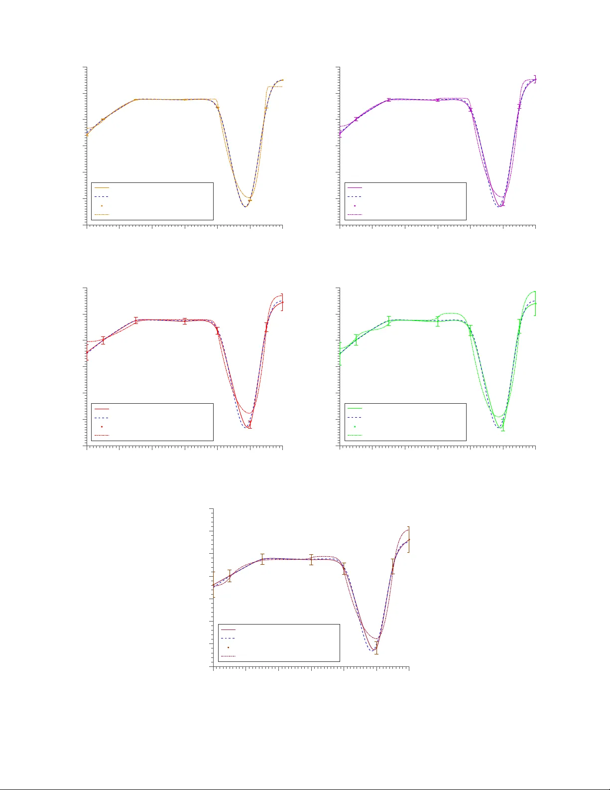
GRADIENT PR OFILE ESTIMA TION USING EXPONENTIAL CUBIC SPLINE SMOOTHING IN A BA YESIAN FRAMEW ORK Kushani De Silv a 1 , Carlo Cafaro 2 , Adom Giffin 3 , 1 Dep artment of Mathematics, Iowa State University, Ames, IA, USA 2 SUNY Polyte chnic Institute, A lb any, NY, USA and 3 CoR.io Inc, Ontario, Ottawa, Canada A ttaining reliable profile gradients is of utmost relev ance for many ph ysical systems. In most situations, the estimation of gradien t can b e inaccurate due to noise. It is common practice to first estimate the underlying system and then compute the profile gradien t by taking the subsequen t analytic deriv ativ e. The underlying system is often estimated by fitting or smo othing the data using other tec hniques. T aking the subsequent analytic deriv ativ e of an estimated function can b e ill-p osed. The ill-p osedness gets worse as the noise in the system increases. As a result, the uncertain ty generated in the gradient estimate increases. In this paper, a theoretical framework for a metho d to estimate the profile gradien t of discrete noisy data is presented. The metho d is dev elop ed within a Ba y esian framew ork. Comprehensiv e numerical exp erimen ts are conducted on synthetic data at different lev els of random noise. The accuracy of the prop osed metho d is quan tified. Our findings suggest that the prop osed gradient profile estimation metho d outperforms the state-of-the-art metho ds. Key words: Computational T ec hniques, Inference Methods, Probability Theory 2 I. INTR ODUCTION Estimating the deriv ative of a system from discrete set of data has a v ast num b er of applications in many fields suc h as biology , engineering, and physics. F or instance, determining the particle velocity from the discrete time-p osition data in particle image velocimetry and particle tracking velocimetry exp eriments [1, 2] are imp ortant tasks in plasma ph ysics [3]. Applications of velocity estimation in motion con trol systems using discrete time data hav e increased with the inv en tion of micropro cessors [4] (and references therein). Moreo ver, with the improv ement of tec hnology , faster equipmen t is now av ailable to measure high-sp eed discrete data [1]. T o estimate the deriv ativ e of a system using discrete data, several approaches ha ve been discussed in the literature. Some of them are finite difference [2] and analytic deriv ativ e of either a traditional data smo othing technique [5 – 12] or Ba yesian data smo othing metho d using spline functions [13–17]. Basically , the latter technique estimates the discrete data using a smo oth function b efore taking the analytic deriv ativ e of the spline function. Most of the time, cubic splines are used as the smo oth function to estimate the discrete data. How ever, as p ointed out in [18, 19], exp onen tial cubic splines are sup erior to cubic splines as they are b etter at capturing in an accurate manner abrupt changes in data. F urthermore, exponential cubic spline is used to directly estimate the unkno wn velocity in [1]. In this case, the spline represent the velocity instead of discrete data as compared to all previous cases. How ever, it is claimed that the noise contaminated in the discrete data can pro duce huge uncertainties in the gradient estimates [4]. These uncertain ties tend to magnify in the gradient estimates when the discrete data are measured in short time interv als, e.g. data captured with high-sp eed cameras [1, 2]. Exp onen tial cubic splines has t wo limiting cases: p olygonal function and cubic spline. These limits are handled b y the smo othing parameter. Therefore, when using exp onen tial cubic spline, sp ecial attention m ust b e paid to the smo othing parameter b ecause extreme v alues of it can sometimes pro duce unrealistic results. The Bay esian approac h emplo yed in the study of [1] used a Jeffrey’s prior on the smo othing parameter simply to scale down the v alue to av oid pro ducing drastic results. Without the optimal smo othness, the spline would not produce optim um gradien t estimates. Moreo ver in that study , the results are stated only for a small level of random noise without a quan titative study of the noise factor. The noise in the data pla ys a ma jor role in this study and a sensitivity analysis of all p ossible noise lev els is imp ortant. F urthermore, the results in p ositions, velocity , and acceleration are not quantitativ ely ev aluated for sup eriority in Ref. [1]. In our study , motiv ated b y the imp ortant w ork presen ted in [1], we present a detailed inv estigation on gradient profile estimation by emplo ying exp onential cubic spline smo othing within a Bay esian setting. The exp onential cubic 3 spline and its prop erties are thoroughly studied and a better choice of prior on the smo othing parameters is in tro duced. Moreo ver, a comprehensive study of sensitivity analysis of noise on the gradient estimates is p erformed. Additionally , the results are ev aluated quantitativ ely for p osition, v elo city , and acceleration estimates. The rest of the pap er is organized as follows. Section I I develops the idea of separating spaces with mathematical bac kground. The Bay esian framework of the algorithm is demonstrated in Section I I I. Afterwards, the computational details are presented in Section IV and Section V. In particular, in these sections, our findings are compared to those obtained by means of more traditional metho ds such as smo othing data with subsequen t analytic deriv ative. Our concluding remarks are given in Section VI. Finally , some tec hnical details app ear in App endix A. I I. SEP ARA TING SP ACES IN BA YESIAN CONTEXT T o ov ercome the dilemma of h uge uncertain ties in the gradient estimates of noisy data, the gradien t is directly appro ximated in the space where the gradient resides using the information a v ailable in the space where data lives. Ba yesian metho ds provide the mec hanism to map the information b et ween the tw o spaces, data and gradient, by in tro ducing a mathematical mo del to relate observ able information (data) with the unknown quantit y (gradient) [20– 26]. According to the problem studied in the paper, the data are the p osition x ( t ) of an ob ject measured at discrete times t while the gradient is the velocity v ( t ) of that ob ject. Hence, the mapping b etw een the tw o spaces is obtained b y the tw o basic relationships b etw een p osition and velocity , x ( t ) def = Z v ( t ) dt , and v ( t ) def = d dt x ( t ). (I I.1) Since the gradien t is directly appro ximated in the v elo city space, the mathematical mo del that claims to represent the velocity of the ob ject is placed in the velocity space. Then mapping the information b etw een the p osition and the v elo city is p erformed by integrating the mathematical mo del using the relation depicted in Eq. (II.1). Throughout the pap er, let the space of the gradient (v-space) b e denoted by V and the space of the data (x-space) b e denoted by U . Let the noisy data b e denoted by { t i , x i } n i =1 ∈ U and the mathematical mo del b y M ∈ V . As highligh ted in the Introduction, the exp onen tial cubic spline is capable of capturing abrupt c hanges and therefore it is a better mo del to represent the velocity of a fast moving ob ject [1, 18, 19]. Let us denote the exp onential cubic spline by S v in which the subscript v sp ecifies that the spline, S is placed in V . As any other spline, the exponential cubic spline is defined in piecewise manner b y its function v alues at a set of knot p ositions. Since, in our problem, the spline represents the gradien t/velocity , the function v alues are the velocity v alues defined at the knot p ositions. 4 Let us denote the velocity v alues at the knot positions ξ v i as f v i for i = 1 , 2 , · · · , E v with ξ v 1 = t 1 and ξ v E v = t n . Therefore, the exponential cubic spline for our v ariables, { ξ v i , f v i } E v i =1 defined in the i th in terv al, can b e written as [19, 27], S v i ( t , f v , λ v , ξ v , E v ) def = f v i (1 − h v ) + f v i +1 h v (I I.2) + M v i λ 2 v i  sinh [ µ v i (1 − h v )] sinh ( µ v i ) − (1 − h v )  + M v i +1 λ 2 v i  sinh ( µ v i h v ) sinh ( µ v i ) − h v  with i = 1,..., E v − 1. The quantities h v , µ v i , and M v i in Eq. (I I.2) are defined as, h v def = t − ξ v i ξ v i +1 − ξ v i , µ v i def = λ v i  ξ v i +1 − ξ v i  , and (I I.3) M v i def =  d 2 dt 2 [ S v i ( t , f v , λ v , ξ v , E v )]  t = ξ v i , resp ectiv ely . F urthermore, ξ v def =  ξ v 1 , · · · , ξ v E v  are the p ositions of the knots, f v def =  f v 1 , · · · , f v E v  are the velocity v alues at knots, λ v def =  λ v 1 , · · · , λ v E v − 1  are the tension v alues b etw een tw o knots, and, finally , E v are the num ber of knots of the spline. Throughout the pap er, the subscript v of the v ariables sp ecifies that they are placed in V . Using the arrow notations for vectorial quantities, the exp onential cubic spline in Eq. (I I.2) can b e also viewed in matrix form as [1], S v  ~ t  = W  ~ t , ~ λ v , ~ ξ v  ~ f v . (I I.4) In Eq. (I I.4), W denotes the design matrix of ~ t -lo cations of the data p oints ~ t , the ~ t -lo cations of the supp ort p oints ~ ξ v , the vector of tension parameters ~ λ v and, finally , the vector of function v alues ~ f v . Moreov er, the quan tity S v is the solution to the v ariational problem [1], Z t n t 1 (  d 2 S v ( t ) dt 2  2 + λ ( t ) 2  dS v ( t ) dt  2 ) dt for ξ i ≤ t ≤ ξ i +1 . (I I.5) The second deriv ativ e of S v , i.e. M v , can b e explicitly found b y solving the tri-diagonal system of equations in Eq. (I I.4). The function v alues ~ f v , the tension v alues ~ λ v , the p ositions of the knots ~ ξ v and the n umber of knots E v are unkno wn. Therefore, a summary of data and parameters of the mo del b eing inv estigated is given in T able I. T ABLE I: The definition of data and parameters of the system data ~ t and ~ x parameters ~ f v , ~ λ v , ~ ξ v and E v ∈ Z + The data resides in U and the parameters of the mo del resides in V is matched using the relation given in Eq. (I I.1) with the purp ose of establishing the connection b et ween the tw o spaces U and V . In fact, it matches data p oints in 5 0 2 4 6 8 10 12 Time (a.u.) -5 0 5 V elo cit y (a.u.) 0 2 4 6 8 10 12 Time (a.u.) 0 10 20 30 P osition (a.u.) FIG. 1: An example of solving a forward problem from a velocity curve (left) to calculate p ositions/distances (right). The v elo city curve is the exp onential cubic spline computed at ~ ξ = [0 , 1 , 3 , 6 , 8 , 10 , 11 , 12]. The p ositions were calculated from the v elo city using the forward problem at n = 13 different time instances. The time axis is given at arbitrary units (a.u.). U with the spline values in V in tegrated ov er time. The relation in Eq. (I I.1) can b e rewritten in terms of our mo del without loss of generality for an arbitrary i th p osition as, x i = Z t i t 1 S v ( t , f v , λ v , ξ v , E v ) dt , (I I.6) with S v ( t , f v , λ v , ξ v , E v ) given in Eq. (I I.2). The quantit y x i in Eq. (I I.6) can b e further reduced to, x i = x i − 1 + Z t i t i − 1 S v i − 1 ( t , f v , λ v , ξ v , E v ) dt , (I I.7) with i = 1, · · · , n . W e p oint out that the exp onential cubic spline is analytically integrable and some technical details are given in App endix A. When a mathematical mo del is used to match the unknown quantit y and the observ able data, the mo del should b e able to generate data as lik ely as p ossible to the observ able information if the desired/unkno wn quan tity is known. This is called the forwar d pr oblem in Bay esian language. Ho w ever, what is required here is to b e able to solve the inverse pr oblem . That is, making inferences ab out the desired/unknown quantit y using the observ ed information and the mo del [28–30]. An example of solving a forw ard problem by computing p ositions when the velocity is known is sho wn in Fig. 1. 6 I I I. THE BA YESIAN RECIPE The inv erse problem for the p osition-velocity scenario introduced in the previous section can b e solved by means of Bay es’ rule, p (v elo city ∈ V | p ositions ∈ U ) = p (v elo city ∈ V ) p (p ositions ∈ U | v elo city ∈ V ) p (p ositions ∈ U ) (I I I.1) The relation depicted in Eq. (I I I.1) shows how the join t p osterior probability distribution can b e built to infer the v elo city when the p ositions are given. Bay es’ rule in Eq. (I I I.1) can b e rewritten using data and parameters given in T able I as follows, p  ~ f v , ~ λ v , ~ ξ v , E v | ~ t , ~ x , I  = p ( ~ f v , ~ λ v , ~ ξ v , E v | I ) p ( ~ x | ~ f v , ~ λ v , ~ ξ v , E v , ~ t , I ) p ( ~ x | I ) , (I II.2) where the quantit y I represents all the relev ant information that concerns the physical scenario under inv estigation together with the a v ailable kno wledge about the experiment b eing p erformed. By assuming the indep endence in spline v ariables, the following relation is satisfied, p ( ~ f v , ~ λ v , ~ ξ v , E v | I ) = p  ~ f v | I  p  ~ λ v | I  p  ~ ξ v | I  p ( E v | I ) . (I I I.3) Substituting Eq. (I I I.3) in to Eq. (I I I.2), we get p  ~ f v , ~ λ v , ~ ξ v , E v | ~ t , ~ x , I  (I I I.4) = p  ~ f v | I  p  ~ λ v | I  p  ~ ξ v | I  p ( E v | I ) p ( ~ x | ~ f v , ~ λ v , ~ ξ v , E v , ~ t , I ) p ( ~ x | I ) . The evidence p ( ~ x | I ) in Eq. (I I I.1) and (I I I.2) is given by , p ( ~ x | I ) def = (I I I.5) Z Z Z Z p  ~ f v | I  p  ~ λ v | I  p  ~ ξ v | I  p ( E v | I ) p ( ~ x | ~ f v , ~ λ v , ~ ξ v , E v , ~ t , I ) d ~ f v d ~ λ v d ~ ξ v dE v , where the likelihoo d distribution is given by p ( ~ x | ~ f v , ~ λ v , ~ ξ v , E v , ~ t , I ). The lik eliho o d distribution affirms the relation b et ween the data and the spline v alues. Since the p osition data x i with i = 1,..., n is contaminated with noise, omitting the arrow notation for v ectorial quantities, Eq. (I I.7) can b e rewritten including the noise term as, x i =                            x 1 + P i − 1 γ =1 R ξ v γ +1 ξ v γ S v γ ( t , f v , λ v , ξ v , E v ) dt + R t i ξ v i S v i ( t , f v , λ v , ξ v , E v ) dt +  i , for ξ v i < t i < ξ v i +1 x 1 + P i − 1 γ =1 R ξ v γ +1 ξ v γ S v γ ( t , f v , λ v , ξ v , E v ) dt +  i , for t i = ξ v i , (I I I.6) 7 where the noise vector ~  def = (  1 ,...,  n ) is assumed to b e linear and, in addition, is assumed to b e Gaussian-distributed with ~  ∼ N ( ~ µ, Σ) . (I I I.7) In Eq. (I I I.7), the quantit y ~ µ is the ( n × 1)-dimensional mean vector while Σ is a ( n × n )-dimensional cov ariance matrix of the noise. F urthermore, the noise is assumed to b e uncorrelated. In other w ords, Σ is a diagonal matrix with diagonal elements giv en by { σ 1 , · · · , σ n } . It is also assumed that ~ µ = ~ 0. F rom Eq. (I I I.6), the following equation can b e written for the i -th noise term,  i = x i − x 1 + i − 1 X γ =1 Z ξ v γ +1 ξ v γ S v γ ( t , f v , λ v , ξ v , E v ) dt + Z t i ξ v i S v i ( t , f v , λ v , ξ v , E v ) dt ! , (I II.8) where i = 1, · · · , n . The symbols S v γ and S v i denote the exp onen tial spline function in Eq. (II.2) in the γ th and the i th sub-in terv als, resp ectively . Assuming that for all i = 1,..., n the data v alues are indep endent and identically distributed, the likelihoo d distribution can b e rewritten as p ( ~ x | ~ f v , ~ λ v , ~ ξ v , E v , ~ t , I ) = n Y i =1 p ( x i | ~ f v , ~ λ v , ~ ξ v , E v , t i , I ). (I I I.9) Com bining Eqs. (I I I.8) and (I I I.9) together with the additional assumption that σ i = σ e =constan t for any 1 ≤ i ≤ n , the likelihoo d distribution b ecomes (case I of Eq. (I I I.6) is assumed here for generality), p ( ~ x | ~ f v , ~ λ v , ~ ξ v , E v , ~ t , I ) = n Y i =1 1 p 2 π σ 2 e exp  − 1 2 σ 2 e (  i ) 2  =  2 π σ 2 e  − n/ 2 exp n X i =1    − 1 2 σ 2 e " x i − x 1 + i − 1 X γ =1 Z ξ v γ +1 ξ v γ S v γ ( · ) dt + Z t i ξ v i S v i ( · ) dt !# 2    =  2 π σ 2 e  − n/ 2 exp n X i =1 G ( x i , ~ f v , ~ λ v , ~ ξ v , E v , ~ t ), (I II.10) with G ( x i , ~ f v , ~ λ v , ~ ξ v , E v , ~ t ) def = − 1 2 σ 2 e " x i − x 1 + i − 1 X γ =1 Z ξ v γ +1 ξ v γ S v γ ( · ) dt + Z t i ξ v i S v i ( · ) dt !# 2 . (I II.11) When the n umber of knots is known ahead of time, the pro duct of prior distributions in Eq. (I I I.3) can b e rewritten as p ( ~ f v , ~ λ v , ~ ξ v , E v | I ) = p  ~ f v | E v , I  p  ~ λ v | E v , I  p  ~ ξ v | E v , I  . (I II.12) 8 A. The c hoice of prior probabilit y distributions The shap e of the curv e pro duced b etw een knots dep ends on the v alues of ~ λ v . One of the concerns with the tension parameter is that it is a scale parameter and it can assume any real n umber. The shap e of the curve b etw een t wo knots can change from cubic function to a p olygonal function when its v alue go es from 0 to ∞ [19, 27]. A polygonal function is not a go o d representation of a moving ob ject due to its lack of smo othness. Th us, the v alue of the tension pla ys a big role in getting the p erfect velocity curve as explained b y the observed data. Therefore, prior distributions on λ v should b e chosen carefully to control its v alue. Previous works in the literature [19, 31] has used Jeffreys’ prior to scale down large v alues pro duced for the tension. In this pap er, w e ha ve employ ed a Gaussian distribution as a prior for the tension. It allows the choice of sensible v alues with a higher probability and non-sensible v alues with a low er probability . A b on us of choosing a Gaussian prior is that it is a conjugate prior of the Gaussian likelihoo d and, as a consequence, makes the resulting p osterior a mem b er of a family of the Gaussian distributions. Assuming iden tical and indep endent tension parameters ~ λ v , the prior distribution p ( ~ λ v | E v , I ) in Eq. (I I I.12) can b e written as p ( ~ λ v | E v , I ) = E v − 1 Y i =1 p ( λ v i | E v , I ) = E v − 1 Y i =1 1 q 2 π σ 2 θ λ i exp " − ( λ v i − µ i ) 2 2 σ 2 θ λ i # =  2 π σ 2 θ λ  − ( E v − 1) / 2 exp " − E v − 1 X i =1 ( λ v i − µ i ) 2 2 σ 2 θ λ # (I I I.13) (b y taking σ θ λ i = σ θ λ ∀ i with 1 ≤ i ≤ E v − 1), with µ i and σ θ λ represen ting the mean and the standard deviation of the parameter λ v i . The prior distributions p  ~ f v | E v , I  and p  ~ ξ v | E v , I  in Eq. (I I I.12) are assumed to b e constant as no prior information on the b ehavior w as iden tified. Finally , using Eqs. (I I I.10) and (I I I.14), the p osterior distribution p  ~ f v , ~ λ v , ~ ξ , E v | ~ t , ~ x , I  in Eq. (I I I.2) can b e viewed as, p  ~ f v , ~ λ v , ~ ξ , E v | ~ t , ~ x , I  ∝ p  ~ λ v | E v , I  p ( ~ x | ~ f v , ~ λ v , ~ ξ , E v , ~ t , I ) ∝  2 π σ 2 θ λ  − ( E v − 1) / 2+( − n/ 2) (I I I.14) exp " − E v − 1 X i =1 ( λ v i − µ i ) 2 2 σ 2 θ λ + n X i =1 G  x i , ~ f v , ~ λ v , ~ ξ , E v , ~ t  # where G ( x i , ~ f v , ~ λ v , ~ ξ v , E v , ~ t ) is given in Eq. (I I I.11). 9 IV. METHODOLOGY Syn thetic data of time-p ositions were generated from the same velocity curve used in the forw ard problem shown in Fig. 1, characterized by a reasonably large sample size with n = 121. Then, the Gaussian noise with µ = 0 and σ w as added to the data, x ( t ) = x true ( t ) + [ µ + z σ ] , (IV.1) with z b eing the standard parameter in tro duced when dealing with normalized Gaussian data sets. F ollo wing from the p osterior distributions defined in Section II I, the n um b er of parameters of the system is determined by E v . F urthermore, when the p ositions and the n umber of knots are provided by the user, the total n umber of parameters of the system will b e 2 E v − 1. F or the syn thetic data, following the w ork in Ref. [27], we select E v = 8 knots at ~ ξ v = [0 , 1 , 3 , 6 , 8 , 10 , 11 , 12] in to inferring the spline. Then, the p osterior distribution with different priors (see Eq. (I II.5)) w ere simulated using a h ybrid MCMC algorithm called DRAM [32]. The simulation b egins with an initial minimization pro cess of the negativ e of the posterior distributions. The initial v alues of the parameters used were, f v initial = 0, and λ v initial = 0 . 001 . (IV.2) W e remark that the posterior distribution is undefined at λ v = 0 and, in addition, the smallest v alue that MA TLAB [33] could handle for λ v w as exp erimentally found to b e equal to 0 . 001. The initial minimization acts as a jump start to the DRAM algorithm. The prop osal distributions of the parameters in DRAM that generate the candidate sample v alues are Gaussian distributions. The user must input v alues for the paramete rs of the prop osal distributions (i.e., mean and v ariance of Gaussian distributions) as given in T able II with LB and U B b eing the low er and upp er b ounds of the parameters, resp ectively . T ABLE II: Initial pr op osal distributions of the system p ar ameters. parameter prop osal distribution prior distribution f v i for i = 1 , · · · , E v Gaussian( µ v i , σ 2 v i ) ∈ ( LB v i , U B v i ) µ θ v i , σ θ v i λ v i for i = 1 , · · · , E v − 1 Gaussian( µ λ i , σ 2 λ i ) ∈ ( LB λ i , U B λ i ) µ θ λ i , σ θ λ i The optimum v alues ~ f v ∗ and ~ λ v ∗ determined by the initial minimization were used as the mean v alues of the 10 prop osal distributions, so that the initial prop osal distributions are centered around ~ f v ∗ and ~ λ v ∗ . The information of prior distributions can b e sp ecified with prior means µ θ v i , µ θ λ i and prior v ariances σ θ v i , σ θ λ i . The DRAM pro cedure tak es the v ariance of the prior as the initial v ariance of the parameters if the co v ariance matrix is not sp ecified by the user. When the prior v ariance is infinit y , the v ariances of the prop osal distributions are calculated as, σ 2 v i = ( µ v i × 0 . 05) 2 , and σ 2 λ i = ( µ λ i × 0 . 05) 2 . (IV.3) In other words, if no prior information is av ailable ab out the parameter, 5% of the mean of the initial distribution is tak en as the initial v ariance. Finally , samples were drawn from these Gaussian prop osals and the marginal densities of the parameters were computed. The MCMC simulations were run until conv ergence was observed. Eac h sampling pro cedure of length MCMCnsim u w as rep eated MCMCN = 100 times. At each of the MCMCN-th rep etitions, the random noise with the same mean and the same standard deviation as reported in Eq. (IV.1) w as added. Hence, a differen t set of data with the same level of noise was used at eac h iteration. At each MCMCN-th rep etition, the initial minimization pro cess was newly ran. All the sample chains were stored and, in addition, the first few samples w ere destroy ed using a MCMCnsimu ∗ p % burn-in p erio d. The quantit y p denotes the burn-in time parameter and, in our case is sp ecified by the in terv al (0 , 100). The av erage marginal densities w ere then computed for each parameter using the remaining samples. In what follows, we assume that nsimu denotes the remaining n umber of samples after burn-in p erio d, that is, nsimu def = (1 − p )% ∗ MCMCnsimu. Then, for any k = 1, · · · , E v , the mean v alues  f ∗ v k  of those mean marginal densities were calculated as, f ∗ v k def = 1 nsim u nsimu X i =1 f v ki , (IV.4) where f v ki denote the av erage sample v alues of f v k after MCMCN num b er of iterations, f v ki def = 1 MCMCN MCMCN X j =1 f v kij . (IV.5) F ollo wing the same line of reasoning presented for Eqs. (IV.4) and (IV.5), we also ha ve λ ∗ v s def = 1 nsim u nsimu X i =1 λ v si = 1 nsim u × MCMCN nsimu X i =1 MCMCN X j =1 λ v sij , (IV.6) for any s = 1, · · · , E v − 1 with λ v si denoting the av erage sample v alues of tension after MCMCN num b er of iterations, λ v si def = 1 MCMCN MCMCN X j =1 λ v sij . (IV.7) Finally , the standard deviations  σ ∗ v k  and  σ ∗ λ s  of the parameters are calculated from the av erage of all chains after 11 MCMCN iterations as, σ ∗ v k def = v u u t 1 nsim u − 1 nsimu X i =1  f v ki − f ∗ v k  2 , (IV.8) for any k = 1, · · · , E v and, σ ∗ λ s def = v u u t 1 nsim u − 1 nsimu X i =1  λ v si − λ ∗ v s  2 , (IV.9) for any s = 1, · · · , E v − 1, resp ectiv ely . V. RESUL TS This section presen ts the results obtained from the metho d explained in the previous sections. The sensitivity of gradien t estimates on the noise levels of the position data are tested. The noise levels on x-space is depicted in Fig. I I with different noise lev els are denoted by σ e . The noise of same level was added randomly at the b eginning of the optimization pro cess with keeping all other v ariables same: The data size n , the num b er of knots of the exp onential cubic spline E v , the p ositions of the knots ~ ξ v , the num b er of MCMC iterations MCMCN, and the true data p ositions. The added noise hav e five different levels of σ e ∈ { 0 . 001, 0 . 3, 0 . 7, 1 . 0, 1 . 3 } from a standard Gaussian distribution. By the definition of the Gaussian distribution, the first four noise levels ha ve a probability of 68 . 2% while the last noise level has a probabilit y of 95%.The noise levels are selected so that that they represent distinct p ossibilities of the Gaussian noise. The sensitivity of noise levels was in vestigated for the p osterior distribution with the Gaussian prior used for the tension parameter. These results of the sensitivity analysis were compared against a common traditional metho d of fitting the same type of exp onential cubic spline in U and the gradien t is obtained b y analytically differentiating the resulting fitted spline function. The notation “ i -fit ( i -space) with i = x, v” denotes the fact that the i -fit was fitted on the i -space where the x-fit is the distance profile while the v-fit is the gradien t profile. A constant force is observed betw een the times 0 − 8( a.u. ) and short impulses are observed b etw een the times 8 − 11( a.u. ). Moreov er, it is observ ed that as the noise level increases, the data around the short impulses tends to get fuzzier so that it is hard to identify the tra jectory . The marginalized p osterior distributions for each parameter is sim ulated using MCMC sampling. When the noise increases, the width of the marginal distributions w ere expanded. This, in turn, resulted in an increased length of the error bars of the parameter estimates. The marginal probability distribution of f v 1 is sho wn in Fig. 3. These uncertainties of the f v i parameters are shown as error bars in Fig. 4 12 -2 0 2 4 6 8 10 12 14 Time (a.u.) -5 0 5 10 15 20 25 30 Distance profile (a.u.) Data ( x ± 0 . 001) Groundtruth pro fi le -2 0 2 4 6 8 10 12 14 Time (a.u.) -5 0 5 10 15 20 25 30 Distance profile (a.u.) Data ( x ± 0 . 3) Groundtruth pro fi le -2 0 2 4 6 8 10 12 14 Time (a.u.) -5 0 5 10 15 20 25 30 Distance profile (a.u.) Data ( x ± 0 . 7) Groundtruth pro fi le -2 0 2 4 6 8 10 12 14 Time (a.u.) -5 0 5 10 15 20 25 30 Distance profile (a.u.) Data ( x ± 1 . 0) Groundtruth pro fi le -2 0 2 4 6 8 10 12 14 Time (a.u.) -5 0 5 10 15 20 25 30 Distance profile (a.u.) Data ( x ± 1 . 3) Groundtruth pro fi le FIG. 2: The panel of time-p osition data with error bars at fiv e differen t noise lev els. Noise levels increase from left to righ t and top to b ottom. The length of error bars is relative to the magnitude of the noise. 13 -4 -3 -2 -1 0 1 2 3 4 5 6 Sample (a.u.) 0 0.02 0.04 0.06 0.08 0.1 0.12 Probability σ e = 1 . 3 σ e = 1 . 0 σ e = 0 . 7 σ e = 0 . 3 σ e = 0 . 001 FIG. 3: The comparison of marginal probability densities of f v 1 parameter at all noise leve ls. 0 2 4 6 8 10 12 Time (a.u.) -6 -4 -2 0 2 4 6 8 Velocity profile (a.u.) v- fi t (v-space) at σ e = 0 . 001 v- fi t (v-space) at σ e = 0 . 3 v- fi t (v-space) at σ e = 1 . 0 v- fi t (v-space) at σ e = 0 . 7 v- fi t (v-space) at σ e = 1 . 3 Ground truth 0 2 4 6 8 10 12 Time (a.u.) -6 -4 -2 0 2 4 6 8 Velocity profile (a.u.) v- fi t (v-space) at σ e = 1 . 3 v- fi t (v-space) at σ e = 1 . 0 v- fi t (v-space) at σ e = 0 . 7 v- fi t (v-space) at σ e = 0 . 3 v- fi t (v-space) at σ e = 0 . 001 Ground truth FIG. 4: The gradient estimates obtained at the five different noise levels. The uncertaint y of the velocity estimates ( ˆ σ v ) are sho wn using error bars (left panel) and credible interv als (right panel). (left panel) and as Bay esian credible interv als in Fig. 4 (right panel). The gradient estimate is obtained at all noise lev els b y placing the mo del in V and is shown in Fig. 4. The estimates almost ov erlap with the ground truth data at all noise lev els, except at the b oundaries and around the time t = 10 a.u. , where the short impulses were presen t in the p osition profile. The uncertainties of b oth v elo city and tension parameters are characterized in Fig. 5. The uncertain ty of the v elo city parameters with the noise lev el exhibits a linear relationship reflecting the linear relationship of velocity parameters in the likelihoo d function. The uncertaint y of the tension parameters do es not show any sp ecific pattern as it has a non linear pattern in the likelihoo d. The gradient estimates are compared with the analytic deriv ativ e of the x-fit obtained in U . The x-fit is obtained by fitting the same exp onen tial cubic spline to the time-p osition data in U . This was p erformed at the same knot p ositions. The gradient profile, the acceleration profile, and p osition profile w ere obtained from the tw o metho ds (via v-fit from V and x-fit from U ) and compared in Fig. 6, Fig. 7 and Fig. 8, resp ectiv ely . The t wo types of estimates of acceleration profile from the v-space and the x-space were obtained b y 14 0 0.2 0.4 0.6 0.8 1 1.2 1.4 Noise level 0 0.2 0.4 0.6 0.8 1 1.2 Uncertainty v 1 v 2 v 3 v 4 v 5 v 6 v 7 v 8 0 0.5 1 1.5 Noise level 0 0.1 0.2 0.3 0.4 0.5 0.6 0.7 Uncertainty λ 1 λ 2 λ 3 λ 4 λ 5 λ 6 λ 7 FIG. 5: The relationship betw een uncertaint y of the estimates and the noise level of the system. The left panel depicts the relationship of velocity parameters whereas the right panel shows the relationship of tension parameters. T ABLE II I: The comparison of accuracy of velocity fit from v space, and x space. || e || 2 noise level v-fit Deriv ative of x-fit 0 . 001 0 . 2077 14 . 4107 0 . 3 1 . 9679 15 . 0792 0 . 7 3 . 1793 20 . 9974 1 3 . 1569 30 . 1122 1 . 3 3 . 8159 31 . 2719 differen tiating the v-fit (v-space) and by finite differencing the v-fit (x-space), resp ectively , from Fig. 6. The gradient estimates that emerge from the tw o spaces (namely , the x-space and v-space) clearly sho w some remark able differences. In particular, the difference in accuracy is shown in T able I I I using the error norm, || e || 2 def = L X i =1  f v estimated i − f v true i  2 , (V.1) where L is the sample size [34]. The acceleration characterizes the acting forces on the ob ject. The acceleration estimate (x-space) could not ac hieve constan t force where it is exp ected. The errors at short impulses around t = 10 a.u. started getting v ery large and this indicates the p ossibility of infinite forces. Moreov er, the acceleration profile from the x-space (red dashed-dot lines) is not realistic with its v ery sharp turns. Therefore, the acceleration estimate from the velocity space is a reliable estimator of acting forces. The goo dness of the fit is tested by studying the error sum of squares (SSE) defined as 15 0 2 4 6 8 10 12 Time (a.u.) -6 -4 -2 0 2 4 6 Velocity profile (a.u.) v- fi t (v-space) at σ e = 0 . 001 Ground truth gradient pro fi le Infered supp ort p oints ( v i ± ˆ σ v i ) Deriv ative pro fi le 0 2 4 6 8 10 12 Time (a.u.) -6 -4 -2 0 2 4 6 Velocity profile (a.u.) v- fi t (v-space) at σ e = 0 . 3 Ground truth gradient pro fi le Infered supp ort p oints ( f i ± ˆ σ v i ) Deriv ative pro fi le 0 2 4 6 8 10 12 Time (a.u.) -6 -4 -2 0 2 4 6 Velocity profile (a.u.) v- fi t (v-space) at σ e = 0 . 7 Ground truth gradient pro fi le Infered supp ort poi nts ( v i ± ˆ σ v i ) Deriv ative pro fi le 0 2 4 6 8 10 12 Time (a.u.) -6 -4 -2 0 2 4 6 Velocity profile (a.u.) v- fi t (v-space) at σ e = 1 . 0 Ground truth gradient pro fi le Infered supp ort p oints ( f i ± ˆ σ v i ) Deriv ative pro fi le 0 2 4 6 8 10 12 Time (a.u.) -6 -4 -2 0 2 4 6 8 Velocity profile (a.u.) v- fi t (v-space) at σ e = 1 . 3 Ground truth gradient pro fi le Infered supp ort p oints ( f i ± ˆ σ v i ) Deriv ative pro fi le FIG. 6: The panel of velocity estimates from the t wo spaces compared at five different noise levels. The noise level increases from left to right and top to b ottom. 16 0 2 4 6 8 10 12 Time (a.u.) -10 -5 0 5 10 15 Acceleration profile (a.u.) Groundtruth acceleration pro fi le Estimated acceleration pro fi le (v-space) at σ e = . 001 Estimated acceleration pro fi le (x-space) at σ e = . 001 0 2 4 6 8 10 12 Time (a.u.) -10 -5 0 5 10 15 Acceleration profile (a.u.) Groundtruth acceleration pro fi le Estimated acceleration pro fi le (v-space) at σ e = 0 . 3 Estimated acceleration pro fi le (x-space) at σ e = 0 . 3 0 2 4 6 8 10 12 Time (a.u.) -10 -5 0 5 10 15 Acceleration profile (a.u.) Groundtruth acceleration pro fi le Estimated acceleration pro fi le (v-space) at σ e = 0 . 7 Estimated acceleration pro fi le (x-space) at σ e = 0 . 7 0 2 4 6 8 10 12 Time (a.u.) -10 -5 0 5 10 15 Acceleration profile (a.u.) Groundtruth acceleration pro fi le Estimated acceleration pro fi le (v-space) at σ e = 1 . 0 Estimated acceleration pro fi le (x-space) at σ e = 1 . 0 0 2 4 6 8 10 12 Time (a.u.) -10 -5 0 5 10 15 Acceleration profile (a.u.) Groundtruth acceleration pro fi le Estimated acceleration pro fi le (v-space) at σ e = 1 . 3 Estimated acceleration pro fi le (x-space) at σ e = 1 . 3 FIG. 7: The panel of acceleration estimates obtained from tw o metho ds are compared at five differen t noise levels. 17 -2 0 2 4 6 8 10 12 14 Time (a.u.) -5 0 5 10 15 20 25 30 Distance profile (a.u.) Data ( x + σ e ) Groundtruth pro fi le x- fi t (v-space) Infered p oints ( f i ± σ i ) x- fi t (x-space) -2 0 2 4 6 8 10 12 14 Time (a.u.) -5 0 5 10 15 20 25 30 Distance profile (a.u.) Data ( x + σ e ) Groundtruth pro fi le x- fi t (v-space) x- fi t (x-space) Infered p oints ( f i ± σ i ) -2 0 2 4 6 8 10 12 14 Time (a.u.) -5 0 5 10 15 20 25 30 Distance profile (a.u.) Data ( x + σ e ) Groundtruth pro fi le x- fi t (v-space) x- fi t (x-space) Infered p oints ( f i ± σ i ) -2 0 2 4 6 8 10 12 14 Time (a.u.) -5 0 5 10 15 20 25 30 Distance profile (a.u.) Data ( x + σ e ) Groundtruth pro fi le x- fi t (v-space) x- fi t (x-space) Infered p oints ( f i ± σ i ) -2 0 2 4 6 8 10 12 14 Time (a.u.) -5 0 5 10 15 20 25 30 Distance profile (a.u.) Data ( x + σ e ) Groundtruth pro fi le x- fi t (v-space) x- fi t (x-space) Infered p oints ( f i ± σ i ) FIG. 8: The panel of x-fit estimates obtained from tw o different spaces compared at five differen t noise levels. 18 T ABLE IV: The comparison of the quality of x-fit from x and v spaces resp ectively using error sum of squares (SSE). SSE with noisy data SSE with true data σ e x-fit ( U ) x-fit ( V ) x-fit ( U ) x-fit ( V ) 0 . 001 1 . 1743 0 . 6082 1 . 1753 0 . 6089 0 . 3 12 . 4677 12 . 6049 2 . 1946 0 . 8541 0 . 7 62 . 4582 63 . 4059 4 . 1855 0 . 8176 1 . 0 121 . 0864 120 . 8161 13 . 3478 1 . 1253 1 . 3 163 . 1339 264 . 3176 18 . 9582 3 . 1651 [35], SSE def = n X i =1  ˆ f i − f i  2 (V.2) where ˆ f i represen t the estimated function v alues. The quantit y f i in Eq. (V.2) is replaced with noisy f i to obtain the second and the third columns in T able IV while f i is replaced with the original f i without noise to calculate the fourth and fifth columns in the same table. The tra jectory estimate is a b onus pro duct from the gradient profile (v-space) and is obtained by integrating the gradient estimate (v-space). The tra jectory estimates (p osition profiles) are compared in Fig. 8. The x-fit (x-space) follows the noisy data closely . This is because when fitting a curve in the same space as data, that curve is trying to minimize the SSE which means it tries to match the data as m uch as p ossible. Therefore, the x-fit from U tries to satisfy the noisy data as muc h as p ossible. How ev er, the x-fit (v-space) follo ws the ground truth data more than it follows the noisy data. When integrating the v-fit (v-space), an additional order of differentiabilit y is added to the tra jectory estimate. Therefore, the x-fit (v-space) has a higher order of differen tiability than that of the x-fit (x-space). This additional order of differentiabilit y ensures the con tinuit y of the velocity and, therefore, it satisfies the constraint of the finite force of the ob ject. The c alculated squared sum of errors (SSE) with true data and noisy data are sho wn in the T able IV. The SSE v alues for noisy data are smaller for the x-fit (x-space). This, in turn, reflects the fact that the x-fit (x-space) follows noisy data b etter. How ever, the SSE v alues for true data are smaller for the x-fit (v-space). This fact, instead, reflects the fact that the x-fit (v-space) follo ws true data better. 19 VI. CONCLUSION In this pap er, we prop osed a metho d to compute the profile gradient of a noisy system using Bay esian inference strategy . The Bay esian inference metho d allow ed the inference of an un-observ able quan tity , the gradient (velocity), b y building a meaningful relationship b et ween the un-observ able gradient profile in one space (that is, the velocity space) and the observ able data profile in another space (that is, the data space - U ). F urthermore, the gradient profile was mo deled by the exp onential cubic spline. The results of this new metho d are compared against a common metho d of fitting an exp onential cubic spline in data space ( U ) and taking the subsequent analytic deriv ative. The fitting in U was also p erformed in a Bay esian framework and the same DRAM sampler was used to sim ulate the p osterior distributions. The results show that the gradient estimates obtained by mo deling in v-space pro duce more accurate estimates than the results of the traditional metho d (see T able I I I). Moreov er, it was able to pro duce b etter acceleration estimates with reliable and accurate v alues where a constan t force is exp ected (see FIG. 7). The third t yp e of estimate, the tra jectory profile w as also compared. W e conclude that the x-fit estimates follow noisy data when solved by placing the mo del in the x-space while the x-fit estimates follo ws the ground truth data when solved placing the mo del in the velocity space (see FIG. 8 and T able IV). It is argued that b y integrating the mo del in v elo city space, an extra order of differentiabilit y is added to x-fit ensuring the finite force constraint of a moving ob ject. In conclusion, the metho d demonstrated in this paper is a sup erior metho d to estimate the velocity of a mo ving ob ject under finite force as compared to others in literature (for instance, see [1] and references therein). It ensured b etter estimates in all three cases: tra jectory , v elo city , and the acceleration. W e p oint out that although our main focus in this pap er is on the proposal of a nov el theoretical method to estimate a profile gradient from discrete noisy data, a num b er of improv emen ts can b e sought in its practical implementation. F or instance, the use of an MCMC algorithm gains precision at the expense of speed. A faster algorithm (such as the Exp ectation Maximization algorithm [36]) may b e needed for real time estimation. F urthermore, the amount and placemen t of the knots lacks a systematic guiding principle. In the future we plan to use Bay esian mo del selection for determining the amoun t. F or the placemen t issue, w e can adopt a hierarchical approach b y including spline knot location algorithms [37] in conjunction with our main algorithm. This would provide estimates for the v alues asso ciated with the knots and where they should b e lo cated as w ell. Finally , w e hop e to apply our Bay esian estimation tec hnique to more realistic problems where acceleration, velocity , and tra jectory estimations are needed. The authors w ould like to thank the meaningful and helpful discussions had with Udo V on T oussain t at the Max- 20 Planc k Institute in Garc hing, Germany . [1] U. von T oussain t and S. Gori, Digital p article image velo cimetry using splines in tension , AIP Conf. Proc. 1305, 337 (2011). [2] Y. F eng, J. Goree, and B. Liu, Err ors in p article tr acking velo cimetry with high-sp e e d camer as , Review of Scien tific Instru- men ts 82, 053707 (2011). [3] M. A. Chilenski, M. Greenw ald, Y. Marzouk, N. T. How ard, A. E. White, J. E. Rice, and J. R. W alk, Improve d pr ofile fitting and quantific ation of uncertainty in exp erimental me asur ements of impurity tr ansp ort c o efficients using Gaussian pr o c ess r e gr ession , Nuclear F usion 55, 023012 (2015). [4] R. H. Brown, S. C. Schneider, and M. G. Mulligan, Analysis of algorithms for velo city estimation fr om discr ete p osition versus time data , IEEE T ransactions on Industrial Electronics 39, 11 (1992). [5] C. H. Reinsch, Smo othing by spline functions , Numerische Mathematik 10, 177 (1967). [6] C. H. Reinsch, Smo othing by spline functions. II , Numerische Mathematik 16, 451 (1971). [7] T. J. Hastie and R. J. Tibshirani, Gener alize d additive mo dels , Monographs on Statistics and Applied Probability , v ol. 43 (1990). [8] G. W ahba, Spline mo dels for observational data , SIAM, vol. 59 (1990). [9] M. P W and and M. C. Jones, Kernel Smo othing , CRC Press (1994). [10] P . J. Green and B. W. Silv erman, Nonp ar ametric R egr ession and Gener alize d Line ar Mo dels: A R oughness Penalty Ap- pr o ach , CRC Press (1993). [11] S. W old, Spline functions in data analysis , T ec hnometrics 16, 1 (1974). [12] B. W. Silv erman, Some asp e cts of the spline smo othing appr o ach to non-p ar ametric r e gr ession curve fitting , Journal of the Ro yal Statistical Society B47, 1 (1985). [13] G. W ah ba, Improp er priors, spline smo othing and the pr oblem of guar ding against mo del errors in r e gression , Journal of the Roy al Statistical So ciety B40, 364 (1978). [14] G. S. Kimeldorf and G. W ahba, A c orr esp ondenc e b etwe en Bayesian estimation on sto chastic pr o c esses and smo othing by splines , The Annals of Mathematical Statistics 41, 495 (1970). [15] C. F. Ansley and R. Kohn, Estimation, filtering, and smoothing in state sp ac e mo dels with inc ompletely sp e cifie d initial c onditions , The Annals of Statistics 13, 1286 (1985). [16] S. M. Berry , R. J. Carroll, and D. Ruppert, Bayesian smo othing and re gr ession splines for me asur ement err or pr oblems , Journal of the American Statistical Asso ciation 97, 160 (2002). [17] R. Fischer, K. M. Hanson, V. Dose, and W. von Der Linden, Backgr ound estimation in exp erimental sp e ctr a , Phys. Rev. E61, 1152 (2000). 21 [18] V. Dose and R. Fischer, F unction estimation employing exponential splines , AIP Conf. Pro c. 803, 67 (2005). [19] R. Fisc her and V. Dose, Flexible and r eliable pr ofile estimation using exp onential splines , AIP Conf. Proc. 872, 296 (2006). [20] T. Bay es, An Essay towar ds Solving a Pr oblem in the Do ctrine of Chanc es. By the L ate R ev. Mr. Bayes, F. R. S. Com- munic ate d by Mr. Pric e, in a L etter to John Canton, A. M. F. R. S , Philosophical T ransactions of the Roy al So ciety of London 53, 370 (1763). [21] G. E. P . Bo x and G. C. Tiao, Bayesian Infer enc e in Statistic al Analysis , vol. 40, John Wiley & Sons (2011). [22] J. Gewek e, Bayesian infer enc e in e c onometric mo dels using Monte Carlo inte gr ation , Econometrica 57, 1317 (1989). [23] A. P . Dempster, A generalization of Bayesian infer enc e , Journal of the Roy al Statistical So ciety B30, 205 (1968). [24] D. Gamerman and H. F. Lop es, Markov Chain Monte Carlo: Stochastic Simulation for Bayesian Infer enc e , CRC Press, 2006. [25] D. C. Knill and W. Richards, Per c eption as Bayesian Infer enc e , Cambridge Univ ersit y Press (1996). [26] M. A. Newton and A. E. Raftery , Appr oximate Bayesian infer enc e with the weighte d likeliho o d b o otstr ap , Journal of the Ro yal Statistical Society B56, 3 (1994). [27] P Rentrop, An algorithm for the c omputation of the exp onential spline , Numerische Mathematik 35, 81 (1980). [28] A. Mohammad-Djafari, Bayesian infer enc e for inverse pr oblems , AIP Conf. Pro c. 617, 477 (2002). [29] D. Sivia and J. Skilling, Data Analysis: A Bayesian T utorial , Oxford Universit y Press (2006). [30] A. Gelman, J. B. Carlin, H. S. Stern, and D. B. Rubin, Bayesian Data Analysis , vol. 2, T a ylor & F rancis (2014). [31] R. Fischer, A. Dinklage, and Y. T urkin, Non-p ar ametric profile gr adient estimation , in the 33rd EPS Conference on Plasma Ph ys. Rome, 19 - 23 June 2006 ECA V ol. 30I, P-2.127 (2006). [32] H. Haario, M. Laine, A. Mira, and E. Saksman, DRAM: Efficient adaptive MCMC , Statistics and Computing 16, 339 (2006). [33] MA TLAB, version R2015b, The MathW orks Inc. (2015). [34] P . C. Hansen, Analysis of discr ete il l-p ose d pr oblems by me ans of the L-curve , SIAM Review 34, 561 (1992). [35] M. Merriman, A text b ook on the Metho d of L east Squar es , John Wiley & Sons (1909). [36] A. P . Dempster, N. M. Laird, and D. B. Rubin, Maximum likeliho o d from inc omplete data via the EM algorithm , Journal of the Roy al Statistical So ciety , Series B39 (Metho dological), 1-38 (1977). [37] E. L. Monto ya, N. Ulloa, and V. Miller, A simulation study c omp aring knot sele ction metho ds with e qual ly sp ac e d knots in a p enalize d r e gr ession spline , Int. J. Statistics and Probability 3, 96 (2014). 22 App endix A In this App endix, we present some details on the integration of the exp onential cubic spline. The in tegration is done in tw o cases. In one case, one in tegrates the spline function b etw een tw o knots and it is referred to as I full . In the other case, one integrates the spline function from a knot to a random p oint b efore the next knot and it is referred to as I partial . The t wo types of integrals yield, I full = Z ξ v k +1 ξ v k S v ( t , f v , λ v , ξ v , E v ) dt , (A.1) with k = 1, · · · , E v − 1, and I partial = Z t i ξ v k S v ( t , f v , λ v , ξ v , E v ) dt (A.2) with k = 1, · · · , E v − 1, i = 1, · · · , n , and ξ v k ≤ t i < ξ v k +1 , resp ectiv ely . The solutions to these tw o cases presented in Eq. (A.1) and Eq. (A.2) can b e found analytically and result in the following expressions, I partial = f v i +1 2 h v i ( t i − ξ v i ) 2 + f v i ( t i − ξ v i ) 2 h v i (2 ξ v i +1 − t i − ξ v i ) (A.3) − M v i ( t i − ξ v i ) 2 λ 2 v i h v i (2 ξ v i +1 − t i − ξ v i ) + M v i λ 3 v i sinh( λ v i h v i )  cosh( λ v i h v i ) − cosh  λ v i ( t i − ξ v i +1 )  + M v i +1 λ 3 v i sinh( λ v i h v i ) { cosh [ λ v i ( t i − ξ v i )] − 1 } − M v i +1 2 λ 2 v i h v i ( t i − ξ v i ) 2 , (A.4) and, I full = f v i h v i 2 + f v i +1 h v i 2 − M v i h v i 2 λ 2 v i − M v i +1 h v i 2 λ 2 v i + ( M v i +1 + M v i ) λ 3 v i tanh  λ v i h v i 2  . (A.5) App endix B In this App endix, b eing in the framework of Mark ov c hain Monte Carlo (MCMC) methods, we presen t some details on the Delay ed Rejection Adaptive Metropolis (DRAM) algorithm used to compute p osterior distributions in our w ork. DRAM is a hybrid algorithm where the concepts of Delay ed Rejection (DR) and Adaptive Metropolis (AM) are combined for enhancing the pe rformance of the Metrop olis-Hastings (MH) type MCMC algorithms [32]. In the basic MH algorithm, up on the rejection of the new candidate at a (j + 1)th state, the sample remains at the current p oin t (j). How ever, when the Dela yed Rejection is introduced, upon rejection, another new candidate z is drawn. Then, one finds out whether it can b e accepted. The AM feature, instead, is a global adaptive strategy which is combined 23 with the partial lo cal adaptation caused b y the DR strategy . The idea of AM is to tune the prop osal distribution at eac h time step dep ending on the past. In other words, the cov ariance matrix of the prop osal distribution dep ends on the history of the sample chain (sequence of samples). Usually the adaptation starts after an initial p erio d of time (0, t). Algorithm 1 DRAM 1: for j = 1 : N do 2: Generate y from q  Θ ( j ) , .  and u from U (0 , 1) 3: if y is outside ( L, U ) then 4: Reject y (level 1) 5: else 6: Calculate α 1 (Θ ( j ) , y ) 7: if u ≤ α 1 (Θ ( j ) , y ) then 8: Θ ( j +1) = y 9: else 10: Reject y (level 2) { starts dela yed rejection } 11: Generate new candidate z from q ( y , . ) 12: if z is outside ( L, U ) then 13: Reject z (level 3) 14: else 15: Calculate α 2 (Θ ( j ) , y , z ) and u from U (0 , 1) 16: if u ≤ α 2 (Θ ( j ) , y , z ) then 17: Θ ( j +1) = z 18: else 19: Reject z (level 4) 20: Θ ( j +1) = Θ ( j ) 21: end if 22: end if 23: end if 24: end if 25: end for 26: Return the v alues { Θ (0) , Θ (1) , Θ (2) , · · · , Θ ( N ) } . 24 The basic steps of the DRAM algorithm is giv en in Algorithm 1 with an arbitrary initial p oint Θ (0) . The acceptance probabilities at steps 6 and 15 are shown in Eqs. (B.1a) and (B.1b) resp ectively . α 1 ( x, y ) =          min h π ( y ) q ( y ,x ) π ( x ) q ( x,y ) , 1 i if π ( x ) q ( x, y ) > 0 , 1 otherwise . (B.1a) α 2 ( x, y , z ) =                  min h π ( z ) π ( x ) q ( z ,y ) q ( x,y ) q ( z,y ,x ) q ( x,y,z ) [1 − α 1 ( z ,y )] [1 − α 1 ( x,y )] , 1 i if π ( x ) q ( x, y ) q ( x, y , z ) [1 − α 1 ( x, y )] > 0 , 1 otherwise . (B.1b) q ( θ ) represents the prop osal distribution and Θ ( j ) represen ts the set of parameters of the prop osal distribution at j-th iteration.