A Probabilistic Calculus of Cyber-Physical Systems

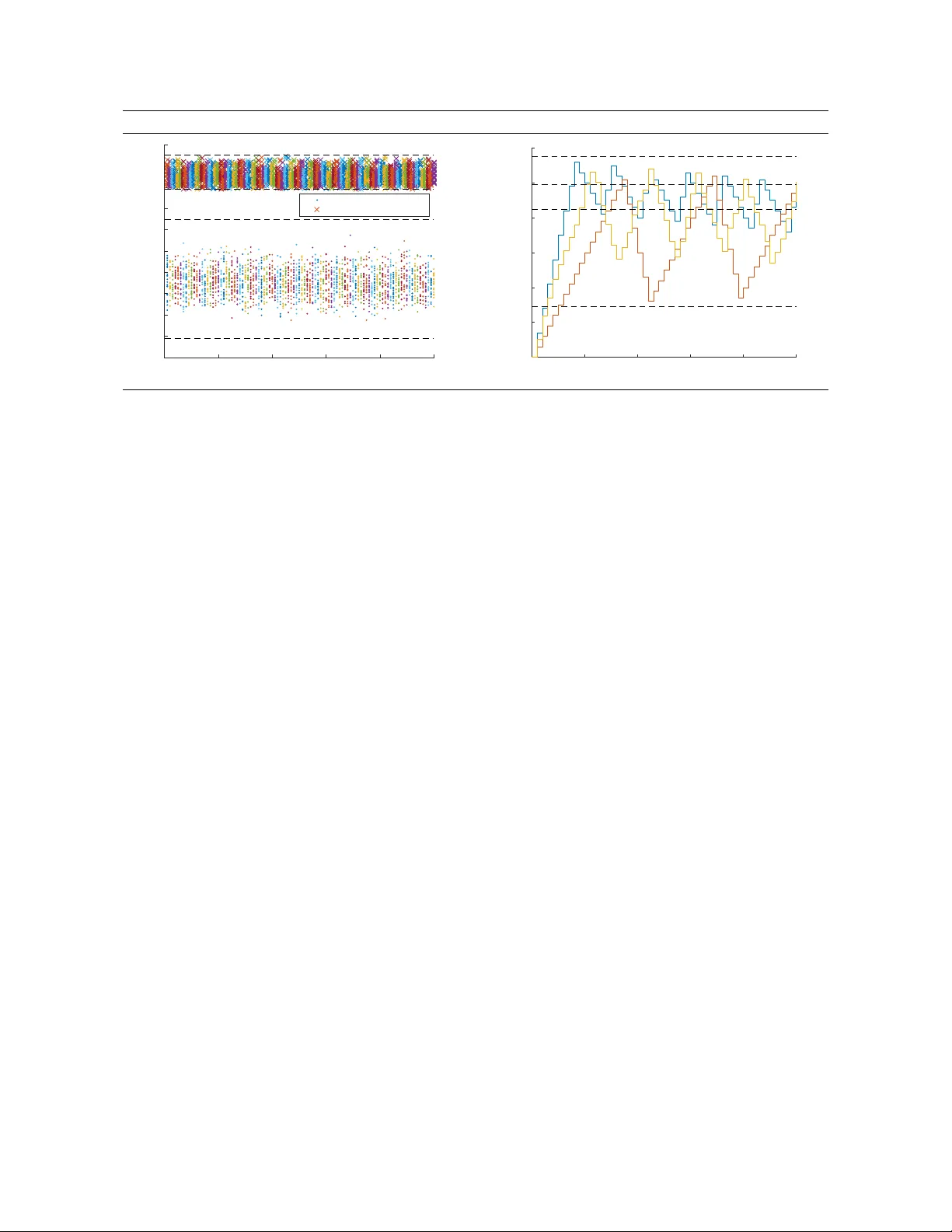
Submitted to: Information and Computation c  R. Lanotte, M. Merro, S. T ini This work is licensed under the Creativ e Commons Attribution License. A Pr obabilistic Calculus of Cyber -Ph ysical Systems ∗ Ruggero Lanotte Dipartimento di Scienza e Alta T ecnologia Univ ersit ` a degli Studi dell’Insubria, Como, Italy Massimo Merro Dipartimento di Informatica Univ ersit ` a degli Studi di V erona, Italy Simone T ini Dipartimento di Scienza e Alta T ecnologia Univ ersit ` a degli Studi dell’Insubria, Como, Italy Cyber-Physical Systems (CPSs) are integrations of networking and distributed computing systems with physical processes, where feedback loops allo w physical processes to af fect computations and vice versa. Although CPSs can be found in sev eral real-world domains (automoti ve, a vionics, energy supply , etc), their veriﬁcation often relies on simulation test systems rather then formal methodologies . This is because there is still a lack of research on the modelling and the deﬁnition of formal semantics to compare non-trivial CPSs in terms of their runtime beha viours up to an acceptable tolerance . W e propose a hybrid pr obabilistic pr ocess calculus for modelling and reasoning on cyber -physical systems (CPSs). The dynamics of the calculus is expressed in terms of a pr obabilistic labelled tran- sition system in the SOS style of Plotkin. This is used to deﬁne a bisimulation-based probabilistic behavioural semantics which supports compositional reasonings. For a more careful comparison between CPSs, we provide two compositional pr obabilistic metrics to formalise the notion of be- havioural distance between systems, also in the case of bounded computations. Finally , we provide a non-trivial case study , taken from an engineering application, and use it to illustrate our deﬁnitions and our compositional behavioural theory for CPSs. 1 Intr oduction Cyber-Physical Systems (CPSs) are integrations of networking and distrib uted computing systems with physical processes, where feedback loops allow ph ysical processes to affect computations and vice v ersa. CPSs can be considered as an ev olution of embedded systems , where components are immersed in and interact with the physical w orld, via physical de vices (such as sensors and actuators ). They can also be seen as an ev olution of networked contr ol systems , where physical processes and controllers interact via a communication system. The physical plant of a CPS is often represented by means of a discr ete-time state-space model 1 consisting of two equations of the form x k + 1 = Ax k + Bu k + w k y k = Cx k + e k where x k ∈ R n is the current (physical) state , u k ∈ R m is the input (i.e., the control actions implemented through actuators) and y k ∈ R p is the output (i.e., the measurements obtained from the sensors). The uncertainty w k ∈ R n and the measur ement err or e k ∈ R p represent perturbation and sensor noise, respec- ti vely . The parameters A , B , and C are matrices modelling the dynamics of the physical system. The ne xt state x k + 1 depends on the current state x k and the corresponding control actions u k , at the sampling instant k ∈ N . Note that, the state x k cannot be directly observed: only its measurement y k can be observed. ∗ A preliminary version appeared in the proceedings of LA T A 2017, LNCS 10168, pp. 115-127, Springer [44]. 1 W e refer to [64] for a taxonomy of time-scale models used to represent CPSs. 2 A Probabilistic Calculus of Cyber-Ph ysical Systems Figure 1 Structure of a CPS Actuators Plant ? w k Sensors ? e k Controller - - x k y k  u k - The physical plant is supported by a communication network through which the sensor measurements and actuator data are exchanged with the contr oller(s) , i.e., the cyber component, also called logics, of a CPS (see Figure 1). In general terms, CPSs can be considered as both nondeterministic and pr obabilistic systems. Nonde- terminism arises as they consist of distributed networks in which the activities of speciﬁc components occur nondeterministically , whereas the probabilistic beha viour is due to the presence of the uncertainty in the model and the measurement error , which are usually represented as pr obability distributions . The range of CPSs applications is rapidly increasing and already cov ers se veral domains [ 41 ]: adv anced automotiv e systems, energy conserv ation, en vironmental monitoring, avionics, critical infras- tructure control (for instance, electric po wer , water resources, and communications systems), etc. Ho wev er, there is still a lack of research on the modelling and v alidation of CPSs through formal methodologies that allo w us to model the interactions among the system components, and to verify the correctness of a CPS, as a whole, before its practical implementation. A straightforward utilisation of these techniques is for model-chec king [ 17 ], or e ven better , for pr obabilistic model-checking [ 42 ], to statically assess whether the current system deployment can guarantee the expected beha viour . Ho we ver , they can also be an important aid for system planning, for instance to decide whether different deplo yments for a gi ven application are beha viourally equi v alent. Process calculi hav e been successfully used to model and analyse concurrent, distributed and mobile systems (see, e.g., the π -calculus [ 50 ], Ambients [ 14 ] and the Distributed π -calculus [ 38 ]). Howe ver , to better describe systems based on a particular paradigm, dedicated calculi are needed. Hybrid process algebr as [ 18 , 7 , 57 , 54 , 30 ] ha ve been proposed for reasoning about physical systems and provide techniques for analysing and v erifying protocols for hybrid automata. In order to enrich h ybrid models with probabilistic or stochastic beha viour, a number of different approaches have been proposed in the last years [ 56 , 39 , 12 , 2 , 29 , 36 , 62 ]. Ho wev er, to our knowledge, none of these formalisms provide bisimulation metrics semantics to estimate the deviation in terms of behaviour of dif ferent CPSs in a process-algebra setting. The deﬁnition of these instruments represents the main goal of the current paper . Contribution. In this paper , we propose a hybrid pr obabilistic pr ocess calculus , called pCCPS ( Pr oba- bilistic Calculus of Cyber -Physical Systems ), with a clearly-deﬁned pr obabilistic behavioural semantics for specifying and reasoning on CPSs. In pCCPS , cyber-physical systems are represented by making a neat distinction between the physical component describing the physical process (consisting in state v ariables, sensors, actuators, evolution law , measurement law , etc.) and the cyber component , i.e., the logics (i.e., controllers, IDS, supervisors, etc.) that gov erns sensor reading and actuator writing, as well as channel-based communication with other cyber components. Thus, channels are used for logical interactions between cyber components, whereas sensors and actuators make possible the interaction between cyber and physical components. Despite this conceptual similarity , messages transmitted via R. Lanotte, M. Merro, S. Tini 3 channels are “consumed” upon reception, whereas actuators’ states (think of a valve) remains unchanged until its controller modiﬁes it. pCCPS adopts a discr ete notion of time [ 37 ] and it is equipped with a pr obabilistic labelled transition semantics (pL TS) in the style of [ 55 ]. W e prove that our probabilistic labelled transition semantics satisﬁes some standard time properties such as: time determinism , patience , maximal pr ogr ess , and well-timedness . Based on our pL TS, we deﬁne a natural notion of weak pr obabilistic bisimilarity , written ≈ . As a main result, we prov e that bisimilarity in pCCPS is preserved by appropriate system contexts and it is hence suitable for compositional r easoning . Then, we provide a non-tri vial case study , tak en from an engineering application, and use it to illustrate our deﬁnitions and our compositional behavioural theory for CPSs. W e also use our case study to sho w that the probabilistic bisimilarity is only partially satisfactory to reason on CPSs as it can only establish whether two CPSs behave exactly in the same way or not. An y tiny v ariation of the probabilistic beha viour of one of the two systems under consideration will break the equality without any further information on the “distance” of their behaviours. T o this end, bisimulation metric semantics ha ve been successfully employed to formalise the behaviour al distance between two systems [ 27 , 26 , 59 , 21 ]. W e generalise our probabilistic bisimilarity by providing a notion of weak bisimulation metric for pCCPS along the lines of [ 27 ]. W e will write M ≈ p N , if the weak bisimilarity between CPSs M and N holds with a distance p , with probability p ∈ [ 0 , 1 ] . Intuitively , ≈ 0 will coincide with the weak probabilistic bisimilarity ≈ , whereas S p ∈ [ 0 , 1 ] ≈ p will correspond to the cartesian product pCCPS × pCCPS . W e also provide a notion of n -bisimilarity metric which takes into account bounded computations of systems [ 26 ]. This kind of metric, denoted with ≈ n p , for n ∈ N + , says that the distance p of the systems under considerations is ensured only for the ﬁrst n computation steps. Said in other words, if M ≈ n p N then for the ﬁrst n computation steps the runtime behaviour of systems M and N may dif fer with pr obability at most p . Both metrics ≈ p and ≈ n p are prov ed to be preserved by the same contexts considered for ≈ , and hence the y re veal to be suitable for compositional reasonings. In particular , they satisfy a well-kno wn compositional property called non-expansiveness [ 26 , 31 , 33 ], the analogue of the congruence property of weak bisimulation. Finally , with the help of our case study , we will show ho w n -bisimilarity metric can be v ery helpful in situations where it is not necessary to observe a system “ad inﬁnitum” as it makes much more sense to observ e its behaviour for bounded computations. Outline. In Section 2, we give syntax and operational semantics of pCCPS . In Section 3, we provide a bisimulation-based probabilistic behavioural semantics for pCCPS and prove its compositionality . In Section 4, we model our case study in pCCPS , and prov e for it run-time properties as well as system equalities. In Section 5, we deﬁne bisimulation metrics for pCCPS . In Section 6, we revise our case study by providing a more accurate analysis based on the proposed bisimulation metrics. In Section 7, we draw conclusions and discuss related and future work. 2 The calculus In this section, we introduce our Pr obabilistic Calculus of Cyber-Physical Systems , pCCPS . Let us start with some preliminary notations. W e use x , x k ∈ X for state variables (associated to physical states of systems), c , d ∈ C for communication channels , a , a k ∈ A for actuator devices , s , s k ∈ S for sensors devices . Actuator names are metav ariables for actuator devices like valve , light , etc. Similarly , sensor names are metav ariables for sensor de vices, e.g., a sensor thermometer that measures a state v ariable called temperatur e , with a giv en precision. V alues , ranged ov er by v , v 0 ∈ V , are built from basic v alues, such as Booleans, integers and real numbers; they also include names. Giv en a generic set of 4 A Probabilistic Calculus of Cyber-Ph ysical Systems names N , we write R N to denote the set of functions assigning a real v alue to each name in N . For ξ ∈ R N , n ∈ N and v ∈ R , we write ξ [ n 7→ v ] to denote the function ψ ∈ R N such that ψ ( m ) = ξ ( m ) , for any m 6 = n , and ψ ( n ) = v . Given ξ 1 ∈ R N 1 and ξ 2 ∈ R N 2 such that N 1 ∩ N 2 = / 0 , we denote with ξ 1 ] ξ 2 the function in R N 1 ∪ N 2 such that ( ξ 1 ] ξ 2 )( n ) = ξ 1 ( n ) , if n ∈ N 1 , and ( ξ 1 ] ξ 2 )( n ) = ξ 2 ( n ) , if n ∈ N 2 . As pCCPS is a probabilistic calculus, we report the necessary mathematical machinery for its formal deﬁnition. Deﬁnition 1 (Probability distribution) . A (discrete) probability sub-distribution over a set of generic objects O is a function δ : O → [ 0 , 1 ] with ∑ o ∈ O δ ( o ) ∈ ( 0 , 1 ] . W e write | δ | as an abbr eviation for ∑ o ∈ O δ ( o ) . The support of a pr obability sub-distribution δ is given by supp ( δ ) = { o ∈ O : δ ( o ) > 0 } . W e write D sub ( O ) , rang ed over γ , δ and ε , for the set of all ﬁnite-support pr obability sub-distributions over the set O . A pr obability sub-distribution δ ∈ D sub ( O ) is said to be a probability distribution if ∑ o ∈ O δ ( o ) = 1 . W ith D ( O ) we denote the set of all ﬁnite-support pr obability distributions o ver O . F or any o ∈ O , the point (Dirac) distribution at o , denoted o , assigns pr obability 1 to o and 0 to all others elements of O , so that supp ( o ) = { o } . Let I be a ﬁnite indexing set such that (i) δ i is a sub-distribution in D sub ( O ) for each i ∈ I , and (ii) p i ≥ 0 are probabilities such that ∑ i ∈ I p i ∈ ( 0 , 1 ] . The probability sub-distrib ution (or con ve x combination) ∑ i ∈ I p i · δ i is the sub-distribution deﬁned by ( ∑ i ∈ I p i · δ i )( o ) = ∑ i ∈ I p i δ i ( o ) for all o ∈ O . W e write a sub-distribution as p 1 · δ 1 + . . . + p k · δ k when the indexing set I is { 1 , . . . , k } . In pCCPS , a cyber -physical system consists of: • a physical component (deﬁning physical variables, ph ysical de vices, physical e volution, etc.) and • a cyber (or logical) component that interacts with the physical devices (sensors and actuators) and communicates via channels with other cyber components. Physical components in pCCPS are giv en by two sub-components: (i) the physical state , which is supposed to change at runtime, and (ii) the physical en vir onment , which contains static information. 2 Deﬁnition 2 (Physical state) . Let X be a set of state variables, S be a set of sensors, and A be a set of actuators. A physical state S is a triple h ξ x , ξ s , ξ a i , wher e: • ξ x ∈ R X is the state function , • ξ s ∈ R S is the sensor function , • ξ a ∈ R A is the actuator function . All functions deﬁning a physical state ar e total . The state function ξ x returns the current v alue associated to each v ariable in X . The sensor function ξ s returns the current v alue associated to each sensor in S ; similarly , the actuator function ξ a returns the current v alue associated to each actuator in A . Deﬁnition 3 (Physical en vironment) . Let X be a set of state variables, S be a set of sensors, and A be a set of actuators. A physical en vironment E is a triple h e vol , meas , in v i , where: • e vol : R X × R A → D ( R X ) is the ev olution map , • meas : R X → D ( R S ) is the measurement map , • in v ∈ 2 R X is the in variant set . All the functions deﬁning a physical en vir onment ar e total functions . 2 Actually , this information is periodically updated (say , every six months) to tak e into account possible drifts of the system. R. Lanotte, M. Merro, S. Tini 5 Gi ven a state function and an actuator function, the evolution map evol returns a pr obability distribution over state functions . This function models the evolution law of the physical system, where changes made on actuators may reﬂect on state variables. Since we assume the presence of a known (maximal) uncertainty for our models, the e v olution map does not return a speciﬁc state function b ut a probability distribution ov er state functions. Gi ven a state function, the measurement map meas returns a pr obability distribution over sensor functions . Also in this case, since we assume the presence of a known (maximal) measurement error for each sensor , the measurement map returns a probability distribution o ver sensor functions, rather than a speciﬁc sensor function. The in variant set in v returns the set of state functions that satisfy the in variant of the system. A CPS that gets into a physical state with a state function that does not satisfy the in variant is in deadloc k . Let us no w formalise the cyber components of CPSs in our calculus pCCPS . Our (logical) processes build on Hennessy and Re gan’ s T imed Pr ocess Language TPL [ 37 ] (basically CCS enriched with a discrete notion of time). W e extend TPL with three constructs: one to read values detected at sensors, one to write v alues on actuators, and one to e xpress (guarded) probabilistic choice. The remaining processes of the calculus are the same as those of TPL. Deﬁnition 4 (Processes) . Processes ar e deﬁned by the grammar: P , Q :: = nil   tick . C   P k Q   b chn . C c D   phy . C   [ b ] { P } , { Q }   P \ c   X   rec X . P C , D :: = L i ∈ I p i : P i chn :: = snd c h v i   rcv c ( x ) phy :: = read s ( x )   write a h v i . W e write nil for the terminated pr ocess . The process tick . C models sleeping for one time unit. W e write P k Q to denote the parallel composition of concurrent processes P and Q . The process b chn . C c D , with chn ∈ { snd c h v i , rcv c ( x ) } , denotes channel transmission with timeout . Thus, b snd c h v i . C c D sends the value v on channel c and, after that, it continues as C ; otherwise, if no communication partner is av ailable within one time unit, it ev olves into D . The process b rcv c ( x ) . C c D is the obvious counterpart for channel reception. Processes of the form phy . C denote activities on physical devices (sensors or actuators). Thus, the construct read s ( x ) . C reads the v alue v detected by the sensor s and, after that, it continues as C , where x is replaced by v . The process write a h v i . C writes the value v on the actuator a and then it continues as C . The process P \ c is the channel restriction operator of CCS. It is quantiﬁed over the set of communica- tion channels, although we often use the shorthand P \{ c 1 , · · · , c n } to mean P \ c 1 \ c 2 · · · \ c n . The process [ b ] { P } , { Q } is the standard conditional, where b is a decidable guard. For simplicity , as in CCS, we identify process [ b ] { P } , { Q } with P , if b e valuates to true, and [ b ] { P } , { Q } with Q , if b e valuates to f alse. In processes of the form tick . D and b chn . C c D , the occurrence of D is said to be time-guar ded . The process rec X . P denotes time-guar ded recur sion as all occurrences of the process v ariable X may only occur time-guarded in P . The construct L i ∈ I p i : P i denotes pr obabilistic choice , where I is a ﬁnite , non-empty set of index es, and p i ∈ ( 0 , 1 ] , for i ∈ I , denotes the probability to execute the process P i , with ∑ i ∈ I p i = 1 . As in [ 24 ], in order to simplify the operational semantics, pr obabilistic choices occur always underneath pr eﬁxing . In the two constructs b rcv c ( x ) . C c D and read s ( x ) . C , the variable x is said to be bound . Similarly , the process variable X is bound in rec X . P . This giv es rise to the standard notions of free/bound (pr ocess) variables and α -con version . W e identify processes up to α -con version (similarly , we identify CPSs up to 6 A Probabilistic Calculus of Cyber-Ph ysical Systems renaming of state variables, sensor names, and actuator names). A term is closed if it does not contain free (process) variables, and we assume to always work with closed processes: the absence of free variables is preserved at run-time. As further notation, we write T { v / x } for the substitution of the variable x with the v alue v in any e xpression T of our language. Similarly , T { P / X } is the substitution of the process variable X with the process P in T . Everything is in place to pro vide the deﬁnition of cyber -physical systems expressed in pCCPS . Deﬁnition 5 (Cyber-ph ysical system) . F ixed a set of state variables X , a set of sensors S , and a set of actuators A , a c yber-physical system in pCCPS is given by two components: • a physical component consisting of – a physical en vironment E deﬁned on X , S , and A , and – a physical state S r ecording the curr ent values associated to the state variables in X , the sensors in S , and the actuators in A ; • a c yber component P that inter acts with the sensors in S and the actuators A , and can communicate , via channels, with other cyber components of the same or of other CPSs. W e write E ; S o n P to denote the r esulting CPS, and use M and N to rang e over CPSs. Sometimes, when the physical en vir onment E is clearly identiﬁed, we write S o n P instead of E ; S o n P . CPSs of the form S o n P ar e called envir onment-fr ee CPSs. The reader should notice that the syntax of our CPSs is slightly too permissive as a process might use sensors and/or actuators which are not deﬁned in the physical state. Deﬁnition 6 (W ell-formedness) . Let S = h ξ x , ξ s , ξ a i be a physical state, E = h evol , meas , in v i a physical en vir onment, and P a pr ocess. The CPS E ; S o n P is said to be well-formed if: (i) any sensor mentioned in P is in the domain of the function ξ s ; (ii) any actuator mentioned in P is in the domain of the function ξ a . A sub-distribution γ ∈ D sub ( pCCPS ) is said to be well-formed if its support contains only well-formed CPSs. Hereafter , we will always work with well-formed CPSs. As usual in process calculi, we use the symbol ≡ to denote standard structural congruence for timed processes [ 50 , 49 ]; its generalisation to CPSs is immediate: E ; S o n P ≡ E ; S o n Q if P ≡ Q . Also the generalisation to sub-distrib utions in D sub ( pCCPS ) is straightforward: giv en two sub-distrib utions γ and γ 0 ov er CPSs, we write γ ≡ γ 0 if γ ([ M ] ≡ ) = γ 0 ([ M ] ≡ ) for all equiv alence classes [ M ] ≡ ⊆ pCCPS . Finally , we assume a number of notational con ventions . W e write Dead to denote a deadlocked CPS which cannot perform any action. This ﬁctitious CPS will be useful when deﬁning behavioural distances between CPSs (see Deﬁnition 14). W e write chn . P instead of rec X . b chn . P c X , when X does not occur in P . W e write snd c (resp. rcv c ) when channel c is used for pure synchronisation. For k ≥ 0, we write tick k . P as a shorthand for tick . tick . . . . tick . P , where the preﬁx tick appears k consecuti ve times. Giv en a CPS M = E ; S o n P , a process Q and a channel c , we write M k Q for E ; S o n ( P k Q ) , and M \ c for E ; S o n ( P \ c ) . In the rest of the paper, symbol σ ranges ov er distributions ov er physical states, π ranges ov er distributions o ver processes, and γ ranges over distrib utions ov er CPSs. 2.1 Probabilistic labelled transition semantics In this section, we pro vide the dynamics of pCCPS in terms of a pr obabilistic labelled transition system (pL TS) [ 55 ]. First, we giv e a pretty standard probabilistic L TS for processes, then we lift transition rules from processes to CPSs to deal with the probability distributions occurring in ph ysical en vironments. In T able 1, we provide transition rules for processes. Here, the meta-variable λ ranges over labels in the set { tick , τ , cv , cv , a ! v , s ? ( x ) } . These labels denote the passage of time, internal activities, channel R. Lanotte, M. Merro, S. Tini 7 T able 1 Probabilistic L TS for processes (Outp) − b snd c h v i . C c D cv − − → J C K (Inpp) − b rcv c ( x ) . C c D cv − − → J C { v / x } K (Write) − write a h v i . C a ! v − − − → J C K (Read) − read s ( x ) . C s ? ( x ) − − − − → J C K (Com) P 1 cv − − → π 1 P 2 cv − − → π 2 P 1 k P 2 τ − − → π 1 k π 2 (Par) P λ − − → π λ 6 = tick P k Q λ − − → π k Q (ChnRes) P λ − − → π λ 6∈ { cv , cv } P \ c λ − − → π \ c (Rec) P { rec X . P / X } λ − − → π rec X . P λ − − → π (T imeNil) − nil tick − − − → nil (Delay) − tick . C tick − − − → J C K (T imeout) − b chn . C c D tick − − − → J D K (T imePar) P 1 tick − − − → π 1 P 2 tick − − − → π 2 P 1 k P 2 τ − − → 6 P 1 k P 2 tick − − − → π 1 k π 2 transmission, channel reception, actuator writing, and sensor reading, respecti vely . As in [ 24 ], the deﬁnition of the labelled transition relation for processes relies on a semantic interpretation of probabilistic processes in terms of (discrete) probability distributions o ver processes. Deﬁnition 7. F or any pr obabilistic choice L i ∈ I p i : P i over a ﬁnite index set I , we write J L i ∈ I p i : P i K to denote the pr obability distribution ∑ i ∈ I p i · P i . The transition rules in T able 1 use some ob vious notation for distrib uting both parallel composition and channel restriction over a sub-distribution. Gi ven two sub-distributions π 1 and π 2 we deﬁne the sub-distribution π 1 k π 2 as follows: ( π 1 k π 2 )( P ) = π 1 ( P 1 ) · π 2 ( P 2 ) , if P = P 1 k P 2 ; ( π 1 k π 2 )( P ) = 0 , otherwise. Gi ven an arbitrary distribution over processes π = ∑ i ∈ I p i · P i , an arbitrary channel c , and a v alue v , we deﬁne π \ c as the distribution ∑ i ∈ I p i · P i \ c , and π { v / x } as the distribution ∑ i ∈ I p i · P i { v / x } . Let us comment on the transition rules of T able 1. Rules (Outp) , (Inpp) and (Com) serve to model channel communication, on some channel c . Rule (Write) denotes the writing of some data v on an actuator a . Rule (Read) denotes the reading of some value detected at sensor s . Rule (Par) propagates untimed actions ov er parallel components. Rules (ChnRes) and (Rec) are the standard rules for channel restriction and recursion, respectiv ely . The following four rules are standard, and model the passage of one time unit. The symmetric counterparts of rules (Com) and (Par) are obvious and thus omitted from the table. In T able 2, we lift the transition rules from processes to systems, actually to probability distri- butions o vers systems. W e adopt the following notation for probability distributions: gi ven a distri- bution σ ov er physical states and a distribution π ov er processes, we write σ o n π to denote the dis- tribution ov er (en vironment-free) CPSs deﬁned as ( σ o n π )( S o n P ) = σ ( S ) · π ( P ) . Moreov er , gi ven a physical en vironment E , we write E ; σ o n π to extend the distribution σ o n π to full CPSs as follows: ( E ; σ o n π )( E ; S o n P ) = σ ( S ) · π ( P ) . Actions, ranged over by α , are in the set Act = { τ , cv , cv , tick } . These actions denote: non-observable acti vities ( τ ); channel transmission ( cv ); channel reception ( cv ); the passage of time ( tick ). 8 A Probabilistic Calculus of Cyber-Ph ysical Systems T able 2 Probabilistic L TS for a CPS S o n P parametric on an en vironment E = h evol , meas , in v i (Out) P cv − − → π S ∈ in v S o n P cv − − → S o n π (Inp) P cv − − → π S ∈ in v S o n P cv − − → S o n π (T au) P τ − − → π S ∈ in v S o n P τ − − → S o n π (SensRead) P s ? ( z ) − − − − → π ξ s ( s ) = ∑ i ∈ I p i · v i ξ x ∈ in v h ξ x , ξ s , ξ a i o n P τ − − → h ξ x , ξ s , ξ a i o n ∑ i ∈ I p i · π { v i / z } (ActWrite) P a ! v − − − → π ξ x ∈ in v h ξ x , ξ s , ξ a i o n P τ − − → h ξ x , ξ s , ξ a [ a 7→ v ] i o n π (T ime) P tick − − − → π S o n P τ − − → 6 S ∈ in v S o n P tick − − − → next E ( S ) o n π (Deadlock) S 6∈ in v S o n P τ − − → Dead As physical en vironments contain static information, for simplicity the resulting transition rules are parameterised on a physical en vironment of the form E = h evol , meas , inv i . Thus, instead of providing the transitions rules for a CPS of the form E ; S o n P we giv e the L TS semantics parametric on E for the en vironment-free CPS S o n P . All rules, except (Deadlock) , ha ve a common premise requiring that the current state function of the system must satisfy the in variant. W ith an ab use of notation, we sometimes write S ∈ in v instead of ξ x ∈ in v when S = h ξ x , ξ s , ξ a i . Rules (Out) and (Inp) model transmission and reception, with an e xternal system, on a channel c . Rule (T au) lifts non-observ able actions from processes to systems. Rule (SensRead) models the reading of the current data detected at sensor s . Rule (ActWrite) models the writing of a v alue v on an actuator a . A similar lifting occurs in rule (T ime) for timed actions, where next E ( S ) returns a probability distribution ov er possible physical states for the next time slot, according to the current physical state S and physical en vironment E . Formally , for S = h ξ x , ξ s , ξ a i and E = h evol , meas , in v i , we deﬁne: next E ( S ) = ∑ ξ 0 x ∈ supp ( evol ( ξ x , ξ a )) ξ 0 s ∈ supp ( meas ( ξ x 0 ))  evol ( ξ x , ξ a )( ξ 0 x ) · meas ( ξ x 0 )( ξ 0 s )  · h ξ 0 x , ξ 0 s , ξ a i . Intuiti vely , the operator next E serves to compute the possible state functions and sensor functions of the next time slot (actuator changes are go verned by the c yber-component). More precisely , the (probability distribution over the) ne xt state function is determined by applying evol to the current state function ξ x and the current actuator function ξ a . The probability weight of any possible state function ξ 0 x is gi ven by evol ( ξ x , ξ a )( ξ 0 x ) . Then, for a state function ξ 0 x , the (probability distribution o ver the) ne xt sensor function is gi ven by applying meas to ξ 0 x . Finally , the probability weight of any possible sensor function ξ 0 s is gi ven by meas ( ξ 0 x )( ξ 0 s ) . Recapitulating, by an application of rule (T ime) a CPS mov es to the next physical state, in the next time slot. Rule (Deadlock) is straightforward: if the in variant is not satisﬁed then the CPS deadlocks. Finally , notice that in our L TS we deﬁned transitions rules of the form S o n P α − − → σ o n π , parametric on some physical en vironment E . As physical en vironments do not change at runtime, S o n P α − − → σ o n π entails E ; S o n P α − − → E ; σ o n π , thus providing the probabilistic L TS for (full) CPSs. Remark 1. Note that the rules in T able 2 deﬁne an image ﬁnite pLTS. This means that for any CPS M and R. Lanotte, M. Merro, S. Tini 9 label α ther e ar e ﬁnitely many distributions r eachable fr om M in one α -labelled tr ansition step. Moreo ver , all transitions M α − → γ ar e such that γ has a ﬁnite support. No w , ha ving deﬁned the labelled transitions that can be performed by a CPS of the form E ; S o n P , we can easily concatenate these transitions to deﬁne the possible computation traces of a system. A computation trace [ 8 ] for a CPS E ; S 1 o n P 1 is a sequence of steps of the form E ; S 1 o n P 1 α 1 − → . . . α n − 1 − − − → E ; S n o n P n where for any i , with 1 ≤ i ≤ n − 1 , we hav e E ; S i o n P i α i − → E ; σ i + 1 o n π i + 1 for distributions σ i + 1 and π i + 1 such that S i + 1 ∈ supp ( σ i + 1 ) and P i + 1 ∈ supp ( π i + 1 ) . Belo w , we report a few desirable time properties [ 37 ] which hold in our calculus: (a) time determinism , (b) maximal pr ogr ess , (c) patience , and (d) well-timedness . In its standard formulation, time determinism says that a system reaches at most one new state by executing a timed action tick ; howe ver , in our setting, this holds only for the logical components (up to structural congruence) whereas the ev olution of the physical component is intrinsically probabilistic, due to the presence of uncertainty and measurement errors. The maximal pr ogr ess property usually says that processes communicate as soon as a possibility of communication arises. In our calculus, we generalise this property saying that instantaneous (silent) actions cannot be delayed. On the other hand, patience says that if no instantaneous actions are possible then time is free to pass. Finally , well-timedness [ 49 , 15 ] ensures the absence of inﬁnite instantaneous traces which would pre vent the passage of time, and hence the ph ysical ev olution of a CPS. Theorem 1 (T ime properties) . Let M = E ; S o n P. (a) If M tick − − − → γ and M tick − − − → γ 0 then γ ≡ γ 0 . (b) If M τ − − → γ then ther e is no γ 0 such that M tick − − − → γ 0 . (c) If M tick − − − → γ for no γ then either S does not satisfy the in variant of E or ther e is γ 0 such that M τ − − → γ 0 . (d) Ther e is a k ∈ N such that if M α 1 − → . . . α n − → N , with α i 6 = tick , then n ≤ k. The proof of Theorem 1 can be found in the Appendix, in Section A.1. 3 Pr obabilistic bisimulation In this section, we are ready to deﬁne a bisimulation-based behavioural equality for CPSs, relying on our labelled transition semantics. W e recall that the only observable activities in pCCPS are: the passage of time and channel communication. As a consequence, the capability to observe physical e vents (dif ferent from deadlocks) depends on the capability of the cyber components to recognise those events by acting on sensors and actuators, and then signalling them using (unrestricted) channels. In a probabilistic setting, the deﬁnition of weak transition ˆ α = ⇒ , which abstract a way non-observ able actions, is complicated by the fact that (strong) transitions take CPSs to distributions ov er CPSs. Follo wing [24, 47], we need to generalise transitions, so that they tak e sub-distributions to sub-distrib utions. W ith an abuse of notation, we use γ and γ 0 to range over sub-distributions ov er CPSs, under the assumption that ∑ M ∈ pCCPS γ ( M ) ≤ 1. Let us start with deﬁning the weak transition M ˆ α − → γ for any CPS M and distribution γ . If α = τ then we write M ˆ α − → γ whene ver either M α − → γ or γ = M . Otherwise, if α 6 = τ then we write M ˆ α − → γ whene ver M α − → γ . The relation ˆ α − → is extended to model transitions from sub-distributions to sub-distrib utions. For a sub-distrib ution γ = ∑ i ∈ I p i · M i , we write γ ˆ α − → γ 0 if there is a non-empty set J ⊆ I such that M j ˆ α − → γ j for all j ∈ J , M i ˆ α − → 6 , for all i ∈ I \ J , and γ 0 = ∑ j ∈ J p j · γ j . Note that if α 6 = τ then this deﬁnition entails that 10 A Probabilistic Calculus of Cyber-Ph ysical Systems only some CPSs in the support of γ hav e an ˆ α − → transition. Then, we deﬁne the weak transition relation ˆ τ = ⇒ as the transiti ve and reﬂe xiv e closure of ˆ τ − → , i.e. ˆ τ = ⇒ = ( ˆ τ − → ) ∗ , while for α 6 = τ we let ˆ α = ⇒ denote ˆ τ = ⇒ ˆ α − → ˆ τ = ⇒ . In order to deﬁne a probabilistic bisimulation, follo wing [ 23 ] we rely on the notion of matching [ 61 ] (also known as coupling ) for a pair of distributions. Intuitiv ely , the matching for a pair ( γ , γ 0 ) may be understood as a transportation schedule for the shipment of probability mass from γ to γ 0 . Deﬁnition 8 (Matching) . A matching for a pair of distrib utions ( γ , γ 0 ) , with γ , γ 0 ∈ D ( pCCPS ) , is a distribution ω in the pr oduct space D ( pCCPS × pCCPS ) such that: • ∑ M 0 ∈ pCCPS ω ( M , M 0 ) = γ ( M ) , for all M ∈ pCCPS , and • ∑ M ∈ pCCPS ω ( M , M 0 ) = γ 0 ( M 0 ) , for all M 0 ∈ pCCPS . W e write Ω ( γ , γ 0 ) to denote the set of all matchings for ( γ , γ 0 ) . Everything is in place to deﬁne weak probabilistic bisimulation for pCCPS , along the lines of [53]. Deﬁnition 9 (W eak probabilistic bisimulation) . A binary symmetric r elation R over CPSs is a weak probabilistic bisimulation if M R N and M α − − → γ implies that ther e exist a distribution γ 0 and a matching ω ∈ Ω ( γ , γ 0 ) such that N ˆ α = = ⇒ γ 0 , and M 0 R N 0 whenever ω ( M 0 , N 0 ) > 0 . W e say that M and N ar e bisimilar , written M ≈ N , if M R N for some weak pr obabilistic bisimulation R . A main result of the paper is that bisimilarity can be used to reason on CPSs in a compositional manner . In particular , bisimilarity is preserved by parallel composition of physically-disjoint CPSs, by parallel composition of pur e-logical processes, and by channel restriction; basically , all those conte xts that cannot interfere on physical devices (sensors and actuators), whereas interferences on logical components (via channel communication) is allo wed. Intuiti vely , tw o CPSs are physically-disjoint if the y have dif ferent plants but the y may share logical channels for communication purposes. More precisely , physically-disjoint CPSs have disjoint state v ariables and disjoint physical de vices (sensors and actuators). As we consider only well-formed CPSs (Deﬁnition 6), this ensures us that a CPS cannot physically interfere with a parallel CPS by acting on its physical de vices. Although, logical interferences on communication channels are allowed. Formally , let S i = h ξ i x , ξ i s , ξ i a i and E i = h evol i , meas i , in v i i be physical states and physical en vironments, respecti vely , associated to state v ariables in the set X i , sensors in the set S i , and actuators in the set A i , for i ∈ { 1 , 2 } . F or X 1 ∩ X 2 = / 0, S 1 ∩ S 2 = / 0 and A 1 ∩ A 2 = / 0, we deﬁne: • the disjoint union of the physical states S 1 and S 2 , written S 1 ] S 2 , to be the physical state h ξ x , ξ s , ξ a i such that: ξ x = ξ 1 x ] ξ 2 x , ξ s = ξ 1 s ] ξ 2 s , and ξ a = ξ 1 a ] ξ 2 a ; • the disjoint union of the physical en vironments E 1 and E 2 , written E 1 ] E 2 , to be the physical en vironment h evol , meas , in v i such that: ( evol ( ξ 1 x ] ξ 2 x , ξ 1 a ] ξ 2 a ))( ξ 1 x 0 ] ξ 2 x 0 ) = evol 1 ( ξ 1 x , ξ 1 a )( ξ 1 x 0 ) · evol 2 ( ξ 2 x , ξ 2 a )( ξ 2 x 0 ) ( meas ( ξ 1 x ] ξ 2 x ))( ξ 1 s 0 ] ξ 2 s 0 ) = meas 1 ( ξ 1 x )( ξ 1 s 0 ) · meas 2 ( ξ 2 x )( ξ 2 s 0 ) ξ 1 x ] ξ 2 x ∈ in v iff ξ 1 x ∈ in v 1 and ξ 2 x ∈ in v 2 . Deﬁnition 10 (Physically-disjoint CPSs) . Let M i = E i ; S i o n P i , for i ∈ { 1 , 2 } . W e say that M 1 and M 2 ar e physically-disjoint if S 1 and S 2 have disjoint sets of state variables, sensors and actuators. In this case, we write M 1 ] M 2 to denote the CPS deﬁned as ( E 1 ] E 2 ) ; ( S 1 ] S 2 ) o n ( P 1 k P 2 ) . F or any M ∈ pCCPS , the special system Dead is physically-disjoint with M , and M ] Dead = Dead ] M = Dead . R. Lanotte, M. Merro, S. Tini 11 A pure-lo gical pr ocess is a process which may interfere on communication channels b ut it ne ver interferes on physical devices as it ne ver accesses sensors and/or actuators. Basically , a pure-logical process is a (possibly probabilistic) TPL process [ 37 ]. Thus, in a system M k Q , where M is an arbitrary CPS, a pure-logical process Q cannot interfere with the physical ev olution of M . Although, process Q can deﬁnitely interact with M via communication channels, and hence af fect its observable beha viour . Deﬁnition 11 (Pure-logical processes) . A pr ocess P is called pure-logical if it never acts on sensors and/or actuators. No w , we can ﬁnally prov e the compositionality of probabilistic bisimilarity ≈ . Theorem 2 (Congruence results) . Let M and N be two arbitrary CPSs in pCCPS . 1. M ≈ N implies M ] O ≈ N ] O, for any physically-disjoint CPS O; 2. M ≈ N implies M k P ≈ N k P, for any pur e-logical pr ocess P; 3. M ≈ N implies M \ c ≈ N \ c, for any c hannel c. The proof can be found in the Appendix, at the end of Section A.3. The reader may wonder whether the bisimilarity ≈ is preserved by more permissiv e contexts. The answer is no. Suppose to allow in the second item of Theorem 2 a process P that can also read on sensors. In this case, e ven if M and N are bisimilar , the parallel process P might read a dif ferent v alue in the two systems at the v ery same sensor s (due to the sensor error) and transmit these different v alues on a free channel, breaking the congruence. Activities on actuators may also lead to different behaviours of the compound systems: bisimilar CPSs may have physical components that are not exactly aligned. A similar reasoning applies when composing CPSs with non physically-disjoint ones: interference on physical de vices may break the congruence. Ho wev er, in the ne xt section we will see that the congruence results of Theorem 2 will be very useful when reasoning on complex systems. 4 Case study In this section, we provide a case study to illustrate ho w pCCPS can be used to specify and reason on CPSs in a compositional manner . In particular , we model an engine whose temperature is maintained within a speciﬁc range by means of a cooling system. As regards the physical en vir onment we adopt discrete uniform distributions ov er suitable intervals to model both the ev olution map and the measurement map. 3 In our model, we assume a granularity g ∈ N + representing the precision 10 − g of the model in estimating physical values. Thus, for an arbitrary real interv al [ v , w ] we write [ v , w ] g to denote the ﬁnite set of reals { k ∈ [ v , w ] : k = v + h · 10 − g , with h ∈ N } . Gi ven a granularity g ∈ N + , the physical state S g of the engine is characterised by: (i) a state variable temp containing the current temperature of the engine; (ii) a sensor s t (such as a thermometer or a thermocouple) measuring the temperature of the engine, (iii) an actuator cool to turn on/of f the cooling system. The physical en vironment of the engine, En v g , is constituted by: (i) a simple ev olution law evol that increases (resp. decreases) the value of temp , when the cooling system is inactiv e (resp. acti ve), by a v alue determined according to a discrete distribution of probability , taking into account an uncertainty in the model that may reach the threshold δ = 0 . 4 , and granularity g ov er reals; (ii) a measurement map meas returning the value detected by the sensor s t determined by a discrete probability distribution based 3 Other forms of ﬁnite-support discrete probability distributions could be treated as well. 12 A Probabilistic Calculus of Cyber-Ph ysical Systems on a measurement error that may reach the threshold err = 0 . 1 , and granularity g ; (ii) an in v ariant set saying that the system gets faulty when the temperature of the engine gets out of the range [ 0 , 30 ] . Formally , S g = h ξ x , ξ s , ξ a i and Env g = h evol , meas , in v i with: (i) ξ x ∈ R { temp } and ξ x ( temp ) = 0; (ii) ξ s ∈ R { s t } and ξ s ( temp ) = 0; (iii) ξ a ∈ R { cool } and ξ a ( cool ) = oﬀ ; for the sake of simplicity , we can assume ξ a to be a mapping { cool } → { on , oﬀ } such that ξ a ( cool ) = oﬀ if ξ a ( cool ) ≥ 0, and ξ a ( cool ) = on if ξ a ( cool ) < 0. Furthermore, (i) e vol ( ξ 0 x , ξ 0 a ) = ∑ v ∈ [ v 1 , v 2 ] g 1 | [ v 1 , v 2 ] g | · [ temp 7→ ξ 0 x ( t em p ) + v ] , for an y ξ 0 x ∈ R { t em p } and ξ 0 a ∈ R { cool } , where [ v 1 , v 2 ] = [ 1 − δ , 1 + δ ] , if ξ 0 a ( cool ) = oﬀ (inacti ve cooling), and [ v 1 , v 2 ] = [ − 1 − δ , − 1 + δ ] , if ξ 0 a ( cool ) = on (active cooling); (ii) meas ( ξ 0 x ) = ∑ v ∈ [ − err , + err ] g 1 | [ − err , + err ] g | · [ s t 7→ ξ 0 x ( t em p ) + v ] , for any ξ 0 x ∈ R { t em p } ; (iii) in v = { [ temp 7→ x ] : x ∈ R and 0 ≤ x ≤ 30 } . The cyber component of the engine consists of a process Ctrl which models the controller activity . Intuiti vely , process Ctrl senses the temperature of the engine at each time interv al. When the sensed temperature is abov e 10 , the controller activ ates the coolant. The cooling activity is maintained for 5 consecuti ve time units. After that time, if the temperature does not drop below 10 then the controller transmits its ID on a speciﬁc channel for signalling a warning , it keeps cooling for another 5 time units, and then checks again the sensed temperature; otherwise, if the sensed temperature is not abov e the threshold 10, the controller turns of f the cooling and mov es to the next time interv al. Formally , Ctrl = rec X . read s t ( x ) . [ x > 10 ] { Cooling } , { tick . X } Cooling = write cool h on i . rec Y . tick 5 . read s t ( x ) . [ x > 10 ] { snd warning h ID i . Y } , { write cool h oﬀ i . tick . X } . The whole engine is deﬁned as: Eng g = En v g ; S g o n Ctrl , where En v g and S g are the physical en viron- ment and the physical state deﬁned before. Our operational semantics allows us to formally pro ve a number of run-time pr operties of our engine. For instance, the follo wing proposition says that our engine nev er reaches a warning state and ne ver deadlocks. Proposition 1. Let Eng g be the CPS deﬁned befor e. Given any computation Eng g α 1 − → . . . α n − → M , then α i ∈ { τ , tick } , for 1 ≤ i ≤ n, and ther e is a distribution γ suc h that M α − − → γ , for some α ∈ { τ , tick } . Actually , knowing that in each of the 5 time slots of cooling, the temperature will drop of a value laying in the interv al [ 1 − δ , 1 + δ ] g , we can be quite precise on the temperature reached by the engine before and after the cooling acti vity . Formally: Proposition 2. Let Eng g α 1 − − → . . . α n − − → M be an arbitrary computation of the engine, for some CPS M : • if M turns the cooling on then the value of the state variable temp in M r anges over ( 9 . 9 , 11 . 5 ] ; • if M turns the cooling of f then the value of the variable temp in M ranges o ver ( 2 . 9 , 8 . 5 ] . The proofs of both propositions can be found in the Appendix, in Section A.2. The result formally prov ed in Proposition 2 ﬁnds a correspondence in the left graphic of Figure 2. In that graphic, we collect a campaign of 100 simulations of our engine in MA TLAB 4 , lasting 250 time units 4 MA TLAB chooses a v alue in a real interval by means of a discrete uniform distribution depending on the granularity imposed by the ﬁnite number of bits used for the representation of ﬂoats. R. Lanotte, M. Merro, S. Tini 13 Figure 2 Simulations in MA TLAB of the engine Eng experiments 0 20 40 60 80 100 actual temperature (deg) 2 3 4 5 6 7 8 9 10 11 12 switch off cooling system switch on cooling system time 0 10 20 30 40 50 actual temperature (deg) 0 2 4 6 8 10 12 each, sho wing that the v alue of the state variable temp when the cooling system is turned on (resp., off) lays in the interval ( 9 . 9 , 11 . 5 ] (resp., ( 2 . 9 , 8 . 5 ] ); these bounds are represented by the dashed horizontal lines. Ob viously , when dealing with complex systems e ven sev eral thousands of simulations do not ensure the absence of incorrect states, as formally prov ed in Proposition 1 and Proposition 2. The right graphic of the same ﬁgure shows three possible ev olutions in time of the state variable temp : (i) the ﬁrst one (in red), in which the temperature of the engine al ways gro ws of 1 − δ = 0 . 6 degrees per time step, when the cooling is off, and always decrease of 1 + δ = 1 . 4 degrees per time unit, when the cooling is on; (ii) the second one (in blue), in which the temperature always gro ws of 1 + δ = 1 . 4 degrees per time unit, when the cooling is off, and always decrease of 1 − δ = 0 . 6 degrees per time unit, when the cooling is on; (iii) and a third one (in yello w), in which, depending whether the cooling is of f or on, at each time step the temperature gro ws or decreases of an arbitrary offset laying in the interv al [ 1 − δ , 1 + δ ] . No w , the reader may wonder whether it is possible to design a v ariant of our engine which meets the same speciﬁcation with better performances. For instance, an engine consuming less coolant. Let us consider a v ariant of the engine described before: ] Eng g = g En v g ; S g o n Ctrl . Here, g En v g is the same as En v g except for the ev olution map, as we set [ v 1 , v 2 ] = [ − 0 . 8 − δ , − 0 . 8 + δ ] if ξ 0 a ( cool ) = on (acti ve cooling). This means that in ] Eng g we reduce the po wer of the cooling system by 20% . In Figure 3, we report the results of our simulations in MA TLAB o ver 10000 runs lasting 10000 time units each. From this graph, ] Eng g sav es in a verage more than 10% of coolant with respect to Eng g . So, the ne w question is: are these two engines beha vioural equi v alent? Do they meet the same speciﬁcation? Our bisimilarity provides us with a precise answer to these questions: the two v ariants of the engine are bisimilar . Proposition 3. Eng g ≈ ] Eng g , for any g ∈ N + . The proof can be found in the Appendix, in Section A.4. At this point, one may wonder whether it is possible to improve the performances of our engine e ven more. F or instance, by reducing the po wer of the cooling system by a further 10% , by setting [ v 1 , v 2 ] = [ − 0 . 7 − δ , − 0 . 7 + δ ] if ξ 0 a ( cool ) = on (acti ve cooling). W e can formally prov e that this is not possible. Proposition 4. Let [ Eng g be the same as Eng g , except for the evolution map, in which the r eal interval [ v 1 , v 2 ] is given by [ − 0 . 7 − δ , − 0 . 7 + δ ] if ξ 0 a ( cool ) = on . Then, Eng g 6≈ [ Eng g , for any g ∈ N + . 14 A Probabilistic Calculus of Cyber-Ph ysical Systems Figure 3 Simulations in MA TLAB of coolant consumption 3.0 00 3.5 00 4.0 00 4.5 00 5.0 00 5.5 00 .5 .6 .7 .8 .9 1 co o la n t un its co o lin g sy st em pow er The proof can be found in the Appendix, in Section A.2. Finally , we sho w ho w we can use the compositionality of our beha vioural semantics (Theorem 2) to deal with bigger CPSs. Suppose that Eng g denotes the model in our calculus of an airplane engine. In this case, we could model a very simple airplane contr ol system that checks whether the left engine ( Eng L g ) and the right engine ( Eng R g ) are signalling warnings. The whole CPS is deﬁned as follows: Airplane g =  ( Eng L g ] Eng R g ) k Check  \{ war ning } where Eng L g = Eng g { L / ID }{ temp l / temp }{ cool l / cool }{ s t l / s t } , and Eng R g = Eng g { R / ID }{ temp r / temp }{ cool r / cool }{ s t r / s t } , and process Check is deﬁned as follo ws: Check = rec X . b rcv warning ( x ) . [ x = L ] { Check L 1 } , { Chec k R 1 }c X Check id i = b rcv warning ( y ) . [ y 6 = id ] { snd alarm . tick . X } , { tick . Chec k id i + 1 }c Check id i + 1 Check id 5 = b rcv warning ( z ) . [ z 6 = id ] { snd alarm . tick . X } , { snd failur e h id i . tick . X }c snd failur e h id i . X for 1 ≤ i ≤ 5 . Intuiti vely , if one of the two engines is in a warning state then the process Check id i , for id ∈ { L , R } , checks whether also the second engine moves into a w arning state, in the follo wing 5 time interv als (i.e. during the cooling cycle). If both engines get in a warning state then an alarm is sent, otherwise, if only one engine is facing a warning then the airplane control system yields a failur e signalling which engine is not working properly . So, since we kno w that Eng g ≈ ] Eng g , for any g ∈ N + , the ﬁnal question becomes the follo wing: can we safely equip our airplane with the more performant engines, ] Eng L g and ] Eng R g , in which [ v 1 , v 2 ] = [ − 0 . 8 − δ , − 0 . 8 + δ ] , if ξ 0 a ( cool ) = on , without af fecting the whole observable beha viour of the airplane? The answer is “yes”, and this result can be formally prov ed by relying on Proposition 3 and Theorem 2. Proposition 5. Let ^ Airplane g =  ( ] Eng L g ] ] Eng R g ) k Check  \{ war ning } . Then, Airplane g ≈ ^ Airplane g . W e end this section with an observation. Although, the engine [ Eng g is not beha vioural equiv alent to the original engine Eng g , an airplane maker might be interested in knowing an estimation of the deviation of its beha viour with respect the beha viour of the original engine. If this de viation would be v ery small then aeronautical engineers might consider to adopt in their airplanes the engine [ Eng g instead ] Eng g to sav e e ven more coolant. So, the ne w question is: how big is the deviation, in terms of beha viour , of the engine [ Eng g with respect to the original engine Eng g ? The rest of the paper is dev oted to dev elop general quantitativ e techniques to estimate the deviation of the probabilistic behaviour of a CPS with respect to another . R. Lanotte, M. Merro, S. Tini 15 5 Bisimulation metrics In this section, we provide a weak behavioural distance to compare the probabilistic beha viour of CPSs up to a gi ven approximation. T o this end, we adapt the notion of weak bisimilarity metric [ 27 ] to pCCPS . Intuiti vely , we will write M ≈ p N if the weak bisimilarity between M and N holds with a distance p , with p ∈ [ 0 , 1 ] . Thus, ≈ 0 will coincide with the weak probabilistic bisimilarity of Deﬁnition 9, whereas S p ∈ [ 0 , 1 ] ≈ p will correspond to the cartesian product pCCPS × pCCPS . W eak bisimilarity metric is deﬁned as a pseudometric measuring the tolerance of the probabilistic weak bisimilarity . Deﬁnition 12 (Pseudometric) . A function d : pCCPS × pCCPS → [ 0 , 1 ] is said to be a 1-bounded pseudo- metric if • d ( M , M ) = 0 , for all M ∈ pCCPS , • d ( M , M 0 ) = d ( M 0 , M ) , for all M , M 0 ∈ pCCPS , • d ( M , M 0 ) ≤ d ( M , M 00 ) + d ( M 00 , M 0 ) , for all M , M 0 , M 00 ∈ pCCPS . W eak bisimilarity metric provides the quantitative analogous of the weak bisimulation game: two CPSs M and N at distance p can mimic each other transitions and e volve to distributions γ and γ 0 , respecti vely , placed at some distance q , with q ≤ p . This requires to lift pseudometrics from CPSs to distributions o ver CPSs. T o this end, as in [ 47 ], we rely on the notions of matching [ 61 ] and Kantor ovich lifting [40]. 5 In Deﬁnition 8, we already provided the deﬁnition of matching. Let us deﬁne the Kantorovich lifting. Deﬁnition 13 (Kantorovich lifting) . Let d : pCCPS × pCCPS → [ 0 , 1 ] be a pseudometric. The Kantorovich lifting of d is the function K ( d ) : D ( pCCPS ) × D ( pCCPS ) → [ 0 , 1 ] deﬁned as: K ( d )( γ , γ 0 ) = min ω ∈ Ω ( γ , γ 0 ) ∑ M , M 0 ∈ pCCPS ω ( M , M 0 ) · d ( M , M 0 ) for all γ , γ 0 ∈ D ( pCCPS ) . Note that since we are considering only distributions with ﬁnite support, the minimum over the set of matchings Ω ( γ , γ 0 ) is well deﬁned. Deﬁnition 14 (W eak bisimulation metric) . W e say that a pseudometric d : pCCPS × pCCPS → [ 0 , 1 ] is a weak bisimulation metric if for all M , N ∈ pCCPS , with d ( M , N ) < 1 , whenever M α − → γ ther e is a sub-distribution γ 0 such that N ˆ α = ⇒ γ 0 and K ( d )( γ , γ 0 + ( 1 − | γ 0 | ) Dead ) ≤ d ( M , N ) . Note that in the pre vious deﬁnition, if | γ 0 | < 1 then, with probability 1 − | γ 0 | , there is no way to simulate the behaviour of any CPS with a valid in v ariant in the support of γ (the special CPS Dead does not perform any action). A crucial result is the existence of the minimal weak bisimulation metric [ 27 ], called weak bisimilarity metric , and denoted with d . W e remark that in [ 27 ] it is shown that the kernel of d coincides with the deﬁnition of weak probabilistic bisimilarity . Proposition 6. F or all M , N ∈ pCCPS we have d ( M , N ) = 0 if and only if M ≈ N . No w , we ha ve all ingredients to deﬁne our notion of beha vioural distance between CPSs. 5 The original formulation of weak bisimulation metric [27] is technically different b ut equivalent to our deﬁnition [22]. 16 A Probabilistic Calculus of Cyber-Ph ysical Systems Deﬁnition 15 (Distance between CPSs) . Let M , N ∈ pCCPS and p ∈ [ 0 , 1 ] . W e say that M and N hav e distance p, written M ≈ p N , if and only if d ( M , N ) = p. In the ne xt section, we will use a more reﬁned notion of distance that considers only the ﬁrst n ∈ N computation steps, when comparing two CPSs. Such deﬁnition requires the introduction of a complete lattice ([ 0 , 1 ] pCCPS × pCCPS , v ) of functions of type pCCPS × pCCPS → [ 0 , 1 ] ordered by d 1 v d 2 if f d 1 ( M , N ) ≤ d 2 ( M , N ) for all M , N ∈ pCCPS , where for each set D ⊆ [ 0 , 1 ] pCCPS × pCCPS the supremum and inﬁmum are deﬁned as sup ( D )( M , N ) = sup d ∈ D d ( M , N ) and inf ( D )( M , N ) = inf d ∈ D d ( M , N ) , for all M , N ∈ pCCPS . Notice that the inﬁmum of the lattice is the constant function zero, which we denote by 0 . W e also need a functional B deﬁned ov er the lattice mentioned abo ve such that B ( d )( M , N ) returns the minimum possible v alue for d ( M , N ) in order to ensure that d is a weak bisimulation metric. Deﬁnition 16 (Bisimulation metric functional) . Let B : [ 0 , 1 ] pCCPS × pCCPS → [ 0 , 1 ] pCCPS × pCCPS be the func- tional such that for any d ∈ [ 0 , 1 ] pCCPS × pCCPS and M , N ∈ pCCPS , B ( d )( M , N ) is given by: sup { α : M α − → ∨ N α − →} max ( max M α − → γ 1 min N ˆ α = ⇒ γ 2 K ( d )( γ 1 , γ 2 + ( 1 − | γ 2 | ) Dead ) , max N α − → γ 2 min M ˆ α = ⇒ γ 1 K ( d )( γ 1 + ( 1 − | γ 1 | ) Dead , γ 2 ) ) wher e max / 0 = 0 and min / 0 = 1 . Notice that Deﬁnition 16 and Deﬁnition 14 are strictly related as weak bisimulation metrics are pseudometrics that are preﬁxed points of B . Notice also that all max and min in Deﬁnition 16 are well deﬁned since our pL TS is image ﬁnite and CPSs enjoy the well timedness property . Since K is monotone [ 52 ] it follo ws that B is a monotone function on ([ 0 , 1 ] pCCPS × pCCPS , v ) . Further- more, since this structure is a lattice, by Knaster-T arski theorem it follows that B has a least preﬁxed point (which is also the least ﬁxed point). Later we will show that this least preﬁx ed point coincides with d . No w , we exploit the functional B to introduce a notion of n -weak bisimilarity metric , denoted d n , which intuiti vely quantiﬁes the tolerance of the weak bisimulation in n steps. The idea is that d 0 coincides with the constant function 0 assigning distance 0 to all pairs of CPSs, whereas d n ( M , N ) , for n > 0 , is deﬁned as d n ( M , N ) = B ( d n − 1 )( M , N ) . Thus, the n -weak bisimilarity metric between M and N is deﬁned in terms of the ( n − 1 ) -weak bisimilarity metric between the distributions reached (in one step) by M and N , respectiv ely . Deﬁnition 17 ( n -weak bisimilarity metric) . Let n ∈ N . The function B n ( 0 ) , abbr eviated as d n , is called n -weak bisimilarity metric . Proposition 7. F or all n ≥ 0 , d n is a 1-bounded pseudometric. The proof of this proposition can be found in Appendix, in Section A.3. Finally , we are ready to deﬁne our notion of n -distance between two CPSs. Deﬁnition 18 ( n -distance between CPSs) . Let M , N ∈ pCCPS and p ∈ [ 0 , 1 ] . W e say that M and N hav e n -distance p, written M ≈ n p N , if and only if d n ( M , N ) = p. Since our pL TS is image-ﬁnite, and all transitions lead to distributions with ﬁnite support, it is possible to prov e that B is continuous [ 58 ]. Since B is also monotone, we can deduce that the closure ordinal of B is ω (see Section 3 of [ 58 ]). As a consequence, the n -weak bisimilarity metrics con ver ge to the weak bisimilarity metric when n gro ws indeﬁnitely . Formally , Proposition 8. d = lim n → ∞ d n . R. Lanotte, M. Merro, S. Tini 17 Last but b ut not least, the distances introduced in Deﬁnition 15 and Deﬁnition 18 allow us to compare CPSs in a compositional manner . In particular , these distances are preserv ed by parallel composition of physical-disjoint CPSs, by parallel composition of pure-logical processes, and by channel restriction. Theorem 3 (Compositionality of distances) . Let M and N be two arbitrary CPSs in pCCPS . 1. M ≈ p N implies M ] O ≈ q N ] O, with q ≤ p, for any physically-disjoint CPS O; 2. M ≈ p N implies M k P ≈ q N k P, with q ≤ p, for any pure-lo gical pr ocess P; 3. M ≈ p N implies M \ c ≈ q M \ c, with q ≤ p, for any channel c; 4. M ≈ n p N implies M ] O ≈ n q N ] O, with q ≤ p, for any physically-disjoint CPS O and any n ≥ 0 ; 5. M ≈ n p N implies M k P ≈ n q N k P, with q ≤ p, for any pure-lo gical pr ocess P and any n ≥ 0 ; 6. M ≈ n p N implies M \ c ≈ n q M \ c, with q ≤ p, for any channel c and n ≥ 0 . The proof of Theorem 3 can be found in the Appendix, in Section A.3. No w , suppose that M ≈ p N , M 0 ≈ p 0 N 0 , with M (resp. N ) and M 0 (resp. N 0 ) physically-disjoint. By Theorem 3.1, we can infer both M ] M 0 ≈ q N ] M 0 and N ] M 0 ≈ q 0 N ] N 0 , with q ≤ p and q 0 ≤ p 0 . Then, by triangular property of the pseudometric d we get M ] M 0 ≈ q 00 N ] N 0 , for some q 00 ≤ q + q 0 ≤ p + p 0 . Similarly , by applying Theorem 3.4 we can infer that M ≈ n p N and M 0 ≈ n p 0 N 0 entail M ] M 0 ≈ n q N ] N 0 , for some q ≤ p + p 0 . This says that our metrics enjoy a well-known compositional property called non-expansiveness [26, 32, 34]. In the next section, the compositional properties of Theorem 3 will be very useful when reasoning on our case study . 6 Case study , r eloaded In Section 4, we prov ed that the original v ersion of the proposed engine, Eng g , and its v ariant ] Eng g (saving up to 10% of coolant) are behavioural equiv alent (i.e., bisimilar). Then, by relying on the compositionality of our probabilistic bisimilarity (Theorem 2), we prov ed that the two compound systems, Airplane g and ^ Airplane g , mounting engines Eng g and ] Eng g , respecti vely , are bisimilar as well. Actually , both results can be proved in terms of weak probabilistic metric with distance 0 , as this speciﬁc metric coincides with the probabilistic bisimilarity (Proposition 6). Proposition 9. Let g ∈ N + . Then, • Eng g ≈ 0 ] Eng g • Airplane g ≈ 0 ^ Airplane g . Then, in Section 4 we moved our attention to a more performant engine, [ Eng g , saving almost 20% of coolant with respect to the original engine Eng g . In our beha vioural analysis we rejected this new v ariant as it may exhibit a different probabilistic behaviour when compared to Eng g . More precisely , the two systems Eng g and [ Eng g ar e not bisimilar (Proposition 5). Ho wev er, in man y complex probabilistic systems, such as CPSs, probabilistic bisimilarity might re veal to be too strong as the natural beha vioural equi v alence to take systems apart. Thus, in Section 4 we advocated for some appropriate notion of beha vioural distance to estimate the effecti ve dif ference, in terms of behaviour , of these two v ersions of the engine. In the current section, we apply the bisimulation metrics deﬁned in Section 5 to estimate the distance between Eng g and [ Eng g , by varying the granularity g ∈ N + . In particular , we apply the notion of n -weak bisimilarity metric. 18 A Probabilistic Calculus of Cyber-Ph ysical Systems Proposition 10. Let g ∈ N + and n ∈ N . Then, for p g = | [ 0 . 3 , 0 . 4 ) g | | [ 0 . 3 , 1 . 1 ] g | and q g = | ( 1 . 3 , 1 . 4 ] g | | [ 0 . 6 , 1 . 4 ] g | , we have: d n ( Eng g , [ Eng g ) ≤ 1 −  1 − q g ( p g ) 5  n . Note that if the cooling system of [ Eng g is off and it is not going to be activ ated in the current time slot, then the sensed temperature is belo w than or equal to 10 , and the real temperature is belo w than or equal to 10 . 1 degrees (we recall that err = 0 . 1 ). Assume that the temperature is exactly 10 . 1 . If in the current time slot the temperature increases of a value v ∈ ( 1 . 3 , 1 . 4 ] then it will reach a v alue in the interv al ( 11 . 4 , 11 . 5 ] (we recall that δ = 0 . 4 ). This happens with a probability bounded by q g . In this case, the cooling system will be turned on, and the temperature will drop, in each of the follo wing 5 time slots, of some v alue laying in the interv al [ 0 . 7 − δ , 0 . 7 + δ ] = [ 0 . 3 , 1 . 1 ] . Howe ver , if in each of those 5 slots of cooling the temperature is decreased of a value laying in [ 0 . 3 , 0 , 4 ) , then the cooling activity might not be enough to av oid (observable) warnings, and the tw o engines Eng g and [ Eng g will be distinguished. Thus, p g is gi ven by the number of possible “bad decreases”, | [ 0 . 3 , 0 . 4 ) g | , di vided by the number of all possible decreases, | [ 0 . 3 , 1 . 1 ] g | ; whereas q g is gi ven by the number of possible “bad increases”, | ( 1 . 3 , 1 . 4 ] g | , di vided by the number of all possible increases | [ 0 . 6 , 1 . 4 ] g | . Notice that p g and q g refer to real intervals which are basically shifted. Thus, we ha ve that | [ 0 . 3 , 0 . 4 ) g | = | ( 1 . 3 , 1 . 4 ] g | = 10 g − 1 and | [ 0 . 3 , 1 . 1 ] g | = | [ 0 . 6 , 1 . 4 ] g | = 8 · 10 g − 1 + 1 . As a consequence, p g = q g = 10 g − 1 8 · 10 g − 1 + 1 = 1 8 + 10 − g + 1 . Obviously , the ﬁner is the granularity g the closer is the v alue of p g and q g to 1 8 . Formally , lim g → ∞ d n ( Eng g , [ Eng g ) ≤ 1 −  1 − 1 8 6  n . (1) Thus, for instance, assuming a granularity g = 6 , after n = 3000 computation steps the distance between the two systems is less than 0 . 012 . Intuitiv ely , this means that if we limit our analysis to 3000 computation steps the beha viours of two engines may differ with probability at most 0 . 012 . By an easy inspection in the (common) logics of the two engines, it is easy to see that any tw o subsequent tick -actions are separated by at most 2 untimed actions. Thus, 3000 computation steps means around 1000 time slots. Considering time slots lasting 20 seconds each, this means more than ﬁ ve hours. Thus, an utilisation of [ Eng g might be feasible in airplanes used for short-range ﬂights, where the engine is actually used for a limited amount of time. Actually , aeronautical engineers might consider perfectly acceptable the risk of mounting the engine [ Eng g instead of Eng g , when compared to the reliability of the other components of the airplane. Ho wev er, since an airplane mounts two engines, engineers need to estimate the dif ference in terms of beha viour on the whole airplane resulting by the adoption of different v ersions of the engine. This is exactly the point where we can rely on Theorem 3 to support compositional reasoning. The follo wing result follows from Equation 1, Proposition 10 and Theorem 3. Proposition 11. Let g ∈ N + and n ∈ N . Let \ Airplane g =  ( [ Eng L g ] ( [ Eng R g ) k Check  \{ war ning } . Then, 1. d n ( Airplane g , \ Airplane g ) ≤ 2 p, wher e p = 1 −  1 − q g ( p g ) 5  n 2. lim g → ∞ d n ( Airplane g , \ Airplane g ) ≤ 2  1 −  1 − 1 8 6  n  . Thus, for g = 6 , the probability that the two airplanes mounting different engines e xhibit a dif ferent behaviour within n = 3000 computation steps is at most 0 . 024 ; a distance which may be considered still acceptable in speciﬁc contexts. Notice that in the (common) logics of the tw o airplanes, it is easy to see that two tick -actions are separated by at most 5 untimed actions (two for each engine plus one to signal a R. Lanotte, M. Merro, S. Tini 19 possible alarm). Thus, 3000 computation steps means around 600 time slots, i.e., more than three hours for time slots lasting 20 second each. Finally , the reader should notice that the bound of the distance between the two airplanes is giv en by the summation of the bounds of the distances between the two corresponding engines. This is perfectly in line with the fact that our bisimulation metrics enjoy the non-e xpansiveness property . The proofs of the pre vious propositions can be found in the Appendix, in Section A.4. 7 Conclusions, r elated and future w ork W e have proposed a hybrid probabilistic process calculus, called pCCPS , for specifying and reasoning on cyber -physical systems. Our calculus allo ws us to model a CPS by specifying its physical plant , containing information on state variables, sensors, actuators, ev olution law , etc., and its logics , i.e., controllers, IDSs, supervisors, etc. Physical and logical components interact through sensors and actuators, whereas interactions within the logics or between logics of dif ferent CPSs rely on channel-based communication. In pCCPS , the representation of the e v olution map tak es into account the uncertainty of the physical model, whereas the representation of the measurement map consider measurement errors in sensor reading. As a consequence, the two maps returns discrete probability distrib utions over state functions and sensor functions, respecti vely . pCCPS is equipped with a probabilistic labelled transition semantics which satisﬁes classical time properties: time determinism , patience , maximal pr ogr ess , and well-timedness . As behavioural semantics we adopt a natural notion of weak pr obabilistic bisimilarity which is proved to be preserv ed by appropriate system contexts that are suitable for compositional r easoning . Then, we argue that probabilistic bisimilarity is only partially satisfactory to reason on CPSs as it can only establish whether two CPSs behav e exactly in the same way . T o this end, we generalise our probabilistic bisimilarity to provide a notion of weak bisimulation metric along the lines of [ 27 ]. W e also deﬁne a notion of weak bisimulation metric in n steps, which rev eals to be very ef fective whene ver it is not necessary to observe the system “ad inﬁnitum” but it is enough to observe its behaviour restricted to bounded computations. Again, both bisimulation metrics are prov ed to be suitable for compositional reasonings. The paper provides a case study , taken from an engineering application, and use it to illustrate our deﬁnitions and our compositional probabilistic behavioural theory for pCCPS . Related work. A number of approaches ha ve been proposed for modelling hybrid systems using formal methods. For instance, hybrid automata [ 3 ] combine ﬁnite state transition systems (to model the cyber component) and continuous v ariables and dynamic (to represent the physical component). A number of hybrid pr ocess algebras [ 18 , 7 , 57 , 54 , 30 ] hav e been proposed for reasoning about physical systems and provide techniques for analysing and v erifying protocols for hybrid automata. Among these approaches, pCCPS shares some similarities with the φ -calculus [ 54 ], a hybrid extension of the π -calculus [ 50 ] equipped with a weak bisimilarity that is not compositional. Galpin et al. [ 30 ] proposed a process algebra, called HYPE, in which the continuous part of the system is represented by appropriate variables whose changes are determined by acti ve inﬂuences (i.e., commands on actuators). The authors deﬁne a strong bisimulation that extends the ic-bisimulation of [ 7 ]. Unlike ic-bisimulation, the bisimulation in HYPE is preserved by a notion of parallel composition that is slightly more permissi ve than ours. Ho we ver , bisimilar systems in HYPE must always ha ve the same inﬂuence. Thus, in HYPE we cannot compare CPSs sending different commands on actuators at the same time, as we do (for instance) in Proposition 3. In order to enrich hybrid models with probabilistic or stochastic behaviour , a number of different approaches have been proposed in the last years [ 56 , 39 , 12 , 2 , 29 , 36 , 62 ]. Most of these approaches 20 A Probabilistic Calculus of Cyber-Ph ysical Systems consist in introducing either probabilities in the transitions relation, or probabilistic choice, or stochas- tic differential equations. For instance, in Stochastic Hybrid CSP (SHCSP) [ 62 ] probabilistic choice replaces non-deterministic choice, stochastic differential equations replace dif ferential equations, and communication interrupts are generalised by communication interrupts with weights. The formal analysis of probabilistic and stochastic systems follows the two classic mainstreams: (i) model chec king (e.g., [ 2 ]) and r eachability (e.g., [ 56 , 2 ]), when the focus is on a single system; behaviour al equivalences (e.g., [ 48 , 55 , 53 , 5 , 4 , 13 ]) when the goal is to compare the behaviour of two systems (very often, speciﬁcation and implementation of the same system). Al already said in the Introduction, probabilistic behavioural equi valences may be too strong in certain probabilistic and stochastic models in which man y interesting systems are only approximately beha vioural equi valent. This led to se veral notions of behaviour al distance that can be grouped in two main families: quantitati ve counterparts of trace equi valence [ 16 , 28 , 19 , 63 ], and quantitati ve counterparts of bisimulation equiv alence [ 27 , 26 , 59 , 21 ]. W e refer to [ 1 , 9 ] for a comparison between these two approaches. In the present paper , we ha ve adopted a bisimulation-based deﬁnition because, unlik e trace semantics, bisimulation is sensiti ve to system deadlock, a phenomenon that has a great impact in CPSs. V igo et al. [ 60 ] proposed a calculus for wireless-based cyber-ph ysical systems endowed with a theory to study cryptographic primitiv es, together with explicit notions of communication failure and unwanted communication. The calculus does not provide any notion of behavioural equi v alence. It also lacks a clear distinction between physical and logical components. Lanese et al. [ 43 ] proposed an untimed calculus of mobile IoT de vices interacting with the physical en vironment by means of sensors and actuators. The calculus does not allow any representation of the physical en vironment, and it is equipped with an end-user bisimilarity in which end-users may: (i) provide v alues to sensors, (ii) check actuators, and (iii) observ e the mobility of smart de vices. End-user bisimilarity is not preserved by parallel composition. Compositionality is recovered by strengthening its discriminating po wer . Lanotte and Merro [ 45 ] extended and generalised the work of [ 43 ] in a timed setting by pro viding a bisimulation-based semantic theory that is suitable for compositional reasoning. As in [ 43 ], the physical en vironment is not represented. Bodei et al. [ 10 , 11 ] hav e proposed a ne w untimed process calculus, I o T -L Y S A , supporting a control ﬂo w analysis that safely approximates the abstract behaviour of IoT systems. Essentially , the y track ho w data spread from sensors to the logics of the network, and how physical data are manipulated. Intra-node generati ve communications in IoT -L Y S A are implemented through a shared store ` a la Linda [ 35 ]. In this manner physical data are made a vailable to software entities that analyse them and trigger the relev ant actuators to perform the desired behaviour . The calculus adopt asynchronous multi-party communication among nodes taking care of node proximity (the topology is static). The dynamics of the calculus is giv en in terms of a reduction relation. No behavioural equi valences are deﬁned. Finally , the paper at hand extends the conference paper [ 44 ] in the following aspects: (i) the calculus has become a probabilistic calculus, both in its logical and its physical components; the logics has been enriched with probabilistic choice, whereas discrete (ﬁnite-support) probability distributions have replaced continuous non-deterministic uncertainties in the ev olution and continuous non-deterministic error-prone measurements; (ii) standard bisimulation has been replaced with probabilistic bisimulation and then with bisimulation metrics; (iii) as a consequence, the case study has been revisited using our bisimulation metrics to estimate the de viation in terms of behaviour of the systems under in vestigation. Future w ork. W e believe that our paper can lay and streamline theor etical foundations for the dev elop- ment of formal and automated tools to verify CPSs before their practical implementation. T o that end, we R. Lanotte, M. Merro, S. Tini 21 will consider applying, possibly after proper enhancements, existing tools and framew orks for automated veriﬁcation, such as Maude [ 51 ], PRISM [ 42 ], SMC UPP AAL [ 20 ] and Ariadne [ 6 ], resorting to the de velopment of a dedicated tool if existing ones prove not up to the task. Finally , in [ 46 ], we are currently working on a non-probabilistic version of pCCPS extended with security features to provide a formal study of a v ariety of cyber-physical attac ks tar geting physical de vices. In this case, the ﬁnal goal is to de velop formal and automated tools to analyse security properties of CPSs. As possible future work, a non-trivial challenge would be to extend the present work in order to deal with continuous pr obability distributions . In our setting, this would mean, for instance, that the e volution map evol should return a continuous distrib ution ov er state functions, and that the function next E ( S ) should return a continuous distributions o ver physical states. Ho wev er , this would immediately gi ve rise to a serious technical problem: the deﬁnition of probabilistic weak labelled transitions , and hence the deﬁnition of weak behavioural equivalences and distances . T o better illustrate the problem, suppose to adopt continuous probability distributions in our calculus, and suppose a cyber -physical system M such that M tick − − − → γ , for some continuous probability distribution γ ov er CPSs. Suppose γ is a uniform distribution such that supp ( γ ) = { M r : r ∈ [ 0 , 1 ] } , with M r 6 = M r 0 , for any r 6 = r 0 . Independently on the speciﬁc deﬁnition of the CPSs M r , as the logics of any CPS is intrinsically discrete, the cyber -component of any M r will dri ve the whole system to a discr ete distribution . As an example, assume a cyber -physical system N such that for all reals r ∈ [ 0 , 0 . 5 ] there is a τ -transition M r τ − − → N ; whereas for all reals r ∈ ( 0 . 5 , 1 ] there is a τ -transition M r τ − − → M r . In such a situation, it is far from obvious to determine what should be the distribution γ m reached by the original CPS M after a weak tick -transition, M tick = = = ⇒ γ m . In fact, γ m can be neither a discrete nor a continuous distrib ution. This because γ m should map N to a probability weight 0 . 5 (as in a discrete distrib ution), and then it should distrib ute the remaining mass probability as a uniform (sub-)distrib ution to all M r with r ∈ ( 0 . 5 , 1 ] , such that R 1 0 . 5 γ m ( M t ) d t = 0 . 5 (as in a continuous distribution). A possible solution to capture weak transitions when working with continuous probability distrib utions is to approximate them via discrete ones by adopting the approach proposed for labelled Marko v processes in [ 25 , 26 ]. In these papers, Desharnais et al. propose approximation techniques for continuous-state labelled Markov processes S in terms of ﬁnite-state Markov chains S ( n , ε ) , parametric in a natural number n and a rational number ε > 0 . Here, n is the maximal number of possible consecutive transitions from the start state of S ( n , ε ) (the idea being that this Marko v chain is the n -steps unfolding of the original Marko v process S ), whereas the rational number ε > 0 measures the accurac y of probabilities in S ( n , ε ) when approximating the transitions of the original process S . In their Theorem 4.4 [ 25 ] the authors pro ve that if a state s of S satisﬁes a formula in the logic characterising probabilistic bisimulation then there is some approximation S ( n , ε ) satisfying exactly the same formula. Furthermore, the same authors sho w that one can always reconstruct the original process from the approximations. More precisely , a Marko v process bisimilar to the original one can always be deri ved from the countable approximates S ( n , 2 − n ) , for some n ∈ N (in the current paper we adopted a granularity ε = 10 − n ). Actually , they do not reconstruct the original state space, but the y reconstruct all the transition probability information, i.e., the dynamical aspects of the process (see Theorem 4.5 of [25]). Acknowledgements. W e thank the anon ymous re viewers for their insightful and careful re views. Refer ences [1] A. Abate. Approximation metrics based on probabilistic bisimulations for general state-space Markov processes: A surve y . In Hybrid Autonomos Systems , v olume 297 of ENTCS , pages 3–25, 2013. 22 A Probabilistic Calculus of Cyber-Ph ysical Systems [2] A. Abate, M. Prandini, J. L ygeros, and S. Sastry . Probabilistic reachability and safety for controlled discrete time stochastic hybrid systems. Automatica , 44(11):2724–2734, 2008. [3] R. Alur , C. Courcoubetis, T . Henzinger, and P . Ho. Hybrid automata: An algorithmic approach to the speciﬁcation and veriﬁcation of hybrid systems. In Hybrid Systems , volume 736 of LNCS , pages 209–229. Springer , 1992. [4] C. Baier, H. Hermanns, and J. P . Katoen. Probabilistic weak simulation is decidable in polynomial time. Information Pr ocessing Letters , 89(3):123–130, 2004. [5] C. Baier , J. P . Katoen, H. Hermanns, and B. R. Haverkort. Simulation for Continuous-Time Markov Chains. In CONCUR , volume 2421 of LNCS , pages 338–354. Springer , 2002. [6] L. Ben venuti, D. Bresolin, P . Collins, A. Ferrari, L. Geretti, and T . V illa. Ariadne: Dominance checking of nonlinear hybrid automata using reachability analysis. In RP , volume 7550 of LNCS , pages 79–91. Springer , 2012. [7] J. A. Bergstra and C. A. Middlebur g. Process algebra for hybrid systems. Theor etical Computer Science , 335(2-3):215–280, 2005. [8] M. Bernardo, R. De Nicola, and M. Loreti. Revisiting trace and testing equi v alences for nondeterministic and probabilistic processes. Logical Methods in Computer Science , 10(1), 2014. [9] G. Bian and A. Abate. On the relationship between bisimulation and trace equiv alence in an approximate probabilistic context. In FOSSA CS , volume 10203 of LNCS , pages 321–337. Springer , 2017. [10] C. Bodei, P . Degano, G. L. Ferrari, and L. Galletta. Where do your IoT ingredients come from? In COORDIN A TION , volume 9686 of LNCS , pages 35–50. Springer , 2016. [11] C. Bodei, P . Deg ano, G.L. Ferrari, and L. Galletta. T racing where IoT data are collected and aggregated. Logical Methods in Computer Science , 13(3):1–38, 2017. [12] M. L. Bujorianu. Extended stochastic hybrid systems and their reachability problem. In HSCC , volume 2993 of LNCS , pages 234–249. Springer , 2004. [13] M. L Bujorianu, J. L ygeros, and M. Bujorianu. Bisimulation for general stochastic hybrid systems. In HSCC , volume 3414 of LNCS , pages 198–214. Springer , 2005. [14] L. Cardelli and A. Gordon. Mobile ambients. Theor etical Computer Science , 240(1):177–213, 2000. [15] A. Cerone, M. Hennessy , and M. Merro. Modelling mac-layer communications in wireless systems. Logical Methods in Computer Science , 11(1:18), 2015. [16] T . Chen and S. Kiefer . On the total variation distance of labelled Markov chains. In CSL-LICS , pages 33:1–33:10. A CM, 2014. [17] E. M. Clarke Jr ., O. Grumber g, and D. A. Peled. Model Checking . MIT Press, 1999. [18] P . J. L. Cuijpers and M. A. Reniers. Hybrid process algebra. J ournal of Logic and Alg ebraic Pr ogramming , 62(2):191–245, 2005. [19] P . Daca, T . A. Henzinger , J. Kret ´ ınsk ´ y, and T . Petrov . Linear distances between Marko v chains. In CONCUR , volume 59 of LIPIcs , pages 20:1–20:15, 2016. [20] D. David, K. G. Larsen, A. Legay , M. Mikucionis, and Z. W ang. Time for statistical model checking of real-time systems. In CA V , volume 6806 of LNCS , pages 349–355. Springer , 2011. [21] Y . Deng, T . Chothia, C. Palamidessi, and J. Pang. Metrics for action-labelled quantitative transition systems. In QAPL , volume 153 of ENTCS , pages 79–96, 2006. [22] Y . Deng and W . Du. The Kantorovich metric in computer science: A brief surv ey . In QAPL , v olume 253 of ENTCS , pages 73 – 82, 2009. [23] Y . Deng and W . Du. Logical, metric, and algorithmic characterisations of probabilistic bisimulation. T echnical Report CMU-CS-11-110, CMU, March 2011. [24] Y . Deng, R. J. v an Glabbeek, M. Hennessy , and C. Morg an. Characterising testing preorders for ﬁnite probabilistic processes. Logical Methods in Computer Science , 4(4), 2008. R. Lanotte, M. Merro, S. Tini 23 [25] J. Desharnais, V . Gupta, R. Jagadeesan, and P . Panang aden. Approximating labelled Markov processes. Information and Computation , 184(1):160–200, 2003. [26] J. Desharnais, V . Gupta, R. Jagadeesan, and P . Panangaden. Metrics for labelled Marko v processes. Theor etical Computer Science , 318(3):323–354, 2004. [27] J. Desharnais, R. Jagadeesan, V . Gupta, and P . Panangaden. The metric analogue of weak bisimulation for probabilistic processes. In LICS , pages 413–422. IEEE Computer Society , 2002. [28] A. D’Innocenzo, A. Abate, and J. P . Katoen. Robust PCTL model checking. In HSCC , pages 275–286. A CM, 2012. [29] M. Fr ¨ anzle, E. M. Hahn, H. Hermanns, N. W olovick, and L. Zhang. Measurability and safety veriﬁcation for stochastic hybrid systems. In HSCC , pages 43–52. A CM, 2011. [30] V . Galpin, L. Bortolussi, and J. Hillston. HYPE: Hybrid modelling by composition of ﬂows. F ormal Aspects of Computing , 25(4):503–541, 2013. [31] D. Gebler , K. G. Larsen, and S. T ini. Compositional metric reasoning with probabilistic process calculi. In FOSSA CS , volume 9034 of LNCS , pages 230–245. Springer , 2015. [32] D. Gebler , K. G. Larsen, and S. T ini. Compositional bisimulation metric reasoning with probabilistic process calculi. Logical Methods in Computer Science , 12(4), 2016. [33] D. Gebler and S. T ini. SOS speciﬁcations of probabilistic systems by uniformly continuous operators. In CONCUR , volume 42 of LIPIcs , pages 155–168. Schloss Dagstuhl - Leibniz-Zentrum fuer Informatik, 2015. [34] D. Gebler and S. T ini. SOS speciﬁcations for uniformly continuous operators. Journal of Computer and System Sciences , 92:113–151, 2018. [35] D. Gelernter . Generativ e communication in Linda. A CM T ransactions on Pr ogramming Languag es Systems , 7(1):80–112, 1985. [36] E. M. Hahn, A. Hartmanns, H. Hermanns , and J. P . Katoen. A compositional modelling and analysis frame work for stochastic hybrid systems. F ormal Methods in System Design , 43(2):191–232, 2013. [37] M. Hennessy and T . Re gan. A Process Algebra for Timed Systems. Information and Computation , 117(2):221– 239, 1995. [38] M. Hennessy and J. Riely . A typed language for distrib uted mobile processes. In POPL . A CM Press, 1998. [39] J. Hu, J. L ygeros, and S. Sastry . T o wards a theory of stochastic hybrid systems. In HSCC , volume 1790 of LNCS , pages 160–173. Springer , 2000. [40] L. V . Kantorovich. On the transfer of masses. Doklady Akademii Nauk , 37(2):227–229, 1942. Original article in Russian, translation in Management Science, 5 : 1 − 4 ( 1959 ) . [41] S. K. Khaitan and J. D. McCalle y . Design techniques and applications of cyberphysical systems: A surve y . IEEE Systems Journal , 9(2):350–365, 2015. [42] M. Z. Kwiatko wska, G. Norman, and D. Parker . PRISM 4.0: V eriﬁcation of probabilistic real-time systems. In CA V , volume 6806 of LNCS , pages 585–591. Springer , 2011. [43] I. Lanese, L. Bedogni, and M. Di Felice. Internet of things: a process calculus approach. In ACM SA C , pages 1339–1346. A CM, 2013. [44] R. Lanotte and M. Merro. A calculus of cyber -physical systems. In LA T A , volume 10168 of LNCS , pages 115–127. Springer , 2017. [45] R. Lanotte and M. Merro. A semantic theory of the internet of things. Information and Computation , to appear, 2018. [46] R. Lanotte, M. Merro, R. Muradore, and L. V igan ` o. A formal approach to cyber -physical attacks. In CSF , pages 436–450. IEEE Computer Society , 2017. [47] R. Lanotte, M. Merro, and S. T ini. W eak simulation quasimetric in a gossip scenario. In FORTE , volume 10321 of LNCS , pages 139–155. Springer , 2017. 24 A Probabilistic Calculus of Cyber-Ph ysical Systems [48] K. G. Larsen and A. Skou. Bisimulation through probabilistic testing. Information and Computation , 94:1–28, 1991. [49] M. Merro, F . Ballardin, and E. Sibilio. A timed calculus for wireless systems. Theoretical Computer Science , 412(47):6585–6611, 2011. [50] R. Milner . The polyadic π -calculus: a tutorial. T echnical Report ECS–LFCS–91–180, LFCS, 1991. [51] P . C. ¨ Olveczk y and J. Meseguer . Semantics and pragmatics of Real-Time Maude. Higher-Or der and Symbolic Computation , 20(1-2):161–196, 2007. [52] P . Panang aden. Labelled Markov Pr ocesses . Imperial College Press, 2009. [53] A. Philippou, I. Lee, and O. Sokolsky . W eak bisimulation for probabilistic systems. In CONCUR , volume 1877 of LNCS , pages 334–349, 2000. [54] W . C. Rounds and H. Song. The φ -calculus: A language for distrib uted control of reconﬁgurable embedded systems. In HSCC , volume 2623 of LNCS , pages 435–449. Springer , 2003. [55] R. Segala. Modeling and Veriﬁcation of Randomized Distributed Real-Time Systems . PhD thesis, MIT , 1995. [56] J. Sproston. Decidable model checking of probabilistic hybrid automata. In FTRTFT , volume 1926 of LNCS , pages 31–45. Springer , 2000. [57] D. A. van Beek, K. L. Man, M. A. Reniers, J. E. Rooda, and R. R. H. Schiffelers. Syntax and consistent equation semantics of hybrid Chi. The Journal of Logic and Algebraic Pr ogramming , 68(1–2):129–210, 2006. [58] F . van Breugel. On behavioural pseudometrics and closure ordinals. Information Pr ocessing Letters , 112(19):715–718, 2012. [59] F . v an Breugel and J. W orrell. A beha vioural pseudometric for probabilistic transition systems. Theoretical Computer Science , 331(1):115–142, 2005. [60] R. V igo, F . Nielson, and H. Riis Nielson. Broadcast, denial-of-service, and secure communication. In IFM , volume 7940 of LNCS , pages 412–427. Springer , 2013. [61] C. V illani. Optimal transport: old and new . Springer , 2009. [62] S. W ang, N. Zhan, and L. Zhang. A compositional modelling and veriﬁcation framework for stochastic hybrid systems. F ormal Aspects of Computing , 29(4):751–775, 2017. [63] H. W u and F . No ´ e. Probability distance based compression of hidden Markov models. Multiscale Modeling & Simulation , 8(5):1838–1861, 2010. [64] Y . Zacchia Lun, A. D’Innocenzo, I. Malav olta, and M. D. Di Benedetto. Cyber -physical systems security: a systematic mapping study . CoRR , abs/1605.09641, 2016. A Pr oofs A.1 Proofs of Section 2 Theorem 1 states that CPSs enjoy time determinism, maximal progress, patience and well-timedness. W e start with sho wing that processes enjoy the same properties. Lemma 1 (Processes time properties) . Assume a pr ocess P. (a) If P tick − − − → π and P tick − − − → π 0 , then π ≡ π 0 . (b) If P τ − − → π then ther e is no π 0 such that P tick − − − → π 0 . (c) If P tick − − − → π 0 for no π 0 then ther e is π such that P λ − − → π for some λ ∈ { τ , a ! v , s ? ( x ) } . (d) Ther e is a k ∈ N such that if P λ 1 − − → · · · λ n − − → P 0 , with λ i 6 = tick , then n ≤ k. R. Lanotte, M. Merro, S. Tini 25 Pr oof. W e sho w the four properties separately . (a) The proof is by induction on the depth d of the deriv ation tree allowing us to deri ve P tick − − − → π . Base case d = 1 . The transition P tick − − − → π is deri ved by applying one of the rules (T imeNil) , (Delay) and (T imeout) , and the thesis is immediate. Inducti ve step d > 1 . The transition P tick − − − → π is derived by applying one of the rules (T imePar) , (ChnRes) and (Rec) . W e consider the case (T imePar) , the others are similar . Since P tick − − − → π is deri ved by rule (T imePar) , process P must be of the form P ≡ P 1 k P 2 for suitable processes P 1 and P 2 . Therefore also the rule P tick − − − → π 0 is deri ved through rule (T imePar) . W e hav e P 1 tick − − − → π 1 P 2 tick − − − → π 2 P 1 k P 2 τ − − → 6 P 1 k P 2 tick − − − → π 1 k π 2 P 1 tick − − − → π 0 1 P 2 tick − − − → π 0 2 P 1 k P 2 τ − − → 6 P 1 k P 2 tick − − − → π 0 1 k π 0 2 with π = π 1 k π 2 and π 0 = π 0 1 k π 0 2 . By the inducti ve hypothesis we ha ve that π 1 ≡ π 0 1 and π 2 ≡ π 0 2 , which gi ves π 1 k π 2 ≡ π 0 1 k π 0 2 and concludes the proof. (b) The proof is by induction on the depth d of the deriv ation tree allowing us to deri ve P τ − − → π . Base case d = 1 . There is no rule in T able 1 allo wing us to deriv e transition P τ − − → π with depth 1 , hence the thesis follo ws trivially . Inducti ve step d > 1 . The transition P τ − − → π is deriv ed by applying one of the rules (Com) , (Par) , (ChnRes) and (Rec) . W e consider the case (Com) . Since P τ − − → π is deri ved by rule (Com) , process P must be of the form P ≡ P 1 k P 2 for suitable processes P 1 and P 2 . T o show the thesis that no transition from P 1 k P 2 labelled tick can be deriv ed, it is enough to note that the only rule in T able 1. which may be applied to infer any tick -labelled transition from P 1 k P 2 is rule (T imePar) , which cannot be applied since it has P 1 k P 2 τ − − → 6 among its premises. The other cases follo w directly by induction. (c) First of al we notice that, if P = rec X . Q , then, since P is bounded and has time-guarded recursion, by applying repetiti vely the structural congruence rec X . Q ≡ Q { rec X . Q / X } , we ﬁnd a process P 0 ≡ P such that P 0 6 = rec Y . R , for an y Y and R . Since P 0 ≡ P implies P 0 λ − − → if f P λ − − → , for an y λ , we can prov e the thesis by structural induction on P where P is not of the form P = rec X . Q . The base cases P = nil , P = tick . C and P = b chn . C c D are immediate since in all these cases a transition labelled tick from P can be deri ved. The base case P = phy . C holds since we can apply either rule (Write) to deri ve a transition from P labelled a ! v , or rule (Read) to deri ve a transition labelled s ? ( x ) . The inducti ve steps are P = P 1 k P 2 , P = [ b ] { P 1 } , { P 2 } and P = Q \ c . Consider the case P = P 1 k P 2 . If no transition from P 1 k P 2 labelled tick can be deriv ed, then rule (T imePar) cannot be applied. Then, at least one of the premises P 1 tick − − − → π 1 , P 2 tick − − − → π 2 and P 1 k P 2 τ − − → 6 does not hold. If P 1 tick − − − → π 1 does not hold, then by the inducti ve hypothesis we have P 1 λ − − → π 1 for some λ ∈ { τ , a ! v , s ? ( x ) } , and by rule (Par) we infer P 1 k P 2 λ − − → π 1 k P 2 , which gi ves the thesis. If P 2 tick − − − → π 2 does not hold, 26 A Probabilistic Calculus of Cyber-Ph ysical Systems then by the inducti ve hypothesis we ha ve P 2 λ − − → π 2 for some λ ∈ { τ , a ! v , s ? ( x ) } , and by the rule symmetric to (Par) we infer P 1 k P 2 λ − − → P 1 k π 2 , which gi ves the thesis. If P 1 k P 2 τ − − → 6 does not hold then there is some transition P 1 k P 2 τ − − → π , which giv es the thesis. The cases P = [ b ] { P 1 } , { P 2 } and P = Q \ c are similar . (d) The well-timedness property is straightforward from time–guardedness recursion. The challenge in the proof of Theorem 1 is to lift the results of Lemma 1 to the CPSs of pCCPS . Proof of Theor em 1 (a) W e note that transitions labelled tick can be deriv ed only by rule (T ime) . Therefore, from the hypothesis M tick − − − → γ and M tick − − − → γ 0 with M = E ; S o n P , we infer that there are process distributions π and π 0 such that P tick − − − → π S o n P τ − − → 6 S ∈ in v S o n P tick − − − → next E ( S ) o n π and P tick − − − → π 0 S o n P τ − − → 6 S ∈ in v S o n P tick − − − → next E ( S ) o n π 0 where γ = E ; next E ( S ) o n π and γ 0 = E ; next E ( S ) o n π 0 . By the property of time determinism for processes in Lemma 1 we infer that P tick − − − → π and P tick − − − → π 0 imply π ≡ π 0 , hence γ ≡ γ 0 , which completes the proof. (b) From the hypothesis M τ − − → γ with M = E ; S o n P , we infer that γ = E ; σ o n π for distributions σ and π such that S o n P τ − − → σ o n π is derived from the rules in T able 2. T o sho w the thesis that no transition from M labelled tick can be deri ved, it is enough to show that no transition from S o n P labelled tick can be deriv ed from the rules in T able 2. This follows by the fact that the only rule which may be applied to infer an y tick -labelled transition from S o n P is rule (T ime) , which cannot be applied since it has S o n P τ − − → 6 among its premises. (c) From the hypothesis that M tick − − − → γ with M = E ; S o n P cannot be inferred for an y distrib ution γ , we infer that S o n P tick − − − → σ o n π cannot be deri ved for any σ and π from the rules in T able 2. Therefore, at least one of the premises P tick − − − → π , S o n P τ − − → 6 and S ∈ in v of rule (T ime) does not hold. If premise P tick − − → π does not hold for an y π , then by the property of patience for processes in Lemma 1 we hav e P λ − − → π 0 for some π 0 and λ ∈ { τ , a ! v , s ? ( x ) } . Let us consider the case λ = τ . From P τ − − → π 0 , either S ∈ in v is not v alid, or we can apply rule (T au) to infer the transition S o n P τ − → S o n π 0 , which gi ves M τ − → E ; S o n π 0 . In both cases the thesis holds. The cases λ ∈ { a ! v , s ? ( x ) } can be prov ed similarly by using rules (ActWrite) and (SensRead) , respecti vely . If premise P tick − − → π holds for some π then either premises S ∈ inv or premise S o n P τ − − → 6 does not hold. In the former case the thesis follo ws. In the latter case we ha ve a τ -labelled transition from M and the thesis holds as well. (d) The proof is by contradiction. Suppose there is no k satisfying the statement of the thesis. Hence there exists an unbounded deri vation E ; S o n P = E ; S 1 o n P 1 α 1 − − → · · · α n − − → E ; S n o n P n α n + 1 − − − − → . . . R. Lanotte, M. Merro, S. Tini 27 with α i 6 = tick for i ≥ 1 , namely there e xist distrib utions σ i o n π i for i ≥ 1 with σ i o n P i α i − → σ i + 1 o n π i + 1 , S i + 1 ∈ supp ( σ i + 1 ) and P i + 1 ∈ supp ( π i + 1 ) . This contradicts the property of well-timedness for processes in Lemma 1. A.2 Proofs of Section 4 In order to prove Proposition 1 and Proposition 2 we use the follo wing lemma that formalises the in v ariant properties binding the state v ariable temp with the acti vity of the cooling system. Intuitively , when the cooling system is inactiv e then the value of the state variable temp lays in the interval [ 0 , 11 + err + δ ] . Furthermore, if the coolant is not activ e and the variable temp lays in the interval ( 10 + err , 11 + err + δ ] then the cooling will be turned on in the next time slot. Finally , if the cooling system is activ e then there is some k = 1 . . . 5 such that the system was activ ated k time units ago, it was kept acti ve so far and the state v ariable temp lays in the real interval ( 10 − err − k ∗ ( 1 + δ ) , 11 + err + δ − k ∗ ( 1 − δ )] . Lemma 2. Let Eng g be the system deﬁned in Section 4. Let Eng g = M 1 t 1 − − → tick − − − → M 2 t 2 − − → tick − − − → · · · t n − 1 − − − → tick − − − → M n such that the traces t j contain no tick -actions, for any j ∈ 1 . . . n − 1 , and for any i ∈ 1 . . . n we have M i = En v g ; S i o n P i with S i = h ξ i x , ξ i s , ξ i a i and En v g = h evol , meas , in v i . Then, for any i ∈ 1 . . . n − 1 we have the following: 1. if ξ i a ( cool ) = oﬀ then ξ i x ( temp ) ∈ [ 0 , 11 + err + δ ] ; 2. if ξ i a ( cool ) = oﬀ and ξ i x ( temp ) ∈ ( 10 + err , 11 + err + δ ] then, in the ne xt time slot, ξ i + 1 a ( cool ) = on ; 3. if ξ i a ( cool ) = on then ξ i x ( temp ) ∈ ( 10 − err − k ∗ ( 1 + δ ) , 11 + err + δ − k ∗ ( 1 − δ )] , for some k ∈ 1 . . . 5 such that ξ i − k a ( cool ) = oﬀ and ξ i − j a ( cool ) = on , for all j ∈ 0 . . . k − 1 . Pr oof. Let us denote with v i the values of the state v ariable temp in the systems M i , i.e., ξ i x ( temp ) = v i . Moreov er we will say that the coolant is activ e (resp., is not acti ve) in M i if ξ i a ( cool ) = on (resp., ξ i a ( cool ) = oﬀ ). The proof is by mathematical induction on n , i.e., the number of tick -actions of our traces. The case base n = 1 follo ws directly from the deﬁnition of Eng g . Let prov e the inductive case. W e assume that the three statements holds for n − 1 and we prov e that they also hold for n . 1. Let us assume that the cooling is not acti ve in M n , then we prove that v n ∈ [ 0 , 11 + err + δ ] . W e consider separately the cases in which the coolant is acti ve or not in M n − 1 . • Suppose the coolant is not acti ve in M n − 1 (and inacti ve in M n ). By the inducti ve hypothesis we ha ve v n − 1 ∈ [ 0 , 11 + err + δ ] . Since we know that in M n the cooling is not acti ve, it follo ws that v n − 1 ∈ [ 0 , 10 + err ] , the reason being that v n − 1 ∈ ( 10 + err , 11 + ε + δ ] and the inductive hypothesis would imply that the coolant is acti ve in M n . Furthermore, in M n the temperature will increase of a value laying in the interval [ 1 − δ , 1 + δ ] g = [ 0 . 6 , 1 . 4 ] g . Thus v n will be in [ 0 . 6 , 11 + err + δ ] ⊆ [ 0 , 11 + err + δ ] . • Suppose the coolant is acti ve in M n − 1 (and inacti ve in M n ). By the inductiv e hypothesis we ha ve v n − 1 ∈ ( 10 − err − k ∗ ( 1 + δ ) , 11 + err + δ − k ∗ ( 1 − δ )] for some k ∈ 1 . . . 5 such that the coolant is not activ e in M n − 1 − k and is active in all M n − k , . . . , M n − 1 . 28 A Probabilistic Calculus of Cyber-Ph ysical Systems The case k ∈ { 1 , . . . , 4 } is not admissible, the reason being that k ∈ { 1 , . . . , 4 } together with the fact that the coolant is inacti ve in M n would imply that the coolant bas been kept acti ve for less than 5 steps, which cannot happen. Hence it must be k = 5 . Since δ = 0 . 4 , err = 0 . 1 and k = 5 , it holds that v n − 1 ∈ ( 10 − 0 . 1 − 5 ∗ 1 . 4 , 11 + 0 . 1 + 0 . 4 − 5 ∗ 0 . 6 ] = ( 2 . 8 , 8 . 6 ] . Moreover , since the coolant is active for 5 tick actions, the controller of M n − 1 checks the temperature. Ho we ver , since v n − 1 ∈ ( 2 . 8 , 8 . 6 ] then the coolant is turned off. Thus, in the next time slot, the temperature will increase of a v alue in [ 1 − δ , 1 + δ ] g = [ 0 . 6 , 1 . 4 ] g . As a consequence in M n we will ha ve v n ∈ [ 2 . 8 + 0 , 6 , 8 . 6 + 1 . 4 ] = [ 3 . 4 , 10 ] ⊆ [ 0 , 11 + err + δ ] . 2. Let us assume that the coolant is not acti ve in M n and v n ∈ ( 10 + err , 11 + err + δ ] , then we prov e that the coolant is activ e in M n + 1 . Since the coolant is not activ e in M n then it will check the temperature before the next time slot. Since v n ∈ ( 10 + err , 11 + err + δ ] and err = 0 . 1 , then the process Ctrl will sense a temperature greater than 10 and the coolant will be turned on. Thus the coolant will be acti ve in M n + 1 . 3. Let us assume that the coolant is activ e in M n , then we prov e that v n ∈ ( 10 − err − k ∗ ( 1 + δ ) , 11 + err + δ − k ∗ ( 1 − δ )] for some k ∈ 1 . . . 5 and the coolant is not acti ve in M n − k and activ e in all M n − k + 1 , . . . , M n . W e separate the case in which the coolant is acti ve in M n − 1 from that in which is not acti ve. • Suppose the coolant is not acti ve in M n − 1 (and acti ve in M n ). In this case k = 1 as the coolant is not acti ve in M n − 1 and it is acti ve in M n . Since k = 1 , we hav e to prov e v n ∈ ( 10 − err − ( 1 + δ ) , 11 + err + δ − ( 1 − δ )] . Ho wev er, since the coolant is not activ e in M n − 1 and is acti ve in M n it means that the coolant has been switched on in M n − 1 because the sensed temperature was abo ve 10 (this may happen only if v n − 1 > 10 − err ). By inductive hypothesis, since the coolant is not acti ve in M n − 1 , we have that v n − 1 ∈ [ 0 , 11 + err + δ ] . Therefore, from v n − 1 > 10 − err and v n − 1 ∈ [ 0 , 11 + err + δ ] it follows that v n − 1 ∈ ( 10 − err , 11 + err + δ ] . Furthermore, since the coolant is acti ve in M n , the temperature will decrease of a v alue in [ 1 − δ , 1 + δ ] g and therefore v n ∈ ( 10 − err − ( 1 + δ ) , 11 + err + δ − ( 1 − δ )] which concludes this case of the proof. • Suppose the coolant is acti ve in M n − 1 (and acti ve in M n as well). By inducti ve hypothesis there is h ∈ 1 . . . 5 such that v n − 1 ∈ ( 10 − err − h ∗ ( 1 + δ ) , 11 + err + δ − h ∗ ( 1 − δ )] and the coolant is not activ e in M n − 1 − h and is acti ve in M n − h , . . . , M n − 1 . The case h = 5 is not admissible. In fact, since δ = 0 . 4 and err = 0 . 1 , if h = 5 then v n − 1 ∈ ( 10 − 0 . 1 − 5 ∗ 1 . 4 , 11 + 0 . 1 + δ − 5 ∗ 0 . 6 ] = ( 2 . 8 , 8 . 6 ] . Furthermore, since the coolant is already active since 5 tick actions, the controller of M n − 1 is supposed to check the temperature. As v n − 1 ∈ ( 2 . 8 , 8 . 6 ] the coolant should be turned off. In contradiction with the the fact that the coolant is acti ve in M n . Hence it must be h ∈ 1 . . . 4 . Let us prove that for k = h + 1 we obtain our result. Namely we hav e to prove that, for k = h + 1 , (i) v n ∈ ( 10 − err − k ∗ ( 1 + δ ) , 11 + err + δ − k ∗ ( 1 − δ )] , and (ii) the coolant is not acti ve in M n − k and acti ve in all M n − k + 1 , . . . , M n . Let us prov e the statement (i). By inductive h ypotheses, it holds that v n − 1 ∈ ( 10 − err − h ∗ ( 1 + δ ) , 11 + err + δ − h ∗ ( 1 − δ )] . Since the coolant is acti ve in M n then the temperature will decrease. Hence, v n ∈ ( 10 − err − ( h + 1 ) ∗ ( 1 + δ ) , 11 + err + δ − ( h + 1 ) ∗ ( 1 − δ )] . Therefore, since k = h + 1, we hav e that v n ∈ ( 10 − err − k ∗ ( 1 + δ ) , 11 + err + δ − k ∗ ( 1 − δ )] . Let us prov e the statement (ii). By inductiv e hypothesis the coolant is inactiv e in M n − 1 − h and it is activ e in all M n − h , . . . , M n − 1 . Now , since the coolant is acti ve in M n , for k = h + 1 , we R. Lanotte, M. Merro, S. Tini 29 hav e that the coolant is not activ e in M n − k and is acti ve in all M n − k + 1 , . . . , M n which concludes this case of the proof. Proof of Proposition 1 By the ﬁrst two items of Lemma 2 and since δ = 0 . 4 and err = 0 . 1 , we infer that the value of the state v ariable temp is always in the real interv al [ 0 , 11 . 5 ] . As a consequence, the in variant of the system is nev er violated and the system never deadlocks. Then, the last item of Lemma 2 ensures that after 5 tick -actions happening when the coolant is activ e, the state v ariable temp is alw ays in the real interval ( 10 − 0 . 1 − 5 ∗ 1 . 4 , 11 + 0 . 1 + 0 . 4 − 5 ∗ 0 . 6 ] = ( 2 . 9 , 8 . 5 ] . Hence the process Ctrl will ne ver transmit on the channel warning . Proof of Pr oposition 2 Let us pro ve the two statements separately . • If process Ctrl senses a temperature abov e 10 (and hence Eng turns on the cooling) then the v alue of the state variable temp is greater than 10 − err . By Lemma 2 the v alue of the state variable temp is always less or equal than 11 + err + δ . Therefore, if Ctrl senses a temperature above 10 , then the v alue of the state variable temp is in ( 10 − err , 11 + err + δ ] = ( 9 . 9 , 11 . 5 ] . • By Lemma 2 (third item) the coolant can be activ e for no more than 5 time slots. Hence, by Lemma 2, when Eng turns of f the cooling system the state variable temp ranges ov er ( 10 − err − 5 ∗ ( 1 + δ ) , 11 + err + δ − 5 ∗ ( 1 − δ )] = ( 2 . 9 , 8 . 5 ] . Proof of Pr oposition 4 It is is enough to pro ve that there e xists an ex ecution trace of the engine d Eng g containing an output along channel warning . Then the result follows by an application of Proposition 1. W e pro ve the thesis for g = 1. Indeed a trace of d Eng g with g = 1 is a trace of d Eng g 0 with g 0 ≥ g . W e can easily build up a trace for [ Eng g with g = 1 in which, after 10 tick -actions, in the 11 -th time slot, the value of the state variable temp is 10 . 1 . In fact, it is enough to increase the temperature of 1 degree for the ﬁrst 9 rounds and an increase of 1 . 1 degrees in the 10 -th time slot. Notice that these are admissible v alues, since both 1 and 1 . 1 are in [ 1 − δ , 1 + δ ] g = [ 0 . 6 , 1 . 4 ] g with g = 1 . Being 10 . 1 the v alue of the state variable temp , there is an ex ecution trace in which the sensed temperature is 10 (recall that err = 0 . 1 and − 0 . 1 ∈ [ − 0 . 1 , 0 . 1 ] g with g = 1 ) and hence the cooling system is not activ ated. Howe ver , in the follo wing time slot, i.e. the 12 -th time slot, the temperature may reach the value 10 . 1 + 1 + δ = 11 . 5 , imposing the activ ation of the cooling system. After 5 time units of cooling, in the 17 -th time slot, the v ariable temp could be 11 . 5 − 5 ∗ ( 0 . 7 − δ ) = 11 . 5 − 1 . 5 = 10 . The sensed temperature would be in the real interv al [ 9 . 9 , 10 . 1 ] g with g = 1 . Thus, there is an execution trace in which the sensed temperature is 10 . 1. As a consequence, the warning will be emitted, in the 17-th time slot. A.3 Proofs of Section 5 T o prove that all d n are 1-bounded pseudometrics (Proposition 7), we need some preliminary results. First we sho w that the Kantorovich functional K maps pseudometrics to pseudometrics. Proposition 12. If d : pCCPS × pCCPS → [ 0 , 1 ] is a 1-bounded pseudometric, then also K ( d ) : D ( pCCPS ) × D ( pCCPS ) is a 1-bounded pseudometric. 30 A Probabilistic Calculus of Cyber-Ph ysical Systems Pr oof. T o sho w K ( d )( γ , γ ) = 0 for all γ ∈ D ( pCCPS ) it is enough to take the matching ω ∈ Ω ( γ , γ ) deﬁned by ω ( M , M ) = γ ( M ) , for all M ∈ pCCPS , and ω ( M , N ) = 0 , for all M , N ∈ pCCPS with M 6 = N . In fact, we ha ve K ( d )( γ , γ ) ≤ ∑ M , N ∈ pCCPS ω ( M , N ) · d ( M , N ) = ∑ M ∈ pCCPS γ ( M ) · d ( M , M ) = 0. The symmetry K ( d )( γ , γ 0 ) = K ( d )( γ 0 , γ ) for all γ , γ 0 ∈ D ( pCCPS ) follo ws directly by the fact that if we take two functions ω , ω 0 : pCCPS × pCCPS → [ 0 , 1 ] such that ω ( M , N ) = ω 0 ( N , M ) for all M , N ∈ pCCPS , then ω ∈ Ω ( γ , γ 0 ) if and only if ω 0 ∈ Ω ( γ 0 , γ ) . T o prove the triangle inequality K ( d )( γ 1 , γ 2 ) ≤ K ( d )( γ 1 , γ 3 ) + K ( d )( γ 3 , γ 2 ) for all γ 1 , γ 2 , γ 3 ∈ D ( pCCPS ) , ﬁrst we consider the function ω : pCCPS × pCCPS → [ 0 , 1 ] deﬁned for all M 1 , M 2 ∈ pCCPS as ω ( M 1 , M 2 ) = ∑ M 3 ∈ pCCPS | γ 3 ( M 3 ) 6 = 0 ω 1 ( M 1 , M 3 ) · ω 2 ( M 3 , M 2 ) γ 3 ( M 3 ) , where the function ω 1 ∈ Ω ( γ 1 , γ 3 ) is one of the optimal match- ings realising K ( d )( γ 1 , γ 3 ) and ω 2 ∈ Ω ( γ 3 , γ 2 ) one of the optimal matchings realising K ( d )( γ 3 , γ 2 ) . Then, we prove that (i) ω is a matching in Ω ( γ 1 , γ 2 ) , and (ii) ∑ M 1 , M 2 ∈ pCCPS ω ( M 1 , M 2 ) · d ( M 1 , M 2 ) ≤ K ( d )( γ 1 , γ 3 ) + K ( d )( γ 3 , γ 2 ) , which immediately implies K ( d )( γ 1 , γ 2 ) ≤ K ( d )( γ 1 , γ 3 ) + K ( d )( γ 3 , γ 2 ) . T o sho w (i) we prov e that the left marginal of ω is γ 1 by ∑ M 2 ∈ pCCPS ω ( M 1 , M 2 ) = ∑ M 2 ∈ pCCPS ∑ M 3 ∈ pCCPS | γ 3 ( M 3 ) 6 = 0 ω 1 ( M 1 , M 3 ) · ω 2 ( M 3 , M 2 ) γ 3 ( M 3 ) = ∑ M 3 ∈ pCCPS | γ 3 ( M 3 ) 6 = 0 ω 1 ( M 1 , M 3 ) · γ 3 ( M 3 ) γ 3 ( M 3 ) (by ω 2 ∈ Ω ( γ 3 , γ 2 ) ) = ∑ M 3 ∈ pCCPS | γ 3 ( M 3 ) 6 = 0 ω 1 ( M 1 , M 3 ) = γ 1 ( M 1 ) (by ω 1 ∈ Ω ( γ 1 , γ 3 ) ) and we observe that the proof that the right mar ginal of ω is γ 2 is analogous. Then, we show (ii) by ∑ M 1 , M 2 ∈ pCCPS ω ( M 1 , M 2 ) · d ( M 1 , M 2 ) = ∑ M 1 , M 2 ∈ pCCPS ∑ M 3 ∈ pCCPS | γ 3 ( M 3 ) 6 = 0 ω 1 ( M 1 , M 3 ) · ω 2 ( M 3 , M 2 ) γ 3 ( M 3 ) · d ( M 1 , M 2 ) ≤ ∑ M 1 , M 2 ∈ pCCPS , M 3 ∈ pCCPS | γ 3 ( M 3 ) 6 = 0 ω 1 ( M 1 , M 3 ) · ω 2 ( M 3 , M 2 ) γ 3 ( M 3 ) · d ( M 1 , M 3 ) + ∑ M 1 , M 2 ∈ pCCPS , M 3 ∈ pCCPS | γ 3 ( M 3 ) 6 = 0 ω 1 ( M 1 , M 3 ) · ω 2 ( M 3 , M 2 ) γ 3 ( M 3 ) · d ( M 3 , M 2 ) = ∑ M 1 , M 3 ∈ pCCPS ω 1 ( M 1 , M 3 ) · γ 3 ( M 3 ) γ 3 ( M 3 ) · d ( M 1 , M 3 ) + ∑ M 2 , M 3 ∈ pCCPS γ 3 ( M 3 ) · ω 2 ( M 3 , M 2 ) γ 3 ( M 3 ) · d ( M 3 , M 2 ) = ∑ M 1 , M 3 ∈ pCCPS ω 1 ( M 1 , M 3 ) · d ( M 1 , M 3 ) + ∑ M 2 , M 3 ∈ pCCPS ω 2 ( M 3 , M 2 ) · d ( M 3 , M 2 ) = K ( d )( γ 1 , γ 3 ) + K ( d )( γ 3 , γ 2 ) where the inequality follows from the triangular property of d and the third last equality follows by ω 2 ∈ Ω ( γ 3 , γ 2 ) and ω 1 ∈ Ω ( γ 1 , γ 2 ) . No w we show that, gi ven any weak bisimulation metric d with d ( M , N ) < 1 , then N can mimic weak transitions M ˆ α = ⇒ besides those of the form M α − → . Lemma 3. Assume a weak bisimulation metric d and M , N ∈ pCCPS with d ( M , N ) < 1 . If M ˆ α = ⇒ γ M , then ther e is a transition N ˆ α = ⇒ γ N such that K ( d )( γ M + ( 1 − | γ M | ) Dead , γ N + ( 1 − | γ N | ) Dead ) ≤ d ( M , N ) . Pr oof. W e proceed by induction on the length n of M ˆ α = ⇒ γ M . Base case n = 1 . W e ha ve two sub-cases: The ﬁrst is α = τ and γ M = M , the second is M α − → γ M . In the ﬁrst case, by deﬁnition of b τ = ⇒ we hav e N b τ = ⇒ N and the thesis holds for γ N = N by observing that R. Lanotte, M. Merro, S. Tini 31 K ( d )( M + ( 1 − | M | ) Dead ) , N + ( 1 − | N | ) Dead ) = K ( d )( M , N ) = d ( M , N ) . In the second case, the thesis follo ws directly by the deﬁnition of weak simulation metric. Inducti ve step n > 1 . The deri v ation M ˆ α = ⇒ γ M is obtained by M ˆ β 1 = ⇒ ρ M and ρ M ˆ β 2 − → γ M , for some distribution ρ M ∈ D ( pCCPS ) . The length of the deriv ation M ˆ β 1 = ⇒ ρ M is n − 1 and hence, by the inductiv e hypothesis, there is a transition N ˆ β 1 = ⇒ ρ N such that K ( d )( ρ M + ( 1 − | ρ M | ) Dead , ρ N + ( 1 − | ρ N | ) Dead ) ≤ d ( M , N ) . The sub-distributions ρ M and ρ N are of the form ρ M = ∑ i ∈ I p i · M i and ρ N = ∑ j ∈ J q j · N j . W e hav e two sub-cases: The ﬁrst is β 1 = τ and β 2 = α , the other β 1 = α and β 2 = τ . W e consi der the case β 1 = τ and β 2 = α , the other is analogous. In this case we have | ρ M | = | ρ N | = 1 and K ( d )( ρ M , ρ N ) ≤ d ( M , N ) . The transition ρ M ˆ β 2 − → γ M is deriv ed from a β 2 -transition by some of the CPSs M i , namely I is partitioned into sets I 1 ∪ I 2 such that for all i ∈ I 1 we ha ve M i β 2 − → γ i for suitable distributions γ i , for each i ∈ I 2 we hav e M i β 2 − → 6 , and ρ M = ∑ i ∈ I 1 p i · γ i . Analogously , J is partitioned into sets J 1 ∪ J 2 such that for all j ∈ J 1 we have N j ˆ β 2 = ⇒ γ j for suitable distributions γ j and for each j ∈ J 2 we have N j ˆ β 2 = ⇒ 6 . This gi ves ρ N ˆ β 2 = ⇒ γ N with γ N = ∑ j ∈ J 1 q j · γ j . Since we had N ˆ β 1 = ⇒ ρ N , we can conclude N ˆ α = ⇒ γ N . In the follo wing we prov e that the transitions N j ˆ β 2 = ⇒ γ j can be chosen so that K ( d )( γ M + ( 1 − | γ M | ) Dead , γ N + ( 1 − | γ N | ) Dead ) ≤ d ( M , N ) , which concludes the proof. Let ω be one of the optimal matchings realising K ( d )( ρ M , ρ N ) . W e can re write the distributions ρ M and ρ N as ρ M = ∑ i ∈ I , j ∈ J ω ( M i , N j ) · M i and ρ N = ∑ i ∈ I , j ∈ J ω ( M i , N j ) · N j . For all i ∈ I 1 and j ∈ J , deﬁne γ i , j = γ i . W e can re write γ M as γ M = ∑ i ∈ I 1 , j ∈ J ω ( M i , N j ) · γ i , j . Analogously , for each j ∈ J 1 and i ∈ I we note that the transition q j · N j ˆ β 2 = ⇒ γ j can al ways be splitted into ∑ i ∈ I ω ( M i , N j ) · N j ˆ β 2 = ⇒ ∑ i ∈ I ω ( M i , N j ) · γ 0 i , j so that we can re write γ j as γ j = ∑ i ∈ I ω ( M i , N j ) · γ 0 i , j and γ N as γ N = ∑ i ∈ I , j ∈ J 1 ω ( M i , N j ) · γ 0 i , j . Then we note that for all i ∈ I 1 and j ∈ J 1 with d ( M i , N j ) < 1 , the transition N j ˆ β 2 = ⇒ γ 0 i , j can be chosen so that K ( d )( γ i , j , γ 0 i , j + ( 1 − | γ 0 i , j | ) Dead ) ≤ d ( M i , N j ) . For all i ∈ I 1 and j ∈ J 1 with d ( M i , N j ) < 1 , let ω i , j be one of the optimal matchings realising K ( d )( γ i , j , γ j + ( 1 − | γ j | ) Dead ) . Deﬁne ω 0 : pCCPS × pCCPS → [ 0 , 1 ] as the function such that ω 0 ( M 0 , N 0 ) =                ∑ i ∈ I 1 , j ∈ J 1 ω ( M i , N j ) · ω i , j ( M 0 , N 0 ) if M 0 6 = Dead 6 = N 0 ∑ i ∈ I 1 , j ∈ J 1 ω ( M i , N j ) · ω i , j ( M 0 , N 0 ) + ∑ i ∈ I 1 , j ∈ J 2 ω ( M i , N j ) · γ i , j ( M 0 ) if M 0 6 = Dead = N 0 ∑ i ∈ I 1 , j ∈ J 1 ω ( M i , N j ) · ω i , j ( M 0 , N 0 ) + ∑ i ∈ I 2 , j ∈ J 1 ω ( M i , N j ) · γ 0 i , j ( N 0 ) if M 0 = Dead 6 = N 0 ∑ i ∈ I 1 , j ∈ J 1 ω ( M i , N j ) · ω i , j ( M 0 , N 0 ) + ∑ i ∈ I 1 , j ∈ J 2 ω ( M i , N j ) · γ i , j ( M 0 ) + ∑ i ∈ I 2 , j ∈ J 1 ω ( M i , N j ) · γ 0 i , j ( N 0 ) + ∑ i ∈ I 2 , j ∈ J 2 ω ( M i , N j ) if M 0 = Dead = N 0 . T o infer the proof obligation K ( d )( γ M + ( 1 − | γ M | ) Dead , γ N + ( 1 − | γ N | ) Dead ) ≤ d ( M , N ) we show that (i) ω 0 is a matching in Ω ( γ M + ( 1 − | γ M | ) Dead , γ N + ( 1 − | γ N | ) Dead ) , and (ii) ∑ M 0 , N 0 ∈ pCCPS ω 0 ( M 0 , N 0 ) · d ( M 0 , N 0 ) ≤ d ( M , N ) . T o show (i) we prov e that the left marginal of ω 0 is γ M + ( 1 − | γ M | ) Dead . The proof that the right 32 A Probabilistic Calculus of Cyber-Ph ysical Systems marginal is γ N + ( 1 − | γ N | ) Dead ) is analogous. For an y CPS M 0 6 = Dead , we have ∑ N 0 ∈ pCCPS ω 0 ( M 0 , N 0 ) = ∑ N 0 6 = Dead ∑ i ∈ I 1 , j ∈ J 1 ω ( M i , N j ) · ω i , j ( M 0 , N 0 ) + ∑ i ∈ I 1 , j ∈ J 1 ω ( M i , N j ) · ω i , j ( M 0 , Dead ) + ∑ i ∈ I 1 , j ∈ J 2 ω ( M i , N j ) · γ i , j ( M 0 ) = ∑ i ∈ I 1 , j ∈ J 1 ω ( M i , N j ) ∑ N 0 ∈ pCCPS ω i , j ( M 0 , N 0 ) + ∑ i ∈ I 1 , j ∈ J 2 ω ( M i , N j ) · γ i , j ( M 0 ) = ∑ i ∈ I 1 , j ∈ J 1 ω ( M i , N j ) · γ i , j ( M 0 ) + ∑ i ∈ I 1 , j ∈ J 2 ω ( M i , N j ) · γ i , j ( M 0 ) = ∑ i ∈ I 1 , j ∈ J ω ( M i , N j ) · γ i , j ( M 0 ) = ( γ M + ( 1 − | γ M | ) Dead )( M 0 ) with the third equality by the fact that ω i , j is a matching in Ω ( γ i , j , γ 0 i , j ) . Consider no w the CPS Dead . In this case we ha ve that ∑ N 0 ∈ pCCPS ω 0 ( Dead , N 0 ) = ∑ N 0 6 = Dead ∑ i ∈ I 1 , j ∈ J 1 ω ( M i , N j ) · ω i , j ( Dead , N 0 ) + ∑ N 0 6 = Dead ∑ i ∈ I 2 , j ∈ J 1 ω ( M i , N j ) · γ 0 i , j ( N 0 ) + ∑ i ∈ I 1 , j ∈ J 1 ω ( M i , N j ) · ω i , j ( Dead , Dead ) + ∑ i ∈ I 1 , j ∈ J 2 ω ( M i , N j ) · γ i , j ( Dead ) + ∑ i ∈ I 2 , j ∈ J 1 ω ( M i , N j ) · γ 0 i , j ( Dead ) + ∑ i ∈ I 2 , j ∈ J 2 ω ( M i , N j ) = ∑ N 0 ∈ pCCPS ∑ i ∈ I 1 , j ∈ J 1 ω ( M i , N j ) · ω i , j ( Dead , N 0 ) + ∑ N 0 ∈ pCCPS ∑ i ∈ I 2 , j ∈ J 1 ω ( M i , N j ) · γ 0 i , j ( N 0 ) + ∑ i ∈ I 1 , j ∈ J 2 ω ( M i , N j ) · γ i , j ( Dead ) + ∑ i ∈ I 2 , j ∈ J 2 ω ( M i , N j ) = ∑ i ∈ I 1 , j ∈ J 1 ω ( M i , N j ) · γ i , j ( Dead ) + ∑ i ∈ I 2 , j ∈ J 1 ω ( M i , N j ) + ∑ i ∈ I 1 , j ∈ J 2 ω ( M i , N j ) · γ i , j ( Dead ) + ∑ i ∈ I 2 , j ∈ J 2 ω ( M i , N j ) = ∑ i ∈ I 1 , j ∈ J ω ( M i , N j ) · γ i , j ( Dead ) + ∑ i ∈ I 2 , j ∈ J ω ( M i , N j ) = ( γ M + ( 1 − | γ M | ) Dead )( Dead ) where the third equality follo ws by observing that, being ω i , j a matching in Ω ( γ i , j , γ 0 i , j ) , then we have ∑ N 0 ∈ pCCPS ∑ i ∈ I 1 , j ∈ J 1 ω ( M i , N j ) · ω i , j ( Dead , N 0 ) = ∑ i ∈ I 1 , j ∈ J 1 ω ( M i , N j ) · γ i , j ( Dead ) , and being γ 0 i , j a distribu- tion, then ∑ N 0 ∈ pCCPS ∑ i ∈ I 2 , j ∈ J 1 ω ( M i , N j ) · γ 0 i , j ( N 0 ) = ∑ i ∈ I 2 , j ∈ J 1 ω ( M i , N j ) , and the last equality follo ws by ∑ i ∈ I 1 , j ∈ J ω ( M i , N j ) = ∑ i ∈ I 1 p i = | γ M | . T o prove (ii), by looking at the deﬁnition of ω 0 abov e we get that ∑ M 0 , N 0 ∈ pCCPS ω 0 ( M 0 , N 0 ) · d ( M 0 , N 0 ) is the summation of the follo wing values: • ∑ M 0 6 = Dead 6 = N 0 ∑ i ∈ I 1 , j ∈ J 1 ω ( M i , N j ) · ω i , j ( M 0 , N 0 ) · d ( M 0 , N 0 ) • ∑ M 0 6 = Dead ∑ i ∈ I 1 , j ∈ J 1 ω ( M i , N j ) · ω i , j ( M 0 , Dead ) · d ( M 0 , Dead ) + ∑ i ∈ I 1 , j ∈ J 2 ω ( M i , N j ) · γ i , j ( M 0 ) · d ( M 0 , Dead ) • ∑ N 0 6 = Dead ∑ i ∈ I 1 , j ∈ J 1 ω ( M i , N j ) · ω i , j ( Dead , N 0 ) · d ( Dead , N 0 ) + ∑ i ∈ I 2 , j ∈ J 1 ω ( M i , N j ) · γ 0 i , j ( N 0 ) · d ( Dead , N 0 ) • ∑ i ∈ I 1 , j ∈ J 1 ω ( M i , N j ) · ω i , j ( Dead , Dead ) · d ( Dead , Dead ) + ∑ i ∈ I 1 , j ∈ J 2 ω ( M i , N j ) · γ i , j ( Dead ) · d ( Dead , Dead ) + ∑ i ∈ I 2 , j ∈ J 1 ω ( M i , N j ) · γ 0 i , j ( Dead ) · d ( Dead , Dead ) + ∑ i ∈ I 2 , j ∈ J 2 ω ( M i , N j ) · d ( Dead , Dead ) . By moving the ﬁrst summand of the second, third and fourth items to the ﬁrst item, we rewrite this summation as the summation of the follo wing values: • ∑ M 0 , N 0 ∈ pCCPS ∑ i ∈ I 1 , j ∈ J 1 ω ( M i , N j ) · ω i , j ( M 0 , N 0 ) · d ( M 0 , N 0 ) • ∑ i ∈ I 1 , j ∈ J 2 ω ( M i , N j ) · γ i , j ( M 0 ) · d ( M 0 , Dead ) • ∑ i ∈ I 2 , j ∈ J 1 ω ( M i , N j ) · γ 0 i , j ( N 0 ) · d ( Dead , N 0 ) • ∑ i ∈ I 1 , j ∈ J 2 ω ( M i , N j ) · γ i , j ( Dead ) · d ( Dead , Dead ) + ∑ i ∈ I 2 , j ∈ J 1 ω ( M i , N j ) · γ 0 i , j ( N 0 ) · d ( Dead , Dead ) + ∑ i ∈ I 2 , j ∈ J 2 ω ( M i , N j ) · d ( Dead , Dead ) . R. Lanotte, M. Merro, S. Tini 33 By the deﬁnition of ω i , j the ﬁrst item is ∑ i ∈ I 1 , j ∈ J 1 ω ( M i , N j ) · K ( d )( γ i , j , γ 0 i , j ) . If d ( M i , N j ) < 1 , we cho- sen γ 0 i , j such that K ( d )( γ i , j , γ 0 i , j ) ≤ d ( M i , N j ) . If d ( M i , N j ) = 1 , then K ( d )( γ i , j , γ 0 i , j ) ≤ d ( M i , N j ) is im- mediate. Henceforth we are sure that in all cases the ﬁrst item is less or equal ∑ i ∈ I 1 , j ∈ J 1 ω ( M i , N j ) · d ( M i , N j ) . The second item is clearly less or equal than ∑ i ∈ I 1 , j ∈ J 2 ω ( M i , N j ) . The third item is clearly less or equal than ∑ i ∈ I 2 , j ∈ J 1 ω ( M i , N j ) . Finally , the last item is 0 since d ( Dead , Dead ) = 0 . Summaris- ing, we ha ve ∑ M 0 , N 0 ∈ pCCPS ω 0 ( M 0 , N 0 ) · d ( M 0 , N 0 ) ≤ ∑ i ∈ I 1 , j ∈ J 1 ω ( M i , N j ) · d ( M i , N j ) + ∑ i ∈ I 1 , j ∈ J 2 ω ( M i , N j ) + ∑ i ∈ I 2 , j ∈ J 1 ω ( M i , N j ) . Since K ( d )( ρ M , ρ N ) is the summation of the following v alues: • ∑ i ∈ I 1 , j ∈ J 1 ω ( M i , N j ) · d ( M i , N j ) • ∑ i ∈ I 1 , j ∈ J 2 ω ( M i , N j ) · d ( M i , N j ) = ∑ i ∈ I 1 , j ∈ J 2 ω ( M i , N j ) ( M i β 2 − − → and N j 6 ˆ β 2 = ⇒ giv e d ( M i , N j ) = 1) • ∑ i ∈ I 2 , j ∈ J 1 ω ( M i , N j ) · d ( M i , N j ) = ∑ i ∈ I 2 , j ∈ J 1 ω ( M i , N j ) ( N j β 2 − − → and M i 6 ˆ β 2 = ⇒ giv e d ( M i , N j ) = 1) • ∑ i ∈ I 2 , j ∈ J 2 ω ( M i , N j ) · d ( M i , N j ) . it follows ∑ i ∈ I 1 , j ∈ J 1 ω ( M i , N j ) · d ( M i , N j ) + ∑ i ∈ I 1 , j ∈ J 2 ω ( M i , N j ) + ∑ i ∈ I 2 , j ∈ J 1 ω ( M i , N j ) ≤ K ( d )( ρ M , ρ N ) . Since we had K ( d )( ρ M , ρ N ) ≤ d ( M , N ) we can conclude ∑ M 0 , N 0 ∈ pCCPS ω 0 ( M 0 , N 0 ) · d ( M 0 , N 0 ) ≤ d ( M , N ) , as required. W e are no w ready to prove that all d n are pseudometrics. Proof of Proposition 7 W e hav e to prove that d n ( M , M ) = 0 , d n ( M , N ) = d n ( N , M ) and d n ( M , N ) ≤ d n ( M , O ) + d n ( O , N ) for all M , N , O ∈ pCCPS . W e reason by induction ov er n . The base case n = 0 is immediate since d 0 ( M , N ) = 0 for all M , N ∈ pCCPS . W e consider the inductive step n + 1. Let us start with proving d n + 1 ( M , M ) = 0 . W e have to sho w that for each transition M α − → γ there is a transition M ˆ α = ⇒ ρ with K ( d n )( γ , ρ + ( 1 − | ρ | ) Dead ) = 0 . W e choose ρ = γ and the transition M α − → γ . W e obtain K ( d n )( γ , ρ + ( 1 − | ρ | ) Dead ) = K ( d n )( γ , γ ) = 0, with the last equality by the inductiv e hypothesis and Proposition 12. The symmetry d n + 1 ( M , N ) = d n + 1 ( N , M ) follo ws by d n + 1 ( M , N ) = B ( d n )( M , N ) = B ( d n )( N , M ) = d n + 1 ( N , M ) , where the second equality follows immediately by the deﬁnition of B . Finally we prov e the triangular property d n + 1 ( M , N ) ≤ d n + 1 ( M , O ) + d n + 1 ( O , N ) . This result is im- mediate if d n + 1 ( M , O ) = 1 or d n + 1 ( O , N ) = 1 . Otherwise, it is enough to prove that an y M α − → γ M is mimicked by some transition N ˆ α = ⇒ γ N with K ( d n )( γ M , γ N + ( 1 − | γ N | ) Dead ) ≤ d n + 1 ( M , O ) + d n + 1 ( O , N ) . From M α − → γ M and d n + 1 ( M , O ) < 1 we immediately infer that there is a transition O ˆ α = ⇒ γ O with K ( d n )( γ M , γ O + ( 1 − | γ O | ) Dead ) ≤ d n + 1 ( M , O ) . By Lemma 3, from O ˆ α = ⇒ γ O and d n + 1 ( O , N ) < 1 there is a transition N ˆ α = ⇒ γ N such that K ( d n )( γ O + ( 1 − | γ O | ) Dead , γ N + ( 1 − | γ N | ) Dead ) ≤ d n + 1 ( O , N ) . By the inducti ve hypothesis and Proposition 12 we get that K ( d n ) is a pseudometric, hence it satisﬁes the trian- gle inequality , namely K ( d n )( γ M , γ N + ( 1 − | γ N | ) Dead ) ≤ K ( d n )( γ M , γ O + ( 1 − | γ O | ) Dead ) + K ( d n )( γ O + ( 1 − | γ O | ) Dead , γ N + ( 1 − | γ N | ) Dead ) . Therefore we can conclude the proof by K ( d n )( γ M , γ N + ( 1 − | γ N | ) Dead ) ≤ K ( d n )( γ M , γ O + ( 1 − | γ O | ) Dead ) + K ( d n )( γ O + ( 1 − | γ O | ) Dead , γ N + ( 1 − | γ N | ) Dead ) ≤ d n + 1 ( M , O ) + d n + 1 ( O , N ) . In order to prov e the compositionality or our weak bisimilarity metrics, i.e. Theorem 3, we divide its statement in six dif ferent propositions. T o prove that ≈ p preserves the compositionality we need a number of technical lemmas. 34 A Probabilistic Calculus of Cyber-Ph ysical Systems Gi ven a distrib ution γ ov er CPSs and a CPS O , we denote with γ ] O the distribution deﬁned by ( γ ] O )( M ] O ) = γ ( M ) for all CPSs M . Lemma 4 serves to propagate untimed actions on parallel CPSs. Lemma 4. Assume two physically disjoint CPSs M 1 and M 2 such that M 2 = E 2 ; S 2 o n P 2 and E 2 = h evol 2 , meas 2 , in v 2 i . If M 1 α − − → γ , with α 6 = tick , and S 2 ∈ in v 2 then M 1 ] M 2 α − − → γ ] M 2 . Pr oof. If M 1 is the CPS Dead then also M 1 ] M 2 is Dead and the thesis is immediate. Consider the case M 1 6 = Dead . Let us assume that M 1 = E 1 ; S 1 o n P 1 with E 1 = h evol 1 , meas 1 , in v 1 i and S 1 = h ξ 1 x , ξ 1 s , ξ 1 a i . Moreov er , assume that S 2 = h ξ 2 x , ξ 2 s , ξ 2 a i . W e consider the case in which M 1 α − − → γ is deriv ed by rule (SensRead) . The other cases where the transition is deriv ed by the other rules in T able 2 can be proved in a similar manner . In this case, we hav e α = τ and there are a sensor s , probability values p i and real values v i with i ∈ I and a distribution π such that the rule (SensRead) instances as P 1 s ? ( z ) − − − − → π ξ 1 s ( s ) = ∑ i ∈ I p i · v i ξ 1 x ∈ in v 1 h ξ 1 x , ξ 1 s , ξ 1 a i o n P 1 τ − − → h ξ 1 x , ξ 1 s , ξ 1 a i o n ∑ i ∈ I p i · π { v i / z } and γ = E 1 ; h ξ 1 x , ξ 1 s , ξ 1 a i o n ∑ i ∈ I p i · π { v i / z } . No w we argue that we can apply rule (SensRead) to infer a transition by M 1 ] M 2 . Recall that M 1 ] M 2 is the CPS ( E 1 ] E 2 ) ; h ξ 1 x ] ξ 2 x , ξ 1 s ] ξ 2 s , ξ 1 a ] ξ 2 a i o n P 1 k P 2 . Let E 1 ] E 2 = h evol , meas , in v i . From P 1 s ? ( z ) − − − − → π , by rule (Par) in T able 1 we can deri ve the transition P 1 k P 2 s ? ( z ) − − − − → π k P 2 , which is one of the premises of rule (SensRead) necessary to infer a transition by h ξ 1 x ] ξ 2 x , ξ 1 s ] ξ 2 s , ξ 1 a ] ξ 2 a i o n P 1 k P 2 . Then, the premise ξ 1 x ] ξ 2 x ∈ in v of (SensRead) follo ws by ξ 1 x ∈ in v 1 , the hypothesis ξ 2 x ∈ in v 2 and the property ξ 1 x ] ξ 2 x ∈ in v if f ξ 1 x ∈ in v 1 and ξ 2 x ∈ in v 2 . Finally , the premise ( ξ 1 s ] ξ 2 s )( s ) = ∑ i ∈ I p i · v i follo ws by ( ξ 1 s ] ξ 2 s )( s ) = ξ 1 s ( s ) and ξ 1 s ( s ) = ∑ i ∈ I p i · v i . Therefore we have P 1 k P 2 s ? ( z ) − − − − → π k P 2 ( ξ 1 s ] ξ 2 s )( s ) = ∑ i ∈ I p i · v i ξ 1 x ] ξ 2 x ∈ in v h ξ 1 x ] ξ 2 x , ξ 1 s ] ξ 2 s , ξ 1 a ] ξ 2 a i o n P 1 k P 2 τ − − → h ξ 1 x ] ξ 2 x , ξ 1 s ] ξ 2 s , ξ 1 a ] ξ 2 a i o n ∑ i ∈ I p i · ( π k P 2 ) { v i / z } with ( E 1 ] E 2 ) ; h ξ 1 x ] ξ 2 x , ξ 1 s ] ξ 2 s , ξ 1 a ] ξ 2 a i o n ∑ i ∈ I p i · ( π k P 2 ) { v i / z } = γ ] M 2 . Lemma 4 can be generalised to weak transitions. Lemma 5. Assume two physically disjoint CPSs M 1 and M 2 such that M 2 = E 2 ; S 2 o n P 2 and E 2 = h evol 2 , meas 2 , in v 2 i . If M 1 b α = = ⇒ γ , with α 6 = tick , and S 2 ∈ in v 2 then M 1 ] M 2 b α = = ⇒ γ ] M 2 . Pr oof. By induction over the length n of b α = ⇒ . The base case n = 1 is giv en by Lemma 4. Consider the inducti ve step n + 1 . W e hav e M 1 c α 1 = ⇒ γ 0 c α 2 − → γ with either α 1 = α and α 2 = τ , or α 1 = τ and α 2 = α . Since the length of c α 1 = ⇒ is n , we can apply the inductiv e hypothesis and infer M 1 ] M 2 c α 1 = ⇒ γ 0 ] M 2 . Assume γ 0 = ∑ i ∈ I p i · M i , for suitable probability v alues p i and CPS M i . By deﬁnition, γ 0 c α 2 − → γ implies that there exists a subset J ⊆ I with M j c α 2 − → γ j for all j ∈ J , M i α 2 − → 6 for i ∈ I \ J and γ = ∑ j ∈ J p j · M j . W e can prove no w that for any j ∈ J we have M j ] M 2 c α 2 − → γ j ] M 2 . W e distinguish two cases. The ﬁrst case is M j α 2 − → γ j . By Lemma 4 we get M j ] M 2 α 2 − → γ j ] M 2 , and, therefore, M j ] M 2 c α 2 − → γ j ] M 2 . The second case is α 2 = τ and γ j = M j . W e immediately hav e M j ] M 2 b τ − → γ j ] M 2 . Hence ∑ j ∈ J M j ] M 2 c α 2 − → ∑ j ∈ J γ j ] M 2 , namely R. Lanotte, M. Merro, S. Tini 35 γ 0 ] M 2 c α 2 − → γ ] M 2 . Then, from M ] M 2 c α 1 = ⇒ γ 0 ] M 2 and γ 0 ] M 2 c α 2 − → γ ] M 2 we get M ] M 2 b α = ⇒ γ ] M 2 , which completes the proof. Next lemma says that the in variants of CPSs in distance < 1 must agree. Lemma 6. Assume two CPSs M 1 and M 2 such that M i = E i ; S i o n P i and E i = h e vol i , meas i , in v i i , for i = 1 , 2 . If d ( M 1 , M 2 ) < 1 then S 1 ∈ in v 1 iff S 2 ∈ in v 2 . Pr oof. The proof is by contradiction. Assume that d ( M 1 , M 2 ) < 1 , S 1 ∈ inv 1 and S 2 6∈ inv 2 . W e show that M 1 d tick = = ⇒ and M 2 d tick = = ⇒ 6 , which contradicts d ( M 1 , M 2 ) < 1 . By the well timedness property for CPSs (Theorem 1, last item), there exists a natural n such that all deriv ations M 1 τ − − → N 1 τ − − → · · · τ − − → N k are such that k ≤ n , then we hav e N k τ − − → 6 . Since N k τ − − → 6 , by the maximal progress property for CPSs (Theorem 1, second item) it follo ws that N k tick − − − → γ , for some γ . W e conclude M 1 d tick = = ⇒ . Since S 2 6∈ in v 2 , the CPS M 2 can perform only the step M 2 τ − − → Dead and Dead can not perform any action, and hence, M 2 d tick = = ⇒ 6 . Here comes one of the main technical result: the bisimilarity metric is preserved by the parallel composition of physically disjoint CPSs. Proposition 13. d ( M ] O , N ] O ) ≤ d ( M , N ) , for any physically disjoint CPS O. Pr oof. The case d ( M , N ) = 1 is immediate, therefore we assume d ( M , N ) < 1 . Let us deﬁne the function d : pCCPS × pCCPS → [ 0 , 1 ] by d ( M ] O , N ] O ) = d ( M , N ) for all M , N , O ∈ pCCPS . T o prov e the thesis it is enough to sho w that d is a weak bisimulation metric. In fact, since d is the minimal weak bisimulation metric, we infer d v d , thus gi ving d ( M ] O , N ] O ) ≤ d ( M ] O , N ] O ) = d ( M , N ) . T o prov e that d is a weak bisimulation metric, we show that any transition M ] O α − − → γ is simulated by some transition N ] O b α = ⇒ γ 0 with K ( d )( γ , γ 0 + ( 1 − | γ 0 | ) Dead ) ≤ d ( M ] O , N ] O ) . The cases where one of the CPSs M , N and O are Dead is immediate. Hence, assume that M , N and O are not Dead . Let us assume that M 1 = E 1 ; S 1 o n P 1 with E 1 = h evol 1 , meas 1 , in v 1 i and S 1 = h ξ 1 x , ξ 1 s , ξ 1 a i . Moreov er , assume that O = E 2 ; S 2 o n P 2 with E 2 = h evol 2 , meas 2 , in v 2 i and S 2 = h ξ 2 x , ξ 2 s , ξ 2 a i . Finally E 1 ] E 2 = h evol , meas , in v i . W e proceed by case analysis on ho w M ] O α − − → γ is derived. The cases are the follo wing: • The transition M ] O τ − − → γ is deriv ed by rule (SensRead) in T able 2, instantiated as P 1 k P 2 s ? ( z ) − − − − → π ( ξ 1 s ] ξ 2 s )( s ) = ∑ i ∈ I p i · v i ξ 1 x ] ξ 2 x ∈ in v S 1 ] S 2 o n P 1 k P 2 τ − − → S 1 ] S 2 o n ∑ i ∈ I p i · π { v i / z } with γ = ( E 1 ] E 2 ) ; S 1 ] S 2 o n ∑ i ∈ I p i · π { v i / z } . • The transition M ] O τ − − → γ is deriv ed by rule (ActWrite) in T able 2 instantiated as P 1 k P 2 a ! v − − − → π ξ 1 x ] ξ 2 x ∈ in v h ξ 1 x ] ξ 2 x , ξ 1 s ] ξ 2 s , ξ 1 a ] ξ 2 a i o n P 1 k P 2 τ − − → h ξ 1 x ] ξ 1 x , ξ 1 s ] ξ 2 s , ξ 1 a ] ξ 1 a [ a 7→ v ] i o n π • The transition M ] O τ − − → γ is deriv ed by rule (T au) in T able 2, instantiated as P 1 k P 2 τ − − → π ( S 1 ] S 2 ) ∈ in v S 1 ] S 2 o n P 1 k P 2 τ − − → S 1 ] S 2 o n π with γ = ( E 1 ] E 2 ) ; S 1 ] S 2 o n π . 36 A Probabilistic Calculus of Cyber-Ph ysical Systems • The transition M ] O tick − − − → γ is deriv ed by rule (T ime) in T able 2, instantiated as P 1 k P 2 tick − − − → π S 1 ] S 2 o n P 1 k P 2 τ − − → 6 ( S 1 ] S 2 ) ∈ in v S 1 ] S 2 o n P 1 k P 2 tick − − − → next ( E 1 ] E 2 ) ( S 1 ] S 2 ) o n π with γ = ( E 1 ] E 2 ) : ne xt ( E 1 ] E 2 ) ( S 1 ] S 2 ) o n π . • The transition M ] O cv − − → γ is deri ved by rule (Inp) in T able 2, instantiated as P 1 k P 2 cv − − → π ( S 1 ] S 2 ) ∈ in v S 1 ] S 2 o n P 1 k P 2 cv − − → S 1 ] S 2 o n π with γ = ( E 1 ] E 2 ) ; S 1 ] S 2 o n π . • The transition M ] O cv − − → γ is deri ved by rule (Out) in T able 2 instantiated as P 1 k P 2 cv − − → π S 1 ] S 2 ∈ in v S 1 ] S 2 o n P 1 k P 2 cv − − → S 1 ] S 2 o n π . W e show only the ﬁrst case, the other are analogous. W e recall that, by deﬁnition of operator ] , the physical en vironments E 1 and E 2 hav e dif ferent physical de vices. Thus, there are two cases: • s is a sensor of E 1 . In this case, the transition P 1 k P 2 s ? ( z ) − − − − → π deri ves by rule (Par) in T able 1 from P 1 s ? ( z ) − − − − → π 0 , where π 0 is a process distribution such that π = π 0 k P 2 . First we argue that rule (SensRead) can be used to derive a transition by M . From ( S 1 ] S 2 ) ∈ inv , by deﬁnition of E 1 ] E 2 , we get both S 1 ∈ in v 1 and S 2 ∈ in v 2 . From ( ξ 1 s ] ξ 2 s )( s ) = ∑ i ∈ I p i · v i , since s is a sensor of ξ 1 s , we deri ve ξ 1 s ( s ) = ∑ i ∈ I p i · v i . Summarising, we ha ve P 1 s ? ( z ) − − − − → π 0 , S 1 ∈ in v 1 , and ξ 1 s ( s ) = ∑ i ∈ I p i · v i , which allo ws us to apply rule (SensRead) and deri ve S 1 o n P 1 τ − − → S 1 o n ∑ i ∈ I p i · ( π 0 ) { v i / z } , namely M τ − − → γ 00 = E 1 ; S 1 o n ∑ i ∈ I p i · ( π 0 ) { v i / z } . Then, from M τ − − → γ 00 and d ( M , N ) < 1 , there is a distrib ution γ 000 such that N b τ = = ⇒ γ 000 with K ( d )( γ 00 , γ 000 + ( 1 − | γ 000 | ) Dead ) ≤ d ( M , N ) . Since S 2 ∈ in v 2 , by Lemma 5 it follo ws that N ] O b τ = ⇒ γ 000 ] O . Finally , we conclude that γ 000 ] O is the distrib ution γ 0 we were looking for by K ( d )( γ , γ 000 ] O + ( 1 − | γ 000 ] O | ) Dead ) = K ( d )( γ 00 ] O , γ 000 ] O + ( 1 − | γ 000 ] O | ) Dead ) = K ( d )( γ 00 , γ 000 ( 1 − | γ 000 | ) Dead ) ≤ d ( M , N ) = d ( M ] O , N ] O ) . • s is a sensor of E 2 . In this case, the transition P 1 k P 2 s ? ( z ) − − − − → π deri ves by rule (Par) in T able 1 from P 2 s ? ( z ) − − − − → π 0 , where π 0 is a process distribution such that π = P 1 k π 0 . Assume N = E 3 ; S 3 o n P 3 with E 3 = h evol 3 , meas 3 , in v 3 i and S 3 = h ξ 3 x , ξ 3 s , ξ 3 a i . W e show that rule (SensRead) allow us to infer N ] O τ − − → N ] γ 00 for some γ 00 . By the rule (Par) we get P 3 k P 2 s ? ( z ) − − − − → P 3 k π 0 . From ( S 1 ] S 2 ) ∈ in v , by deﬁnition of E 1 ] E 2 . we get both S 1 ∈ in v 1 and S 2 ∈ in v 2 . Let E 1 ] E 3 = h evol 0 , meas 0 , in v 0 i . From d ( M , N ) < 1 and S 1 ∈ in v 1 , by Lemma 6 it follows that S 3 ∈ in v 3 and so ( S 3 ] S 2 ) ∈ in v 0 . From ( ξ 1 s ] ξ 2 s )( s ) = ∑ i ∈ I p i · v i , since s is a sensor of ξ 2 s , we deri ve ξ 2 s ( s ) = ∑ i ∈ I p i · v i . Hence we derive ( ξ 3 s ] ξ 2 s )( s ) = ∑ i ∈ I p i · v i . R. Lanotte, M. Merro, S. Tini 37 Summarising we hav e P 3 k P 2 s ? ( z ) − − − − → P 3 k π 0 , ( S 3 ] S 2 ) ∈ inv 0 and ( ξ 3 s ] ξ 2 s )( s ) = ∑ i ∈ I p i · v i . Hence, we can apply rule (SensRead) to infer N ] O τ − − → ( E 3 ] E 2 ) ; S 3 ] S 2 o n ∑ i ∈ I p i · ( P 3 k π 0 ) { v i / z } = N ] γ 00 with γ 00 = E 2 ; S 2 o n ∑ i ∈ I p i · ( π 0 ) { v i / z } . Finally , we can conclude that γ 0 = N ] γ 00 is the distrib ution we were looking for by K ( d )( M ] γ 00 , N ] γ 00 ) = K ( d )( M , N ) = d ( M , N ) = d ( M ] O , N ] O ) . Also the n -weak bisimilarity metric is preserved by the parallel composition of physically disjoint CPSs. Proposition 14. d n ( M ] O , N ] O ) ≤ d n ( M , N ) , for any physically disjoint CPS O and n ≥ 0 . Pr oof. W e proceed by induction ov er n . The base case n = 0 is immediate since d n ( M , N ) = 0 ( M , N ) = 0 for all M , N ∈ pCCPS . W e consider the inducti ve step n + 1 . The case d n + 1 ( M , N ) = 1 is immediate, therefore we assume d n + 1 ( M , N ) < 1 . W e ha ve to sho w that any transition M ] O α − − → γ is simulated by some transition N ] O b α = ⇒ γ 0 with K ( d n )( γ , γ 0 + ( 1 − | γ 0 | ) Dead ) ≤ d n + 1 ( M ] O , N ] O ) . This can be sho wn precisely as in the proof of Proposition 13. Essentially , we hav e to replace all occurrences of d ( M , N ) by d n + 1 ( M , N ) and all occurrences of K ( d )( γ , γ 0 ) and K ( d )( γ , γ 0 ) by K ( d n )( γ , γ 0 ) . No w we prove that our weak bisimilarity metrics are preserv ed by parallel composition of pure-logical processes. These are special cases of Proposition 13 and Proposition 14. Proposition 15. d ( M k P , N k P ) ≤ d ( M , N ) , for any pure-lo gical pr ocess P. Pr oof. Let E / 0 be the physical en vironment with an empty set of state variables, sensors and actuators. Let S / 0 be the unique (empty) physical state of E / 0 . W e hav e d ( M k P , N k P ) ≤ d ( M k P , M ] ( E / 0 ; S / 0 o n P )) + d ( M ] ( E / 0 ; S / 0 o n P ) , N k P ) = d ( M ] ( E / 0 ; S / 0 o n P ) , N k P ) ≤ d ( M ] ( E / 0 ; S / 0 o n P ) , N ] ( E / 0 ; S / 0 o n P )) + d ( N ] ( E / 0 ; S / 0 o n P ) , N k P ) = d ( M ] ( E / 0 ; S / 0 o n P ) , N ] ( E / 0 ; S / 0 o n P )) ≤ d ( M , N ) where the ﬁrst two inequalities follo w by the triangular properties of d , the last inequality follows by Proposition 13 and the two equalities are immediate. Proposition 16. d n ( M k P , N k P ) ≤ d n ( M , N ) , for any pur e-logical pr ocess P and n ≥ 0 . Pr oof. The same arguments used in the proof of Proposition 15 apply . Essentially , we simply exploits Proposition 14 instead of Proposition 13. Finally , we prov e that weak bisimilarity metrics are preserved by channel restriction. Proposition 17. d ( M \ c , N \ c ) ≤ d ( M , N ) , for any channel c. Pr oof. W e reason as in Proposition 13. The case d ( M , N ) = 1 is immediate, therefore we assume d ( M , N ) < 1 . Let us deﬁne the function d : pCCPS × pCCPS → [ 0 , 1 ] by d ( M \ c , N \ c ) = d ( M , N ) for all M , N , O ∈ pCCPS . T o prove the thesis it is enough to show that d is a weak bisimulation metric. In fact, since d is the minimal weak bisimulation metric, this implies d v d , thus gi ving d ( M \ c , N \ c ) ≤ d ( M \ c , N \ c ) = d ( M , N ) . T o prov e that d is a weak bisimulation metric, we show that an y transition M \ c α − − → γ is simulated by some transition N \ c b α = ⇒ γ 0 with K ( d )( γ , γ 0 + ( 1 − | γ 0 | ) Dead ) ≤ d ( M \ c , N \ c ) . The proof proceeds by case analysis on why M \ c α − − → γ . Proposition 18. d n ( M \ c , N \ c ) ≤ d n ( M , N ) , for any channel c and n ≥ 0 . 38 A Probabilistic Calculus of Cyber-Ph ysical Systems Pr oof. W e reason as in Proposition 14. Hence, we proceed by induction over n , where the base case n = 0 is immediate and we consider the inductiv e step n + 1 . The case d n + 1 ( M , N ) = 1 is immediate, therefore we assume d n + 1 ( M , N ) < 1 . W e ha ve to show that any transition M \ c α − − → γ is simulated by some transition N \ c b α = ⇒ γ 0 with K ( d n )( γ , γ 0 + ( 1 − | γ 0 | ) Dead ) ≤ d n + 1 ( M \ c , N \ c ) . The proof proceeds by case analysis on why M \ c α − − → γ . Proof of Theor em 3 By Propositions 13 – 18. Finally , as the bisimilarity ≈ coincides with the bisimulation metric ≈ 0 it follows that Theorem 2 is a special case of Theorem 3. As consequence, the proof of Theorem 2 follows fromTheorem 3. Proof of Theor em 2 Consider Theorem 2.1. W e ha ve that M ≈ N = ⇒ d ( M , N ) = 0 = ⇒ d ( M ] O , N ] O ) = 0 = ⇒ M ] O ≈ N ] O by applying, respecti vely , Proposition 6, Theorem 3.1, and Proposition 6 again. The proofs of Theorem 2.2 and Theorem 2.3 are analogous. A.4 Proofs of Section 6 Proof of Pr oposition 9 The proof is analogous to that of Proposition 10 and Proposition 11(1). As the bisimilarity ≈ coincides with the bisimulation metric ≈ 0 it follows that Proposition 3 is a special case of Proposition 9. Proof of Pr oposition 3 Directly by Proposition 9(1) and Proposition 6. Proof of Proposition 10 Deﬁne the CPS NIL as NIL = E / 0 ; S / 0 o n nil , where E / 0 is the empty physical en vironment and S / 0 the unique (empty) physical state of E / 0 . The only transition by NIL is NIL tick − − − → NIL . By Proposition 1 and Theorem 1(d) we infer that d n ( Eng g , NIL ) = 0 . Therefore, by the triangular property of d n , to show the thesis d n ( Eng g , [ Eng g ) ≤ 1 −  1 − q g ( p g ) 5  n we can show d n ( NIL , [ Eng g ) ≤ 1 −  1 − q g ( p g ) 5  n . The proof obligation d n ( NIL , [ Eng g ) ≤ 1 −  1 − ( p g ) 5  n follo ws from the following nine proper- ties, by observing that the system [ Eng g satisﬁes the ﬁrst one. In the following we denote the process rec Y . tick 5 . read s t ( x ) . [ x > 10 ] { snd warning h ID i . Y } , { write cool h oﬀ i . tick . Ctrl } with RecY . 1. d n ( NIL , En v g ; S o n P ) ≤ 1 −  1 − q g ( p g ) 5  n whene ver the physical state S satisﬁes cool = oﬀ and temp ∈ [ 0 , 10 . 1 ] , and the process P is Ctrl , or tick . Ctrl . 2. d n ( NIL , En v g ; S o n P ) ≤ 1 −  1 − q g ( p g ) 5  n whene ver the physical state S satisﬁes cool = oﬀ and temp ∈ ( 10 . 1 , 11 . 4 ] , and the process P is Ctrl , or Cooling . 3. d n ( NIL , En v g ; S o n P ) ≤ 1 −  1 − ( p g ) 5   1 − q g ( p g ) 5  n whene ver the physical state S satisﬁes cool = oﬀ and temp ∈ ( 10 . 4 , 11 . 5 ] , and the process P is Ctrl , or Cooling . 4. d n ( NIL , En v g ; S o n P ) ≤ 1 −  1 − q g ( p g ) 5  n whene ver the physical state S satisﬁes cool = on and temp ∈ ( 9 . 9 , 11 . 4 ] , and the process P is RecY . 5. d n ( NIL , En v g ; S o n P ) ≤ 1 −  1 − ( p g ) 5   1 − q g ( p g ) 5  n whene ver the physical state S satisﬁes cool = on and temp ∈ ( 10 . 4 , 11 . 5 ] , and the process P is RecY . R. Lanotte, M. Merro, S. Tini 39 6. d n ( NIL , En v g ; S o n P ) ≤ 1 −  1 − ( p g ) 5 − k   1 − q g ( p g ) 5  n , for all n ∈ [ 1 , 4 ] , whenever the physical state S satisﬁes cool = on and temp ∈ ( 11 . 4 − k ( 0 . 3 ) , 11 . 5 − k ( 0 . 3 )] , and the process P is P = tick 5 − k . read s t ( x )[ x > 10 ] { snd warning h ID i . RecY } , { write cool h oﬀ i . tick . Ctrl } . 7. d n ( NIL , En v g ; S o n P ) ≤ 1 −  1 − q g ( p g ) 5  n whene ver the physical state S satisﬁes cool = on and temp ≤ 11 . 4 − k ( 0 . 3 ) , and the process P is P = tick 5 − k . read s t ( x )[ x > 10 ] { snd warning h ID i . RecY } , { write cool h oﬀ i . tick . Ctrl } for any k ∈ [ 1 , 4 ] . 8. d n ( NIL , En v g ; S o n P ) ≤ 1 −  1 − q g ( p g ) 5  n whene ver the physical state S satisﬁes cool = on and temp ≤ 9 . 9, and the process P is P = read s t ( x )[ x > 10 ] { snd warning h ID i . RecY } , { write cool h oﬀ i . tick . Ctrl } . 9. d n ( NIL , En v g ; S o n P ) ≤ 1 −  1 − q g ( p g ) 5  n whene ver the physical state S satisﬁes cool = on and temp ≤ 9 . 9, and the process P is P = write cool h oﬀ i . tick . Ctrl . W e prov e these nine properties in parallel, by induction over n . The base case n = 0 is immediate since d 0 is the constant zero function 0 . W e consider the inductiv e step n > 0 . First we observ e that, gi ven any distrib ution ∑ i ∈ I p i · M i ov er CPS s , the only matching ω ∈ Ω ( ∑ i ∈ I p i · M i , NIL ) is ω ( M i , NIL ) = p i . It follo ws that K ( d n − 1 )( ∑ i ∈ I p i · M i , NIL ) = ∑ i ∈ I p i d n − 1 ( M i , NIL ) . W e show only the ﬁrst property , the other are analogous. W e distinguish the cases P = Ctrl and P = tick . Ctrl . • Case P = Ctrl . The only transition by En v g ; S o n P is En v g ; S o n P τ − − → ∑ i ∈ I p i · M i , where M i = En v g ; S o n P i , with either P i = tick . Ctrl or P i = Cooling . The only transition by NIL is NIL τ − − → NIL . Therefore we infer d n ( En v g ; S o n P , NIL ) ≤ K ( d n − 1 )( ∑ i ∈ I p i · M i , NIL ) . By the inductiv e hypothesis on item 1 we infer d n − 1 ( M i , NIL ) ≤ 1 −  1 − q g ( p g ) 5  n − 1 in both cases, thus implying K ( d n − 1 )( ∑ i ∈ I p i · M i , NIL ) = ∑ i ∈ I p i d n − 1 ( M i , NIL ) ≤ 1 −  1 − q g ( p g ) 5  n − 1 ≤ 1 −  1 − q g ( p g ) 5  n . which completes the proof. • Case P = tick . Ctrl . The only transition by En v g ; S o n P is En v g ; S o n P tick − − − → ne xt En v g ; ( S ) o n Ctrl . Again, the only transition by NIL is NIL tick − − − → NIL . Therefore d n ( En v g ; S o n P , NIL ) ≤ K ( d n − 1 )( next En v g ( S ) o n Ctrl , NIL ) . By deﬁnition, next En v g ( S ) = ∑ v ∈ [ 0 . 3 , 1 . 1 ] g 1 | [ 0 . 3 , 1 . 1 ] g | S [ temp 7→ ξ x ( t em p ) − v ] . Hence in all physical states S 0 in the support of next En v g ( S ) we ha ve cool = oﬀ and the temperature temp lies in the interval [ 0 + 0 . 3 , 10 . 1 + 1 . 4 ] . W e have tw o cases: temp ∈ [ 0 + 0 . 3 , 10 . 1 ] , and temp ∈ ( 10 . 1 , 10 . 5 ] . If temp ∈ [ 0 + 0 . 3 , 10 . 1 ] , then by the inducti ve h ypothesis on item 1 we infer d n − 1 ( En v g ; S 0 o n Ctrl , NIL ) ≤ 1 −  1 − q g ( p g ) 5  n − 1 , for all S 0 ∈ supp ( next En v g ( S )) , thus implying K ( d n − 1 )( En v g ; next E ( S ) o n Ctrl , NIL ) ≤ 1 −  1 − q g ( p g ) 5  n − 1 ≤ 1 −  1 − q g ( p g ) 5  n . 40 A Probabilistic Calculus of Cyber-Ph ysical Systems If temp ∈ ( 10 . 1 , 10 . 5 ] , then temp ∈ ( 10 . 4 , 10 . 5 ] with a probability bounded by q g , whereas temp ∈ ( 10 . 1 , 10 . 4 ] with a probability not less that 1 − q g . If temp ∈ ( 10 . 4 , 10 . 5 ] we can apply the inductiv e hypothesis on item 3 to get d n − 1 ( En v g ; S 0 o n Ctrl , NIL ) ≤ 1 −  1 − ( p g ) 5   1 − q g ( p g ) 5  n − 1 , for all S 0 ∈ supp ( next En v g ( S )) . If temp ∈ ( 10 . 4 , 10 . 5 ] we can apply the inducti ve h ypothesis on item 2 to get d n − 1 ( En v g ; S 0 o n Ctrl , NIL ) ≤ 1 −  1 − q g ( p g ) 5  n − 1 , for all S 0 ∈ supp ( ne xt En v g ( S )) . Therefore for some q ≤ q g we hav e K ( d n − 1 )( En v g ; next E ( S ) o n Ctrl , NIL ) = ( 1 − q )  1 −  1 − q g ( p g ) 5  n − 1  + q  1 − ( p g ) 5   1 − q g ( p g ) 5  n − 1 =  1 −  1 − q g ( p g ) 5  n − 1  − q  1 −  1 − q g ( p g ) 5  n − 1  + q  1 − ( p g ) 5   1 − q g ( p g ) 5  n − 1 = 1 −  1 − q g ( p g ) 5  n − 1 − q + q  1 − q g ( p g ) 5  n − 1 + q −  q − q ( p g ) 5   1 − q g ( p g ) 5  n − 1 = 1 − q + q −  1 − q + q − q ( p g ) 5   1 − q g ( p g ) 5  n − 1 = 1 −  1 − q ( p g ) 5   1 − q g ( p g ) 5  n − 1 ≤ 1 −  1 − q g ( p g ) 5   1 − q g ( p g ) 5  n − 1 = 1 −  1 − q g ( p g ) 5  n which completes the proof. Proof of Pr oposition 11 By Proposition 10 we deri ve d n ( Eng g , [ Eng g ) ≤ 1 −  1 − q g ( p g ) 5  n = p . By simple α -con version it follo ws that d n ( Eng L g , [ Eng L g ) = p and d n ( Eng R g , [ Eng R g ) = p , respectiv ely . By Theorem 3(4) (and the triangular property of d n ) it follows that d n ( Eng L g ] Eng R g , [ Eng L g ] [ Eng R g ) ≤ 2 p . By Theorem 3(5) it follo ws that d n   Eng L g ] ( Eng R g  k Check ,  [ Eng L g ] ( [ Eng R g  k Check  ≤ 2 p . By Theorem 3(6) we obtain d n  Airplane g , \ Airplane g  ≤ 2 p (2) thus conﬁrming that Proposition 11(1) holds. Finally , by Equation 2 and Equation 1, we deri ve lim g → + ∞ d n ( Airplane g , \ Airplane g ) ≤ 2  1 −  1 − 1 8 6  n  . namely Proposition 11(2).

A Probabilistic Calculus of Cyber-Physical Systems

Original Paper

Comments & Academic Discussion

Leave a Comment

Original Paper

Related Papers

Comments & Academic Discussion

Leave a Comment