A Decentralized Event-Based Approach for Robust Model Predictive Control

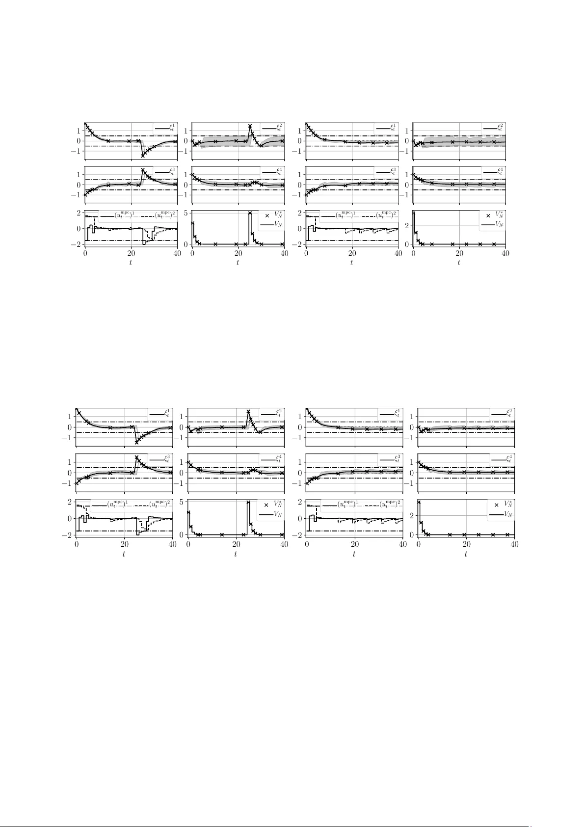
A Decen tralized Ev en t-Based Approac h for Robust Mo del Predictiv e Con trol ARMAN SHARIFI KOLARIJANI, SANDER C. BREGMAN, PEYMAN MOHAJERIN ESF AHANI, T AM ´ AS KEVICZKY Abstract. In this pap er, w e prop ose an even t-based sampling p olicy to implemen t a constraint-tigh tening, robust MPC method. The proposed p olicy enjoys a computationally tractable design and is applicable to perturb ed, linear time-inv ariant systems with polytopic constraints. In particular, the triggering mec hanism is suitable for plants with no centralized sensory no de as the triggering mechanism can b e ev aluated lo cally at each individual sensor. F rom a geometrical viewp oint, the mechanism is a sequence of h yp er-rectangles surrounding the optimal state tra jectory suc h that robust recursiv e feasibility and robust stabilit y are guaran- teed. The design of the triggering mechanism is cast as a constrained parametric-in-set optimization problem with the volume of the set as the ob jective function. Re-parameterized in terms of the set vertices, we show that the problem admits a finite tractable conv ex program reformulation and a linear program relaxation. Several n umerical examples are presented to demonstrate the effectiv eness and limitations of the theoretical results. 1. Introduction No wada ys, net work ed control systems (NCSs) generally demand an array of compatibility and efficiency measures from con trol design metho ds, such as utilization under shared resources, applicabilit y to mobile tasks, and compatibility with digital comm unication infrastructures [ 4 ]. Ev ent-based co n trol (EBC) is a class of strategies that aim to improv e efficiency of NCSs in the context of communication and computation. In EBC, the dynamics determine the instance to up date a control action (contrary to the traditional case where a control action is up dated p erio dic al ly ) [ 17 ]. There are tw o options to implement such an even t-based logic: embedded in the sensory system, the so-called event-trigger e d c ontr ol [ 36 ] and [ 15 ], or embedded in the controller, the so-called self-trigger e d c ontr ol [ 2 ] and [ 28 ]. The resp onsible en tity to determine an up date instance is known as the triggering me chanism . In particular, mo del predictiv e control (MPC) metho ds [ 11 ] ha ve b een the sub ject of many studies in order to b e amended with an EBC mindset. MPC methods are a class of on-line optimization-based con trol app roaches. In these metho ds, a measure of system performance is optimized o ver a finite horizon while states and inputs are sub ject to certain constraints. When the underlying dynamics is uncertain, the specific term r obust MPC (RMPC) is used for these methods in the literature [ 25 ]. W e refer the interested reader to the survey pap ers [ 27 ] and [ 26 ] that discuss ab out differen t asp ects of MPC. T raditionally , the con troller solv es the corresp onding optimization problem at every time step and produces as outcomes tw o sequences of optimal inputs and states. Then, the controller s ends the first elemen t of input sequence to the actuators and the remaining elements of the input sequence and the whole state sequence are discarded. These discarded predictions in a standard MPC setting can serv e as a basis to design a triggering mec hanism. Moreo ver, the computational burden of MPC methods is a ma jor dra wback, hindering their usage in practice. One thus hop es by employing an EBC approach to reduce the frequency at which the underlying optimization problem is solved. Notice that there are already some techniques in the MPC literature (the so-called warm start approaches [ 40 ]) that exploit the computed sequences at the previous step to speed up the computation pro cess. Date : September 24, 2019. The authors are with the Delft Center for Systems and Con trol, TU Delft, The Netherlands ( { a.sharifikolarijani,s.c.bregman,p.mohajerinesfahani,t.keviczky } @tudelft.nl ). 1 2 A. SHARIFI KOLARIJANI, S. C. BREGMAN , P . MOHAJERIN ESF AHANI, T. KEVICZKY There is also a big incentiv e to exploit the computed sequences of MPC metho ds in a class of NCSs, namely , wir eless sensor/actuator networks (WSANs). In these systems, the most imp ortan t concern is the energy efficiency , see e.g., [ 39 , Section IV.B]. The main source of energy depletion in a wireless no de is the transceiv er (resp onsible for sending and receiving data). T o reduce the frequency of data transfer, it is hence more efficient (energy-wise) to aggregate the data into a single pac ket (if p ossible) and transmit the resulting pac ket at once o ver the communication net work [ 22 ] and [ 24 ]. Statemen t of contribution: In this pap er, an ev ent-triggered (ET) approac h is prop osed to implement an RMPC metho d on p erturbed, linear time-inv ariant (L TI) systems. The RMPC metho d is originally in tro duced in [ 31 ]. The core idea b ehind the ET approach is to construct a sequence of hyp er-r e ctangles around the optimal state sequence av ailable from solving the RMPC problem. Then, these h yp er-rectangles will b e sent to the sensors. The optimal input sequence will also b e transmitted to the actuators. Once the observ ed states at the sensory units leav e these hyper-rectangles, a triggering happens and the states at the triggering instance will be transmitted to the co n troller. This pro cedure is then repeated in a sampled-data fashion. A key feature of the prop osed ET approach is its ability to decide based on the lo cal observ ation of eac h individual sensor, whether to trigger or not. This feature stems from the fact that the sets describing the triggering mec hanism are hyper-rectangles. Hence, the conditions required for a triggering in differen t states of the system are indep enden t of eac h other. This feature is in particular appealing to systems with de c entr alize d (spatially disp ersed) sensing units, including systems equipped with high-level (or supervisory) MPC metho ds, e.g., w ater treatment systems [ 35 ], HV A C systems [ 20 ], and commercial refrigeration systems [ 18 ] to name a few. Notice that the collo cation of the triggering mechanism and the sensory units is ph ysically imp ossible in suc h systems. Moreov er, the addition of a c entr al no de (on which the triggering mechanism is placed on) to collect the sensory data comes at the price of extra communication bandwidth usage. On the theoretical side, the design of the ET approach is de c ouple d from the design of the underlying RMPC metho d. As a result, a fair comparison b et w een the performances of the ET and standard implementations of the RMPC metho d b ecomes p ossible. This paper extends the results of the authors’ previous work in [ 9 ] in m ultiple directions, in particular, by simplifying the triggering “law”. The approach in [ 9 ] requires an “adv anced” triggering mec hanism that is resp onsible for (i) constructing certain input and state sequences, (ii) ev aluating the satisfaction of MPC’s constrain ts b y these sequences, and (iii) comparing the v alues of the cost function based on the constructed sequences with the v alue function at the last triggering instance. The main con tributions of the pap er are summarized as follows. • Decoupled recursive feasibilit y and stability: Given an RMPC metho d in place, we prop ose a set-theory-based, ET approach that preserves robust recursive feasibilit y and robust stabilit y . The prop osed approach is decoupled from the control syn thesis pro cess and do es not require additional assumptions, such as extra conditions on eigenv alues of weigh ting matrices in the cost function or the need to define user-sp ecified thresholds for the triggering mechanism (Theorem 4.1 ). • Decentralized applicability: The prop osed approach enjoys a decentralized triggering mechanism that only requires lo cal sensory information (Definition 3.3 ). • T ractable conv ex program reformulation: W e show that a certain type of non-con vex v olume- maximization problem with set-based constraints that is deplo y ed to design the triggering mechanism admits a finite tractable con vex program (CP) reform ulation (Theorem 4.4 ). • Sub optimal linear program relaxation: Motiv ated by an approach in the literature, we further sho w that a linear program (LP) relaxation of the CP reformulation is possible (Theorem 4.5 ). Literature review: In what follows, we first review several even t-triggered, MPC approac hes. W e then close this section b y giving a brief account of several computationally efficien t approac hes that are customized for MPC problems. R elate d works: Let us first mention the shared properties of the references b elow: linear discrete-time mo dels, ev ent-triggering mechanisms, constrained MPC metho ds, minimal (to none) coupling of the parameters of A DECENTRALIZED EVENT-BASED APPR OACH FOR ROBUST MODEL PREDICTIVE CONTROL 3 the triggering mec hanism and the considered MPC metho d, and a computationally viable approach to design the triggering mechanism. T o deal with practical issues such as a band-limited communication channel, a nov el design approac h for NCSs is prop osed in [ 16 ]. They emplo y the notion of moving horizon [ 30 ] to design the estimator and con- troller. A remark able character of their approac h is its ability to decide on-the-fly which input c hannel should b e up dated (i.e., a certain t yp e input-channel even t-triggering con trol). In case of collo cated controller and actuator units, an ev ent-based estimator with a b ounded cov ariance matrix is designed in [ 34 ]. While the estimator receives data via a Leb esgue sampling approach, it p eriodically up dates the con troller’s informa- tion regarding the disturbances with a p olytopic ov er-appro ximation of the co v ariance matrix. The authors of [ 7 ] prop ose an in teresting transmission strategy for wireless sensor/con troller communications with prac- tical energy-aw are provisions (the con troller is collocate d with the actuator system). Using some predefined thresholds for eac h state’s sensor (i.e., an ` 1 -t yp e triggering mec hanism), the con troller is computed offline using an explicit MPC approac h [ 6 ]. Based on a prescrib ed 2-norm ball around the optimal state tra jectory , the authors in [ 23 ] prop ose a triggering mechanism for WSANs. They show that the approach is robustly stable to a set that is a function of the radius of threshold ball and the maximal 2-norm of disturbance. F or linear, contin uous-time dynamical systems affected by a Wiener pro cess, a co-design metho d (i.e., si- m ultaneous design of the scheduler and the controller) is prop osed in [ 3 ]. The main idea is inspired by the notion of r ol lout from dynamic pr o gr amming [ 8 ]. More imp ortan tly , the authors sho w that under some mild conditions, an even t-based control approach outperforms a traditional con trol approach w.r.t. closed-lo op p erformance/a v erage transmission rate. (Notice that for most of the approaches in the literature including our paper such a guarantee is not provided.) A set theoretic triggering mec hanism is in tro duced in [ 10 ] for systems with collocated controller and sensory units. The approac h is inspired by the tub e-b ase d MPC pro- p osed in [ 29 ]. By exploiting the kno wn probability distribution of disturbance, they also guaran tee an av erage sampling rate. Ho wev er, their tube-contraction method requires a certain t ype of realization of a discrete-time system, see [ 10 , Remark 8]. Demirel et al., in tro duce a sensor/actuator ev en t-triggering mec hanism for control systems with limited num b er of control messages (i.e., communication and computation resources are scarce) [ 12 ]. They relax the underlying combinatorial problem in to a conv ex one b y an appropriate definition of ev ent thresholds. In [ 19 ], a pack etized approach is prop osed for input-affine, nonlinear systems with b ounded additiv e disturbances in contin uous-time. In the prop osed approac h, an RMPC controller (connected via a communication netw ork to the plant) takes into account the mismatched uncertainties while an integral sliding-mo de controller [ 37 ] (placed at the plant) counters the effect of the matched uncertain ties. A lgorithmic viewp oint: An MPC optimization problem is computationally exp ensiv e b y itself. Hence, the merit of an even t-based p olicy of implemen tation would b e lost if the mechanism demands a drastically higher computational effort compared to the underlying MPC problem. Dunn and Bertsek as in [ 13 ] exploit the structure of their problem to reduce the cubic complexity of computing a Newton ste p to a linear one. In [ 38 ], the authors use a sp ecific or dering of decision v ariables to promote a sparse structure that decreases the cost of computing a control action. The authors in [ 32 ] employ a simple, gradient-based algorithm to solv e an MPC problem while pro viding a priori computational complexity certificate. The lay out of the pap er is as follows. The mathematical notions used in the pap er are outlined in Sec- tion 2 . Section 3 is devoted to the considered RMPC method. The main results regarding the even t-based implemen tation p olicy are introduced in Section 4 . Section 5 contains the technical proofs. Several n umerical examples are presen ted in Section 6 to ev aluate the effectiveness and limitations of the theoretical results. Finally , we presen t several future researc h directions in Section 7 . 2. Not a tion and Preliminaries W e b egin with a brief review of the mathematical preliminaries employ ed in the rest of the paper. Notation: The set of non-negative integers is denoted b y Z ≥ 0 . Giv en p ositiv e integers m and n , R m and R m × n represen t the m -dimensional Euclidean space and the space of m × n matrices with real entries, 4 A. SHARIFI KOLARIJANI, S. C. BREGMAN , P . MOHAJERIN ESF AHANI, T. KEVICZKY resp ectiv ely . Given tw o integers i, j where i ≤ j , { i : j } := { i, i + 1 , . . . , j } . F or any pairs of vectors a, b ∈ R n , the inequality a < ( ≤ ) b is realized in a comp onen t-wise manner. Given a vector v ∈ R n and a scalar p ≥ 1, k v k p denotes the p -norm  P n i =1 ( v i ) p  1 /p . Giv en a matrix M ∈ R m × n , M ij denotes the i -th row, j -th column entry of M . Moreo ver, the matrix M + ∈ R m × n is the matrix with entries M + ij := max { 0 , M ij } . The n × n zero and iden tity matrices are denoted by 0 n and I n , resp ectiv ely . Giv en a set S ⊂ R n and a matrix M ∈ R m × n , the set M S denotes the set { c ∈ R m : ∃ s ∈ S , M s = c } . Giv en a matrix M  0 (i.e., p ositiv e definite), the squared weigh ted distance of a p oin t r ∈ R n from a closed set S ⊂ R n is defined as d M ( r , S ) := min s ∈S || r − s || 2 M = min s ∈S ( r − s ) > M ( r − s ). Denote the pro jection of r on to S b y Π M ( r , S ) ∈ argmin s ∈S d M ( r , S ). Note that when S is also conv ex, the pro jection is unique. Given sets C and D , the Pon try agin difference C  D and the Mink o wski sum C ⊕ D are defined as C  D := { c : c + d ∈ C , ∀ d ∈ D } and C ⊕ D := { c + d : ∀ c ∈ C , ∀ d ∈ D } , respectively . The function sign( · ) represen ts the standard sign function. Giv en a set X ∈ R n and an extende d real-v alued function f : X → [ −∞ , + ∞ ], the effe ctive domain of f is the set dom( f ) = { x ∈ X : f ( x ) < ∞} . The following result will b e used frequently in the developmen t of the triggering mechanism. Lemma 2.1 (Set-difference low er b ound [ 31 ]) . L et r b e a ve ctor in R n , B and C b e two c omp act sets in R n , and M b e a p ositive definite matrix in R n × n . Then, d M ( r + c, B ) ≤ d M ( r , B  C ) , for al l c ∈ C . W e now revisit some notions from conv ex analysis (see e.g., [ 21 , Section 2] for a compact exposition of the sub ject). Given a set S ⊂ R n , the supp ort function of S ev aluated at η ∈ R n is h S ( η ) := sup s ∈S h η , s i . The domain K S on which the support function is defined is a con vex cone pointed at the origin. If S is b ounded, then K S := R n . Given a matrix M ∈ R n × m and a vector v ∈ R n , if M > v ∈ K S , then h M S ( v ) := h S ( M > v ). Supp ose S ⊂ R n is closed and con vex. Then, S := { s ∈ R n : h η , s i ≤ h S ( η ) , ∀ η ∈ K S } , i.e., the intersection of its supp orting halfplanes. A set S ⊂ R n is called a p olyhedron, if S = { s ∈ R n : A S s ≤ b S } , A S ∈ R m × n , b S ∈ R m . If the p olyhedron S is b ounded, the set is called a p olytop e and its representation given ab o ve is kno wn as the H-r epr esentation . F urthermore, the supp ort function h S ( η ) of a polytop e S is the solution of the LP , h S ( η ) = max s h η , s i sub ject to A S s ≤ b S . Given the H -representation of a p olytop e, we employ the notations a i, S ∈ R 1 × n and a S ,j ∈ R m × 1 to denote the i -th ro w and the j -th column of A S , resp ectiv ely . Moreo ver, b i, S is the i -th entry of b S . Giv en a p olyhedron S ⊂ R n and a set V ⊂ R n , assume that h V ( a > i, S ) is well-defined for all i ∈ { 1 : m } . Then, S  V :=  z ∈ R n : h a > i, S , z i ≤ b i, S − h V ( a > i, S ) , ∀ i ∈ { 1 : m }  . F or an y vector-pairs l, u ∈ R n suc h that l < u , the full-dimensional con vex p olytop e B ( l , u ) := { x ∈ R n : l ≤ x ≤ u } = { x ∈ R n : A B x ≤ b B } is called a hyp er-r e ctangle , where A B := [ I n − I n ] > and b B = [ u > − l > ] > . 3. Robust model Predictive Control Method In this section, w e introduce the class of constrained dynamical systems considered in this pap er, follow ed b y the description of the RMPC metho d. A t last, we formally state the problem addressed in this pap er. Consider an L TI system with a b ounded additive disturbance given by x + = Ax + B u + w, (1) where x + is the successor state and x , u , and w are the current state, input and disturbance, resp ectively . The current state, input, and disturbance are sub ject to the hard constrain ts x ∈ X ⊂ R n x , u ∈ U ⊂ R n u , w ∈ W ⊂ R n x . (2) A system is called the nominal system asso ciated with ( 1 ) when w = 0. Given a p ositiv e integer N , let U := U N = Q N − 1 i =0 U ( W := W N ) denote the class of admissible control sequences u := { u i } i ∈{ 0: N − 1 } (admissible disturbance sequences w := { w i } i ∈{ 0: N − 1 } ). Initiated at state x , the solution to ( 1 ) at time i with the control and disturbance sequences u and w , resp ectiv ely , is denoted by φ u , w i ( x ). Similarly , we define φ u , w ( x ) := { φ u , w i ( x ) } i ∈{ 0: N } . Moreo ver, let φ u , 0 i ( x ) denote the nominal solution with the input sequence u initiated at state x . The RMPC metho d is designed suc h that the state x and the input u ev entually con verge A DECENTRALIZED EVENT-BASED APPR OACH FOR ROBUST MODEL PREDICTIVE CONTROL 5 to some user-defined tar get sets T X ⊂ R n x and T U ⊂ R n u , resp ectively , while the constraints ( 2 ) are satisfied at all times. Assumption 3.1 (System & constraint sets) . (i) Nominal c ontr ol lability: The p air ( A, B ) is c ontr ol lable. (ii) Polytopic sets: The sets X , U , T X , T U , and W ar e al l c onvex, c omp act p olytop es c ontaining their underlying sp ac es’ origin in their interior. W e start with introducing tw o types of feedback gains which are used in the RMPC metho d and are essen tial for the construction of the triggering mec hanism. Let F ∈ R n × m b e a giv en feedback gain that guaran tees the stability of the nominal system with u = F x . The nominal gain F can b e designed so that a satisfactory p erformance (e.g., in an LQ optimal con trol sense) is guaranteed for the nominal system. Let in teger N ≥ n x + 1 b e the horizon length of the RMPC metho d and integer M b e given, where M ∈ { n x : N − 1 } . Supp ose next that a set of feedback gains K = { K i } i ∈{ 0: N − 1 } are given suc h that Q M i =1 ( A + B K i ) = 0, i.e., for all k ≥ M , φ u , 0 k ( x ) = 0. W e call the set of gains K the tightening gains since these gains are employ ed in the state and input constraint tightening pro cess. W e refer the interested reader to [ 31 , Section IV] for a p ossible approach to construct the gains K . The constraint tightening approac h is applied to the input, state, input target, and state target sets, that is, for all i ∈ { 0 : N − 2 } , U 0 = U , U i +1 = U i  K i L i W , (3a) X 0 = X , X i +1 = X i  L i W , (3b) T U 0 = T U , T U i +1 = T U i  K i L i W , (3c) T X 0 = T X , T X i +1 = T X i  L i W , (3d) where L 0 = I n x and L i +1 = ( A + B K i ) L i for all i ∈ { 0 : N − 2 } . Notice that the M -step nilp otency of the set of gains K implies that for all i ∈ { M : N − 1 } , L i = 0 n x . Let the terminal set X f ⊂ R n x b e a c ontr ol invariant set for the nominal system, i.e., ( A + B F ) ξ ∈ X f for all ξ ∈ X f . Assumption 3.2 (T erminal set) . F or al l ζ ∈ X f , the fol lowing c onditions hold: ζ ∈ X N − 1 ∩ T X N − 1 , F ζ ∈ U N − 1 ∩ T U N − 1 . F or the sak e of notational simplicity , let us define U N := Q N − 1 i =0 U i and X N := Q N − 1 i =0 X i × X f . The c ost function of the RMPC problem is V N ( x, u ) := N − 1 X i =0 d Q ( φ u , 0 i ( x ) , T X i ) + d R ( u i , T U i ) + δ feas  u , φ u , 0 ( x )  , (4) where δ feas  u , φ u , 0 ( x )  = 0 if u ∈ U N and φ u , 0 ( x ) ∈ X N , and = ∞ otherwise, is the indic ator function of the set U N × X N . Notice that the input and state constraints are embedded in the ob jective function via the indicator function. The optimization problem for a finite horizon N with an initial state x reads as V ∗ N ( x ) := min u V N ( x, u ) , (5) with u mpc ( x ) := argmin u V N ( x, u ) as the optimal input sequence. When it is clear from the context, we ma y instead use the shorthand notation u mpc . The abov e sequence of inputs is indeed an optimal solution to a nominal (i.e., w = 0 ) finite optimization problem emerging in the con text of finite horizon MPC in the rest of the pap er. In this ligh t, we denote this nominally optimal controller b y a similar lab el, for whic h the asso ciated nominal state sequence is φ u mpc , 0 ( x ). In a standard RMPC setting, the optimal con trol problem ( 5 ) is solved. The first element u mpc 0 ( x ) of u mpc ( x ) is then applied to the plan t yielding to the closed-loop dynamics x + = Ax + B u mpc 0 ( x ) + w . In an even t-based setting, the triggering mechanism generally exploits the optimal state sequence φ u mpc , 0 ( x ) in order to p ossibly employ the rest of elements in the nominally optimal input v ector u mpc ( x ). The challenge 6 A. SHARIFI KOLARIJANI, S. C. BREGMAN , P . MOHAJERIN ESF AHANI, T. KEVICZKY in designing the triggering mechanism is then to guarantee robust stability and robust recursive feasibilit y of the resulting even t-triggered, closed-lo op dynamics. Definition 3.3 (T riggering mec hanism) . Given an initial state x and a se quenc e of (p ossibly) state-dep endent, hyp er-r e ctangular sets E ( x ) := E 0 ∪ {E i ( x ) } N − 1 i =1 ⊂ ( R n x ) N , the triggering instanc e is define d by k w trig ( x ) := min  j ∈ { 0 : N − 1 } : φ u mp c , w j ( x ) − φ u mp c , 0 j ( x ) / ∈ E j ( x )  , (6) wher e E 0 := R n x . The quantit y k w trig ( x ) is known as the inter-exe cution time in the literature. One can observe that φ u mpc , w 0 ( x ) = φ u mpc , 0 0 ( x ) = x . As a result, φ u mpc , w 0 ( x ) − φ u mpc , 0 0 ( x ) = 0 ∈ R n x = E 0 , and th us k w trig ( x ) ≥ 1. The closed-lo op dynamics is then, for all t ∈ Z ≥ 0 , ξ t +1 = Aξ t + B u mpc t − τ t ( ξ τ t ) + w t , (7a) τ t +1 = ( τ t , t − τ t ≤ N − 1 and ξ t − φ u mpc , 0 t − τ t ( ξ τ t ) ∈ E t − τ t ( ξ τ t ) , t, otherwise , (7b) giv en the initial state ξ 0 and the initial triggering instance τ 0 = 0. Here, τ t denotes the last triggering instance up to time t . Also, notice that a mandatory triggering is put in place at time τ t + N . The problem addressed in this pap er is now introduced. Problem 3.4. Consider the close d-lo op dynamics ( 7 ) under Assumptions 3.1 - 3.2 . Devise an appr o ach to c onstruct the se quenc e of triggering sets E ( ξ τ t ) in ( 6 ) such that the tr aje ctories of the close d-lo op dynamics satisfy: • Recursive feasibilit y: If V ∗ N ( ξ 0 ) < ∞ , then V ∗ N ( ξ t ) < ∞ , for al l t ∈ Z ≥ 0 ; • Robust stabilit y: The states and inputs of the close d-lo op dynamics c onver ge to the tar get sets T X and T U , r esp e ctively ( lim t →∞ V ∗ N ( ξ t ) = 0 ). Remark 3.5 (Smart actuators and sensors) . The actuator and sensor units ar e “smart” in the fol lowing sense. The actuator (sensor) units c an buffer the time-stamp e d and p acketize d se quenc e u mp c ( ξ τ t ) ( { φ u mp c , 0 s ( ξ τ t ) ⊕ E s ( ξ τ t ) } N − 1 s =1 ). The actuator units c onse cutively apply t he input action u mp c s − τ t ( ξ τ t ) on the plant at e ach time s ∈ { τ t : τ t +1 − 1 } . The sensor units evaluate the triggering c ondition ξ s / ∈ φ u mp c , 0 s − τ t ( ξ τ t ) ⊕ E s − τ t ( ξ τ t ) , at e ach time s ∈ { τ t + 1 : τ t + N − 1 } . When the triggering c ondition holds at some time s , the sensors send the most r e c ent states ξ s to the c ontr ol ler and the triggering instanc e is set to τ t +1 = s . Remark 3.6 (Iteration Complexit y) . RMPC pr oblems with line ar dynamics, a quadr atic c ost function, and p olytopic c onstr aints ar e quadratic programs for which de dic ate d solvers pr ovide the c omplexity p er iter ation O ( N ( n x + n u ) 3 ) [ 38 ] . 4. Main Resul ts In this section, w e provide sev eral approaches to construct the sequence of sets E ( x ) whic h meets the requiremen ts of Problem 3.4 . T o this end, we begin with describing a certain t yp e of constrained optimization problem that pro duces E ( x ). Based on these constructed sets, we then state the main theoretical results of this pap er. 4.1. Construction of Hyp er-Rectangles Let j ∈ { 1 : N − 1 } . The pro cedure to construct each hyper-rectangle E j ( x ) comprises the parametric represen tation of E j ( x ), the definition of auxiliary quantities asso ciated with E j ( x ), and finally the optimization problem to find E j ( x ). A DECENTRALIZED EVENT-BASED APPR OACH FOR ROBUST MODEL PREDICTIVE CONTROL 7 Notice that one wa y to represent a hyper-rectangle E j ( x ) is E j ( x ) :=   ∈ R n x : − e j ( x ) ≤  ≤ e j ( x )  , for some vectors e j ( x ) , e j ( x ) ∈ R n x ≥ 0 . In other words, each hyper-rectangle E j ( x ) is parameterized by 2 n x en tries of e j ( x ) and e j ( x ). Let us now introduce the auxiliary quantities inv olved in the deriv ation of E j ( x ). Let A cl := ( A + B F ) b e the nominal, closed-lo op state matrix. Define the input sequence ˜ u ( x ; j ) and the asso ciated state se- quence φ ˜ u , 0 ( x ; j ) as ˜ u i ( x ; j ) := ( u mpc j + i ( x ) , i ∈ { 0 : N − j − 1 } , F A j + i − N cl φ u mpc , 0 N ( x ) , i ∈ { N − j : N − 1 } , (8a) φ ˜ u , 0 i ( x ; j ) :=    φ u mpc , 0 j + i ( x ) , i ∈ { 0 : N − j } , A j + i − N cl φ u mpc , 0 N ( x ) , i ∈ { N − j + 1 : N } . (8b) Notice that the ab o ve c andidate input se quenc e is constructed by concatenating the last N − j elements of u mpc ( x ) with the nominal feedbac k F (recursiv ely) applied to the optimal terminal state φ u mpc , 0 N ( x ). Define T U N := Q N − 1 i =0 T U i and T X N := Q N − 1 i =0 T X i . Denote now the pro jections of optimal state and input sequences φ u mpc , 0 ( x ) and u mpc ( x ) onto their corresponding target sets by s X ( x ) ∈ T X N and s U ( x ) ∈ T U N , where for all i ∈ { 0 : N − 1 } , s X i ( x ) := Π Q ( φ u mpc , 0 i ( x ) , T X i ) , s U i ( x ) := Π R ( u mpc i ( x ) , T U i ) . Based on the ab o ve definition, the next tw o auxiliary quantities are defined as follows. Let ˜ s U ( x ; j ) and ˜ s X ( x ; j ) represent the pro jection of ˜ u ( x ; j ) and φ ˜ u , 0 ( x ; j ) onto T U N and T X N , resp ectively . W e hav e ˜ s U i ( x ; j ) := ( s U j + i ( x ) , i ∈ { 0 : N − j − 1 } , ˜ u i + j ( x ; j ) , i ∈ { N − j : N − 1 } , (9a) ˜ s X i ( x ; j ) := ( s X j + i ( x ) , i ∈ { 0 : N − j } , φ ˜ u , 0 j + i ( x ; j ) , i ∈ { N − j + 1 : N − 1 } . (9b) Let us clarify the conv en tions used in ( 9 ). Notice that the definition of ˜ u i ( x ; j ) in ( 8a ) implies that ˜ u i ( x ; j ) ∈ T U N − 1 ⊆ T U i , for all i ∈ { N − j : N − 1 } . That is, the distance d R ( ˜ u i ( x ; j ) , T U i ) = 0, and hence, Π R ( ˜ u i ( x ; j ) , T U i ) = ˜ u i ( x ; j ), as giv en in ( 9a ). A similar line of reasoning has b een used in ( 9b ). W e next adopt the feedback gains ˜ K i and the state-transition matrices ˜ L i defined as ˜ K 0 = 0 n u × n x , ˜ K i +1 = K i , ∀ i ∈ { 0 : N − 2 } , (10a) ˜ L 0 = I n x , ˜ L i +1 = ( A + B ˜ K i ) ˜ L i , ∀ i ∈ { 0 : N − 1 } . (10b) In the follo wing, w e use the matrices ( 10 ) to iden tify certain sets around the optimal state sequence φ u mpc , 0 ( x ). These sets in turn will b e used to formulate recursive feasibility and robust stability for the even t-triggering setting (see the problem ( 12 ) and Section 5.1 ). Let us now provide tw o definitions for the v olume of E j ( x ), that are v ol 1 ( E j ( x )) := Y p ∈{ 1: n x }  e p j ( x ) + e p j ( x )  , (11a) v ol 2 ( E j ( x )) := Y p ∈{ 1: n x }  e p j ( x ) × e p j ( x )  , (11b) where e p j ( x ) (res p. e p j ( x )) denotes the p -th entry of e j ( x ) (res p. e j ( x )). Notice that ( 11a ) is the standard definition of v olume for E j ( x ) in R n x . As it will b e discussed later on, the application of ( 11a ) to construct E j ( x ) leads to a more asymmetric spread of E j ( x ) around φ u mpc , 0 j ( x ) compared to the application of ( 11b ). 8 A. SHARIFI KOLARIJANI, S. C. BREGMAN , P . MOHAJERIN ESF AHANI, T. KEVICZKY The asymmetry in turn implies that the triggering mec hanism has no robustness in certain error directions, see Remark 4.7 for further details. Nonetheless, the definition ( 11a ) leads to the construction of sets that ha ve the maximum p ossible volume, in particular, higher than the ones constructed based on ( 11b ). F or all j ∈ { 1 : N − 1 } , the problem to find each E j ( x ) is max e j ( x ) ,e j ( x ) ≥ 0 v ol q ( E j ( x )) (12a) s.t. φ ˜ u , 0 i ( x ; j ) ∈ X i  ˜ L i E j ( x ) , ∀ i ∈ { 0 : N − 1 } , (12b) ˜ u i ( x ; j ) ∈ U i  ˜ K i ˜ L i E j ( x ) , ∀ i ∈ { 0 : N − 1 } , (12c) ˜ s X i ( x ; j ) ∈ T X i  ˜ L i E j ( x ) , ∀ i ∈ { 0 : N − 1 } , (12d) ˜ s U i ( x ; j ) ∈ T U i  ˜ K i ˜ L i E j ( x ) , ∀ i ∈ { 0 : N − 1 } , (12e) where q ∈ { 1 , 2 } determines which t yp e of the volume definition in ( 11 ) is chosen. Notice that the ob jective function vol q ( E j ( x )) is a nonlinear, non-conv ex function with a decision v ariable E j ( x ). Hence, the prob- lem ( 12 ) is difficult to solv e. In the next subsection, we show that this problem remains practically solv able, in particular, the set-based constraints ( 12b )-( 12e ) are effectively representable by linear inequalities (i.e., p olytopic inequalities) suc h that (i) the optimization problem ( 12 ) has a CP counterpart (in Theorem 4.4 ), and (ii) the optimization problem ( 12 ) admits an LP relaxation (in Theorem 4.5 ). 4.2. Ev ent-Based Implemen tation W e first show that robust s tabilit y of the even t-triggered, closed-lo op dynamics ( 7 ) is guaran teed, whic h in turn leads to recursiv e feasibilit y of the closed-lo op system. The triggering mechanism ( 6 ) is constructed b y the approach prop osed in ( 12 ). W e next establish that the non-conv ex problem ( 12 ) to construct the h yp er-rectangles E ( x ) has a CP reformulation and an LP relaxation, and therefore can b e efficien tly solved in practice. Theorem 4.1 (Robust conv ergence) . Consider the close d-lo op dynamics ( 7 ) , and supp ose that the initial state ξ 0 is fe asible (i.e., V ∗ N ( ξ 0 ) < ∞ ). F or al l s ∈ { τ t + 1 : τ t +1 } , ther e exists an input se quenc e u ∈ U N such that V ∗ N ( ξ τ t +1 ) − V ∗ N ( ξ τ t ) ≤ V N  ξ s , u ( ξ s )  − V ∗ N ( ξ τ t ) ≤ −  s − τ t − 1 X k =0 d Q ( φ u mp c , 0 k ( ξ τ t ) , T X k ) + d R ( u mp c k ( ξ τ t ) , T U k )  . (13) In p articular, the close d-lo op dynamics ( 7 ) is asymptotic al ly stable, i.e., lim t →∞ V ∗ N ( ξ t ) = 0 . Remark 4.2 (Recursiv e feasibilit y) . Notic e that the se c ond ine quality in ( 13 ) implies that V N  ξ s , u ( ξ s )  < ∞ , for al l s ∈ { τ t + 1 : τ t +1 } . In other wor ds, the optimization pr oblem ( 5 ) r emains fe asible for al l time t ∈ Z > 0 . Remark 4.3 (T ransmission proto col) . We assume that al l sensor and actuator units ar e clo ck-synchr onize d. When the pr oblem ( 5 ) is solve d, the c ontr ol ler no de sends: (i) u mp c ( ξ τ t ) to the actuator no des and (ii) e ach entry of φ u mp c , 0 j ( ξ τ t ) − e j ( ξ τ t ) and φ u mp c , 0 j ( ξ τ t ) + e j ( ξ τ t ) to the c orr esp onding sensory no des, for al l j ∈ { 1 : N − 1 } . Mor e over, the n x sensor units de clar e a triggering instanc e to e ach other, thr ough a c ost-efficient short-r ange tr ansmission. Then, al l sensors de clar e their time-stamp e d, observe d states to the c ontr ol ler. The successful usage of the ab o ve results is conditioned up on the premise that there exist computationally tractable metho ds to construct the sets E ( x ). W e now revisit problem ( 12 ) to show that such a premise is v alid by providing t wo frameworks: one in a CP form and another one in an LP form. In these framew orks, the parametric-in-set constraints ( 12b )-( 12e ) can be reformulated in to a new set of linear inequalities in terms of the vertices of each set E j ( x ). W e shall call the p olytope represented by the derived linear inequalities, the A DECENTRALIZED EVENT-BASED APPR OACH FOR ROBUST MODEL PREDICTIVE CONTROL 9 princip al p olytop e ¯ S . Both framew orks try to find a maximum-v olume hyper-rectangle E j ( x ) inscrib ed (or con tained) in the principal polytop e suc h that 0 ∈ E j ( x ). In the LP framew ork, we partly emplo y some results from [ 5 ], see Section 5.2 and av oid reiterating the pro ofs of b orro wed material. F or notational conv enience, let ξ ∈ S  M B ( l , u ) represen t a concatenated version of the constrain t ( 12b )-( 12e ) where, in particular, B ( l, u ) := E j ( x ). Hereafter, when w e tak e v olume (of a hyper-rectangle) as defined in ( 11 ) with index q = 1 and q = 2 referring to ( 11a ) and ( 11b ), resp ectiv ely . Theorem 4.4 (V olume maximization - CP reformulation) . Consider a ve ctor ξ ∈ R p , a matrix M ∈ R p × k , and a p olytop e S = { s ∈ R p : A S s ≤ b S } c ontaining the origin wher e A S ∈ R m × p and b S ∈ R m . The maximum volume hyp er-r e ctangle B ( l, u ) ⊂ R k that c ontains the origin and satisfies ξ ∈ S  M B ( l, u ) is B ( − v ∗ , v ∗ ) wher e v ∗ and v ∗ ar e the optimal solutions of the pr oblem (14) min v ,v f q  v , v  s.t. h w i , [ v > v > ] > i ≤ b i, S − a i, S ξ , ∀ i ∈ { 1 : m } , v ≥ 0 , v ≥ 0 , wher e for q ∈ { 1 , 2 } f 1  v , v  := − Σ j ∈{ 1: k } log  v j + v j ) , (15a) f 2  v , v  := − Σ j ∈{ 1: k } log  v j  + log  v j ) , (15b) and for al l j ∈ { 1 : k } w i j = (  M > a > i, S  j , if ˆ w i j = 1 , 0 , otherwise , (16a) w i k + j = ( −  M > a > i, S  j , if ˆ w i j = − 1 , 0 , otherwise , (16b) with ˆ w i := sign( M > a > i, S ) , for al l i ∈ { 1 : m } . Theorem 4.5 (V olume maximization - LP relaxation) . Supp ose the hyp otheses in The or em 4.4 hold. • ( q = 1 ) The maximum volume r -c onstr aine d hyp er-r e ctangle B ( l, u ) ⊂ R k that c ontains the origin and satisfies ξ ∈ S  M B ( l , u ) is B ( z ∗ , z ∗ + λ ∗ r ) for which z ∗ ∈ R k and λ ∗ ∈ R ar e the optimal solution of the pr oblem (17a) max z ,λ λ s.t. A S M z + ( A S M ) + r λ ≤ b S − A S ξ z + λr ≥ 0 , z ≤ 0 , wher e the j -th entry of r , j ∈ { 1 : k } , is define d as (17b) r j ( ¯ S ) := max z ,ω ω s.t. A S M z ≤ b S − A S ξ A S M ( z + ω e j ) ≤ b S − A S ξ z + ω e j ≥ 0 , z ≤ 0 , wher e e j ∈ R k is the unit ve ctor in the j -th dir e ction and the p olytop e ¯ S is ¯ S := { z ∈ R k : A S M z ≤ b S − A S ξ } . 10 A. SHARIFI KOLARIJANI, S. C. BREGMAN , P . MOHAJERIN ESF AHANI, T. KEVICZKY • ( q = 2 ) The maximum volume r -c onstr aine d hyp er-r e ctangle B ( l, u ) ⊂ R k that c ontains the origin and satisfies ξ ∈ S  M B ( l , u ) is B ( − λ ∗ r 1 , λ ∗ r 2 ) for which λ ∗ ∈ R is the optimal solution of the pr oblem (18a) max λ λ s.t. ( W ) + r λ ≤ B , wher e r =  r > 2 , r > 1  > and the j -th entry of r , j ∈ { 1 : 2 k } , is define d as (18b) r j := max ω ω s.t. W 0 ( ω e j ) ≤ B 0 , wher e e j ∈ R 2 k is the unit ve ctor in the j -th dir e ction, W =  w 1 , · · · , w m  > , W 0 =    W − I k 0 k × 1 0 k × 1 − I k    , B = b S − A S ξ , B 0 =  B > , 0 1 × 2 k  > , and for al l i ∈ { 1 : m } , w i ar e define d in ( 16 ) . W e should emphasize that although Theorems 4.4 & 4.5 pro vide a w ay to construct E j ( x ) with a maximal v olume, the derived set is not unique (the corresp onding cost functions of these approac hes are not strictly con vex to guarantee the uniqueness of solution). In the remainder of the pap er, we denote the construction approac h based on the CP ( 14 ) with q = 1 and q = 2 by CP 1 and CP 2 , resp ectiv ely . F urthermore, LP 1 represen ts the LP relaxation ( 17 ) of CP 1 and LP 2 denotes the LP relaxation ( 18 ) of CP 2 . 4.3. F urther Comments on Complexity and Sensitivity In the rest of this section, we allude briefly to t wo important practical aspects of the prop osed construction approac hes and p ossible directions to improv e them. First, since these approaches are implemen ted online, they require an extra computation step b esides the computation of the optimal input sequence. Notice that fixed-thresholding approaches in the literature, for example [ 23 ], av oid this extra step by considering pre-defined triggering sets. W e pro vide the arithmetic complexity of the prop osed approaches to quantify the extra computational burden. T o this end, w e adopt the follo wing notion of an oracle to represent the optimization problems in this pap er. Let A ∈ R n c × n d , b ∈ R n c , c ∈ R n d , and f : R n d → R b e a concav e function. Also, let lp ( n c , n d ) denote the oracle complexit y for solving max η { c > η : Aη ≤ b } , and cp ( n c , n d ) denote the oracle complexity for solving max η { f ( η ) : Aη ≤ b } . Remark 4.6 (Computational complexity) . The or acle c omplexity of the CP r eformulations ( 14 ) in The o- r em 4.4 is cp ( m + 2 k , 2 k ) and of the LP r eformulations ( 17 ) and ( 18 ) in The or em 4.5 ar e lp ( m + 2 k , k + 1) + k × lp (2 m + 2 k , k + 1) and lp ( m, 1) + 2 k × lp ( m + 2 k , 1) , r esp e ctively. A p ossible r eme dy to cir cumvent these c omputations is to intr o duc e a state-indep enden t triggering law, as opp ose d to the curr ent state-dep endent law ( 6 ) . This extension would al low to c ompute the desir e d sets offline and only onc e. The other issue regarding the prop osed approaches is the asymmetry of the triggering sets with respect to the optimal state sequence. Let p olytop e S ⊂ R n x represen t the constrain ts ( 12b )-( 12e ) that the triggering set E j ( x ) satisfies. In other words, E j ( x ) is constructed inside S . Recall that E j ( x ) represents the “allow able” prediction error so that the triggering mechanism is not activ ated. Qualitativ ely sp eaking, for a “b etter” directional resilience against prediction errors, one would prefer symmetry in the constructed E j ( x ). The ab o v e statements are sc hematically depicted in Figure 1 . When S is well-shaped as in Figure 1(a) , the approac hes in Theorems 4.4 & 4.5 lead to a relatively symmetric set E j ( x ) with resp ect to the origin. When S is ill-shap ed as in Figure 1(b) , the constructed set E j ( x ) is how ev er extremely asymmetric with resp ect to the origin along some co ordinates. This difference is well-captured by the geometric measure r c r ◦ of S , where r c is A DECENTRALIZED EVENT-BASED APPR OACH FOR ROBUST MODEL PREDICTIVE CONTROL 11 − 2 − 1 0 1 2 x 1 − 1 . 5 − 1 . 0 − 0 . 5 0 . 0 0 . 5 1 . 0 1 . 5 2 . 0 x 2 E j ( x ) CP 1 E j ( x ) CP 2 E j ( x ) LP 1 E j ( x ) LP 2 ¯ S B 2 c B 2 ◦ (a) W ell-shaped p olytope example, r c r ◦ = 1 . 0861. − 2 − 1 0 1 2 x 1 − 3 . 0 − 2 . 5 − 2 . 0 − 1 . 5 − 1 . 0 − 0 . 5 0 . 0 0 . 5 x 2 E j ( x ) CP 1 E j ( x ) CP 2 E j ( x ) LP 1 E j ( x ) LP 2 ¯ S B 2 c B 2 ◦ (b) Ill-shap ed p olytope example, r c r ◦ = 8 . 0669. Figure 1. Comparison of the CP and LP approaches to construct E j ( x ) ⊆ S . (a) S is distributed in a fairly uniform manner around the origin. All the approaches provide close b eha viors. (b) S is distributed in a relatively uneven manner around the origin. The ap- proac hes CP 2 and LP 2 promote more symmetric constructions compared to the approaches CP 1 and LP 1 . the radius of the maximal 2-norm ball inside S , and r ◦ is the radius of the maximal 2-norm ball, centered at the origin and inside S . By definition, we hav e r c r ◦ ≥ 1. Observe that in well-shaped cas es r c /r ◦ ≈ 1 and in ill-shap ed cases r c /r ◦  1. Remark 4.7 (Directional sensitivity to prediction errors) . The dir e ctional sensitivity issue is the main r e ason for intr o ducing the se c ond definition ( 11b ) of the volume. T o se e this, assume first that our go al is to maximize the log value of the volume of E j ( x ) . Notic e that the first definition ( 11a ) solely aims for maximizing the width of E j ( x ) within S along e ach c o or dinate. On the other hand, the se c ond definition ( 11b ) maximizes the width of E j ( x ) in b oth p ositive and ne gative dir e ctions along e ach c o or dinate. As shown in Figur e 1 , in b oth c ases the set E j ( x ) c onstructe d by the appr o aches CP 2 and LP 2 is typic al ly mor e symmetric c omp ar e d to those c onstructe d by the appr o aches CP 1 and LP 1 . An inter esting r ese ar ch dir e ction to al leviate this sensitivity issue is to investigate the imp act of the MPC design p ar ameters (e.g., the tightening gains K or the tar get sets T X and T U ). 5. Technical Proofs 5.1. Pro of of Theorem 4.1 The pro of consists of five main steps. Each step is lab eled by the guaranteed prop erty . Let x := ξ τ t b e the state at the last triggering instance. Define the prediction error e w j ( x ) = φ u mpc , w j ( x ) − φ u mpc , 0 j ( x ) , (19) indicating the mismatch b et ween the p erturbed system and the nominal one. F or some in teger j ∈ { 0 : N − 1 } , supp ose that the mechanism is enabled at time j + 1, that is, either (1) j < N − 1 so that for all i ∈ { 0 : j } , e w i ( x ) ∈ E i ( x ) and e w j +1 ( x ) / ∈ E j +1 ( x ), or (2) j = N − 1 (see equation ( 7b )). W e omit the arguments of v ariables for con venience when it is clear from the context (unless mentioned otherwise). In what follows, we also use the notation ` ( x i , u i ) for d Q ( x i , T X i ) + d R ( u i , T U i ) for notational simplicity . 1) Inter-ev en t recursiv e feasibility: Define the c andidate input sequence u c ( x ; j ) such that for all i ∈ { 0 : N − 1 } , u c i := ˜ u i + ˜ K i ˜ L i e w j , (20a) 12 A. SHARIFI KOLARIJANI, S. C. BREGMAN , P . MOHAJERIN ESF AHANI, T. KEVICZKY and its asso ciated c andidate state sequence φ u c , 0 ( x ; j ), where for all i ∈ { 0 : N } , φ u c , 0 i := φ ˜ u , 0 i + ˜ L i e w j . (20b) Note that φ u c , 0 0 = φ u mpc , w j and u c 0 = u mpc j . W e no w establish that the sequences u c and φ u c , 0 satisfy u c ∈ U N and φ u c , 0 ∈ X N , i.e., V N ( φ u mpc , w j , u c ) < ∞ . By assumption, e w j ∈ E j . Moreov er, E j satisfies ( 12b )-( 12c ). F rom the definition of the P ontry agin difference, it follows that u c i ∈ U i and φ u c , 0 i ∈ X i , for all i ∈ { 0 : N − 1 } . Recall that L N − 1 = 0. Hence, ˜ L N = 0 and φ u c , 0 N = φ ˜ u , 0 N . F rom ( 8b ), we hav e φ ˜ u , 0 N = A j cl φ u mpc , 0 N ( x ). Since X f is a control inv arian t set, φ u c , 0 N ∈ X f . W e conclude that V N ( φ u mpc , w j , u c ) < ∞ . 2) Inter-ev en t cost function decay: Observe that d Q ( φ u c , 0 i , T X i ) = d Q ( φ ˜ u , 0 i + ˜ L i e w j , T X i ) ≤ d Q ( φ ˜ u , 0 i , T X i  ˜ L i E j ) , where w e made use of the definition ( 20b ) and Lemma 2.1 , respectively . Recall from ( 12d ) that ˜ s X i ∈ T X i  ˜ L i E j . Hence, 0 ≤ d Q ( φ u c , 0 i , T X i ) ≤ d Q ( φ ˜ u , 0 i , ˜ s X i ) . (21a) Similarly , one can arrive at 0 ≤ d R ( u c i , T U i ) ≤ d R ( ˜ u i , ˜ s U i ) . (21b) Consider i ∈ { 0 : N − j − 1 } . In ligh t of the definitions ( 8b ) and ( 9b ), we hav e d Q ( φ ˜ u , 0 i , ˜ s X i ) = d Q ( φ u mpc , 0 j + i , T X j + i ). Thus, d Q ( φ u c , 0 i , T X i ) ≤ d Q ( φ u mpc , w j + i , T X j + i ) . (22a) In a similar fashion, w e can show d R ( u c i , T U i ) ≤ d Q ( u mpc j + i , T U j + i ) . (22b) F rom ( 22 ), it is then straightforw ard that N − j − 1 X i =0 ` ( φ u c , 0 i , u c i ) ≤ N − j − 1 X i =0 ` ( φ u mpc , 0 j + i , u mpc j + i ) . (23a) No w, let i ∈ { N − j : N − 1 } and consider the definition ( 9 ). Then, d Q ( φ ˜ u , 0 i , ˜ s X i ) = d R ( ˜ u i , ˜ s U i ) = 0. These equalit y relations coupled with ( 21 ) give rise to N − 1 X i = N − j ` ( φ u c , 0 i , u c i ) = 0 . (23b) F rom ( 23 ), w e finally infer that if e w j ∈ E j , then V N ( φ u mpc , w j , u c ) = V N ( φ u c , 0 0 , u c ) ≤ V ∗ N ( x ) − j − 1 X i =0 ` ( φ u mpc , 0 i , u mpc i ) . (24) 3) A t-even t recursiv e feasibility: Consider now the new c andidate input sequence ˆ u c ( x ; j + 1) where ˆ u c i := ( u c i +1 + K i L i w j , ∀ i ∈ { 0 : N − 2 } , F φ u c , 0 N + F L N − 1 w j , i = N − 1 , (25a) and its asso ciated c andidate state sequence ˆ φ ˆ u c , 0 ( x ; j + 1) such that ˆ φ ˆ u c , 0 i :=    φ u c , 0 i +1 + L i w j , ∀ i ∈ { 0 : N − 1 } , A cl ˆ φ ˆ u c , 0 N − 1 , i = N , (25b) where w j ∈ W . Observe that ˆ φ ˆ u c , 0 0 = φ u c , 0 1 + w j = Aφ u c , 0 0 + B u c 0 + w j A DECENTRALIZED EVENT-BASED APPR OACH FOR ROBUST MODEL PREDICTIVE CONTROL 13 = Aφ u mpc , w j + B u mpc j + w j = φ u mpc , w j +1 . W e now show that ˆ u c ∈ U N and ˆ φ ˆ u c , 0 ∈ X N , i.e., V N ( φ u mpc , w j +1 , ˆ u c ) < ∞ . Observe that u c i +1 ∈ U i +1 and w j ∈ W . Hence, u c i +1 ∈ U i +1 ⊕ K i L i W for all i ∈ { 0 : N − 2 } . Since U i +1 = U i  K i L i W , w e hav e ˆ u c i ∈ U i for all i ∈ { 0 : N − 2 } . Recall no w φ u c , 0 N ∈ X f (from Step 1). Assumption 3.2 along with L N − 1 = 0 imply that ˆ u c N − 1 ∈ U N − 1 . W e ha ve φ u c , 0 i +1 ∈ X i +1 for all i ∈ { 0 : N − 2 } . Then, ˆ φ ˆ u c , 0 i ∈ X i +1 ⊕ L i W . F or all i ∈ { 0 : N − 2 } , it follows from X i +1 = X i  L i W that ˆ φ ˆ u c , 0 i ∈ X i . Recall that φ u c , 0 N ∈ X f and L N − 1 = 0. Hence, we arrive at ˆ φ ˆ u c , 0 N − 1 ∈ X f and as a result ˆ φ ˆ u c , 0 N ∈ X f . W e thus hav e ˆ u c ∈ U N and ˆ φ ˆ u c , 0 ∈ X N , i.e., V N ( φ u mpc , w j +1 , ˆ u c ) < ∞ . 4) At-ev en t v alue function decay: Consider now ˆ u c and ˆ φ ˆ u c , 0 as the candidate input and state sequences at time j + 1, resp ectiv ely . F or all i ∈ { 0 : N − 2 } and for all w j ∈ W , d Q ( ˆ φ ˆ u c , 0 i , T X i ) = d Q ( φ u c , 0 i +1 + L i w j , T X i ) (26a) ≤ d Q ( φ u c , 0 i +1 , T X i  ˜ L i E j ) = d Q ( φ u c , 0 i +1 , T X i +1 ) , where the first inequality follows from ( 25b ), the inequality is implied by Lemma 2.1 , and the second equality is derived from ( 3b ). F ollowing a similar argumen t, we arriv e at d R ( ˆ u c i , T U i ) ≤ d R ( u c i +1 , T U i +1 ) . (26b) Since L N − 1 = 0, ˆ φ ˆ u c , 0 N − 1 = φ u c , 0 N and ˆ u c N − 1 = F φ u c , 0 N . In Step 3, it is shown that ˆ φ ˆ u c , 0 N − 1 ∈ X f . Then Asuumption 3.2 implies that ˆ φ ˆ u c , 0 N − 1 ∈ T X N − 1 and ˆ u c N − 1 ∈ T U N − 1 . Hence, ` ( ˆ φ ˆ u c , 0 N − 1 , ˆ u c N − 1 ) = 0. By virtue of the inequalities in ( 26 ), we then arriv e at V N ( φ u mpc , w j +1 , ˆ u c ) = V N ( ˆ φ ˆ u c , 0 0 , ˆ u c ) ≤ N − 1 X i =1 ` ( φ u c , 0 i , u c i ) = V N ( φ u c , 0 0 , u c ) − ` ( φ u c , 0 0 , u c 0 ) = V N ( φ u c , 0 0 , u c ) − ` ( φ u mpc , 0 j , u mpc j ) ≤ V ∗ N ( x ) − j X i =0 ` ( φ u mpc , 0 i , u mpc i ) . (27) It follows from the optimality principle that V ∗ N ( φ u mpc , w j +1 ) ≤ V N ( φ u mpc , w j +1 , ˆ u c ). This inequality along with ( 27 ) in turn implies that V ∗ N ( φ u mpc , w j +1 ) ≤ V ∗ N ( x ) − j X i =0 ` ( φ u mpc , 0 i , u mpc i ) . (28) 5) Robust conv ergence: First, observ e that ( 13 ) is an immediate consequence of ( 24 ) and ( 28 ). Let us no w recall that x = ξ τ t and φ u mpc , w j +1 ( x ) = ξ τ t +1 . Then, one can rewrite ( 28 ) as follo ws: V ∗ N ( ξ τ t +1 ) − V ∗ N ( ξ τ t ) ≤ − τ t +1 − τ t − 1 X i =0 `  φ u mpc , 0 i ( ξ τ ) , u mpc i ( ξ τ )  . Notice that the right-hand side of the ab o ve inequality is strictly negative unless when φ u mpc , 0 i ( ξ τ ) ∈ T X i and u mpc i ( ξ τ ) ∈ T U i for all i ∈ { 0 : τ t +1 − τ t − 1 } . Since V ∗ N ( ξ τ t +1 ) is a non-negative v alue, it is straightforw ard to observ e that the states and inputs of the closed-lo op dynamics ( 7 ) con verge to their corresp onding target sets. This concludes the pro of. 14 A. SHARIFI KOLARIJANI, S. C. BREGMAN , P . MOHAJERIN ESF AHANI, T. KEVICZKY 5.2. Pro of of Theorems 4.4 & 4.5 W e first b egin with a preliminary argument that is shared b et ween b oth theorems. W e then carry on with the pro of of each case in an orderly fashion. Notice that ξ ∈ S  M B ( l, u ) and S is a p olytop e by the theorems’ hypothesis. Let h M B b e the supp ort function of M B . One can infer that h a > i, S , ξ i ≤ b i, S − h M B ( a > i, S ) , ∀ i ∈ { 1 : m } . Next, observe that B ( l, u ) ⊂ R k is a polytop e (and as a result b ounded), and the domain K B on whic h the supp ort function h B is defined is the whole space, i.e., K B = R k . Hence, h M B ( a > i, S ) = h B ( M > a > i, S ), and as a consequence h a > i, S , ξ i ≤ b i, S − h B ( M > a > i, S ) , ∀ i ∈ { 1 : m } . Rearranging the ab o ve inequality , we arrive at h B ( M > a > i, S ) ≤ b i, S − h a > i, S , ξ i , ∀ i ∈ { 1 : m } , where the only unkno wn en tity is h B ( M > a > i, S ) with M > a > i, S ∈ R k . It follo ws from the definition of the support function that h M > a > i, S , z i ≤ h B ( M > a > i, S ) for all z ∈ R k . Thus, h M > a > i, S , z i ≤ b i, S − h a > i, S , ξ i , ∀ i ∈ { 1 : m } , ∀ z ∈ B . (29) Let us now define for all i ∈ { 1 : m } , a > i, ¯ S := M > a > i, S , b i, ¯ S := b i, S − h a > i, S , ξ i , and the con vex p olytope (whic h w e referred to as the princip al p olytope in the paragraph before Theorem 4.4 ) (30) ¯ S := { s ∈ R k : h a > i, ¯ S , s i ≤ b i, ¯ S , ∀ i ∈ { 1 : m }} = { s ∈ R k : A ¯ S s ≤ b ¯ S } , where A ¯ S := [ a > 1 , ¯ S , · · · , a > m, ¯ S ] > = ( M > A > S ) > = A S M and b ¯ S := [ b 1 , ¯ S , · · · , b m, ¯ S ] > = b S − A S ξ . Now, one can deduce from the inequalities ( 29 ) and the definition ( 30 ) that the conv ex p olytope ¯ S contains the hyper- rectangle B ( l , u ), i.e., B ( l, u ) ⊆ ¯ S . Notice that B ( l, u ) is parametric in the v ariables l and u . Theorem 4.4 : In the CP framework, we prop ose a conv ex nonlinear program to compute the hyper- rectangle B ( l, u ) ⊆ ¯ S such that its volume is maximized. Supp ose B ( l, u ) is parameterized as l := − v = [ − v 1 , · · · , − v k ] > and u := v = [ v 1 , · · · , v k ] > suc h that for all i ∈ { 1 : k } , v i and v i are p ositiv e scalars (this condition has to do with the fact that the resulting hyper-rectangle should contain the origin). Recall the inequalit y ( 29 ), that is h M > a > i, S , z i ≤ b i, S − a i, S ξ , for all i ∈ { 1 : m } and for all z ∈ B . In what follows, we sho w that although the hyper-rectangle B ( l, u ) = B ( − v , v ) is parametric, one can pro vide a closed form for its supp ort function ev aluated at M > a > i, S . By definition of a supp ort function, (31) h B ( M > a > i, S ) = max z h M > a > i, S , z i s.t. A B z ≤ b B , where A B = [ I k − I k ] > and b B = [ v > v > ] > . The ab o ve problem is an LP with a b ounded feasible set. Thus, the optimal solution lies on the b oundary of the hyper-rectangle tow ards whic h the normal M > a > i, S p oin ts. Let us define, for all i ∈ { 1 : m } , ˆ w i := sign( M > a > i, S ) ∈ R k , where the sign op erator is applied entry-wise. (Notice that this vector simply indicates the orthant(s) that the vector M > a > i, S p oin ts to.) It then b ecomes clear that the v ectors w i ∈ R 2 k , as defined in ( 16 ), enable us to express the optimal solution of ( 31 ) in terms of a linear combination of the vertices of B , i.e., h B  M > a > i, S  = h w i , [ v > v > ] > i , ∀ i ∈ { 1 : m } . Based on the ab o ve relation, the inequality ( 29 ) simplifies to h w i , [ v > v > ] > i ≤ b i, S − a i, S ξ , ∀ i ∈ { 1 : m } , A DECENTRALIZED EVENT-BASED APPR OACH FOR ROBUST MODEL PREDICTIVE CONTROL 15 in which the vectors v , v ∈ R k are the decision v ariables. Intuitiv ely , the ab o ve inequalities represents the linear constraints that the vertices of the hyper-rectangle B ( − v , v ) should satisfy in order to guarantee ξ ∈ S  M B ( − v , v ). Based on the chosen definition of volume for B ( − v , v ) in ( 11 ), we intend to find a hyper-rectangle B ( − v , v ) that p ossesses the maximal volume. Unfortunately , regardless of the definition choice for the volume, the resulting ob jective function is non-con vex and becomes unsuitable for optimization. Interestingly enough, one can simply use the logarithmic mapping for the volume definitions in ( 11 ) to obtain the ob jective functions suggested in ( 15 ), that are monotonic nonlinear concav e functions. Then, it follows that a maxim um hyper- rectangle B that contains the origin and satisfies ξ ∈ S  M B is the solution of the CP ( 14 ). Theorem 4.5 : In the LP framew ork, we follo w the pro cedure prop osed in [ 5 ] with whic h one is able to cast the problem as a linear program. W e first pro vide the pro of for the LP relaxation of the problem ( 14 ) with q = 1. Let us denote the maximum length of a line segmen t containing the origin, parallel to the j -th co ordinate axis, and contained in ¯ S by r j . It follows from [ 5 , Prop osition3] that one can use ( 17b ) to find r j , for all j ∈ { 1 : k } . It is w orth nothing that in the LP ( 17b ), the constraints z ≤ 0 and z + ω e j ≥ 0 are tw o extra regularit y conditions that we placed on the line segment compared to [ 5 , Proposition3]. These conditions ensure that the origin lies inside this line segment. Now, define the strictly p ositiv e v ector r ∈ R k b y r j = ω j for all j ∈ { 1 : k } . Then, it follows from [ 5 , Prop osition2] that a maximum r -constrained inner h yp er-rectangular B of ¯ S that contains the origin is given by B ( z ∗ , z ∗ + λ ∗ r ) where z ∗ and λ ∗ are the optimal solutions of ( 17a ). Here, we also emphasize the fact that we ha ve introduced the extra constraints z ≤ 0 and z + λr ≥ 0 with resp ect to [ 5 , Prop osition2]. By doing so, the LP ( 17a ) is forced to find a hyper-rectangular B such that it contains the origin. Then, the claim for the LP case follows. W e now present a sketc h of pro of for the LP relaxation of the problem ( 14 ) with q = 2. Observ e that the p olytope ¯ S 0 :=  s ∈ R 2 k : W 0 s ≤ B 0  is the inequality represen tation of the constraints in the CP ( 14 ), where W 0 and B 0 are defined in Theorem 4.5 . W e seek to find a h yp er-rectangle that fits inside this lifte d p olytop e as follows. In the first step, we place a vertex of the hyper-rectangle at the origin. W e then find the width of the line segment along eac h co ordinate that is inside the lifted p olytop e and con tains the origin using ( 18b ). In the second step, w e use ( 18a ) to find a scaling factor λ such that the λ -scaled hyper-rectangle constructed based on the first step fits inside the p olytope ¯ S 0 . This concludes the pro of. 6. Numerical Examples In this section, we provide a numerical example to study the results presented in Section 4 . F or the n umerical sim ulations, we use CVX OPT [ 1 ] and (py)cddlib [ 14 ]. The system is an unstable batc h reactor b orro w ed from [ 33 , Page 213]. W e discretized th e mo del using the zero-order-hold method with step-size 0 . 05, that is, x + =     1 . 08 − 0 . 05 0 . 29 − 0 . 24 − 0 . 03 0 . 81 0 . 00 0 . 03 0 . 04 0 . 19 0 . 73 0 . 24 0 . 00 0 . 19 0 . 05 0 . 91     x +     0 . 00 − 0 . 02 0 . 26 0 . 00 0 . 08 − 0 . 13 0 . 08 − 0 . 00     u + w where the state and input constrain t sets are X = { x ∈ R 4 : k x k ∞ ≤ 2 } and U = { u ∈ R 2 : k u k ∞ ≤ 2 } , resp ectiv ely . The disturbance set is defined as W = { w ∈ R 4 : k w k ∞ ≤ 0 . 02 } . The state and input target sets are T x = { x ∈ R 4 : k x k ∞ ≤ 0 . 5 } and T u = { u ∈ R 2 : k u k ∞ ≤ 1 . 5 } , resp ectiv ely . The horizon length N is set to 10. The weigh t matrices in the cost function ( 4 ) are Q = 2 × I 4 and r = I 2 . Finally , the terminal set is X f = { x ∈ R 4 : k x k ∞ ≤ 0 . 2 } . In what follows, we employ the triggering set construction approaches of Theorems 4.4 & 4.5 for q = 1. Tw o t yp es of disturbance realizations are considered: (1) a uniform distribution with the b ounded support W , and (2) a worst case disturbance w t = argmax w ∈ W ξ > t w at eac h time t . In the case of uniform disturbance, w e also manually applied an impulse-type disturbance to the closed-lo op dynamics by resetting the second state ξ 2 25 to 1 . 7. This disturbance do es not b elong to the admissible disturbance set W . 16 A. SHARIFI KOLARIJANI, S. C. BREGMAN , P . MOHAJERIN ESF AHANI, T. KEVICZKY − 1 0 1 ξ 1 t − 1 0 1 ξ 2 t − 1 0 1 ξ 3 t − 1 0 1 ξ 4 t 0 20 40 t − 2 0 2 ( u mp c t ) 1 ( u mp c t ) 2 0 20 40 t 0 5 V ∗ N V N (a) Uniform case disturbance. − 1 0 1 ξ 1 t − 1 0 1 ξ 2 t − 1 0 1 ξ 3 t − 1 0 1 ξ 4 t 0 20 40 t − 2 0 2 ( u mp c t ) 1 ( u mp c t ) 2 0 20 40 t 0 2 V ∗ N V N (b) W orst case disturbance. Figure 2. Comparison of the even t-based implemen tation using the construction approach CP 1 with the standard implemen tation. (T op four) The Solid lines are the evolution of states. The crosses are the states at triggering instances. The (gray) shaded areas are the pro jection of constructed hyper-rectangles E on the corresp onding state’s co ordinate axis. (Bottom left) The lines are the input of the closed-lo op system. (Bottom right) The crosses are the v alue function V ∗ N at triggering instances. The solid line is the inter-ev en t cost function V N computed using Theorem 4.1 . − 1 0 1 ξ 1 t − 1 0 1 ξ 2 t − 1 0 1 ξ 3 t − 1 0 1 ξ 4 t 0 20 40 t − 2 0 2 ( u mp c t ) 1 ( u mp c t ) 2 0 20 40 t 0 5 V ∗ N V N (a) Uniform case disturbance. − 1 0 1 ξ 1 t − 1 0 1 ξ 2 t − 1 0 1 ξ 3 t − 1 0 1 ξ 4 t 0 20 40 t − 2 0 2 ( u mp c t ) 1 ( u mp c t ) 2 0 20 40 t 0 2 V ∗ N V N (b) W orst case disturbance. Figure 3. Comparison of the even t-based implemen tation using the construction approach LP 1 with the standard implemen tation. (T op four) The Solid lines are the ev olution of states. The crosses are the states at triggering instances. The (gray) shaded areas are the pro jection of constructed hyper-rectangles E on the corresp onding state’s co ordinate axis. (Bottom left) The lines are the input of the closed-lo op system. (Bottom right) The crosses are the v alue function V ∗ N at triggering instances. The solid line is the inter-ev en t cost function V N computed using Theorem 4.1 . Figures 2 and 3 sho w the b eha vior of the ev ent-based implemen tation of the MPC metho d. (Notice that the b eha vior of the standard MPC w as almost identical, we did not include the results of the standard MPC for the sake clarity .) W e b egin with p oin ting out the shared prop erties of the approaches CP 1 and LP 1 . First of all, it is eviden t that the n umber of instances that the optimization problem ( 5 ) is solved has effectively reduced in A DECENTRALIZED EVENT-BASED APPR OACH FOR ROBUST MODEL PREDICTIVE CONTROL 17 all considered cases compared to standard p eriodic implementation. Observe that the inputs and states of the closed-lo op dynamics ( 7 ) do not violate the constraint sets X and U , resp ectively , in all considered cases. Moreo ver, the closed-lo op states ξ t and the inputs u t con verge to the target sets T x and T u , resp ectiv ely . Finally , both of the approaches CP 1 and LP 1 can effectively recov er from the impulse-type disturbance applied on time t = 25. W e also note that the even t-based implemen tations exhibit an almos t limit-cyclic b eha vior inside the target set T x in the worst case disturbance realizations. Let us now highlight the difference b etw een the construction approaches CP 1 and LP 1 . As depicted in the top righ t plots of Figures 2(a) and 3(a) , the construction metho d LP 1 is more conserv ativ e in comparison with the construction metho d CP 1 . The width of the shaded areas represents the pro jection of the triggering sets E ( x ). In Figure 2(a) , one can also observe in the top right plot that the triggering in terv als are tight with resp ect to the target sets, as w ell. 7. Future Directions In this pap er, an even t-triggering approach was prop osed to implement an RMPC metho d to constrained, p erturbed L TI systems. The procedure to design the triggering mec hanism is online, and is decoupled from the con troller design. Sp ecifically , we introduced tw o theoretical framew orks to construct the triggering mec hanism as a volume maximization problem. There are multiple directions that one can pursue to extend the results in this pap er. First, it is interesting to inv estigate the p ossibilit y of extending the results of this pap er to a nonlinear MPC case. In qualitative manner, we ha ve observed that the choice of tightening gains K directly impacts the constructed triggering sets E . Hence, another p ossible direction is to explore the p ossibilit y of c haracterizing this unknown dep endency in a more quantitativ e manner. Lastly , the triggering approac h prop osed in this paper is online (and in fact state-dep enden t). It is thus v aluable to inv estigate whether it is p ossible to make the triggering set design offline. References [1] M. Andersen, J. Dahl, and L. V andenberghe , CVXOPT: A Python p ackage for c onvex optimization, version 1.1.6, 2013 . [2] A. Ant a and P. T abuad a , T o sample or not to sample: self-trigger e d c ontr ol for nonline ar systems , IEEE T ransactions on Automatic Control, 55 (2010), pp. 2030–2042. [3] D. Antunes and W. P. M. H. Heemels , R ol lout event-triggere d contr ol: beyond perio dic contr ol performanc e , IEEE T ransactions on Automatic Control, 59 (2014), pp. 3296–3311. [4] J. Baillieul and P. J. Antsaklis , Contr ol and c ommunic ation chal lenges in networke d r e al-time systems , Pro ceedings of the IEEE, 95 (2007), pp. 9–28. [5] A. Bemporad, C. Filippi, and F. D. Torrisi , Inner and outer appr oximations of p olytop es using b oxes , Computational Geometry , 27 (2004), pp. 151–178. [6] A. Bemporad, M. Morari, V. Dua, and E. N. Pistikopoulos , The explicit line ar quadratic r e gulator for c onstr aine d systems , Automatica, 38 (2002), pp. 3–20. [7] D. Bernardini and A. Bemporad , Ener gy-awar e robust mo del pr e dictive c ontr ol b ase d on noisy wir eless sensors , Auto- matica, 48 (2012), pp. 36–44. [8] D. P. Ber tsekas , Dynamic pr o gr amming and optimal contr ol , vol. 1. [9] S. Bregman, A. S. Kolarijani, and T. Keviczky , Robust mo del pr e dictive c ontr ol with ap erio dic actuation , in 56th IEEE Conference on Decision and Control (CDC’17), 2017, pp. 5457–5462. [10] F. D. Brunner, W. P. M. H. Heemels, and F. Allg ¨ ower , R obust event-triggere d MPC with guar ante e d asymptotic b ound and average sampling r ate , IEEE T ransactions on Automatic Control, 62 (2017), pp. 5694–5709. [11] E. F. Camacho and C. B. Alba , Mo del pr e dictive c ontr ol , Springer Science & Business Media, 2013. [12] B. Demirel, E. Ghadimi, D. E. Quevedo, and M. Johansson , Optimal c ontr ol of line ar systems with limite d contr ol actions: thr eshold-b ase d event-triggere d c ontr ol , IEEE T ransactions on Control of Netw ork Systems, 5 (2017), pp. 1275– 1286. [13] J. C. Dunn and D. P. Ber tsekas , Efficient dynamic pr o gr amming implementations of Newton ’s metho d for unc onstr aine d optimal contr ol pr oblems , Journal of Optimization Theory and Applications, 63 (1989), pp. 23–38. [14] K. Fukuda , c dd lib refer enc e manual, c dd lib Version 0.92 , ETHZ, Z ¨ urich, Switzerland, (2001). [15] A. Girard , Dynamic triggering me chanisms for event-trigger e d c ontr ol , IEEE T ransactions on Automatic Control, 60 (2015), pp. 1992–1997. 18 A. SHARIFI KOLARIJANI, S. C. BREGMAN , P . MOHAJERIN ESF AHANI, T. KEVICZKY [16] G. C. Goodwin, H. Haimovich, D. E. Quevedo, and J. S. Welsh , A moving horizon appr o ach to networked contr ol system design , IEEE T ransactions on Automatic Con trol, 49 (2004), pp. 1427–1445. [17] W. P. M. H. Heemels, K. H. Johansson, and P. T abuad a , An intr o duction to event-trigger e d and self-trigger e d c ontr ol , in 51st IEEE Conference on Decision and Control (CDC’12), 2012, pp. 3270–3285. [18] T. G. Hovgaard, S. Boyd, L. F. Larsen, and J. B. Jørgensen , Nonconvex model pr e dictive c ontr ol for c ommer cial r efriger ation , International Journal of Control, 86 (2013), pp. 1349–1366. [19] G. P. Incremona, A. Ferrara, and L. Magni , Asynchronous networke d MPC with ISM for unc ertain nonline ar systems , IEEE T ransactions on Automatic Control, 62 (2017), pp. 4305–4317. [20] A. Kelman, Y. Ma, and F. Borrelli , Analysis of lo c al optima in pr e dictive c ontr ol for ener gy efficient buildings , Journal of Building Performance Simulation, 6 (2013), pp. 236–255. [21] I. K olmanovsky and E. G. Gilber t , The ory and c omputation of disturbanc e invariant sets for discr ete-time line ar systems , Mathematical problems in engineering, 4 (1998), pp. 317–367. [22] L. Krishnamachari, D. Estrin, and S. Wicker , The imp act of data aggr e gation in wir eless sensor networks , in 22nd International Conference on Distributed Computing Systems W orkshops, IEEE, 2002, pp. 575–578. [23] D. Lehmann, E. Henriksson, and K. H. Johansson , Event-trigger e d mo del pr e dictive c ontr ol of discr ete-time line ar systems subject to disturb anc es , in Europ ean Con trol Conference (ECC’13), IEEE, 2013, pp. 1156–1161. [24] S. Madden, M. J. Franklin, J. M. Hellerstein, and W. Hong , T A G: a tiny aggre gation servic e for ad-ho c sensor networks , ACM SIGOPS Op erating Systems Review, 36 (2002), pp. 131–146. [25] D. L. Marruedo, T. ´ Alamo, and E. F. Camacho , Input-to-state stable MPC for c onstr aine d discr ete-time nonline ar systems with b ounde d additive unc ertainties , in 41st IEEE Conference on Decision and Control (CDC’02), vol. 4, IEEE, 2002, pp. 4619–4624. [26] D. Q. Ma yne , Mo del pr e dictive c ontr ol: re c ent developments and futur e pr omise , Automatica, 50 (2014), pp. 2967–2986. [27] D. Q. Ma yne, J. B. Ra wlings, C. V. Rao, and P. O. M. Scokaer t , Constraine d mo del pre dictive c ontr ol: stability and optimality , Automatica, 36 (2000), pp. 789–814. [28] C. Nowzari and J. Cor t ´ es , Self-trigger e d co or dination of r ob otic networks for optimal deployment , Automatica, 48 (2012), pp. 1077–1087. [29] S. V. Rako vi ´ c, B. Kouv arit akis, R. Findeisen, and M. Cannon , Homothetic tub e model pr e dictive c ontr ol , Automatica, 48 (2012), pp. 1631–1638. [30] C. V. Rao, J. B. Ra wlings, and D. Q. Ma yne , Constraine d state estimation for nonline ar discrete-time systems: Stability and moving horizon approximations , IEEE transactions on Automatic Control, 48 (2003), pp. 246–258. [31] A. Richards and J. P. How , Robust stable mo del pr e dictive c ontr ol with constr aint tightening , in American Control Conference (ACC’06), 2006, pp. 1557–1562. [32] S. Richter, C. N. Jones, and M. Morari , Computational c omplexity c ertific ation for r e al-time MPC with input constr aints b ase d on the fast gradient metho d , IEEE T ransactions on Automatic Control, 57 (2012), pp. 1391–1403. [33] H. H. Rosenbr ock , Computer aide d c ontr ol system design , Academic Press, 1974. [34] J. Sijs, M. Lazar, and W. P. M. H. Heemels , On inte gr ation of event-b ase d estimation and r obust MPC in a fe e db ack lo op , in 13th A CM in ternational conference on Hybrid systems: computation and con trol (HSCC’10), A CM, 2010, pp. 31–40. [35] O. A. Z. Sotoma yor and C. Garcia , Mo del-b ase d pr e dictive c ontr ol of a pr e-denitrific ation plant: a line ar state-spac e mo del appro ach , IF AC Proceedings V olumes, 35 (2002), pp. 429–434. [36] P. T abuada , Event-trigger e d r e al-time scheduling of stabilizing c ontr ol tasks , IEEE T ransactions on Automatic Control, 52 (2007), pp. 1680–1685. [37] V. Utkin and J. Shi , Inte gr al sliding mo de in systems op er ating under uncertainty c onditions , in 35th IEEE conference on decision and control (CDC’96), vol. 4, IEEE, 1996, pp. 4591–4596. [38] Y. W ang and S. Boyd , F ast mo del pr e dictive c ontr ol using online optimization , IEEE T ransactions on Control Systems T echnology , 18 (2010), pp. 267–278. [39] A. Willig , Re c ent and emer ging topics in wir eless industrial c ommunic ations: a sele ction , IEEE T ransactions on Industrial Informatics, 4 (2008), pp. 102–124. [40] E. A. Yildirim and S. J. Wright , Warm-start strate gies in interior-p oint metho ds for line ar pr o gr amming , SIAM Journal on Optimization, 12 (2002), pp. 782–810.