Greed is Good: Exploration and Exploitation Trade-offs in Bayesian Optimisation

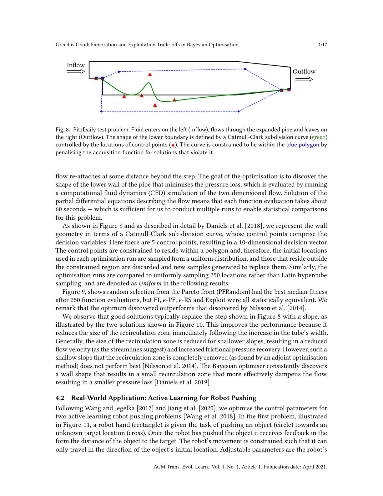
1 Greed is Goo d: Exploration and Exploitation T rade-os in Bayesian Optimisation GEORGE DE A TH, University of Exeter, United Kingdom RICHARD M. EVERSON, University of Exeter, United Kingdom ALMA A. M. RAHA T, Swansea University, United Kingdom JONA THAN E. FIELDSEND, University of Exeter, United Kingdom The performance of acquisition functions for Bayesian optimisation to locate the global optimum of continuous functions is investigated in terms of the Pareto front between exploration and exploitation. W e show that Expected Improvement (EI) and the Upper Condence Bound ( UCB) always select solutions to be expensively evaluated on the Pareto front, but Probability of Improvement is not guaranteed to do so and W eighted Expected Improvement does so only for a restricted range of weights. W e introduce two nov el 𝜖 -greedy acquisition functions. Extensive empirical evaluation of these together with random search, purely exploratory , and purely exploitativ e search on 10 benchmark problems in 1 to 10 dimensions shows that 𝜖 -greedy algorithms are generally at least as eective as conv entional acquisition functions (e .g. EI and UCB), particularly with a limited budget. In higher dimensions 𝜖 -greedy approaches are shown to hav e improved performance over conv entional approaches. These results ar e borne out on a real world computational uid dynamics optimisation problem and a robotics active learning problem. Our analysis and experiments suggest that the most eective strategy , particularly in higher dimensions, is to be mostly greedy , o ccasionally selecting a random exploratory solution. CCS Concepts: • Computing methodologies → Optimization algorithms ; • Theor y of computation → Optimization with randomized search heuristics ; Nonconvex optimization . Additional Ke y W ords and Phrases: Bayesian optimisation, Acquisition function, Inll criteria, 𝜖 -greedy , Exploration-exploitation trade-o. A CM Reference Format: George De Ath, Richard M. Everson, Alma A. M. Rahat, and Jonathan E. Fieldsend. 2021. Greed is Good: Exploration and Exploitation Trade-os in Bayesian Optimisation. A CM Trans. Evol. Learn. 1, 1, Article 1 (April 2021), 22 pages. https://doi.org/10.1145/3425501 1 INTRODUCTION Global function optimisers search for the minimum or maximum of a function by quer ying its value at selecte d locations. All optimisers must therefore balance exploiting knowledge of the function gained from the evaluations thus far with exploring other regions in which the landscape is unknown and might hold b etter solutions. This balance is particularly acute when a limited budget of function evaluations is available , as is often the case in practical problems, e .g. [Jones et al . 1998; Shahriari et al . 2016]. Bayesian optimisation is an eective form of surr ogate-assisted optimisation in which a probabilistic model of the function is constructed from the evaluations made so far . The location at which the function is next (e xpensively) evaluated is chosen as the A uthors’ addresses: George De Ath, g.de.ath@exeter .ac.uk, Department of Computer Science, University of Exeter, Exeter, United Kingdom; Richard M. Everson, r .m.everson@exeter .ac.uk, Department of Computer Science, University of Exeter, Exeter, United Kingdom; Alma A. M. Rahat, a.a.m.rahat@swansea.ac.uk, Department of Computer Science, Swansea University, Swansea, United Kingdom; Jonathan E. Fieldsend, j.e.eldsend@exeter .ac.uk, Department of Computer Science, University of Exeter, Exeter, United Kingdom. © 2021 Copyright held by the owner/author(s). Publication rights licensed to A CM. This is the author’s version of the work. It is posted here for y our personal use . Not for r edistribution. The denitiv e V ersion of Record was published in ACM T ransactions on Evolutionary Learning , https://doi.org/10.1145/3425501. A CM Trans. Evol. Learn., V ol. 1, No. 1, Article 1. Publication date: April 2021. 1:2 George De Ath, Richard M. Everson, Alma A. M. Rahat, and Jonathan E. Fieldsend location which maximises an acquisition function which makes the balance between exploration and exploitation explicit by combining the predicted function value at a location with the uncertainty in that prediction. Here we regard the balance between exploration and exploitation as itself a two-objective optimisation problem. W e show that many , but not all, common acquisition functions eectively select from the Pareto fr ont between objectives quantifying exploration and exploitation. In common with [Bischl et al . 2014; Feng et al . 2015; Grobler et al . 2017; Žilinskas and Calvin 2019], w e propose choosing the next location to b e expensively evaluated from the estimated Pareto set of solutions found by a two-objective evolutionary optimisation of the exploration and exploitation objectives. W e compare the p erformance of various methods for sele cting from the estimated Pareto front and propose two new 𝜖 -greedy schemes that usually cho ose the solutions with the most promising (e xploitative) value, but occasionally use an alternative solution sele cted at random from either the estimated Pareto set or the entire feasible space. Our main contributions can be summarised as follows: • W e present a unied analysis of common acquisition functions in terms of exploration and exploitation and give the rst detailed analysis of weighted expected improvement. • W e investigate the use of the e xploration-exploitation trade-o fr ont in selecting the next location to expensively evaluate in Bayesian optimisation. • W e present two nov el 𝜖 -greedy acquisition functions for Bayesian optimisation as well as other acquisition functions that use the exploration-exploitation trade-o front. • These methods are empirically compared on a variety of synthetic test problems and two real-world applications. • W e demonstrate that the 𝜖 -greedy approaches are at least as eective as the conventional acquisition functions on lower-dimensional problems and be come superior as the number of decision variables increases. W e begin in Section 2 by briey reviewing Bayesian optimisation together with Gaussian processes — which are commonly used for surrogate modelling of the function. W e pay particular attention to acquisition functions and the way in which they balance exploration and exploitation. The exploration-exploitation trade-o is vie wed through the lens of multi-objective optimisation in Section 2.3, which leads to the pr oposed 𝜖 -greedy schemes in Section 3.1. Extensive empirical evaluations on well-known test problems ar e presented in Section 4, along with comparisons on a real world computational uid dynamics optimisation and r obot active learning problem. 2 BA YESIAN OPTIMISA TION Bayesian optimisation (BO) is a particular metho d of surrogate-assisted optimisation. In practice, it has prov ed to be a very eective approach for single objective expensive optimisation problems with limited budget on the number of true function evaluations. It was rst propose d by Kushner [1964] in the early 1960s, and later improv ed and popularised by Močkus et al . [1978] and Jones et al. [1998]. A recent revie w of the topic can be found in [Shahriari et al. 2016]. Without loss of generality , the optimisation problem may be expressed as: max x ∈ X 𝑓 ( x ) , (1) where X ⊂ R 𝑑 is the feasible space and 𝑓 : R 𝑑 → R . Algorithm 1 outlines the standar d Bayesian optimisation procedure. In essence, it is a global search strategy that sequentially samples the design space at likely lo cations of the global optimum taking into account not only the predictions of the surrogate model but also the uncertainty inherent in modelling the unknown function to be optimised [Jones et al . 1998]. It starts (line 1) with a space lling design (e .g. Latin hypercube A CM Trans. Evol. Learn., V ol. 1, No. 1, Article 1. Publication date: April 2021. Greed is Good: Exploration and Exploitation Trade-os in Bayesian Optimisation 1:3 Algorithm 1 Standard Bayesian optimisation. Inputs: 𝑀 : Number of initial samples 𝑇 : Budget on the number of expensive evaluations Steps: 1: 𝑋 ← LatinHypercubeSampling ( X , 𝑀 ) ⊲ Generate initial samples 2: for 𝑡 = 1 → 𝑀 do 3: 𝑓 𝑡 ← 𝑓 ( x 𝑡 ) ⊲ Expensively evaluate all initial samples 4: D ← { ( 𝑋 , f ) } 5: for 𝑡 = 𝑀 + 1 → 𝑇 do 6: 𝜃 ← Train G P ( D ) ⊲ Train a G P model 7: x ′ ← argmax x ∈ X 𝛼 ( x , D , 𝜃 ) ⊲ Maximise inll criterion 8: 𝑓 ′ ← 𝑓 ( x ′ ) ⊲ Expensively evaluate x ′ 9: 𝑋 ← 𝑋 ∪ { x ′ } ⊲ A ugment data 10: f ← f ∪ { 𝑓 ′ } 11: D ← { ( 𝑋 , f ) } 12: return D sampling [McKay et al . 2000]) of the parameter space, constructed independent of the function space. The samples 𝑋 = { x 𝑡 } 𝑀 𝑡 = 1 from this initial design are then (expensively ) evaluated with the function, 𝑓 𝑡 = 𝑓 ( x 𝑡 ) , to construct a training dataset from which the surr ogate model may be learned. W e denote the vector of evaluated samples by f . Then, at each iteration of the main part of the algorithm, a regression model is trained using the function evaluations obtained thus far (line 6). In Bayesian optimisation the regression model is used to predict the most likely value of 𝑓 ( x ) at new lo cations, but also the uncertainty in the model estimate. In common with most work on Bay esian optimisation, we use Gaussian process models (GPs), which subsume Kriging models, as regressors; these are described in Section 2.1. The choice of where to next evaluate 𝑓 is made by nding the location that maximises an acquisition function or inll criterion 𝛼 ( x , D , 𝜃 ) which balances exploitation of goo d regions of design space found thus far with the exploration of promising regions indicated by the uncertainty in the surrogate ’s pr ediction. V arious common inll criteria are discussed and analysed from a multi-objective p oint of view in Section 2.2. The design maximising the inll criterion, x ′ is often found by an evolutionary algorithm ( line 7), which is able to repeatedly evaluate the computationally cheap inll criterion. Finally , 𝑓 ( x ′ ) is expensively evaluated and the training data ( 𝑋 , f ) augmented with x ′ and 𝑓 ( x ′ ) (lines 8 to 10). The process is repeated until the budget is exhausted. 2.1 Modelling with Gaussian Processes Gaussian processes are commonly used to construct a surr ogate model of 𝑓 ( x ) and we therefor e briey describe them here; a compr ehensive introduction may be found in [Rasmussen and Williams 2006]. In essence, a GP is a collection of random variables, and any nite number of these have a joint Gaussian distribution [Rasmussen and Williams 2006]. With data comprising 𝑓 ( x ) evaluated at 𝑀 locations D = { ( x 𝑚 , 𝑓 𝑚 ≜ 𝑓 ( x 𝑚 ) ) } 𝑀 𝑚 = 1 , the predictive probability for 𝑓 at x is a Gaussian distribution with mean 𝜇 ( x ) and variance 𝜎 2 ( x ) : 𝑝 ( 𝑓 | x , D , 𝜃 ) = N ( 𝜇 ( x ) , 𝜎 2 ( x ) ) , (2) A CM Trans. Evol. Learn., V ol. 1, No. 1, Article 1. Publication date: April 2021. 1:4 George De Ath, Richard M. Everson, Alma A. M. Rahat, and Jonathan E. Fieldsend where the mean and variance are 𝜇 ( x ) = 𝜿 ( x , 𝑋 ) 𝐾 − 1 f (3) 𝜎 2 ( x ) = 𝜅 ( x , x ) − 𝜿 ( x , 𝑋 ) ⊤ 𝐾 − 1 𝜅 ( 𝑋 , x ) . (4) Here 𝑋 ∈ R 𝑀 × 𝑑 is the matrix of design locations and f ∈ R 𝑀 is the corresponding vector of the true function evaluations; thus D = { ( 𝑋 , f ) } . The covariance matrix 𝐾 ∈ R 𝑀 × 𝑀 represents the covariance function 𝜅 ( x , x ′ ; 𝜃 ) evaluated for each pair of observations and 𝜿 ( x , 𝑋 ) ∈ R 𝑀 is the vector of co variances b etween x and each of the observations; 𝜃 denotes the kernel hyp erparameters. W e use a e xible class of covariance functions embodie d in the Matérn 5 / 2 kernel, as recommended for modelling realistic functions [Snoek et al . 2012]. Although it is b enecial to marginalise 𝜃 with respect to a prior distribution, here we follow standard practise and x on a single value of the hyperparameters by maximising the log likelihood each time the data is augmente d by a new expensive evaluation: 1 log 𝑝 ( D | 𝜃 ) = − 1 2 log | 𝐾 | − 1 2 f ⊤ 𝐾 − 1 f − 𝑀 2 log ( 2 𝜋 ) . (5) Henceforth, we omit 𝜃 for notational simplicity , and assume that these are set by maximum likelihood estimates. 2.2 Infill Criteria and Multi-Objective Optimisation An inll criterion or acquisition function 𝛼 ( x , D , 𝜃 ) is a measure of quality that enables us to decide which locations x are promising and conse quently where to expensively evaluate 𝑓 . It is based on the prediction 𝑝 ( 𝑓 | x , D ) from the surr ogate (GP) model that represents our belief about the unknown function 𝑓 at a decision vector x based on the 𝑀 observations D . Although 𝛼 ( x , D , 𝜃 ) depends on D and on the hyperparameters ( 𝜃 ) of the GP, for clarity we suppr ess this dependence and write 𝛼 ( x ) . The predictive distribution (2) is Gaussian, with mean and variance given by (3) and (4) . The predicted mean and uncertainty enable an inll criterion to strike a balance b etween myopic exploitation ( concentrating on regions where the mean prediction 𝜇 ( x ) is large) and global exploration (concentrating on regions where the uncertainty 𝜎 ( x ) about 𝑓 is large). Since, in general both exploitation and exploration ar e desirable , w e may view these as competing criteria: a location x that is both more exploitative and more exploratory than an alternative x ′ is to be preferred over x ′ . Using the notation of multi-objective optimisation, a location x dominates x ′ , written x ≻ x ′ , i 𝜇 ( x ) ≥ 𝜇 ( x ′ ) and 𝜎 ( x ) ≥ 𝜎 ( x ′ ) and they are not equal on both. W e present BO procedures that select solutions from the Pareto optimal set of lo cations, namely those which are not dominated by any other feasible locations: P = { x ∈ X | x ′ ⊁ x ∀ x ′ ∈ X } , (6) where x ′ ⊁ x indicates that x ′ does not dominate x . Figure 1 illustrates the approximate Pareto front, { ( 𝜇 ( x ) , 𝜎 ( x ) ) | x ∈ P } , for a simple one- dimensional function. Note that the Pareto set is disjoint in X and in ( 𝜇, 𝜎 ) space. The locations maximising three popular acquisition functions, Expected Improvement (EI), Upper Condence Bound (UCB) and Probability of Improvement (PI) are highlighted. The maximisers of EI and UCB are elements of the Pareto set, wher eas the maximiser of PI is not. W e now present some of the most popular acquisition functions used in BO , and discuss how they achieve a balance between exploration and e xploitation. 1 W e use the L-BFGS algorithm with 10 restarts to estimate the hyper-parameters [GPy 2012]. A CM Trans. Evol. Learn., V ol. 1, No. 1, Article 1. Publication date: April 2021. Gr e e d is Go o d: Exploration and Exploitation T rade-os in Bay esian Optimisation 1:5 0.0 0.2 0.4 0.6 0.8 1.0 x − 0.5 0.0 0.5 1.0 f ( x ) − 0.2 0.0 0.2 0.4 0.6 𝜇 ( x ) 0.0 0.1 0.2 0.3 0.4 𝜎 ( x ) f ( x ) , u n d er l y in g fu n c tion Ev a l u a te d l o c a tion s 𝜇 ( x ) 2 𝜎 ( x ) Pa r eto s et (u p p er ) a n d fr on t ( l o w er ) Domin a te d l o c a tion s Ex p e c te d I mp r o v emen t Up p er Con fid en c e Bou n d Pr ob a b il ity of I mp r o v emen t Fig. 1. Example Par eto fr ont: T op: Gaussian Pr o cess appr o ximation to a function ( blue dashe d cur v e) r esulting fr om the 5 obser vations sho wn; mean 𝜇 ( 𝑥 ) is sho wn in dark gr e en and twice the p osterior standar d de viation 𝜎 ( 𝑥 ) is sho wn as the light gr e en env elop es. Boom: 200 samples uniformly space d in X ploe d in 𝜇 , 𝜎 space . The non-dominate d lo cations forming the Par et o fr ont ar e sho wn in r e d and their lo cations marke d ab o v e . Lo cations maximising the Exp e cte d Impr o v ement, Upp er Confidence Bound and Pr obability of Impr o v ement acquisition functions ar e marke d in b oth plots. 2.2.1 Upp er Confidence Bound. An optimistic p olicy , rst pr op ose d by Lai and Robbins [1985] is to o v er estimate the mean with adde d uncertainty: this is kno wn as the upp er condence b ound inll criterion ( UCB). A pr o of of conv ergence under appr opriate assumptions is giv en in [Srinivas et al . 2010]. The UCB acquisition function is a w eighte d sum of the mean pr e diction and uncertainty: 𝛼 𝑈 𝐶 𝐵 ( x ) = 𝜇 ( x ) +  𝛽 𝑡 𝜎 ( x ) , (7) wher e  𝛽 𝑡 ≥ 0 is the w eight, which generally dep ends up on the numb er of function e valuations, 𝑡 . The addition of a multiple of the uncertainty means that the criterion pr efers lo cations wher e the mean is large ( e xploitation) or mean combine d with the uncertainty is suciently large to warrant e xploration. When 𝛽 𝑡 = 0 UCB b e comes a pur ely e xploitativ e scheme and ther efor e the solution with the b est pr e dicte d mean is e valuate d e xp ensiv ely . Thus, it may rapidly conv erge to a lo cal maximum pr ematur ely . In contrast, when 𝛽 𝑡 is large , the optimisation b e comes pur ely e xplorator y , e valuating A CM T rans. Ev ol. Learn., V ol. 1, No . 1, Article 1. Publication date: April 2021. 1:6 George De Ath, Richard M. Everson, Alma A. M. Rahat, and Jonathan E. Fieldsend − 4 − 2 0 2 4 𝜇 − f ★ 1 2 3 𝜎 UCB − 4 − 2 0 2 4 𝜇 − f ★ EI − 4 − 2 0 2 4 𝜇 − f ★ PI 0.0 0.2 0.4 0.6 0.8 1.0 Fig. 2. Contours of upper confidence b ound (UCB, 𝛽 𝑡 = 1 ), expected improvement (EI) and probability of improvement (PI) as functions of pr edicted mean 𝜇 and uncertainty 𝜎 . Since the scale of 𝛼 is immaterial, all three infill criteria have been mapped to [ 0 , 1 ] . the location where the posterior uncertainty (variance) is largest, which is equivalent to maximally reducing the overall predictive entrop y of the model [Srinivas et al . 2010]. Consequently , it may eventually locate the global optima, but the rate of convergence may be very slow . Some authors suggest tuning 𝛽 𝑡 during the course of the optimisation [Shahriari et al . 2016]; indeed Srinivas et al . ’s convergence proof depends on a particular schedule in which  𝛽 𝑡 increases like the logarithm of 𝑡 , so that more weight is given to exploratory moves as the optimum is approached [Srinivas et al. 2010]. Clearly , UCB increases monotonically as either the mean prediction 𝜇 or the uncertainty 𝜎 increase; see Figure 2. Consequently , if a set S of candidate locations for expensive evaluation is available and 𝛼 𝑈 𝐶 𝐵 is used to select the location with maximum upp er condence bound, x ′ = argmax x ∈ S 𝛼 𝑈 𝐶 𝐵 ( x ) , then x ′ is a member of the maximal non-dominated subset of S ; that is, there is no element of S that dominates x ′ . W e note however , that although UCB selects a non-dominated location, there will generally b e other non-dominate d lo cations that trade-o exploration and exploitation dierently . 2.2.2 Expected Improv ement. The expected improvement (EI) is perhaps the most popular inll criterion and is very widely used. It was rst propose d by Močkus et al . [1978], and further developed by Jones et al . [1998]. Bull has shown that, under certain conditions, BO using EI is guaranteed to converge to the global optimum [Bull 2011]. EI is based on the positive predicted improvement over the best solution 𝑓 ★ = max 𝑚 { 𝑓 𝑚 } observed so far . If ˆ 𝑓 = 𝑓 ( x ) is an evaluation of 𝑓 at x then the improvement is 𝐼 ( x , ˆ 𝑓 , 𝑓 ★ ) = max ( ˆ 𝑓 − 𝑓 ★ , 0 ) . (8) Then the expected improvement at x may b e expressed as [Jones et al. 1998]: 𝛼 𝐸 𝐼 ( x ) = E [ 𝐼 ( x , 𝑓 ★ ) ] = ∫ ∞ −∞ 𝐼 ( x , ˆ 𝑓 , 𝑓 ★ ) 𝑝 ( ˆ 𝑓 | x , D ) 𝑑 ˆ 𝑓 = 𝜎 ( x ) ( 𝑠 Φ ( 𝑠 ) + 𝜙 ( 𝑠 ) ) , (9) where 𝑠 = ( 𝜇 ( x ) − 𝑓 ★ ) / 𝜎 ( x ) is the predicte d improvement at x normalised by the uncertainty , and 𝜙 ( · ) and Φ ( ·) are the standard Gaussian probability density and cumulative density functions. The inll criterion is therefore the impro vement averaged with respect to the posterior predictive probability of obtaining it. Thus, EI balances the exploitation of solutions which are very likely to A CM Trans. Evol. Learn., V ol. 1, No. 1, Article 1. Publication date: April 2021. Greed is Good: Exploration and Exploitation Trade-os in Bayesian Optimisation 1:7 be a little better than 𝑓 ★ with the exploration of others which may , with lower probability , turn out to be much better . As illustrated in Figur e 2, 𝛼 𝐸 𝐼 ( x ) is monotonic with respect to increase in both exploration, 𝜎 , and exploitation, 𝜇 . This can be seen by noting that 𝜕𝛼 𝐸 𝐼 𝜕 𝜇 = Φ ( 𝑠 ) and 𝜕𝛼 𝐸 𝐼 𝜕𝜎 = 𝜙 ( 𝑠 ) (10) are both positive everywhere [Jones et al . 1998]. Consequently , like UCB, if the next location to be expensively evaluated is selected by maximising EI, the location will belong to the Pareto set maximally trading-o exploration and exploitation. 2.2.3 W eighted Expecte d Improv ement. Some authors [Feng et al. 2015; Sóbester et al. 2005] have associated the term, 𝜎 ( x ) 𝑠 Φ ( 𝑠 ) = ( 𝜇 ( x ) − 𝑓 ★ ) Φ ( 𝑠 ) , in (9) with the exploitation inher ent in adopting x as the next place to evaluate . Similarly , the term 𝜎 ( x ) 𝜙 ( 𝑠 ) has be en associate d with the exploratory component. T o control the balance b etween exploration and exploitation Sóbester et al . [2005] dene an acquisition function that weights these two terms dier ently: 𝛼 𝑊 𝐸 𝐼 ( x , 𝜔 ) = 𝜎 ( x ) [ 𝜔 𝑠 Φ ( 𝑠 ) + ( 1 − 𝜔 ) 𝜙 ( 𝑠 ) ] , (11) where 0 ≤ 𝜔 ≤ 1 . Howev er , it turns out that if the next point for expensive e valuation is selected by maximising 𝛼 𝑊 𝐸 𝐼 ( x ) in some set S of candidate solutions, x ′ = argmax x ∈ S 𝛼 𝑊 𝐸 𝐼 ( x , 𝜔 ) , then this only r esults in choosing x ′ in the maximal non-dominated set of S for a relatively small range of 𝜔 . This may be seen by considering the partial derivativ es of 𝛼 𝑊 𝐸 𝐼 ( x , 𝜔 ) . Without loss of generality , we take 𝑓 ★ = 0 , so that 𝑠 = 𝜇 / 𝜎 . Then 𝜕𝛼 𝑊 𝐸 𝐼 𝜕𝜎 = − 𝜔 𝑠 2 𝜙 ( 𝑠 ) + ( 1 − 𝜔 ) ( 𝜙 ( 𝑠 ) − 𝑠 𝜙 ′ ( 𝑠 ) ) (12) =  1 − 𝜔 + ( 1 − 2 𝜔 ) 𝑠 2  𝜙 ( 𝑠 ) , (13) where we have used the fact that 𝜙 ′ ( 𝑠 ) = − 𝑠 𝜙 ( 𝑠 ) . Consequently , when 𝜔 ≤ 1 2 the gradient 𝜕𝛼 𝑊 𝐸 𝐼 𝜕𝜎 > 0 for all 𝑠 . Ho wever , if 𝜔 > 1 2 so that 1 − 2 𝜔 < 0 there are always r egions wher e 𝑠 = 𝜇 / 𝜎 is suciently large that 𝜕𝛼 𝑊 𝐸 𝐼 𝜕𝜎 < 0 . In this case, there are therefore r egions of ( 𝜇, 𝜎 ) space in which decreasing 𝜎 increases 𝛼 𝑊 𝐸 𝐼 , so argmax x ∈ S 𝛼 𝑊 𝐸 𝐼 ( x , 𝜔 ) is not guaranteed to lie in the Pareto set. The gradient in the 𝜇 direction is 𝜕𝛼 𝑊 𝐸 𝐼 𝜕 𝜇 = 𝜔 Φ ( 𝑠 ) + ( 2 𝜔 − 1 ) 𝑠 𝜙 ( 𝑠 ) . (14) Requiring that the gradient is non-negative, so that 𝛼 𝑊 𝐸 𝐼 is non-decreasing with 𝜇 results in: 𝜔 ≥ ( 1 − 2 𝜔 ) 𝑠 𝜙 ( 𝑠 ) Φ ( 𝑠 ) . (15) When 𝜔 > 1 2 it is straightforward to see that (15) is always satised. The inequality is also always satised for all 𝑠 < 0 when 𝜔 < 1 2 . When 𝜔 < 1 2 and 𝑠 ≥ 0 the inequality may b e rewritten as 𝜔 1 − 2 𝜔 ≥ 𝑠 𝜙 ( 𝑠 ) Φ ( 𝑠 ) . (16) Dening 𝛾 = sup 𝑠 𝜙 ( 𝑠 ) Φ ( 𝑠 ) ≈ 0 . 295 , (17) A CM Trans. Evol. Learn., V ol. 1, No. 1, Article 1. Publication date: April 2021. 1:8 George De Ath, Richard M. Everson, Alma A. M. Rahat, and Jonathan E. Fieldsend − 4 − 2 0 2 4 𝜇 − f ★ 1 2 3 𝜎 WEI 𝜔 = 0 − 4 − 2 0 2 4 𝜇 − f ★ WEI 𝜔 = 0.1 − 4 − 2 0 2 4 𝜇 − f ★ WEI 𝜔 = 1 0.0 0.2 0.4 0.6 0.8 1.0 Fig. 3. Contours of weighted expected improvement as functions of the surrogate model’s predicted mean 𝜇 and uncertainty 𝜎 for weights 𝜔 = 0 , 0 . 1 , 1 ; equation (11) . In none of these cases is the x ′ maximising 𝛼 𝑊 𝐸 𝐼 ( x ′ , 𝜔 ) guaranteed to lie in the Pareto set of maximally exploratory and exploitative solutions. it can be seen that 𝜕𝛼 𝑊 𝐸 𝐼 𝜕 𝜇 is only non-negative everywhere if 𝜔 ≥ 𝛾 / ( 2 𝛾 + 1 ) ≈ 0 . 185 . It may therefore be concluded that when 𝜔 ∈ h 𝛾 ( 2 𝛾 + 1 ) , 1 2 i maximising 𝛼 𝑊 𝐸 𝐼 ( x , 𝜔 ) results in the next location for expensive evaluation lying in the Pareto set of available solutions. However , this is not guarante ed for other values of 𝜔 . These results are illustrated in Figure 3, which shows 𝛼 𝑊 𝐸 𝐼 as a function of 𝜇 − 𝑓 ★ and 𝜎 for 𝜔 = 0 , 0 . 1 and 1 ; cf Figure 2 for 𝜔 = 0 . 5 . The complicated nature of 𝛼 𝑊 𝐸 𝐼 is apparent when 𝜔 = 0 . 1 . When 𝜔 = 0 the acquisition function might be expected to yield purely exploratory behaviour . How ever , in this case although lo cations with high variance are preferr ed over those with lo w variance with the same 𝜇 , the acquisition function guides the search to wards locations with high variance but a mean prediction close to 𝑓 ★ . Purely exploitativ e behaviour might be expected when 𝜔 = 1 . In this case the acquisition function is maximised for large 𝜇 and small 𝜎 , which implies that the location with the smaller 𝜎 will b e preferred from two locations with the same 𝜇 . Consequently , although the acquisition function in this case encourages exploitation (preferring large 𝜇 ) it discourages e xploration (preferring small 𝜎 ). This is in contrast to standard EI ( 𝜔 = 0 . 5 , Figure. 2) which prefers the high variance, more exploratory , lo cation from two locations with the same 𝜇 . 2.2.4 Probability of Impr ovement. The Probability of Improvement (PI) is one of the earliest pro- posed inll criteria [Kushner 1964]. It is the pr obability that the prediction at a location x is greater than the best obser ved (expensively evaluated) function value 𝑓 ★ . As the predictive distribution is Gaussian, PI may be calculated in close d form: 𝛼 𝑃 𝐼 ( x ) = 𝑝 ( 𝑓 > 𝑓 ★ | x , D ) = Φ ( 𝑠 ( x ) ) . (18) Thus 𝛼 𝑃 𝐼 ( x ) is the volume of the predictive distribution lying abov e 𝑓 ★ . Since, 𝜕𝛼 𝑃 𝐼 𝜕 𝜇 = 1 𝜎 ( x ) 𝜙 ( 𝑠 ( x ) ) (19) is positive for all 𝜇 ( x ) and 𝜎 ( x ) , PI is monotonically increasing with increasing mean prediction for xed uncertainty . Thus, as might be expe cted, at xed uncertainty , lo cations where the mean is predicted to be large are preferred. Interestingly , as Figure 2 illustrates, such a straightforward monotonic relationship does not exist with respect to uncertainty as shown by 𝜕𝛼 𝑃 𝐼 𝜕𝜎 = − 𝑠 ( x ) 𝜙 ( 𝑠 ( x ) ) . (20) A CM Trans. Evol. Learn., V ol. 1, No. 1, Article 1. Publication date: April 2021. Greed is Good: Exploration and Exploitation Trade-os in Bayesian Optimisation 1:9 When the improv ement in the mean is negative 𝑠 ( x ) < 0 then (20) shows that PI increases with uncertainty 𝜎 . Howev er , in contrast to EI and UCB, when 𝜇 ( x ) > 𝑓 ★ then (20) shows that PI decreases with 𝜎 ; tha locations with small uncertainty are preferred to those with high uncertainty . Therefore , the location x ′ selected by PI is not guarante ed to be a member of the maximal non- dominated set of candidates. In other words, there may be candidate locations x ′′ which are more exploratory ( 𝜎 ( x ′′ ) > 𝜎 ( x ′ ) ) while having the same mean prediction ( 𝜇 ( x ′′ ) = 𝜇 ( x ′ ) ) as the x ′ selected by PI. In practice, such behaviour leads to an overly exploitative scheme, see for example [Jones 2001]. T o combat this exploitative nature , usually a higher target than the best obser ved value, 𝑓 ★ , is set for computing the pr obability of improvement. This often improves the performance of PI-based BO [Jones 2001; Kushner 1964; Lizotte 2008]. As Figure 2 shows, this can be attributed to the fact that solutions are evaluated as if their impr ovement wer e negative where the PI criterion encourages exploration as well as exploitation. Although this modication tends to improv e performance, there is, howev er , no natural choice for a suitable high target. 2.3 Exploration and Exploitation Trade-o As discussed above, the EI and UCB inll criteria select the next location to be expensively evaluated as one of the locations that are members of the maximal non-dominated set of available locations, namely P (6) , the Pareto set resulting from simultaneous maximisation of 𝜇 ( x ) and 𝜎 ( x ) . PI only selects from P when 𝜇 ( x ) < 𝑓 ★ and in practice an articially high 𝑓 ★ is used to promote exploration. Note, howev er , that EI and UCB select from dierent regions of the Pareto set, balancing exploitation and exploration dierently . Indeed, the proof of convergence for BO with UCB relies on varying the selection position along the Pareto fr ont as the optimisation procee ds, becoming more exploratory in later stages [Srinivas et al. 2010]. Inspection of Figure 2 shows that EI is more exploitative than UCB in the sense that if the solutions available for selection all have the same upper condence bound, that is they lie on a contour of 𝛼 𝑈 𝐶 𝐵 , then maximising 𝛼 𝐸 𝐼 will choose the most exploitative of them. Conversely , if the available solutions all have the same EI, then maximising 𝛼 𝑈 𝐶 𝐵 will choose the most exploratory . 3 U TILISING THE EXPLORA TION VS. EXPLOIT A TION TRADE-OFF FRONT Previous w orks [Bischl et al . 2014; Feng et al . 2015; Grobler et al . 2017] have used the exploration vs. exploitation (EE) fr ont in a batch setting, in which multiple locations in the EE Pareto set are selected to be evaluated in parallel. Feng et al . [2015] use the two weighted components of 𝛼 𝑊 𝐸 𝐼 (11) as the two objectives dening a trade-o front that is appr oximated via the use of a multi-objective evolutionary algorithm (MOEA). They select batches of 𝑞 solutions to be expensively evaluated in parallel by choosing the two extremal solutions of the approximated Pareto set and the remaining 𝑞 − 2 locations equally spread (in objective space) across the set. Grobler et al . [2017] replace the 𝛼 𝑊 𝐸 𝐼 formulation with a trade-o front consisting of the surrogate model’s mean and variance, again using a MOEA to approximate the Par eto set. They select a batch of locations consisting of the two extremal solutions of the set, together with the lo cation that maximises EI, and equally spaced solutions across the set. Bischl et al . [2014] consider the maximisation of an additional objective, namely the decision space distance to each solution’s nearest neighbour , thus promoting exploration. They also limit the size of the MOEA p opulation to be the batch size in order to avoid the problem of explicitly selecting a batch of locations from a large Pareto set. The use of the EE front in the sequential setting is much less explored. Howev er , Žilinskas and Calvin [2019] have recently highlighted the importance of visualising of the EE front to b etter inform model selection and they recommend that future researchers should aim to e xploit the EE front further . A CM Trans. Evol. Learn., V ol. 1, No. 1, Article 1. Publication date: April 2021. 1:10 George De Ath, Richard M. Everson, Alma A. M. Rahat, and Jonathan E. Fieldsend Algorithm 2 𝜖 -greedy acquisition functions. (2a) 𝜖 -PF: Pareto front selection. 1: if rand ( ) < 𝜖 then 2: ˜ P ← MOOptimise x ∈ X ( 𝜇 ( x ) , 𝜎 ( x ) ) 3: x ′ ← randomChoice ( ˜ P ) 4: else 5: x ′ ← argmax x ∈ X 𝜇 ( x ) (2b) 𝜖 -RS: Random selection from feasible space. 1: if rand ( ) < 𝜖 then 2: x ′ ← randomChoice ( X ) 3: else 4: x ′ ← argmax x ∈ X 𝜇 ( x ) Here we focus on the sequential BO framew ork (r ecall Algorithm 1) and consider algorithms that select the next location for expensive evaluation from the entire Pareto set of feasible locations. Use of an ecient evolutionary multi-obje ctive search algorithm means that nding an approximation ˜ P to P has ab out the same computational expense as maximising a scalar acquisition function such as EI or UCB directly . In this work the approximate Pareto set of model predictions is found using a standard ev olutionary optimiser , NSGA -II [Deb et al. 2001]. W e note that while proofs of convergence for particular trade-os between exploration and exploitation exist [Bull 2011; Srinivas et al . 2010], it is clear that merely selecting locations for any xed exploration-exploitation weighting are not guaranteed to converge. At the two extremes, purely exploitative schemes sele ct x ′ = argmax x ∈ X 𝜇 ( x ) and purely exploratory schemes select x ′ = argmax x ∈ X 𝜎 ( x ) . The former are liable to b ecome stuck at lo cal optima, while the latter visits each location with the maximum posterior variance 𝜎 2 ( x ) , thus reducing the uncertainty of the model, as quantied by the entropy of the predictive posterior . This will lead to the ev entual location of the optimum, but only very slowly as ev en very unpromising locations wher e 𝜇 ( x ) ≪ 𝑓 ★ are visited. In Section 4 we evaluate the performance of the purely exploitativ e and exploratory strategies, denoted Exploit and Explore respectively . Since all solutions in the Pareto set may be considered equally good and dominate all other feasible lo cations, we also consider the PFRandom algorithm, which selects a solution at random from ˜ P for the next expensive evaluation. As discussed above , the maximally e xploratory strategy will converge to the global optimum, but very slowly . At the other extreme of the Pareto front, a greedy , exploitative, strategy , while converging quickly , risks becoming stuck at a lo cal optimum. In the next section, therefore, we seek to capitalise on the rapid conv ergence of the exploitative strategy while avoiding local minima by making occasional exploratory moves. 3.1 𝜖 -Greedy Bayesian Optimisation Motivated by the success of 𝜖 -greedy schemes in reinforcement learning [Mnih et al . 2015; Sutton and Barto 1998; T okic 2010; van Hasselt et al . 2016], w e propose two novel BO acquisition functions which use the 𝜖 -greedy methodology to sele ct the next p oint for expensive evaluation. Both metho ds mostly select the most exploitative solution, but dier in which exploratory solution is sele cted in a small proportion of steps. The rst method which we denote 𝜖 -PF and is summarised in Algorithm 2a, usually selects the location x ′ with the most promising mean prediction from the surrogate model. In the remaining cases, with probability 𝜖 , it selects a random lo cation from the approximate Pareto set ˜ P , thus usually selecting a more exploratory x ′ instead of the most exploitative location available. The function MOOptimise denotes the use of a multi-objective optimiser to generate ˜ P . This acquisition function replaces line 7 in standard BO , Algorithm 1. A CM Trans. Evol. Learn., V ol. 1, No. 1, Article 1. Publication date: April 2021. Greed is Good: Exploration and Exploitation Trade-os in Bayesian Optimisation 1:11 Name Domain 𝑑 W angFreitas [W ang and de Freitas 2014] [ 0 , 1 ] 1 Branin † [ − 5 , 0 ] × [ 10 , 15 ] 2 BraninForrester [Forrester et al. 2008] [ − 5 , 0 ] × [ 10 , 15 ] 2 Cosines [González et al. 2016b] [ 0 , 0 ] × [ 5 , 5 ] 2 logGoldsteinPrice † [ − 2 , − 2 ] × [ 2 , 2 ] 2 logSixHumpCamel † [ − 3 , 2 ] × [ 3 , 2 ] 2 logHartmann6 † [ 0 , 1 ] 𝑑 6 logGSobol [González et al. 2016a] [ − 5 , 5 ] 𝑑 10 logRosenbrock † [ − 5 , 10 ] 𝑑 10 logStyblinskiT ang † [ − 5 , 5 ] 𝑑 10 T able 1. Functions used in these experiments, along with their domain and dimensionality , 𝑑 . Formulae can be found as cited or at http://www .sfu.ca/~ssurjano/optimization.html for those labelled with † . Full details of all evaluated functions can also be found in the supplementary material. The 𝜖 -RS scheme, summarised in Algorithm 2b, also usually sele cts x ′ with the most promising mean prediction from the surr ogate. How ever , with probability 𝜖 a location is randomly selected (hence the abbreviation 𝜖 -RS) from the entire feasible space X . Selection of x ′ from ˜ P ( 𝜖 -PF, Algorithm 2a) might be expected to be more ee ctive than selecting x ′ from the entire feasible space ( 𝜖 -RS, Algorithm 2b) because a selection from X is likely to be dominated by ˜ P and therefor e is likely to be less exploratory and less exploitative. W e remark that these 𝜖 -greedy schemes are dierent to that proposed by Bull [2011], which greedily selects the lo cation with maximum expected improvement with probability 1 − 𝜖 , and randomly chooses a location the remainder of the time. This is dierent fr om our proposals because the Bull scheme greedily maximises EI rather than exploitation ( 𝜇 ). 4 EXPERIMENT AL EV ALU A TION W e investigate the performance of the two propose d 𝜖 -greedy methods, 𝜖 -PF and 𝜖 -RS, by evaluating them on ten b enchmark functions with a range of domain sizes and dimensionality; see T able 1 for details. Note that the benchmarks are couched as minimisation problems. In common with other works [Jones et al . 1998; Schonlau 1997; W agner and W essing 2012; W ang et al . 2015], the functions prexed with log are log-transformed, i.e. the logarithm of each observed values log ( 𝑓 ( x ) ) is modelled rather than observed value 𝑓 ( x ) itself. Where the observations can b e negative , a constant larger than minimum value of the function is added. 2 These functions are transformed in this gre y- box fashion, using a small amount of prior information about the scales of the function, because we want the surrogate model to be as accurate as possible. As discussed in the seminal work of Jones et al . [1998], it is often possible to improve poorer surrogate model ts, as one typically observes with the untransformed functions, by using the log transformation. The equations dening each transformed function and optimisation results of all methods on the untransformed functions are available in the supplementary material. W e discuss the dierences in optimisation performance between the standard and log-transformed functions below . W e compare the two proposed metho ds to the purely exploitative and exploratory strategies, denoted Exploit and Explore respe ctively , as well as random selection from the approximated 2 W e have used prior information on the function’s minimum value to choose the constant, but the actual value is immaterial because the function obser vations are in any case standardised as part of the GP modelling. A CM Trans. Evol. Learn., V ol. 1, No. 1, Article 1. Publication date: April 2021. 1:12 George De Ath, Richard M. Everson, Alma A. M. Rahat, and Jonathan E. Fieldsend Method W angFreitas (1) BraninForrester (2) Branin (2) Cosines (2) logGoldsteinPrice (2) Median MAD Me dian MAD Me dian MAD Median MAD Median MAD LHS 1 . 27 × 10 − 2 1 . 80 × 10 − 2 4 . 59 × 10 − 1 4 . 73 × 10 − 1 1 . 31 × 10 − 1 1 . 33 × 10 − 1 4 . 79 × 10 − 1 2 . 71 × 10 − 1 1 . 08 7 . 69 × 10 − 1 Explore 1 . 04 × 10 − 2 1 . 42 × 10 − 2 4 . 58 × 10 − 1 3 . 52 × 10 − 1 1 . 66 × 10 − 1 1 . 56 × 10 − 1 4 . 56 × 10 − 1 2 . 20 × 10 − 1 1 . 01 5 . 50 × 10 − 1 EI 2 . 00 6 . 91 × 10 − 11 2 . 47 × 10 − 6 3 . 23 × 10 − 6 4 . 15 × 10 − 6 3 . 76 × 10 − 6 6 . 31 × 10 − 6 7 . 68 × 10 − 6 2 . 73 × 10 − 6 3 . 34 × 10 − 6 PI 2 . 06 8 . 24 × 10 − 2 3 . 73 × 10 − 4 3 . 70 × 10 − 4 2 . 26 × 10 − 5 3 . 22 × 10 − 5 2 . 50 × 10 − 3 3 . 18 × 10 − 3 2 . 92 × 10 − 3 4 . 32 × 10 − 3 UCB 2 . 00 1 . 26 × 10 − 11 4 . 96 × 10 − 6 6 . 22 × 10 − 6 4 . 42 × 10 − 6 4 . 06 × 10 − 6 7 . 12 × 10 − 6 8 . 86 × 10 − 6 6 . 15 × 10 − 6 6 . 17 × 10 − 6 PFRandom 2 . 00 × 10 − 4 2 . 96 × 10 − 4 2 . 70 × 10 − 3 3 . 65 × 10 − 3 1 . 67 × 10 − 3 2 . 17 × 10 − 3 8 . 82 × 10 − 3 1 . 14 × 10 − 2 2 . 54 × 10 − 3 3 . 31 × 10 − 3 𝜖 -RS 1 . 04 × 10 − 6 1 . 54 × 10 − 6 2 . 00 × 10 − 6 2 . 49 × 10 − 6 3 . 17 × 10 − 6 2 . 46 × 10 − 6 8 . 66 × 10 − 6 1 . 21 × 10 − 5 2 . 33 × 10 − 6 2 . 36 × 10 − 6 𝜖 -PF 2 . 00 3 . 72 × 10 − 11 2 . 31 × 10 − 6 3 . 01 × 10 − 6 3 . 57 × 10 − 6 3 . 13 × 10 − 6 2 . 02 × 10 − 6 2 . 52 × 10 − 6 8 . 76 × 10 − 7 1 . 08 × 10 − 6 Exploit 2 . 00 6 . 00 × 10 − 9 4 . 61 × 10 − 6 6 . 04 × 10 − 6 3 . 08 × 10 − 6 3 . 29 × 10 − 6 4 . 13 × 10 − 1 6 . 12 × 10 − 1 2 . 26 × 10 − 6 2 . 90 × 10 − 6 Method logSixHumpCamel (2) logHartmann6 (6) logGSobol (10) logRosenbrock (10) logStyblinskiT ang (10) Median MAD Me dian MAD Me dian MAD Median MAD Median MAD LHS 6 . 52 1 . 10 3 . 37 × 10 − 1 1 . 10 × 10 − 1 1 . 51 × 10 1 9 . 03 × 10 − 1 1 . 16 × 10 1 5 . 39 × 10 − 1 2 . 85 1 . 77 × 10 − 1 Explore 6 . 53 1 . 24 3 . 07 × 10 − 1 6 . 85 × 10 − 2 1 . 75 × 10 1 1 . 42 1 . 28 × 10 1 4 . 82 × 10 − 1 3 . 19 1 . 13 × 10 − 1 EI 7 . 42 × 10 − 5 9 . 19 × 10 − 5 1 . 06 × 10 − 3 6 . 73 × 10 − 4 7 . 15 1 . 58 6 . 62 6 . 58 × 10 − 1 2 . 34 2 . 79 × 10 − 1 PI 1 . 46 × 10 − 1 1 . 58 × 10 − 1 6 . 15 × 10 − 4 7 . 69 × 10 − 4 6 . 29 1 . 61 6 . 89 9 . 49 × 10 − 1 2 . 29 2 . 37 × 10 − 1 UCB 3 . 84 1 . 36 2 . 04 × 10 − 1 3 . 21 × 10 − 2 1 . 45 × 10 1 6 . 16 × 10 − 1 8 . 31 5 . 90 × 10 − 1 3 . 19 1 . 13 × 10 − 1 PFRandom 1 . 52 × 10 − 1 1 . 52 × 10 − 1 6 . 57 × 10 − 2 3 . 27 × 10 − 2 5 . 60 1 . 73 5 . 23 4 . 98 × 10 − 1 2 . 70 3 . 15 × 10 − 1 𝜖 -RS 3 . 81 × 10 − 5 2 . 96 × 10 − 5 5 . 09 × 10 − 4 3 . 59 × 10 − 4 5 . 13 1 . 86 4 . 75 7 . 85 × 10 − 1 1 . 61 3 . 12 × 10 − 1 𝜖 -PF 4 . 06 × 10 − 5 4 . 66 × 10 − 5 7 . 71 × 10 − 4 4 . 82 × 10 − 4 5 . 06 1 . 37 4 . 64 6 . 25 × 10 − 1 1 . 53 4 . 49 × 10 − 1 Exploit 4 . 21 × 10 − 5 4 . 95 × 10 − 5 6 . 37 × 10 − 4 5 . 82 × 10 − 4 5 . 27 1 . 60 4 . 54 6 . 19 × 10 − 1 1 . 82 3 . 71 × 10 − 1 T able 2. Me dian absolute distance ( le ) and median absolute deviation from the median (MAD, right ) from the optimum aer 250 function evaluations across the 51 runs. The method with the lowest median performance is shown in dark grey , with those with statistically e quivalent performance are shown in light gre y . Pareto front, PFRandom . Their p erformance is also compared to the inll criteria discussed in Section 2.2, namely Expecte d Improv ement (EI), Upper Condence Bound (UCB) and Probability of Impro vement (PI). In addition, we compare the performance of all the inll criteria with the quasi-random search produced by max-min Latin Hyp ercube Sampling (LHS, [McKay et al . 2000]). LHS is the generalisation of a Latin square, in which samples are placed in rows and columns of a square such that each sample r esides in its own row and column. The max-min variant of LHS tries to maximise the minimum distance between each sample. The methods were evaluated on the synthetic b enchmark functions in T able 1, with a budget of 250 function evaluations that included 𝑀 = 2 𝑑 initial LHS samples (Algorithm 1, Line 1). T o allow statistical performance measures to be used, each optimisation was repeated 51 times. The same sets of initial samples were used for each method’s runs to allow for paired statistical comparisons between the metho ds to be carried out. In all experiments a value of 𝜖 = 0 . 1 was used for both 𝜖 -PF and 𝜖 -RS. The UCB algorithm was run with 𝛽 𝑡 adjusted according to the schedule dened for continuous functions in Theorem 2 of Srinivas et al . [2010] with 𝑎 = 𝑏 = 1 and 𝛿 = 0 . 01 . All acquisition functions were optimised with NSGA-II [Deb et al . 2001], apart from PI which was optimised following the common practise [Balandat et al . 2020; GPyOpt 2016] of uniformly sampling X and optimising the 10 most promising locations with L-BFGS-B [Byr d et al . 1995]. In both cases the optimisation budget was 5000 𝑑 evaluations. The multi-start strategy was used to optimise PI be cause, as shown in Section 2.2.4, the maximiser of PI may not lie in the Pareto set of 𝜇 ( x ) and 𝜎 ( x ) . For NSGA -II, we set the parameters to commonly used values: the population size was 100 𝑑 , the numb er of generations was 50 (100 generations lead to no signicant improvement in performance), the crossov er and mutation probabilities were 0 . 8 and 1 𝑑 respectively , and both the distribution indices for crossov er and mutation were 20 . T able 2 shows the median regr et, i.e. the median dierence between the estimated optimum 𝑓 ★ and the true optimum over the 51 repeated experiments, together with the median absolute deviation A CM Trans. Evol. Learn., V ol. 1, No. 1, Article 1. Publication date: April 2021. Greed is Good: Exploration and Exploitation Trade-os in Bayesian Optimisation 1:13 LH S Ex p l or e EI PI UCB PF Ra n d om 𝜖 -RS 𝜖 -PF Ex p l oit 10 − 8 10 − 6 10 − 4 10 − 2 10 0 Reg r et W a n g F r eita s (1) 10 − 5 10 − 3 10 − 1 10 1 Br a n in (2) 0 50 100 150 200 250 F u n c tion Ev a l u a tion s 1.5 2.0 2.5 3.0 Reg r et l og S ty b l in s kiT a n g (10) 0 50 100 150 200 250 F u n c tion Ev a l u a tion s 4.0 6.0 8.0 10.0 12.0 l og Ros en b r o c k (10) Fig. 4. Illustrative convergence plots for four benchmark problems. Each plot sho ws the median dierence be- tween the best function value seen and the true optimum (regret), with shading r epresenting the interquartile range across the 51 runs. The dashed vertical line indicates the end of the initial LHS phase. from the me dian (MAD). The method with the lowest ( best) median regret on each function is highlighted in dark grey , and those which are statistically e quivalent to the best metho d according to a one-sided paired Wilcoxon signed-rank test [Knowles et al . 2006] with Holm-Bonferroni correction [Holm 1979] ( 𝑝 ≥ 0 . 05 ), are shown in light grey . Figure 4 shows the convergence of the various algorithms on four illustrative test pr oblems in 𝑑 = 1 , 2 and 10 dimensions. Convergence plots for all the benchmark problems are available in the supplementary material, and Python code to generate gures and repr oduce all experiments is available online 3 . As might be e xpecte d, Latin Hypercube Sampling (LHS) and purely exploratory search (Explor e), which have roughly equivalent performance, are not the best metho ds on any of the test problems. Perhaps surprisingly , none of the three well-known acquisition functions, EI, UCB and PI, has the best median performance after 250 evaluations, although all three are statistically equivalent to the best method on 𝑑 = 2 Cosines, and EI and UCB have goo d performance on the 𝑑 = 2 Branin and BraninForrester problems. In contrast, the 𝜖 -greedy algorithms 𝜖 -PF and 𝜖 -RS perform well across the range of problems, particularly on the higher-dimensional pr oblems. Interestingly , Exploit, which always samples from the b est mean surrogate prediction is competitive for most of the high dimensional problems. This indicates one of the main conclusions of this work, namely that as the dimension of decision space increases the approximate mo delling of 𝑓 ( x ) is so poor that even adopting the modelled most-exploitative solution inherently leads to some (unintended) exploration. While pure exploitation combined with fortuitous exploration appears to be a good strategy for many problems, introducing some deliberate exploration can b e imp ortant. This is particularly 3 https://github.com/georgedeath/egreedy/ A CM Trans. Evol. Learn., V ol. 1, No. 1, Article 1. Publication date: April 2021. 1:14 George De Ath, Richard M. Everson, Alma A. M. Rahat, and Jonathan E. Fieldsend 10 − 7 10 − 4 10 − 1 Reg r et Cos in es ( 2 ) : T = 50 Cos in es ( 2 ) : T = 150 Cos in es ( 2 ) : T = 250 10 − 5 10 − 3 10 − 1 10 1 Reg r et l og S ix H u mp Ca mel ( 2 ) : T = 50 l og S ix H u mp Ca mel ( 2 ) : T = 150 l og S ix H u mp Ca mel ( 2 ) : T = 250 LH S Ex p l or e EI PI UCB PF Ra n d om 𝜖 -RS 𝜖 -PF Ex p l oit 5.0 10.0 15.0 20.0 Reg r et l og GS ob ol ( 10 ) : T = 50 LH S Ex p l or e EI PI UCB PF Ra n d om 𝜖 -RS 𝜖 -PF Ex p l oit l og GS ob ol ( 10 ) : T = 150 LH S Ex p l or e EI PI UCB PF Ra n d om 𝜖 -RS 𝜖 -PF Ex p l oit l og GS ob ol ( 10 ) : T = 250 Fig. 5. Distribution of the best-seen function values aer 50 ( le ), 150 ( centre ) and 250 ( right ) function evaluations on three benchmark problems. apparent on the W angFreitas problem [W ang and de Freitas 2014] which contains a large local optimum and a narrow global optimum that is surrounded by plateaux; see supplementary material for a plot. Convergence on this problem is shown in Figure 4, which demonstrates how LHS sampling and a purely exploratory strategy (Explore) converge slowly towards the optimum, while Exploit fails to nd the vicinity of the optimum in any case. On the other hand, the deliberate exploratory moves incorporated in b oth 𝜖 -greedy methods and PFRandom (random selection from the Pareto set) enable some of the runs to converge to the optimum. The 𝜖 -RS method, which makes exploratory moves from the entire feasible space , is most eective, although as discussed below , generally we nd 𝜖 -PF to be more eective. Figure 5 shows the distribution of the best-seen function evaluations for each of the evaluated algorithms on three benchmark problems for budgets of 𝑇 = 50 , 150 and 250 function evaluations. Again, w e see in the two-dimensional Cosines and logSixHumpCamel plots that driving the optimi- sation process solely by e xploiting the surrogate ’s mean pr ediction can fail to correctly identify the optimum because the model is inaccurate and may miss, for example , a small scale optimum. When 𝑓 is modelled poorly , then the mean function will not accurately represent the true function. Howev er , as is the case with the logGSobol plot and indeed the other ten-dimensional functions, pure exploitation can provide a sucient driver for optimisation, b ecause the inaccurate and changing surrogate (as new evaluations become available) induces sucient exploration. W e note howev er , that the 𝜖 -greedy algorithms, incorp orating deliberate exploration, oer more consistent performance. A CM Trans. Evol. Learn., V ol. 1, No. 1, Article 1. Publication date: April 2021. Greed is Good: Exploration and Exploitation Trade-os in Bayesian Optimisation 1:15 10 − 7 10 − 4 10 − 1 Reg r et Cos in es (2): T = 50 Cos in es (2): T = 150 Cos in es (2): T = 250 5.0 10.0 15.0 Reg r et l og GS ob ol (10): T = 50 l og GS ob ol (10): T = 150 l og GS ob ol (10): T = 250 0.01 0.05 0.1 0.2 0.3 0.4 0.5 4.0 6.0 8.0 10.0 12.0 Reg r et l og Ros en b r o c k (10): T = 50 0.01 0.05 0.1 0.2 0.3 0.4 0.5 l og Ros en b r o c k (10): T = 150 0.01 0.05 0.1 0.2 0.3 0.4 0.5 l og Ros en b r o c k (10): T = 250 Fig. 6. Comparison of 𝜖 -PF ( green ) and 𝜖 -RS ( red, hatched ) for dierent values of 𝜖 (horizontal axis) aer 50 ( le ), 150 ( centre ) and 250 ( right ) function evaluations. A common trend apparent across the both Figures 4 and 5 is that EI tends to initially improv e at a slower rate than the two 𝜖 -greedy methods, but then catches up to a greater or lesser extent after more function evaluations. This is well illustrated in the logSixHumpCamel plot in Figure 5 and also in the Branin and logRosenbrock plots in Figure 4. UCB performs poorly on the higher dimensional functions. This may be due to the value of 𝛽 𝑡 used, as the convergence proofs in [Srinivas et al . 2010] rely on 𝛽 𝑡 increasing with the dimensionality of the problem, leading to o ver-exploration. One may argue that this can be ov ercome by simply using a smaller 𝛽 𝑡 value, set in some ad hoc manner . However , with no a priori knowledge as to how to select the parameter on a per-problem basis, we suggest that this is not a feasible strategy in practice. How greedy? Choosing 𝜖 . Although the 𝜖 -greedy algorithms perform well in comparison with conventional acquisition functions, it is unclear what value of 𝜖 to choose, and indee d whether the exploratory moves should choose from the approximate Pareto fr ont ( 𝜖 -PF) or fr om the entire feasi- ble space ( 𝜖 -RS) which is marginally cheaper . Figure 6 illustrates the eect of 𝜖 on the performance of 𝜖 -PF (gr een) and 𝜖 -RS (red, hatched). As is clear from the Cosines problem, a larger value of 𝜖 may be required to avoid getting stuck because the surrogate is not modelling the function well enough and needs a larger number of exploratory samples. However , there is very little change in performance with 𝜖 for the higher dimensional decision spaces (e .g. logGSobol and logRosenbrock). As suggested above w e attribute this to the inaccurate surrogate modelling in higher dimensions which leads to a large degree of random search irrespective of 𝜖 . Interestingly , this is not the case for these functions without the log transformation (Rosenbrock and GSobol). Figure 7 shows the performance of 𝜖 -RS and 𝜖 -PF for dierent values of 𝜖 on the A CM Trans. Evol. Learn., V ol. 1, No. 1, Article 1. Publication date: April 2021. 1:16 George De Ath, Richard M. Everson, Alma A. M. Rahat, and Jonathan E. Fieldsend 0.01 0.05 0.1 0.2 0.3 0.4 0.5 10 1 10 3 10 5 Reg r et GS ob ol (10): T = 50 0.01 0.05 0.1 0.2 0.3 0.4 0.5 GS ob ol (10): T = 150 0.01 0.05 0.1 0.2 0.3 0.4 0.5 GS ob ol (10): T = 250 Fig. 7. A comparison of optimising the GSobol function with 𝜖 -PF ( green ) and 𝜖 -RS ( red, hatched ) for dier ent values of 𝜖 ( horizontal axis) aer 50 ( le ), 150 ( centre ) and 250 ( right ) function evaluations. GSobol problem. As can be seen in the gure , increasing 𝜖 decreases the performance of 𝜖 -PF and increases the performance of 𝜖 -RS, in stark contrast to logGSobol in Figur e 6. This indicates that the surrogate model is misleading the optimisation because increasing the frequency of expensively evaluating random locations and decreasing the frequency of sampling from the Pareto front both improv e optimisation. In this case, the log transformation enables more accurate mo delling of the objective and thus more rapid optimisation. Overall, setting 𝜖 = 0 . 1 app ears to be large enough to give good performance across all pr oblems (see supplementar y material for results on other problems), particularly for the 𝜖 -PF algorithm. Larger values give no real improvement in performance. Empirically it appears that 𝜖 -PF gives marginally better performance than 𝜖 -RS, as might be expected if the surrogate describes 𝑓 well, as is the case in the later stages of optimisation. In this case, selection from the appr oximate Pareto front yields solutions that lie on the maximal trade-o between exploration and exploitation and may therefore be expected to yield the most information. Ho wever , in cases where the surrogate modelling is particularly poor throughout the entire optimisation run, as is the case in sev eral of the test problems without log transformation, the incr eased stochasticity provided by 𝜖 -RS with larger values of 𝜖 appears useful in overcoming the misleading surr ogate model. Results on the black-box test problems. Here we briey describ e the optimisation results of the evaluated methods on the six test problems without log transformation – full results are available in the supplementary material. The 𝜖 -RS method is the best performing or statistically e quivalent to the best p erforming method on all six of the b enchmark problems, with 𝜖 -PF best or e quivalent on ve of the six. EI, PI and Exploit were all the b est or equivalent to the b est performing on three of the six test problem. As noted above, 𝜖 -RS performs better than 𝜖 -PF on the higher dimensional problems, with the two methods giving equivalent performance on the low er dimensional problems. The main dierence of the standar d acquisition functions is that performance is closer to that of the 𝜖 -greedy methods than on the log-transformed functions. W e attribute this to be a result of poorer surrogate modelling in the presence of a wide range of objective values so that the 𝜖 -greedy schemes are less able to exploit the model’s mean predicted value 𝜇 ( x ) . W e reiterate here, how ever , that the performance of b oth 𝜖 -RS and 𝜖 -PF across the untransformed b enchmark functions is still superior to the standard acquisition functions. 4.1 Real- W orld Application: Pipe Shap e Optimisation W e also evaluate the range of acquisition functions on a real-world computational uid dynamics optimisation problem. As illustrated in Figur e 8, the PitzDaily test problem [Daniels et al . 2018] involves optimising the shap e of a pipe in order to reduce the pressure loss between the inow and outow . Pressure loss is caused by a rapid expansion in the pipe (a backward-facing step), which forces the ow to separate at the edge of the step, creating a r ecirculation zone, before the A CM Trans. Evol. Learn., V ol. 1, No. 1, Article 1. Publication date: April 2021. Gr e e d is Go o d: Exploration and Exploitation T rade-os in Bay esian Optimisation 1:17 Ino w Outo w Fig. 8. PitzDaily test pr oblem. F luid enters on the le (Inf lo w ), f lo ws thr ough the e xpande d pip e and leav es on the right ( Outf lo w ) . The shap e of the lo w er b oundar y is define d by a Catmull-Clark sub division cur v e ( gr e en ) contr olle d by the lo cations of contr ol p oints ( ▲ ). The cur v e is constraine d to lie within the blue p olygon by p enalising the acquisition function for solutions that violate it. o w r e-attaches at some distance b e y ond the step . The goal of the optimisation is to disco v er the shap e of the lo w er w all of the pip e that minimises the pr essur e loss, which is e valuate d by running a computational uid dynamics ( CFD ) simulation of the tw o-dimensional o w . Solution of the partial dier ential e quations describing the o w means that each function e valuation takes ab out 60 se conds — which is sucient for us to conduct multiple runs to enable statistical comparisons for this pr oblem. A s sho wn in Figur e 8 and as describ e d in detail by Daniels et al . [2018], w e r epr esent the wall ge ometr y in terms of a Catmull-Clark sub-division cur v e , whose contr ol p oints comprise the de cision variables. Her e ther e ar e 5 contr ol p oints, r esulting in a 10-dimensional de cision v e ctor . The contr ol p oints ar e constraine d to r eside within a p olygon and, ther efor e , the initial lo cations use d in each optimisation run ar e sample d fr om a uniform distribution, and those that r eside outside the constraine d r egion ar e discar de d and ne w samples generate d to r eplace them. Similarly , the optimisation runs ar e compar e d to uniformly sampling 250 lo cations rather than Latin hyp er cub e sampling, and ar e denote d as Uniform in the follo wing r esults. Figur e 9, sho ws random sele ction fr om the Par eto fr ont (PFRandom) had the b est me dian tness after 250 function e valuations, but EI, 𝜖 -PF, 𝜖 -RS and Exploit w er e all statistically e quivalent. W e r emark that the optimum disco v er e d outp erforms that disco v er e d by Nilsson et al. [2014]. W e obser v e that go o d solutions typically r eplace the step sho wn in Figur e 8 with a slop e , as illustrate d by the tw o solutions sho wn in Figur e 10. This impr o v es the p erformance b e cause it r e duces the size of the r e cir culation zone imme diately follo wing the incr ease in the tub e ’s width. Generally , the size of the r e cir culation zone is r e duce d for shallo w er slop es, r esulting in a r e duce d o w v elo city ( as the str eamlines suggest) and incr ease d frictional pr essur e r e co v er y . Ho w e v er , such a shallo w slop e that the r e cir culation zone is completely r emo v e d ( as found by an adjoint optimisation metho d) do es not p erform b est [Nilsson et al . 2014]. The Bay esian optimiser consistently disco v ers a wall shap e that r esults in a small r e cir culation zone that mor e ee ctiv ely damp ens the o w , r esulting in a smaller pr essur e loss [Daniels et al. 2019]. 4.2 Real- W orld Application: A ctiv e Learning for Rob ot Pushing Follo wing W ang and Jegelka [2017] and Jiang et al . [2020], w e optimise the contr ol parameters for tw o activ e learning r ob ot pushing pr oblems [W ang et al . 2018]. In the rst pr oblem, illustrate d in Figur e 11, a r ob ot hand (r e ctangle) is giv en the task of pushing an obje ct ( cir cle) to war ds an unkno wn target lo cation ( cr oss). Once the r ob ot has pushe d the obje ct it r e ceiv es fe e dback in the form the distance of the obje ct to the target. The r ob ot’s mo v ement is constraine d such that it can only trav el in the dir e ction of the obje ct’s initial lo cation. A djustable parameters ar e the r ob ot’s A CM T rans. Ev ol. Learn., V ol. 1, No . 1, Article 1. Publication date: April 2021. 1:18 Ge orge De Ath, Richar d M. Ev erson, Alma A. M. Rahat, and Jonathan E. Fieldsend Uniform Explor e EI PI UCB PFRandom 𝜖 -RS 𝜖 -PF Exploit 10 − 1 8 × 10 − 2 9 × 10 − 2 Regr et PitzDaily (10): T = 50 Uniform Explor e EI PI UCB PFRandom 𝜖 -RS 𝜖 -PF Exploit PitzDaily (10): T = 150 Uniform Explor e EI PI UCB PFRandom 𝜖 -RS 𝜖 -PF Exploit PitzDaily (10): T = 250 Fig. 9. Distribution of the b est-se en function values aer 50 ( le ), 150 ( centr e ) and 250 ( right ) function e valuations on the r eal-w orld PitzDaily test pr oblem. Fig. 10. The str eamlines for tw o solutions: the lo cal optimum identifie d by Nilsson et al. [2014] ( upp er ) and the b est estimation of the global optimum fr om one of the runs using the Bay esian optimiser ( lo w er ). Colour indicates f luid sp e e d (normalise d units). Go o d solutions typically r eplace the backwar d step with a slop e . starting p osition, the orientation of its hand and the length of time it trav els. This can ther efor e b e vie w e d as minimisation pr oblem in which these four parameters ar e optimise d to minimise the distance of the obje ct’s nal lo cation to the target. W e denote the r esulting four-dimensional pr oblem push4 . In the se cond pr oblem, push8 , sho wn in Figur e 11, tw o r ob ots ( blue and gr e en r e ctangles) in the same ar ena hav e to push their r esp e ctiv e obje cts ( cir cles) to war ds unkno wn targets ( cr osses). Their mo v ements ar e constraine d similarly to push4 , meaning that if the y ar e initialise d facing one another the y will blo ck each other’s path. The nal distances of each of the pushe d obje cts to the corr esp onding target ar e summe d and the total is use d as the fe e dback for b oth r ob ots, r esulting in a joint learning task. W e tr eat this as a minimisation pr oblem: the 8 parameters determining the r ob ots’ paths ar e to b e optimise d to minimise the combine d distance of the obje cts to their targets. Like W ang and Jegelka [2017], the obje ct’s initial lo cation in push4 is always the centr e of the domain and the target lo cation is change d on each optimisation run. Corr esp onding runs for each optimisation metho d use d the same target lo cation so that the runs w er e dir e ctly comparable . The targets’ p ositions w er e sele cte d by Latin hyp er cub e sampling of 51 p ositions acr oss the domain. W e thus av erage o v er instances of the pr oblem class, rather than r ep eate dly optimising the same A CM T rans. Ev ol. Learn., V ol. 1, No . 1, Article 1. Publication date: April 2021. Greed is Good: Exploration and Exploitation Trade-os in Bayesian Optimisation 1:19 push4 push8 Fig. 11. T wo r obot pushing tasks. push4 ( le ): a robot hand (rectangle) pushes the object (circle) towards a target (cross) in an unknown location. As indicated by the arrows, the robot always travels in the direction of the object’s initial location and only receives feedback in the form of the distance of the object, aer pushing, to the target. push8 ( right ): Similarly , tw o robots push their objects towards unknown target locations. Note that in push4 the robot is likely to push the ball close to the target be cause it is initially positioned well and has its hand orientated towar ds the object. In contrast, neither robot in push8 is likely to push its object close to the target b ecause each begins in a worse location and is not orientated in a manner conducive to pushing. function from dierent initialisations — this supports the assessment of results generalise d to starting positions (see [Bartz-Beielstein 2015] for a broader discussion on problem generators and generalisable results). Likewise, in push8 the object’s initial lo cations were xe d as shown in Figure 11 and each target’s positions were generated in the same way as the push4 targets. T arget positions were pair ed such that the minimum distance between the targets for each pr oblem instance was sucient for the objects to be placed on the targets without overlapping. How ever , this does not mean that in each instance it is possible for the r obots to actually push the objects to their targets because the targets may be positioned so that the robots would block each other en route to their targets. Since this means that the optimum distance for some of these problem instances is not zero , in order to report the dier ence between the optimised function value and the optimum we sought the global optimum of each pr oblem instance by randomly sampling the feasible space with 10 5 sets of robot parameters and locally optimised the 100 best of these with the L-BFGS-B algorithm [Byrd et al . 1995]. In fact, sev eral of the optimisation runs discov ered better solutions than this procedure and in these cases we used the resulting value as the estimate of the global optimum. Figure 12 shows convergence histories and b ox plots summarising the performance of each of the teste d methods after 50, 150 and 250 function evaluations. As these results show , in the four-dimensional push4 problem, the exploitativ e methods outperform the EI, PI and UCB acqui- sition functions. The 𝜖 -PF method has the median approach to the optimum, but 𝜖 -RS and pure exploitation are statistically indistinguishable. In the harder push8 problem all of the optimisers are still far fr om the optimum, ev en after 250 function e valuations. Only random selection from the Pareto front (PFRandom) is signicantly better than any other method, and we note that PFRandom also performed well in the 10-dimensional PitzDaily optimisation. W e speculate that the PFRandom, which selects from the entire Pareto front at each iteration, owes its goo d performance to the additional exploration resulting from this strategy , allowing it to e xplore the complicated optimisation landscape. The push8 optimisation landscape is particularly rugged and dicult to approximate with Gaussian processes due to the abrupt changes in tness occurring as the robots’ paths intersect. Howe ver , we note that increasing exploration by increasing 𝜖 for the 𝜖 -PF and 𝜖 -RS A CM Trans. Evol. Learn., V ol. 1, No. 1, Article 1. Publication date: April 2021. 1:20 George De Ath, Richard M. Everson, Alma A. M. Rahat, and Jonathan E. Fieldsend LH S Ex p l or e EI PI UCB PF Ra n d om 𝜖 -RS 𝜖 -PF Ex p l oit 0 50 100 150 200 250 F u n c tion Ev a l u a tion s 10 − 2 10 − 1 10 0 Reg r et p us h4 (4) 0 50 100 150 200 250 F u n c tion Ev a l u a tion s 2.0 4.0 6.0 8.0 p us h8 (8) 10 − 2 10 − 1 10 0 Regr et push4 ( 4 ) : T = 50 push4 ( 4 ) : T = 150 push4 ( 4 ) : T = 250 LHS Explor e EI PI UCB PFRandom 𝜖 -RS 𝜖 -PF Exploit 0.0 2.5 5.0 7.5 10.0 Regr et push8 ( 8 ) : T = 50 LHS Explor e EI PI UCB PFRandom 𝜖 -RS 𝜖 -PF Exploit push8 ( 8 ) : T = 150 LHS Explor e EI PI UCB PFRandom 𝜖 -RS 𝜖 -PF Exploit push8 ( 8 ) : T = 250 Fig. 12. Illustrative convergence plots for the two robot pushing problems ( upper ) and the distribution of the best-seen function values ( lower ) aer 50 ( le ), 150 ( centre ), and 250 ( right ) evaluations for both problems. methods does not signicantly improve their performance. See the supplementary material for these results as w ell as for videos of the best solutions found to se veral of the pr oblem instances evaluated. 5 CONCLUSION How the balance between e xploration and exploitation is chosen is clearer in Bayesian optimisation than in some stochastic optimisation algorithms. W e have shown that the Expected Improvement and Upper Condence Bound acquisition functions select solutions from the Pareto optimal trade- o between exploration and exploitation. However , the both the W eighted Exp ected Improvement (for 𝜔 not in the range ( 0 . 185 , 0 . 5 ] ) and Probability of Improvement function may choose dominated solutions. This may account for the poor empirical performance of the PI acquisition function. Our analysis and experiments indicate that an eective strategy is to be mostly greedy , occasion- ally selecting a random explorator y solution. 𝜖 -greedy acquisition functions that sele ct from either the Pareto fr ont of maximally exploratory and exploitativ e solutions or the entir e feasible space perform almost equivalently and the algorithms are not sensitive to the precise value of 𝜖 . The A CM Trans. Evol. Learn., V ol. 1, No. 1, Article 1. Publication date: April 2021. Greed is Good: Exploration and Exploitation Trade-os in Bayesian Optimisation 1:21 need for exploration via deliberate inclusion of exploratory moves turns out to be less important as the dimension of decision space increases and the purely exploitative method is fortuitously exploratory be cause of the low delity surrogate modelling; improving the quality of surr ogate models in the face of the curse of dimensionality is an important topic of future resear ch. While 𝜖 -greedy algorithms are trivially guaranteed to converge eventually , we look forward to theoretical results on the rate of convergence . A CKNO WLEDGMENTS W e thank Dr Stev en Daniels for helping us prepare Figur e 10. This work was supported by Innovate UK grant number 104400. REFERENCES Maximilian Balandat, Brian Karrer , Daniel Jiang, Samuel Daulton, Ben Letham, Andrew G. Wilson, and Eytan Bakshy . 2020. Bo T orch: A Framework for Ecient Monte-Carlo Bayesian Optimization. Advances in Neural Information Processing Systems 33 (2020), 21524–21538. Thomas Bartz-Beielstein. 2015. How to cr eate generalizable results. In Springer Handbook of Computational Intelligence , Janusz Kacprzyk and Witold Pedrycz (Eds.). Springer , Berlin, Heidelb erg, 1127–1142. Bernd Bischl, Simon W essing, Nadja Bauer , Klaus Friedrichs, and Claus W eihs. 2014. MOI-MBO: Multiobjective inll for parallel model-based optimization. In International Conference on Learning and Intelligent Optimization . Springer , 173–186. Adam D . Bull. 2011. Convergence rates of ecient global optimization algorithms. Journal of Machine Learning Research 12, Oct (2011), 2879–2904. Richard H Byrd, Peihuang Lu, Jorge Nocedal, and Ciyou Zhu. 1995. A limited memory algorithm for bound constrained optimization. SIAM Journal on Scientic Computing 16, 5 (1995), 1190–1208. Steven J. Daniels, Alma A. M. Rahat, Richard M. Everson, Gavin R. Tabor , and Jonathan E. Fieldsend. 2018. A Suite of Computationally Expensive Shape Optimisation Problems Using Computational Fluid Dynamics. In Parallel Problem Solving from Natur e – PPSN X V . Springer , 296–307. Steven J. Daniels, Alma A. M. Rahat, Gavin R.. Tabor , Jonathan E. Fieldsend, and Richard M. Everson. 2019. Automated shape optimisation of a plane asymmetric diuser using combined Computational Fluid D ynamic simulations and multi-objective Bayesian methodology. International Journal of Computational Fluid Dynamics 33, 6-7 (2019), 256–271. Kalyanmoy Deb , Amrit Pratap, Sameer Agarwal, and T . Meyarivan. 2001. A fast and elitist multiobjective genetic algorithm: NSGA -II. IEEE Transactions on Evolutionary Computation 6, 2 (2001), 182–197. Zhiwei Feng, Qingbin Zhang, Qingfu Zhang, Qiangang T ang, T ao Y ang, and Y ang Ma. 2015. A multiobjective optimization based framework to balance the global exploration and local exploitation in expensive optimization. Journal of Global Optimization 61, 4 (2015), 677–694. Alexander I. J. Forrester , Andras Sobester , and Andy J. Keane . 2008. Engineering Design via Surrogate Modelling - A Practical Guide . Wiley . Javier González, Zhenwen Dai, Philipp Hennig, and Neil Lawr ence. 2016a. Batch Bay esian optimization via local penalization. In Proceedings of the 19th International Conference on A rticial Intelligence and Statistics , V ol. 51. PMLR, 648–657. Javier González, Michael Osborne, and Neil Lawrence. 2016b. GLASSES: Relieving the myopia of Bayesian optimisation. In Proceedings of the 19th International Conference on A rticial Intelligence and Statistics , V ol. 51. PMLR, 790–799. GPy. since 2012. GPy: A Gaussian process framework in Python. http://github .com/SheeldML/GPy. GPyOpt. 2016. GPyOpt: A Bayesian Optimization framework in Python. http://github.com/SheeldML/GPyOpt. Carla Grobler , Schalk Kok, and Daniel N Wilke . 2017. Simple Intuitive Multi-objective ParalLElization of Ecient Global Optimization: SIMPLE-EGO. In W orld Congress of Structural and Multidisciplinary Optimisation . Springer , 205–220. Sture Holm. 1979. A simple sequentially rejective multiple test procedure. Scandinavian Journal of Statistics 6, 2 (1979), 65–70. Shali Jiang, Henry Chai, Javier Gonzalez, and Roman Garnett. 2020. BINOCULARS for ecient, nonmyopic se quential experimental design. In International Conference on Machine Learning . PMLR, 4794–4803. Donald R. Jones. 2001. A taxonomy of global optimization methods based on response surfaces. Journal of Global Optimization 21, 4 (2001), 345–383. Donald R. Jones, Matthias Schonlau, and William J. W elch. 1998. Ecient Global Optimization of Expensive Black-Box Functions. Journal of Global Optimization 13, 4 (1998), 455–492. Joshua D. Knowles, Lothar Thiele, and Eckart Zitzler . 2006. A Tutorial on the Performance Assesment of Stochastic Multiobjective Optimizers . Technical Report TIK214. Computer Engine ering and Networks Laboratory , ETH Zurich, Zurich, Switzerland. A CM Trans. Evol. Learn., V ol. 1, No. 1, Article 1. Publication date: April 2021. 1:22 George De Ath, Richard M. Everson, Alma A. M. Rahat, and Jonathan E. Fieldsend Harold J. Kushner . 1964. A new method of locating the maximum point of an arbitrar y multipeak curve in the presence of noise. Journal Basic Engineering 86, 1 (1964), 97–106. Tze Leung Lai and Herbert Robbins. 1985. Asymptotically ecient adaptive allo cation rules. Advances in A pplied Mathematics 6, 1 (1985), 4–22. Daniel J. Lizotte. 2008. Practical Bayesian optimization . P h.D. Dissertation. Univ ersity of Alberta. Michael D. McK ay , Richard J. Beckman, and William J. Conover . 2000. A comparison of three methods for selecting values of input variables in the analysis of output from a computer code. T echnometrics 42, 1 (2000), 55–61. V olodymyr Mnih, Koray Kavukcuoglu, David Silv er , Andrei A Rusu, Joel V eness, et al . 2015. Human-level control through deep reinforcement learning. Nature 518, 7540 (2015), 529–533. Jonas Močkus, V ytautas Tiešis, and Antanas Žilinskas. 1978. The application of Bayesian methods for seeking the extremum. T owards Global Optimization 2, 1 (1978), 117–129. Ulf Nilsson, Daniel Lindblad, and Olivier Petit. 2014. Description of adjointShap eOptimizationFoam and how to implement new objective functions . Te chnical Report. Chalmers University of T echnology , Gothenburg, Sweden. Carl Edward Rasmussen and Christopher K. I. Williams. 2006. Gaussian processes for machine learning . The MI T Press, Boston, MA. Matthias Schonlau. 1997. Computer experiments and global optimization . Ph.D. Dissertation. Univ ersity of W aterloo. Bobak Shahriari, K evin Swersky , Ziyu W ang, Ryan P. A dams, and Nando de Freitas. 2016. T aking the human out of the loop: A review of Bay esian optimization. Proc. IEEE 104, 1 (2016), 148–175. Jasper Snoek, Hugo Larochelle, and Ryan P Adams. 2012. Practical Bayesian optimization of machine learning algorithms. In Advances in Neural Information Processing Systems . Curran A ssociates, Inc., 2951–2959. András Sóbester , Stephen J. Lear y , and Andy J. Keane. 2005. On the Design of Optimization Strategies Base d on Global Response Surface Approximation Models. Journal of Global Optimization 33 (2005), 31–59. Niranjan Srinivas, Andreas Krause, Sham Kakade , and Matthias Seeger . 2010. Gaussian process optimization in the bandit setting: no regret and experimental design. In Proce edings of the 27th International Conference on Machine Learning . Omnipress, 1015–1022. Richard S Sutton and Andrew G Barto . 1998. Reinforcement learning: A n introduction . MI T Press, Cambridge, MA. Michel T okic. 2010. Adaptive 𝜀 -greedy exploration in reinforcement learning base d on value dierences. In Annual Conference on A rticial Intelligence . Springer , 203–210. Hado van Hasselt, Arthur Guez, and David Silv er . 2016. Deep reinforcement learning with double Q-learning. In Proceedings of the 13th AAAI Conference on A rticial Intelligence . AAAI Press, 2094–2100. T obias W agner and Simon W essing. 2012. On the Eect of Response T ransformations in Sequential Parameter Optimization. Evolutionary Computation 20, 2 (2012), 229–248. Hao W ang, Thomas Bäck, and Michael T . M. Emmerich. 2015. Multi-point Ecient Global Optimization Using Niching Evolution Strategy . In EVOLVE - A Bridge between Probability , Set Oriented Numerics, and Evolutionary Computation VI . Springer , 146–162. Ziyu W ang and Nando de Freitas. 2014. Theoretical analysis of Bayesian optimisation with unknown Gaussian process hyper-parameters. Zi W ang, Caelan Re ed Garrett, Leslie Pack Kaelbling, and T omás Lozano-Pérez. 2018. Active Model Learning and Diverse Action Sampling for T ask and Motion P lanning. In Proceedings of the International Conference on Intelligent Robots and Systems . IEEE, 4107–4114. Zi W ang and Stefanie Jegelka. 2017. Max-value entropy search for ecient Bayesian optimization. In Proceedings of the 34th International Conference on Machine Learning . PMLR, 3627–3635. Antanas Žilinskas and James Calvin. 2019. Bi-obje ctive decision making in global optimization based on statistical mo dels. Journal of Global Optimization 74, 4 (2019), 599–609. A CM Trans. Evol. Learn., V ol. 1, No. 1, Article 1. Publication date: April 2021. 1 Supplementary Material for Gree d is Good: Exploration and Exploitation T rade-os in Bayesian Optimisation GEORGE DE A TH, University of Exeter, United Kingdom RICHARD M. EVERSON, University of Exeter, United Kingdom ALMA A. M. RAHA T, Swansea University, United Kingdom JONA THAN E. FIELDSEND, University of Exeter, United Kingdom A CM Reference Format: George De Ath, Richard M. Everson, Alma A. M. Rahat, and Jonathan E. Fieldsend. 2021. Supplementary Material for Greed is Good: Exploration and Exploitation Trade-os in Bay esian Optimisation. A CM T rans. Evol. Learn. 1, 1, Article 1 ( April 2021), 27 pages. https://doi.org/10.1145/3425501 A SYNTHETIC F UNCTION DET AILS In the following section we give the formulae of each of the 10 synthetic functions optimised in this work. Where functions have been mo died from their standard form, we label the original functions as 𝑔 ( x ) and minimised function as 𝑓 ( x ) . In the cases where the functions are logged and their minimum value can be negative, w e add a constant value before the log transformation to ensure that the minimum value of the function will always be positive. Note that the value of the added constant does not aect the function’s landscap e. A.1 W angFreitas 𝑔 ( 𝑥 ) = 2 exp − 1 2  𝑥 − 𝑎 𝜃 1  2 ! + 4 exp − 1 2  𝑥 − 𝑏 𝜃 2  2 ! (1) 𝑓 ( 𝑥 ) = − 𝑔 ( 𝑥 ) , (2) where 𝑎 = 0 . 1 , 𝑏 = 0 . 9 , 𝜃 1 = 0 . 1 and 𝜃 2 = 0 . 01 . A.2 Branin 𝑓 ( x ) = 𝑎 ( 𝑥 2 − 𝑏 𝑥 2 1 + 𝑐 𝑥 1 − 𝑟 ) 2 + 𝑠 ( 1 − 𝑡 ) cos ( 𝑥 1 ) + 𝑠 , (3) where 𝑎 = 1 , 𝑏 = 5 . 1 4 𝜋 2 , 𝑐 = 5 𝜋 , 𝑟 = 6 , 𝑠 = 10 , 𝑡 = 1 8 𝜋 and 𝑥 𝑖 refers to the 𝑖 -th element of x . A.3 BraninForrester 𝑓 ( x ) = 𝑎 ( 𝑥 2 − 𝑏 𝑥 2 1 + 𝑐 𝑥 1 − 𝑟 ) 2 + 𝑠 ( 1 − 𝑡 ) cos ( 𝑥 1 ) + 𝑠 + 5 𝑥 1 , (4) where 𝑎 = 1 , 𝑏 = 5 . 1 4 𝜋 2 , 𝑐 = 5 𝜋 , 𝑟 = 6 , 𝑠 = 10 , and 𝑡 = 1 8 𝜋 . A uthors’ addresses: George De Ath, g.de.ath@exeter .ac.uk, Department of Computer Science, University of Exeter, Exeter, United Kingdom; Richard M. Everson, r .m.everson@exeter .ac.uk, Department of Computer Science, University of Exeter, Exeter, United Kingdom; Alma A. M. Rahat, a.a.m.rahat@swansea.ac.uk, Department of Computer Science, Swansea University, Swansea, United Kingdom; Jonathan E. Fieldsend, j.e.eldsend@exeter .ac.uk, Department of Computer Science, University of Exeter, Exeter, United Kingdom. © 2021 Copyright held by the owner/author(s). Publication rights licensed to A CM. This is the author’s version of the w ork. It is posted here for your personal use . Not for redistribution. The denitive V ersion of Record was published in ACM Transactions on Evolutionary Learning , https://doi.org/10.1145/3425501. A CM Trans. Evol. Learn., V ol. 1, No. 1, Article 1. Publication date: April 2021. 1:2 George De Ath, Richard M. Everson, Alma A. M. Rahat, and Jonathan E. Fieldsend A.4 Cosines 𝑔 ( x ) = 1 − 2  𝑖 = 1  ( 1 . 6 𝑥 𝑖 − 0 . 5 ) 2 − 0 . 3 cos ( 3 𝜋 ( 1 . 6 𝑥 𝑖 − 0 . 5 ) )  (5) 𝑓 ( x ) = − 𝑔 ( x ) . (6) A.5 logGoldsteinPrice 𝑔 ( x ) = ( 1 + ( 𝑥 1 + 𝑥 2 + 1 ) 2 ( 19 − 14 𝑥 1 + 3 𝑥 2 1 − 14 𝑥 2 + 6 𝑥 1 𝑥 2 + 3 𝑥 2 2 ) ) × ( 30 + ( 2 𝑥 1 − 3 𝑥 2 ) 2 ( 18 − 32 𝑥 1 + 12 𝑥 2 1 + 48 𝑥 2 − 36 𝑥 1 𝑥 2 + 27 𝑥 2 2 ) ) (7) 𝑓 ( x ) = log ( 𝑔 ( x ) ) . (8) A.6 logSixHumpCamel 𝑔 ( x ) = ( 4 − 2 . 1 𝑥 2 1 + 𝑥 4 1 3 ) 𝑥 2 1 + 𝑥 1 𝑥 2 + ( − 4 + 4 𝑥 2 2 ) 𝑥 2 2 (9) 𝑓 ( x ) = log ( 𝑔 ( x ) + 𝑎 + 𝑏 ) , (10) where 𝑎 = 1 . 0316 and 𝑏 = 10 − 4 . 𝑔 ( x ) has a minimum value of − 1 . 0316 and, therefore , we add 𝑎 plus a small constant 𝑏 . A.7 logHartmann6 𝑔 ( x ) = − 4  𝑖 = 1 𝛼 𝑖 exp − 6  𝑗 = 1 𝐴 𝑖 𝑗  𝑥 𝑗 − 𝑃 𝑖 𝑗  2 ! (11) 𝑓 ( x ) = − log ( − 𝑔 ( x ) ) (12) where 𝛼 = ( 1 . 0 , 1 . 2 , 3 . 0 , 3 . 2 ) 𝑇 (13) A = ©    « 10 3 17 3 . 50 1 . 7 8 0 . 05 10 17 0 . 1 8 14 3 3 . 5 1 . 7 10 17 8 17 8 0 . 05 10 0 . 1 14 ª ® ® ® ¬ (14) P = 10 − 4 ©    « 1312 1696 5569 124 8283 5886 2329 4135 8307 3736 1004 9991 2348 1451 3522 2883 3047 6650 4047 8828 8732 5743 1091 381 ª ® ® ® ¬ . (15) A.8 logGSobol 𝑔 ( x ) = 𝐷 Ö 𝑖 = 1 4 𝑥 𝑖 − 𝑎 𝑖 2 (16) 𝑓 ( x ) = log ( 𝑔 ( x ) ) , (17) where 𝑎 𝑖 = 1 ∀ 𝑖 ∈ { 1 , 2 , . . . , 𝐷 } and 𝐷 = 10 . A CM Trans. Evol. Learn., V ol. 1, No. 1, Article 1. Publication date: April 2021. Supplementar y Material for Gr e e d is Go o d: Exploration and Exploitation T rade-os in Bay esian Optimisation 1:3 A.9 logRosenbr o ck 𝑔 ( x ) = 𝐷 − 1  𝑖 = 1  100 ( 𝑥 𝑖 + 1 − 𝑥 2 𝑖 ) 2 + ( 𝑥 𝑖 − 1 ) 2  (18) 𝑓 ( x ) = log ( 𝑔 ( x ) + 0 . 5 ) , (19) wher e 𝐷 = 10 . Note , similarly to logSixHumpCamel, b e cause 𝑔 ( x ) has a minimum value of 0 , w e add a small value to ensur e it is always p ositiv e . A.10 logStyblinskiT ang 𝑔 ( x ) = 1 2 𝐷  𝑖 = 1 ( 𝑥 4 𝑖 − 16 𝑥 2 𝑖 + 5 𝑥 𝑖 ) (20) 𝑓 ( x ) = log ( 𝑔 ( x ) + 40 𝐷 ) , (21) wher e 𝐷 = 10 . Be cause 𝑔 ( x ) has a minimum value of − 39 . 16599 𝐷 , w e add 40 𝐷 to it to ensur e it is always p ositiv e . B THE LANDSCAPE OF THE W ANGFREIT AS TEST PROBLEM 0.0 0.2 0.4 0.6 0.8 1.0 x 0 1 2 3 4 f ( x ) Fig. 1. The W angFr eitas test pr oblem. The blue line sho ws the true function, the gr e en solid line sho ws the mean pr e diction of a G P mo del traine d on the r e d cr osses, and the gr e en ar eas depict the uncertainty (twice the standar d de viation). Figur e 1 sho ws an illustration of the test pr oblem (Equation 1) pr op ose d by W ang and de Fr eitas [2014]. It has one lo cal optimum and a global optimum. The global optimum has a narr o w basin surr ounde d by vast at r egions. Ther efor e it is easy for the mo del to b e come o v er condent ab out the atness in the vicinity of the optimum with no data identifying the basin, and mislead the sear ch away fr om it. Conse quently , metho ds with high e xploration do w ell in solving this pr oblem. C F ULL EXPERIMENT AL RESULTS In this se ction w e sho w the r esults table for the PitzDaily and r ob ot pushing pr oblems, and the conv ergence and b o x plots for all test pr oblems e valuate d in this w ork. A CM T rans. Ev ol. Learn., V ol. 1, No . 1, Article 1. Publication date: April 2021. 1:4 George De Ath, Richard M. Everson, Alma A. M. Rahat, and Jonathan E. Fieldsend C.1 PitzDaily Results T able Method PitzDaily (10) Median MAD Uniform 9 . 58 × 10 − 2 3 . 52 × 10 − 3 Explore 8 . 82 × 10 − 2 4 . 82 × 10 − 3 EI 8 . 42 × 10 − 2 1 . 43 × 10 − 3 PI 9 . 66 × 10 − 2 4 . 96 × 10 − 3 UCB 8 . 55 × 10 − 2 2 . 96 × 10 − 3 PFRandom 8 . 36 × 10 − 2 9 . 72 × 10 − 4 𝜖 -RS 8 . 49 × 10 − 2 2 . 68 × 10 − 3 𝜖 -PF 8 . 45 × 10 − 2 2 . 44 × 10 − 3 Exploit 8 . 40 × 10 − 2 1 . 82 × 10 − 3 T able 1. Me dian absolute distance ( le ) and median absolute deviation from the median (MAD, right ) from the optimum aer 250 function e valuations, across the 51 runs. The method with the lowest median performance is shown in dark grey , with those with statistically e quivalent performance are shown in light gre y . The full results of the optimisation runs on the PitzDaily test problem are shown in T able 1. It shows the median dierence between the estimated optimum and the true optimum over the 51 repeated experiments, together with the median absolute deviation from the median (MAD). The method with the minimum median on each function is highlighte d in dark grey , and those which are statistically equivalent to the best metho d according to a one-sided paired Wilcoxon signe d-rank test [Knowles et al . 2006] with Holm-Bonferroni correction [Holm 1979] ( 𝑝 ≥ 0 . 05 ), are shown in light grey . C.2 Robot Pushing Results T able Method push4 (4) push8 (8) Median MAD Median MAD LHS 4 . 93 × 10 − 1 3 . 08 × 10 − 1 3 . 68 2 . 18 Explore 4 . 14 × 10 − 1 2 . 41 × 10 − 1 3 . 88 1 . 44 EI 1 . 86 × 10 − 1 1 . 05 × 10 − 1 2 . 52 1 . 07 PI 5 . 72 × 10 − 2 4 . 45 × 10 − 2 2 . 11 1 . 47 UCB 3 . 70 × 10 − 1 2 . 90 × 10 − 1 2 . 91 1 . 19 PFRandom 6 . 95 × 10 − 2 6 . 71 × 10 − 2 1 . 50 1 . 07 𝜖 -RS 2 . 50 × 10 − 2 2 . 17 × 10 − 2 2 . 49 1 . 56 𝜖 -PF 2 . 32 × 10 − 2 2 . 47 × 10 − 2 2 . 68 1 . 80 Exploit 2 . 73 × 10 − 2 2 . 51 × 10 − 2 2 . 89 1 . 23 T able 2. Me dian absolute distance ( le ) and median absolute deviation from the median (MAD, right ) from the optimum aer 250 function evaluations across the 51 runs. The method with the lowest median performance is shown in dark grey , with those with statistically e quivalent performance are shown in light gre y . The full results of the optimisation runs on the push4 and push8 test problems ar e shown in T able 2. It shows the median dierence b etween the estimated optimum and the true optimum over the A CM Trans. Evol. Learn., V ol. 1, No. 1, Article 1. Publication date: April 2021. Supplementary Material for Greed is Goo d: Exploration and Exploitation Trade-os in Bayesian Optimisation 1:5 51 repeated experiments, together with the median absolute deviation from the median (MAD). The method with the minimum median on each function is highlighted in dark grey , and those which are statistically equivalent to the best method according to a one-sided paired Wilcoxon signed-rank test [Knowles et al . 2006] with Holm-Bonferroni corr ection [Holm 1979] ( 𝑝 ≥ 0 . 05 ), are shown in light gr ey . C.3 Convergence Histories and Boxplots In this section we display the full set of results for the experimental evaluations carried out in this paper . Each gure shows the convergence of each algorithm on the r espective test problem ( top ), snapshots of their p erformance at 50, 150, and 250 function evaluations ( centre ), and the comparative performance between 𝜖 -PF (green) and 𝜖 -RS (red, hatched) for increasing values of 𝜖 ( lower ). A CM Trans. Evol. Learn., V ol. 1, No. 1, Article 1. Publication date: April 2021. 1:6 Ge orge De Ath, Richar d M. Ev erson, Alma A. M. Rahat, and Jonathan E. Fieldsend LH S Ex p l or e EI PI UCB PF Ra n d om 𝜖 -RS 𝜖 -PF Ex p l oit 0 50 100 150 200 250 Function Evaluations 10 − 8 10 − 6 10 − 4 10 − 2 10 0 Regr et W angFr eitas (1) LHS Explor e EI PI UCB PFRandom 𝜖 -RS 𝜖 -PF Exploit 10 − 11 10 − 7 10 − 3 10 1 Regr et W angFr eitas (1): T = 50 LHS Explor e EI PI UCB PFRandom 𝜖 -RS 𝜖 -PF Exploit W angFr eitas (1): T = 150 LHS Explor e EI PI UCB PFRandom 𝜖 -RS 𝜖 -PF Exploit W angFr eitas (1): T = 250 0.01 0.05 0.1 0.2 0.3 0.4 0.5 10 − 11 10 − 7 10 − 3 10 1 Regr et W angFr eitas (1): T = 50 0.01 0.05 0.1 0.2 0.3 0.4 0.5 W angFr eitas (1): T = 150 0.01 0.05 0.1 0.2 0.3 0.4 0.5 W angFr eitas (1): T = 250 Fig. 2. Results for the one-dimensional W angFr eitas test pr oblem. The conv ergence histories for each algorithm ar e sho wn in the upp er figur e , wher e the shade d r egions corr esp ond to the inter quartile range . The central figur e sho ws the distribution of b est se en function e valuations aer 50 ( le ), 150 ( centr e ) and 250 ( right ) function e valuations hav e o ccurr e d. The lo w er figur e sho ws a comparison b etw e en 𝜖 -PF ( gr e en ) and 𝜖 -RS ( r e d, hatche d ) for dier ent values of 𝜖 ( horizontal axis) aer 50 ( le ), 150 ( centr e ) and 250 ( right ) function e valuations. A CM T rans. Ev ol. Learn., V ol. 1, No . 1, Article 1. Publication date: April 2021. Supplementar y Material for Gr e e d is Go o d: Exploration and Exploitation T rade-os in Bay esian Optimisation 1:7 LH S Ex p l or e EI PI UCB PF Ra n d om 𝜖 -RS 𝜖 -PF Ex p l oit 0 50 100 150 200 250 Function Evaluations 10 − 6 10 − 5 10 − 4 10 − 3 10 − 2 10 − 1 10 0 10 1 Regr et Branin (2) LHS Explor e EI PI UCB PFRandom 𝜖 -RS 𝜖 -PF Exploit 10 − 5 10 − 3 10 − 1 10 1 Regr et Branin (2): T = 50 LHS Explor e EI PI UCB PFRandom 𝜖 -RS 𝜖 -PF Exploit Branin (2): T = 150 LHS Explor e EI PI UCB PFRandom 𝜖 -RS 𝜖 -PF Exploit Branin (2): T = 250 0.01 0.05 0.1 0.2 0.3 0.4 0.5 10 − 5 10 − 3 10 − 1 Regr et Branin (2): T = 50 0.01 0.05 0.1 0.2 0.3 0.4 0.5 Branin (2): T = 150 0.01 0.05 0.1 0.2 0.3 0.4 0.5 Branin (2): T = 250 Fig. 3. Results for the tw o-dimensional Branin test pr oblem. The conv ergence histories for each algorithm ar e sho wn in the upp er figur e , wher e the shade d r egions corr esp ond to the inter quartile range . The central figur e sho ws the distribution of b est se en function e valuations aer 50 ( le ), 150 ( centr e ) and 250 ( right ) function e valuations hav e o ccurr e d. The lo w er figur e sho ws a comparison b etw e en 𝜖 -PF ( gr e en ) and 𝜖 -RS ( r e d, hatche d ) for dier ent values of 𝜖 ( horizontal axis) aer 50 ( le ), 150 ( centr e ) and 250 ( right ) function e valuations. A CM T rans. Ev ol. Learn., V ol. 1, No . 1, Article 1. Publication date: April 2021. 1:8 Ge orge De Ath, Richar d M. Ev erson, Alma A. M. Rahat, and Jonathan E. Fieldsend LH S Ex p l or e EI PI UCB PF Ra n d om 𝜖 -RS 𝜖 -PF Ex p l oit 0 50 100 150 200 250 Function Evaluations 10 − 6 10 − 5 10 − 4 10 − 3 10 − 2 10 − 1 10 0 10 1 Regr et Cosines (2) LHS Explor e EI PI UCB PFRandom 𝜖 -RS 𝜖 -PF Exploit 10 − 7 10 − 4 10 − 1 Regr et Cosines (2): T = 50 LHS Explor e EI PI UCB PFRandom 𝜖 -RS 𝜖 -PF Exploit Cosines (2): T = 150 LHS Explor e EI PI UCB PFRandom 𝜖 -RS 𝜖 -PF Exploit Cosines (2): T = 250 0.01 0.05 0.1 0.2 0.3 0.4 0.5 10 − 7 10 − 4 10 − 1 Regr et Cosines (2): T = 50 0.01 0.05 0.1 0.2 0.3 0.4 0.5 Cosines (2): T = 150 0.01 0.05 0.1 0.2 0.3 0.4 0.5 Cosines (2): T = 250 Fig. 4. Results for the tw o-dimensional Cosines test pr oblem. The conv ergence histories for each algorithm ar e sho wn in the upp er figur e , wher e the shade d r egions corr esp ond to the inter quartile range . The central figur e sho ws the distribution of b est se en function e valuations aer 50 ( le ), 150 ( centr e ) and 250 ( right ) function e valuations hav e o ccurr e d. The lo w er figur e sho ws a comparison b etw e en 𝜖 -PF ( gr e en ) and 𝜖 -RS ( r e d, hatche d ) for dier ent values of 𝜖 ( horizontal axis) aer 50 ( le ), 150 ( centr e ) and 250 ( right ) function e valuations. A CM T rans. Ev ol. Learn., V ol. 1, No . 1, Article 1. Publication date: April 2021. Supplementar y Material for Gr e e d is Go o d: Exploration and Exploitation T rade-os in Bay esian Optimisation 1:9 LH S Ex p l or e EI PI UCB PF Ra n d om 𝜖 -RS 𝜖 -PF Ex p l oit 0 50 100 150 200 250 Function Evaluations 10 − 5 10 − 3 10 − 1 10 1 Regr et BraninForr ester (2) LHS Explor e EI PI UCB PFRandom 𝜖 -RS 𝜖 -PF Exploit 10 − 6 10 − 3 10 0 Regr et BraninForr ester (2): T = 50 LHS Explor e EI PI UCB PFRandom 𝜖 -RS 𝜖 -PF Exploit BraninForr ester (2): T = 150 LHS Explor e EI PI UCB PFRandom 𝜖 -RS 𝜖 -PF Exploit BraninForr ester (2): T = 250 0.01 0.05 0.1 0.2 0.3 0.4 0.5 10 − 6 10 − 3 10 0 Regr et BraninForr ester (2): T = 50 0.01 0.05 0.1 0.2 0.3 0.4 0.5 BraninForr ester (2): T = 150 0.01 0.05 0.1 0.2 0.3 0.4 0.5 BraninForr ester (2): T = 250 Fig. 5. Results for the tw o-dimensional BraninForr ester test pr oblem. The conv ergence histories for each algorithm ar e sho wn in the upp er figur e , wher e the shade d r egions corr esp ond to the inter quartile range . The central figur e sho ws the distribution of b est se en function e valuations aer 50 ( le ), 150 ( centr e ) and 250 ( right ) function e valuations hav e o ccurr e d. The lo w er figur e sho ws a comparison b etw e en 𝜖 -PF ( gr e en ) and 𝜖 -RS ( r e d, hatche d ) for dier ent values of 𝜖 ( horizontal axis) aer 50 ( le ), 150 ( centr e ) and 250 ( right ) function e valuations. A CM T rans. Ev ol. Learn., V ol. 1, No . 1, Article 1. Publication date: April 2021. 1:10 Ge orge De Ath, Richar d M. Ev erson, Alma A. M. Rahat, and Jonathan E. Fieldsend LH S Ex p l or e EI PI UCB PF Ra n d om 𝜖 -RS 𝜖 -PF Ex p l oit 0 50 100 150 200 250 Function Evaluations 10 − 6 10 − 5 10 − 4 10 − 3 10 − 2 10 − 1 10 0 10 1 Regr et logGoldsteinPrice (2) LHS Explor e EI PI UCB PFRandom 𝜖 -RS 𝜖 -PF Exploit 10 − 7 10 − 4 10 − 1 Regr et logGoldsteinPrice (2): T = 50 LHS Explor e EI PI UCB PFRandom 𝜖 -RS 𝜖 -PF Exploit logGoldsteinPrice (2): T = 150 LHS Explor e EI PI UCB PFRandom 𝜖 -RS 𝜖 -PF Exploit logGoldsteinPrice (2): T = 250 0.01 0.05 0.1 0.2 0.3 0.4 0.5 10 − 7 10 − 4 10 − 1 Regr et logGoldsteinPrice (2): T = 50 0.01 0.05 0.1 0.2 0.3 0.4 0.5 logGoldsteinPrice (2): T = 150 0.01 0.05 0.1 0.2 0.3 0.4 0.5 logGoldsteinPrice (2): T = 250 Fig. 6. Results for the tw o-dimensional logGoldsteinPrice test pr oblem. The conv ergence histories for each algorithm ar e sho wn in the upp er figur e , wher e the shade d r egions corr esp ond to the inter quartile range . The central figur e sho ws the distribution of b est se en function e valuations aer 50 ( le ), 150 ( centr e ) and 250 ( right ) function e valuations hav e o ccurr e d. The lo w er figur e sho ws a comparison b etw e en 𝜖 -PF ( gr e en ) and 𝜖 -RS ( r e d, hatche d ) for dier ent values of 𝜖 ( horizontal axis) aer 50 ( le ), 150 ( centr e ) and 250 ( right ) function e valuations. A CM T rans. Ev ol. Learn., V ol. 1, No . 1, Article 1. Publication date: April 2021. Supplementar y Material for Gr e e d is Go o d: Exploration and Exploitation T rade-os in Bay esian Optimisation 1:11 LH S Ex p l or e EI PI UCB PF Ra n d om 𝜖 -RS 𝜖 -PF Ex p l oit 0 50 100 150 200 250 Function Evaluations 10 − 5 10 − 4 10 − 3 10 − 2 10 − 1 10 0 10 1 Regr et logSixHumpCamel (2) LHS Explor e EI PI UCB PFRandom 𝜖 -RS 𝜖 -PF Exploit 10 − 5 10 − 3 10 − 1 10 1 Regr et logSixHumpCamel (2): T = 50 LHS Explor e EI PI UCB PFRandom 𝜖 -RS 𝜖 -PF Exploit logSixHumpCamel (2): T = 150 LHS Explor e EI PI UCB PFRandom 𝜖 -RS 𝜖 -PF Exploit logSixHumpCamel (2): T = 250 0.01 0.05 0.1 0.2 0.3 0.4 0.5 10 − 6 10 − 4 10 − 2 10 0 Regr et logSixHumpCamel (2): T = 50 0.01 0.05 0.1 0.2 0.3 0.4 0.5 logSixHumpCamel (2): T = 150 0.01 0.05 0.1 0.2 0.3 0.4 0.5 logSixHumpCamel (2): T = 250 Fig. 7. Results for the tw o-dimensional logSixHumpCamel test pr oblem. The conv ergence histories for each algorithm ar e sho wn in the upp er figur e , wher e the shade d r egions corr esp ond to the inter quartile range . The central figur e sho ws the distribution of b est se en function e valuations aer 50 ( le ), 150 ( centr e ) and 250 ( right ) function e valuations hav e o ccurr e d. The lo w er figur e sho ws a comparison b etw e en 𝜖 -PF ( gr e en ) and 𝜖 -RS ( r e d, hatche d ) for dier ent values of 𝜖 ( horizontal axis) aer 50 ( le ), 150 ( centr e ) and 250 ( right ) function e valuations. A CM T rans. Ev ol. Learn., V ol. 1, No . 1, Article 1. Publication date: April 2021. 1:12 Ge orge De Ath, Richar d M. Ev erson, Alma A. M. Rahat, and Jonathan E. Fieldsend LH S Ex p l or e EI PI UCB PF Ra n d om 𝜖 -RS 𝜖 -PF Ex p l oit 0 50 100 150 200 250 Function Evaluations 10 − 3 10 − 2 10 − 1 10 0 Regr et logHartmann6 (6) LHS Explor e EI PI UCB PFRandom 𝜖 -RS 𝜖 -PF Exploit 10 − 4 10 − 2 10 0 Regr et logHartmann6 (6): T = 50 LHS Explor e EI PI UCB PFRandom 𝜖 -RS 𝜖 -PF Exploit logHartmann6 (6): T = 150 LHS Explor e EI PI UCB PFRandom 𝜖 -RS 𝜖 -PF Exploit logHartmann6 (6): T = 250 0.01 0.05 0.1 0.2 0.3 0.4 0.5 10 − 4 10 − 3 10 − 2 10 − 1 Regr et logHartmann6 (6): T = 50 0.01 0.05 0.1 0.2 0.3 0.4 0.5 logHartmann6 (6): T = 150 0.01 0.05 0.1 0.2 0.3 0.4 0.5 logHartmann6 (6): T = 250 Fig. 8. Results for the six-dimensional logHartmann6 test pr oblem. The conv ergence histories for each algorithm ar e sho wn in the upp er figur e , wher e the shade d r egions corr esp ond to the inter quartile range . The central figur e sho ws the distribution of b est se en function e valuations aer 50 ( le ), 150 ( centr e ) and 250 ( right ) function e valuations hav e o ccurr e d. The lo w er figur e sho ws a comparison b etw e en 𝜖 -PF ( gr e en ) and 𝜖 -RS ( r e d, hatche d ) for dier ent values of 𝜖 ( horizontal axis) aer 50 ( le ), 150 ( centr e ) and 250 ( right ) function e valuations. A CM T rans. Ev ol. Learn., V ol. 1, No . 1, Article 1. Publication date: April 2021. Supplementar y Material for Gr e e d is Go o d: Exploration and Exploitation T rade-os in Bay esian Optimisation 1:13 LH S Ex p l or e EI PI UCB PF Ra n d om 𝜖 -RS 𝜖 -PF Ex p l oit 0 50 100 150 200 250 Function Evaluations 4.0 6.0 8.0 10.0 12.0 14.0 16.0 18.0 Regr et logGSob ol (10) LHS Explor e EI PI UCB PFRandom 𝜖 -RS 𝜖 -PF Exploit 5.0 10.0 15.0 20.0 Regr et logGSob ol (10): T = 50 LHS Explor e EI PI UCB PFRandom 𝜖 -RS 𝜖 -PF Exploit logGSob ol (10): T = 150 LHS Explor e EI PI UCB PFRandom 𝜖 -RS 𝜖 -PF Exploit logGSob ol (10): T = 250 0.01 0.05 0.1 0.2 0.3 0.4 0.5 5.0 10.0 15.0 Regr et logGSob ol (10): T = 50 0.01 0.05 0.1 0.2 0.3 0.4 0.5 logGSob ol (10): T = 150 0.01 0.05 0.1 0.2 0.3 0.4 0.5 logGSob ol (10): T = 250 Fig. 9. Results for the ten-dimensional logGSob ol test pr oblem. The conv ergence histories for each algorithm ar e sho wn in the upp er figur e , wher e the shade d r egions corr esp ond to the inter quartile range . The central figur e sho ws the distribution of b est se en function e valuations aer 50 ( le ), 150 ( centr e ) and 250 ( right ) function e valuations hav e o ccurr e d. The lo w er figur e sho ws a comparison b etw e en 𝜖 -PF ( gr e en ) and 𝜖 -RS ( r e d, hatche d ) for dier ent values of 𝜖 ( horizontal axis) aer 50 ( le ), 150 ( centr e ) and 250 ( right ) function e valuations. A CM T rans. Ev ol. Learn., V ol. 1, No . 1, Article 1. Publication date: April 2021. 1:14 Ge orge De Ath, Richar d M. Ev erson, Alma A. M. Rahat, and Jonathan E. Fieldsend LH S Ex p l or e EI PI UCB PF Ra n d om 𝜖 -RS 𝜖 -PF Ex p l oit 0 50 100 150 200 250 Function Evaluations 4.0 6.0 8.0 10.0 12.0 Regr et logRosenbr o ck (10) LHS Explor e EI PI UCB PFRandom 𝜖 -RS 𝜖 -PF Exploit 5.0 7.5 10.0 12.5 Regr et logRosenbr o ck (10): T = 50 LHS Explor e EI PI UCB PFRandom 𝜖 -RS 𝜖 -PF Exploit logRosenbr o ck (10): T = 150 LHS Explor e EI PI UCB PFRandom 𝜖 -RS 𝜖 -PF Exploit logRosenbr o ck (10): T = 250 0.01 0.05 0.1 0.2 0.3 0.4 0.5 4.0 6.0 8.0 10.0 12.0 Regr et logRosenbr o ck (10): T = 50 0.01 0.05 0.1 0.2 0.3 0.4 0.5 logRosenbr o ck (10): T = 150 0.01 0.05 0.1 0.2 0.3 0.4 0.5 logRosenbr o ck (10): T = 250 Fig. 10. Results for the ten-dimensional logRosenbr o ck test pr oblem. The conv ergence histories for each algorithm ar e sho wn in the upp er figur e , wher e the shade d r egions corr esp ond to the inter quartile range . The central figur e sho ws the distribution of b est se en function e valuations aer 50 ( le ), 150 ( centr e ) and 250 ( right ) function e valuations hav e o ccurr e d. The lo w er figur e sho ws a comparison b etw e en 𝜖 -PF ( gr e en ) and 𝜖 -RS ( r e d, hatche d ) for dier ent values of 𝜖 ( horizontal axis) aer 50 ( le ), 150 ( centr e ) and 250 ( right ) function e valuations. A CM T rans. Ev ol. Learn., V ol. 1, No . 1, Article 1. Publication date: April 2021. Supplementar y Material for Gr e e d is Go o d: Exploration and Exploitation T rade-os in Bay esian Optimisation 1:15 LH S Ex p l or e EI PI UCB PF Ra n d om 𝜖 -RS 𝜖 -PF Ex p l oit 0 50 100 150 200 250 Function Evaluations 1.5 1.8 2.0 2.2 2.5 2.8 3.0 3.2 Regr et logStyblinskiT ang (10) LHS Explor e EI PI UCB PFRandom 𝜖 -RS 𝜖 -PF Exploit 0.0 1.0 2.0 3.0 Regr et logStyblinskiT ang (10): T = 50 LHS Explor e EI PI UCB PFRandom 𝜖 -RS 𝜖 -PF Exploit logStyblinskiT ang (10): T = 150 LHS Explor e EI PI UCB PFRandom 𝜖 -RS 𝜖 -PF Exploit logStyblinskiT ang (10): T = 250 0.01 0.05 0.1 0.2 0.3 0.4 0.5 0.0 1.0 2.0 3.0 Regr et logStyblinskiT ang (10): T = 50 0.01 0.05 0.1 0.2 0.3 0.4 0.5 logStyblinskiT ang (10): T = 150 0.01 0.05 0.1 0.2 0.3 0.4 0.5 logStyblinskiT ang (10): T = 250 Fig. 11. Results for the ten-dimensional logStyblinskiT ang test pr oblem. The conv ergence histories for each algorithm ar e sho wn in the upp er figur e , wher e the shade d r egions corr esp ond to the inter quartile range . The central figur e sho ws the distribution of b est se en function e valuations aer 50 ( le ), 150 ( centr e ) and 250 ( right ) function e valuations hav e o ccurr e d. The lo w er figur e sho ws a comparison b etw e en 𝜖 -PF ( gr e en ) and 𝜖 -RS ( r e d, hatche d ) for dier ent values of 𝜖 ( horizontal axis) aer 50 ( le ), 150 ( centr e ) and 250 ( right ) function e valuations. A CM T rans. Ev ol. Learn., V ol. 1, No . 1, Article 1. Publication date: April 2021. 1:16 Ge orge De Ath, Richar d M. Ev erson, Alma A. M. Rahat, and Jonathan E. Fieldsend 0 50 100 150 200 250 Function Evaluations 10 − 1 8.5 × 10 − 2 9 × 10 − 2 9.5 × 10 − 2 1.05 × 10 − 1 1.1 × 10 − 1 1.15 × 10 − 1 1.2 × 10 − 1 Regr et Uniform Explor e EI PI UCB PFRandom 𝜖 -RS 𝜖 -PF Exploit 0 50 100 150 200 250 Function Evaluations 10 − 1 8.5 × 10 − 2 9 × 10 − 2 9.5 × 10 − 2 1.05 × 10 − 1 1.1 × 10 − 1 1.15 × 10 − 1 1.2 × 10 − 1 Regr et PitzDaily (10) Uniform Explor e EI PI UCB PFRandom 𝜖 -RS 𝜖 -PF Exploit 10 − 1 8 × 10 − 2 9 × 10 − 2 Regr et PitzDaily (10): T = 50 Uniform Explor e EI PI UCB PFRandom 𝜖 -RS 𝜖 -PF Exploit PitzDaily (10): T = 150 Uniform Explor e EI PI UCB PFRandom 𝜖 -RS 𝜖 -PF Exploit PitzDaily (10): T = 250 0.01 0.05 0.1 0.2 0.3 0.4 0.5 10 − 1 8 × 10 − 2 9 × 10 − 2 Regr et PitzDaily (10): T = 50 0.01 0.05 0.1 0.2 0.3 0.4 0.5 PitzDaily (10): T = 150 0.01 0.05 0.1 0.2 0.3 0.4 0.5 PitzDaily (10): T = 250 Fig. 12. Results for the ten-dimensional r eal-w orld PitzDaily test pr oblem. The conv ergence histories for each algorithm ar e sho wn in the upp er figur e , wher e the shade d r egions corr esp ond to the inter quartile range . The central figur e sho ws the distribution of b est se en function e valuations aer 50 ( le ), 150 ( centr e ) and 250 ( right ) function e valuations hav e o ccurr e d. The lo w er figur e sho ws a comparison b etw e en 𝜖 -PF ( gr e en ) and 𝜖 -RS ( r e d, hatche d ) for dier ent values of 𝜖 ( horizontal axis) aer 50 ( le ), 150 ( centr e ) and 250 ( right ) function e valuations. A CM T rans. Ev ol. Learn., V ol. 1, No . 1, Article 1. Publication date: April 2021. Supplementar y Material for Gr e e d is Go o d: Exploration and Exploitation T rade-os in Bay esian Optimisation 1:17 LH S Ex p l or e EI PI UCB PF Ra n d om 𝜖 -RS 𝜖 -PF Ex p l oit 0 50 100 150 200 250 Function Evaluations 10 − 2 10 − 1 10 0 Regr et push4 (4) LHS Explor e EI PI UCB PFRandom 𝜖 -RS 𝜖 -PF Exploit 10 − 2 10 − 1 10 0 Regr et push4 (4): T = 50 LHS Explor e EI PI UCB PFRandom 𝜖 -RS 𝜖 -PF Exploit push4 (4): T = 150 LHS Explor e EI PI UCB PFRandom 𝜖 -RS 𝜖 -PF Exploit push4 (4): T = 250 0.01 0.05 0.1 0.2 0.3 0.4 0.5 10 − 3 10 − 2 10 − 1 10 0 Regr et push4 (4): T = 50 0.01 0.05 0.1 0.2 0.3 0.4 0.5 push4 (4): T = 150 0.01 0.05 0.1 0.2 0.3 0.4 0.5 push4 (4): T = 250 Fig. 13. Results for the four-dimensional r eal-w orld push4 test pr oblem. The conv ergence histories for each algorithm ar e sho wn in the upp er figur e , wher e the shade d r egions corr esp ond to the inter quartile range . The central figur e sho ws the distribution of b est se en function e valuations aer 50 ( le ), 150 ( centr e ) and 250 ( right ) function e valuations hav e o ccurr e d. The lo w er figur e sho ws a comparison b etw e en 𝜖 -PF ( gr e en ) and 𝜖 -RS ( r e d, hatche d ) for dier ent values of 𝜖 ( horizontal axis) aer 50 ( le ), 150 ( centr e ) and 250 ( right ) function e valuations. A CM T rans. Ev ol. Learn., V ol. 1, No . 1, Article 1. Publication date: April 2021. 1:18 Ge orge De Ath, Richar d M. Ev erson, Alma A. M. Rahat, and Jonathan E. Fieldsend LH S Ex p l or e EI PI UCB PF Ra n d om 𝜖 -RS 𝜖 -PF Ex p l oit 0 50 100 150 200 250 Function Evaluations 1.0 2.0 3.0 4.0 5.0 6.0 7.0 8.0 9.0 Regr et push8 (8) LHS Explor e EI PI UCB PFRandom 𝜖 -RS 𝜖 -PF Exploit 0.0 2.5 5.0 7.5 10.0 Regr et push8 (8): T = 50 LHS Explor e EI PI UCB PFRandom 𝜖 -RS 𝜖 -PF Exploit push8 (8): T = 150 LHS Explor e EI PI UCB PFRandom 𝜖 -RS 𝜖 -PF Exploit push8 (8): T = 250 0.01 0.05 0.1 0.2 0.3 0.4 0.5 0.0 2.5 5.0 7.5 10.0 Regr et push8 (8): T = 50 0.01 0.05 0.1 0.2 0.3 0.4 0.5 push8 (8): T = 150 0.01 0.05 0.1 0.2 0.3 0.4 0.5 push8 (8): T = 250 Fig. 14. Results for the eight-dime nsional r eal-w orld push8 test pr oblem. The conv ergence histories for each algorithm ar e sho wn in the upp er figur e , wher e the shade d r egions corr esp ond to the inter quartile range . The central figur e sho ws the distribution of b est se en function e valuations aer 50 ( le ), 150 ( centr e ) and 250 ( right ) function e valuations hav e o ccurr e d. The lo w er figur e sho ws a comparison b etw e en 𝜖 -PF ( gr e en ) and 𝜖 -RS ( r e d, hatche d ) for dier ent values of 𝜖 ( horizontal axis) aer 50 ( le ), 150 ( centr e ) and 250 ( right ) function e valuations. A CM T rans. Ev ol. Learn., V ol. 1, No . 1, Article 1. Publication date: April 2021. Supplementary Material for Greed is Goo d: Exploration and Exploitation Trade-os in Bayesian Optimisation 1:19 D OPTIMISA TION OF THE SYNTHETIC F UNCTIONS WITHOU T LOG TRANSFORMA TION In order to illustrate the eect of improving the surr ogate model by log-transforming the functions with large scale changes in their observed values, we also pr esent r esults on the synthetic functions without the log transformation. The functional form of each of the test functions ar e the same as the values of 𝑔 ( x ) for each of their log-transformed counterparts in Section A. D .1 Results T able The full results of the optimisation runs on the six test pr oblems are shown in T able 3. It shows the median dierence between the estimated optimum and the true optimum over the 51 repeated experiments, together with the median absolute deviation fr om the median (MAD). The method with the minimum median on each function is highlighted in dark grey , and those which are statistically equivalent to the best method according to a one-sided paired Wilcoxon signed-rank test [Knowles et al . 2006] with Holm-Bonferroni correction [Holm 1979] ( 𝑝 ≥ 0 . 05 ), are shown in light grey . Method GoldsteinPrice (1) SixHumpCamel (2) Hartmann6 (2) Median MAD Median MAD Median MAD LHS 5 . 85 6 . 39 4 . 85 × 10 − 2 5 . 32 × 10 − 2 9 . 50 × 10 − 1 2 . 71 × 10 − 1 Explore 4 . 13 3 . 25 5 . 75 × 10 − 2 4 . 75 × 10 − 2 8 . 51 × 10 − 1 1 . 77 × 10 − 1 EI 1 . 82 × 10 − 4 2 . 27 × 10 − 4 9 . 57 × 10 − 7 9 . 79 × 10 − 7 1 . 30 × 10 − 3 6 . 67 × 10 − 4 PI 3 . 30 × 10 − 4 3 . 97 × 10 − 4 2 . 02 × 10 − 6 2 . 93 × 10 − 6 1 . 06 × 10 − 3 1 . 43 × 10 − 3 UCB 5 . 80 × 10 − 2 8 . 50 × 10 − 2 1 . 92 × 10 − 6 2 . 42 × 10 − 6 4 . 25 × 10 − 1 1 . 26 × 10 − 1 PFRandom 5 . 79 × 10 − 1 8 . 49 × 10 − 1 2 . 63 × 10 − 4 3 . 22 × 10 − 4 2 . 93 × 10 − 2 2 . 70 × 10 − 2 𝜖 -RS 4 . 04 × 10 − 5 5 . 44 × 10 − 5 9 . 91 × 10 − 7 9 . 20 × 10 − 7 8 . 54 × 10 − 4 6 . 31 × 10 − 4 𝜖 -PF 6 . 01 × 10 − 5 8 . 30 × 10 − 5 1 . 03 × 10 − 6 1 . 10 × 10 − 6 1 . 17 × 10 − 3 6 . 63 × 10 − 4 Exploit 7 . 26 × 10 − 5 1 . 07 × 10 − 4 1 . 29 × 10 − 6 1 . 59 × 10 − 6 9 . 78 × 10 − 4 9 . 51 × 10 − 4 Method GSobol (2) Rosenbrock (6) StyblinskiT ang (10) Median MAD Median MAD Median MAD LHS 3 . 43 × 10 3 3 . 24 × 10 3 5 . 35 × 10 4 2 . 75 × 10 4 1 . 35 × 10 2 2 . 65 × 10 1 Explore 3 . 81 × 10 4 3 . 84 × 10 4 1 . 76 × 10 5 8 . 92 × 10 4 1 . 94 × 10 2 2 . 22 × 10 1 EI 4 . 68 × 10 2 5 . 85 × 10 2 1 . 35 × 10 3 6 . 21 × 10 2 4 . 48 × 10 1 2 . 07 × 10 1 PI 3 . 45 × 10 2 3 . 60 × 10 2 2 . 26 × 10 3 9 . 79 × 10 2 4 . 24 × 10 1 2 . 09 × 10 1 UCB 4 . 57 × 10 2 4 . 49 × 10 2 1 . 49 × 10 3 7 . 34 × 10 2 1 . 58 × 10 2 2 . 20 × 10 1 PFRandom 9 . 18 × 10 2 9 . 15 × 10 2 4 . 45 × 10 3 1 . 83 × 10 3 1 . 21 × 10 2 4 . 04 × 10 1 𝜖 -RS 1 . 63 × 10 2 1 . 94 × 10 2 1 . 11 × 10 3 5 . 89 × 10 2 4 . 44 × 10 1 2 . 18 × 10 1 𝜖 -PF 4 . 08 × 10 2 5 . 08 × 10 2 1 . 35 × 10 3 7 . 04 × 10 2 4 . 42 × 10 1 1 . 89 × 10 1 Exploit 5 . 21 × 10 2 6 . 46 × 10 2 1 . 38 × 10 3 6 . 61 × 10 2 4 . 48 × 10 1 2 . 25 × 10 1 T able 3. Me dian absolute distance ( le ) and median absolute deviation from the median (MAD, right ) from the optimum aer 250 function evaluations across the 51 runs. The method with the lowest median performance is shown in dark grey , with those with statistically e quivalent performance are shown in light gre y . A CM Trans. Evol. Learn., V ol. 1, No. 1, Article 1. Publication date: April 2021. 1:20 George De Ath, Richard M. Everson, Alma A. M. Rahat, and Jonathan E. Fieldsend D .2 Convergence Histories and Boxplots In this section we display the full set of results for the e xperimental evaluations carried out. Each gure shows the convergence of each algorithm on the respective test problem ( top ), snapshots of their performance at 50, 150, and 250 function evaluations ( centre ), and the comparative performance between 𝜖 -PF (green) and 𝜖 -RS (red, hatched) for increasing values of 𝜖 ( lower ). A CM Trans. Evol. Learn., V ol. 1, No. 1, Article 1. Publication date: April 2021. Supplementar y Material for Gr e e d is Go o d: Exploration and Exploitation T rade-os in Bay esian Optimisation 1:21 LH S Ex p l or e EI PI UCB PF Ra n d om 𝜖 -RS 𝜖 -PF Ex p l oit 0 50 100 150 200 250 Function Evaluations 10 − 4 10 − 2 10 0 10 2 Regr et GoldsteinPrice (2) LHS Explor e EI PI UCB PFRandom 𝜖 -RS 𝜖 -PF Exploit 10 − 6 10 − 3 10 0 10 3 Regr et GoldsteinPrice (2): T = 50 LHS Explor e EI PI UCB PFRandom 𝜖 -RS 𝜖 -PF Exploit GoldsteinPrice (2): T = 150 LHS Explor e EI PI UCB PFRandom 𝜖 -RS 𝜖 -PF Exploit GoldsteinPrice (2): T = 250 0.01 0.05 0.1 0.2 0.3 0.4 0.5 10 − 5 10 − 2 10 1 Regr et GoldsteinPrice (2): T = 50 0.01 0.05 0.1 0.2 0.3 0.4 0.5 GoldsteinPrice (2): T = 150 0.01 0.05 0.1 0.2 0.3 0.4 0.5 GoldsteinPrice (2): T = 250 Fig. 15. Results for the tw o-dimensional GoldsteinPrice test pr oblem. The conv ergence histories for each algorithm ar e sho wn in the upp er figur e , wher e the shade d r egions corr esp ond to the inter quartile range . The central figur e sho ws the distribution of b est se en function e valuations aer 50 ( le ), 150 ( centr e ) and 250 ( right ) function e valuations hav e o ccurr e d. The lo w er figur e sho ws a comparison b etw e en 𝜖 -PF ( gr e en ) and 𝜖 -RS ( r e d, hatche d ) for dier ent values of 𝜖 ( horizontal axis) aer 50 ( le ), 150 ( centr e ) and 250 ( right ) function e valuations. A CM T rans. Ev ol. Learn., V ol. 1, No . 1, Article 1. Publication date: April 2021. 1:22 Ge orge De Ath, Richar d M. Ev erson, Alma A. M. Rahat, and Jonathan E. Fieldsend LH S Ex p l or e EI PI UCB PF Ra n d om 𝜖 -RS 𝜖 -PF Ex p l oit 0 50 100 150 200 250 Function Evaluations 10 − 6 10 − 5 10 − 4 10 − 3 10 − 2 10 − 1 10 0 Regr et SixHumpCamel (2) LHS Explor e EI PI UCB PFRandom 𝜖 -RS 𝜖 -PF Exploit 10 − 7 10 − 5 10 − 3 10 − 1 Regr et SixHumpCamel (2): T = 50 LHS Explor e EI PI UCB PFRandom 𝜖 -RS 𝜖 -PF Exploit SixHumpCamel (2): T = 150 LHS Explor e EI PI UCB PFRandom 𝜖 -RS 𝜖 -PF Exploit SixHumpCamel (2): T = 250 0.01 0.05 0.1 0.2 0.3 0.4 0.5 10 − 7 10 − 4 10 − 1 Regr et SixHumpCamel (2): T = 50 0.01 0.05 0.1 0.2 0.3 0.4 0.5 SixHumpCamel (2): T = 150 0.01 0.05 0.1 0.2 0.3 0.4 0.5 SixHumpCamel (2): T = 250 Fig. 16. Results for the tw o-dimensional SixHumpCamel test pr oblem. The conv ergence histories for each algorithm ar e sho wn in the upp er figur e , wher e the shade d r egions corr esp ond to the inter quartile range . The central figur e sho ws the distribution of b est se en function e valuations aer 50 ( le ), 150 ( centr e ) and 250 ( right ) function e valuations hav e o ccurr e d. The lo w er figur e sho ws a comparison b etw e en 𝜖 -PF ( gr e en ) and 𝜖 -RS ( r e d, hatche d ) for dier ent values of 𝜖 ( horizontal axis) aer 50 ( le ), 150 ( centr e ) and 250 ( right ) function e valuations. A CM T rans. Ev ol. Learn., V ol. 1, No . 1, Article 1. Publication date: April 2021. Supplementar y Material for Gr e e d is Go o d: Exploration and Exploitation T rade-os in Bay esian Optimisation 1:23 LH S Ex p l or e EI PI UCB PF Ra n d om 𝜖 -RS 𝜖 -PF Ex p l oit 0 50 100 150 200 250 Function Evaluations 10 − 3 10 − 2 10 − 1 10 0 Regr et Hartmann6 (6) LHS Explor e EI PI UCB PFRandom 𝜖 -RS 𝜖 -PF Exploit 10 − 4 10 − 2 10 0 Regr et Hartmann6 (6): T = 50 LHS Explor e EI PI UCB PFRandom 𝜖 -RS 𝜖 -PF Exploit Hartmann6 (6): T = 150 LHS Explor e EI PI UCB PFRandom 𝜖 -RS 𝜖 -PF Exploit Hartmann6 (6): T = 250 0.01 0.05 0.1 0.2 0.3 0.4 0.5 10 − 3 10 − 1 Regr et Hartmann6 (6): T = 50 0.01 0.05 0.1 0.2 0.3 0.4 0.5 Hartmann6 (6): T = 150 0.01 0.05 0.1 0.2 0.3 0.4 0.5 Hartmann6 (6): T = 250 Fig. 17. Results for the six-dimensional Hartmann6 test pr oblem. The conv ergence histories for each algorithm ar e sho wn in the upp er figur e , wher e the shade d r egions corr esp ond to the inter quartile range . The central figur e sho ws the distribution of b est se en function e valuations aer 50 ( le ), 150 ( centr e ) and 250 ( right ) function e valuations hav e o ccurr e d. The lo w er figur e sho ws a comparison b etw e en 𝜖 -PF ( gr e en ) and 𝜖 -RS ( r e d, hatche d ) for dier ent values of 𝜖 ( horizontal axis) aer 50 ( le ), 150 ( centr e ) and 250 ( right ) function e valuations. A CM T rans. Ev ol. Learn., V ol. 1, No . 1, Article 1. Publication date: April 2021. 1:24 Ge orge De Ath, Richar d M. Ev erson, Alma A. M. Rahat, and Jonathan E. Fieldsend LH S Ex p l or e EI PI UCB PF Ra n d om 𝜖 -RS 𝜖 -PF Ex p l oit 0 50 100 150 200 250 Function Evaluations 10 2 10 3 10 4 10 5 Regr et GSob ol (10) LHS Explor e EI PI UCB PFRandom 𝜖 -RS 𝜖 -PF Exploit 10 2 10 4 Regr et GSob ol (10): T = 50 LHS Explor e EI PI UCB PFRandom 𝜖 -RS 𝜖 -PF Exploit GSob ol (10): T = 150 LHS Explor e EI PI UCB PFRandom 𝜖 -RS 𝜖 -PF Exploit GSob ol (10): T = 250 0.01 0.05 0.1 0.2 0.3 0.4 0.5 10 1 10 3 10 5 Reg r et GS ob ol (10): T = 50 0.01 0.05 0.1 0.2 0.3 0.4 0.5 GS ob ol (10): T = 150 0.01 0.05 0.1 0.2 0.3 0.4 0.5 GS ob ol (10): T = 250 Fig. 18. Results for the ten-dimensional GSob ol test pr oblem. The conv ergence histories for each algorithm ar e sho wn in the upp er figur e , wher e the shade d r egions corr esp ond to the inter quartile range . The central figur e sho ws the distribution of b est se en function e valuations aer 50 ( le ), 150 ( centr e ) and 250 ( right ) function e valuations hav e o ccurr e d. The lo w er figur e sho ws a comparison b etw e en 𝜖 -PF ( gr e en ) and 𝜖 -RS ( r e d, hatche d ) for dier ent values of 𝜖 ( horizontal axis) aer 50 ( le ), 150 ( centr e ) and 250 ( right ) function e valuations. A CM T rans. Ev ol. Learn., V ol. 1, No . 1, Article 1. Publication date: April 2021. Supplementar y Material for Gr e e d is Go o d: Exploration and Exploitation T rade-os in Bay esian Optimisation 1:25 LH S Ex p l or e EI PI UCB PF Ra n d om 𝜖 -RS 𝜖 -PF Ex p l oit 0 50 100 150 200 250 Function Evaluations 10 3 10 4 10 5 Regr et Rosenbr o ck (10) LHS Explor e EI PI UCB PFRandom 𝜖 -RS 𝜖 -PF Exploit 10 2 10 3 10 4 10 5 Regr et Rosenbr o ck (10): T = 50 LHS Explor e EI PI UCB PFRandom 𝜖 -RS 𝜖 -PF Exploit Rosenbr o ck (10): T = 150 LHS Explor e EI PI UCB PFRandom 𝜖 -RS 𝜖 -PF Exploit Rosenbr o ck (10): T = 250 0.01 0.05 0.1 0.2 0.3 0.4 0.5 10 2 10 3 10 4 10 5 Regr et Rosenbr o ck (10): T = 50 0.01 0.05 0.1 0.2 0.3 0.4 0.5 Rosenbr o ck (10): T = 150 0.01 0.05 0.1 0.2 0.3 0.4 0.5 Rosenbr o ck (10): T = 250 Fig. 19. Results for the ten-dimensional Rosenbr o ck test pr oblem. The conv ergence histories for each algorithm ar e sho wn in the upp er figur e , wher e the shade d r egions corr esp ond to the inter quartile range . The central figur e sho ws the distribution of b est se en function e valuations aer 50 ( le ), 150 ( centr e ) and 250 ( right ) function e valuations hav e o ccurr e d. The lo w er figur e sho ws a comparison b etw e en 𝜖 -PF ( gr e en ) and 𝜖 -RS ( r e d, hatche d ) for dier ent values of 𝜖 ( horizontal axis) aer 50 ( le ), 150 ( centr e ) and 250 ( right ) function e valuations. A CM T rans. Ev ol. Learn., V ol. 1, No . 1, Article 1. Publication date: April 2021. 1:26 Ge orge De Ath, Richar d M. Ev erson, Alma A. M. Rahat, and Jonathan E. Fieldsend LH S Ex p l or e EI PI UCB PF Ra n d om 𝜖 -RS 𝜖 -PF Ex p l oit 0 50 100 150 200 250 Function Evaluations 25.0 50.0 75.0 100.0 125.0 150.0 175.0 200.0 Regr et StyblinskiT ang (10) LHS Explor e EI PI UCB PFRandom 𝜖 -RS 𝜖 -PF Exploit 0.0 100.0 200.0 Regr et StyblinskiT ang (10): T = 50 LHS Explor e EI PI UCB PFRandom 𝜖 -RS 𝜖 -PF Exploit StyblinskiT ang (10): T = 150 LHS Explor e EI PI UCB PFRandom 𝜖 -RS 𝜖 -PF Exploit StyblinskiT ang (10): T = 250 0.01 0.05 0.1 0.2 0.3 0.4 0.5 0.0 50.0 100.0 150.0 200.0 Regr et StyblinskiT ang (10): T = 50 0.01 0.05 0.1 0.2 0.3 0.4 0.5 StyblinskiT ang (10): T = 150 0.01 0.05 0.1 0.2 0.3 0.4 0.5 StyblinskiT ang (10): T = 250 Fig. 20. Results for the ten-dimensional StyblinskiT ang test pr oblem. The conv ergence histories for each algorithm ar e sho wn in the upp er figur e , wher e the shade d r egions corr esp ond to the inter quartile range . The central figur e sho ws the distribution of b est se en function e valuations aer 50 ( le ), 150 ( centr e ) and 250 ( right ) function e valuations hav e o ccurr e d. The lo w er figur e sho ws a comparison b etw e en 𝜖 -PF ( gr e en ) and 𝜖 -RS ( r e d, hatche d ) for dier ent values of 𝜖 ( horizontal axis) aer 50 ( le ), 150 ( centr e ) and 250 ( right ) function e valuations. A CM T rans. Ev ol. Learn., V ol. 1, No . 1, Article 1. Publication date: April 2021. Supplementary Material for Greed is Goo d: Exploration and Exploitation Trade-os in Bayesian Optimisation 1:27 REFERENCES Sture Holm. 1979. A simple sequentially rejective multiple test procedure. Scandinavian Journal of Statistics 6, 2 (1979), 65–70. Joshua D. Knowles, Lothar Thiele, and Eckart Zitzler . 2006. A Tutorial on the Performance Assesment of Stochastic Multiobjective Optimizers . Technical Report TIK214. Computer Engine ering and Networks Laboratory , ETH Zurich, Zurich, Switzerland. Ziyu W ang and Nando de Freitas. 2014. Theoretical analysis of Bayesian optimisation with unknown Gaussian process hyper-parameters. A CM Trans. Evol. Learn., V ol. 1, No. 1, Article 1. Publication date: April 2021.