Cloud and Cloud Shadow Segmentation for Remote Sensing Imagery via Filtered Jaccard Loss Function and Parametric Augmentation

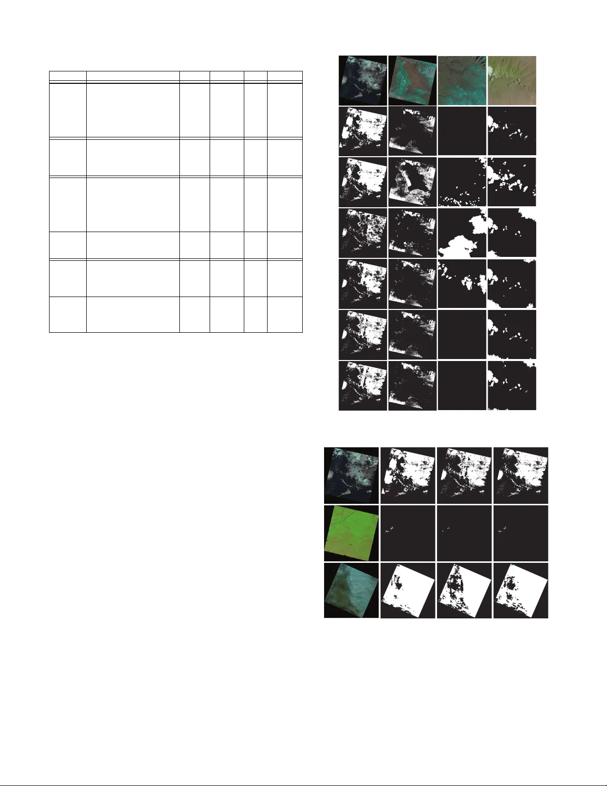
1 Cloud and Cloud Shado w Se gmentation for Remote Sensing Imagery via Filtered Jaccard Loss Function and P arametric Augmentation Sorour Mohajerani, Student Member , IEEE, Parv aneh Saeedi, Member , IEEE Abstract —Cloud and cloud shadow segmentation ar e fun- damental processes in optical r emote sensing image analysis. Current methods for cloud/shadow identification in geospatial imagery are not as accurate as they should, especially in the presence of snow and haze. This paper presents a deep learning- based framework for the detection of cloud/shadow in Landsat 8 images. Our method benefits from a convolutional neural network, Cloud-Net+ (a modification of our previously proposed Cloud-Net [1]) that is trained with a novel loss function (Filtered Jaccard Loss). The proposed loss function is more sensitive to the absence of f oreground objects in an image and penalizes/rewards the predicted mask more accurately than other common loss functions. In addition, a sunlight direction-awar e data augmen- tation technique is developed for the task of cloud shadow detection to extend the generalization ability of the proposed model by expanding existing training sets. The combination of Cloud-Net+, Filtered Jaccard Loss function, and the proposed augmentation algorithm delivers superior results on f our public cloud/shadow detection datasets. Our experiments on P ascal V OC dataset exemplifies the applicability and quality of our proposed network and loss function in other computer vision applications. Index T erms —Cloud detection, CNN, image segmentation, deep learning, Landsat 8, loss function, r emote sensing, 38-Cloud. I . I N T RO D U C T I O N C LOUD and cloud shadow detection, along with cloud cov erage estimation, are among the most critical pro- cesses in the analysis of remote sensing imagery . On the one hand, transferring remotely sensed data from air/space-borne sensors to ground stations is an expensi ve process from time, bandwidth, storage, and computational points of vie w . On the other hand, no useful information about the Earth’ s surface can be e xtracted from optical images that are heavily covered by clouds and their shadows. Since, on average, 67% of the Earth surface is cov ered by clouds at any giv en time [2], it seems that a considerable amount of resources can be saved by transferring only images with no/minimum amount of cloud and shado w cov erage. Cloud coverage by itself could provide useful information about climate and atmospheric parameters [3], as well as natural disasters such as hurricanes and volcanic eruptions [4], [5]. As a result, the identification of clouds and cloud shadows in images is an essential pre-processing task for many applications. Cloud and cloud shado w detection is ev en more challenging when only a limited number of spectral bands are av ailable. Many air/spaceborne systems such as ZY -3, HJ-1, S. Mohajerani and P . Saeedi are with the School of Engineering Sci- ence, Simon Fraser University , BC, Canada (e-mail: smohajer@sfu.ca, psaeedi@sfu.ca). and GF-2 are equipped only with visible and near-infrared bands [6]. Therefore, algorithms that can identify clouds and their shado ws from those few spectral bands become more essential. In recent years, many cloud/shadow detection algorithms hav e been developed. These methods can be divided into three main categories: threshold-based [7]–[10], handcrafted [11]– [14], and deep learning-based methods [15]–[20]. Function of mask (FMask) [21]–[23] and automated cloud- cov er assessment (A CCA) [24] algorithms are among the most well-known threshold-based algorithms for cloud identifica- tion. They construct a decision tree to label each pixel as cloud or other non-cloud classes. In each branch of the tree, a decision is made based on a thresholding function that utilizes one or more spectral bands of the data. A group of handcrafted methods isolated haze and thick clouds from other pixels using the relationship between spec- tral responses of the red and blue bands. Some examples of these algorithms include [25], [26], which are deriv ates of the Haze Optimized T ransformation (HO T) [11]. Xu et al. [27], proposed a handcrafted approach, which in volv ed a Bayesian probabilistic model incorporated with multiple spectral, temporal, and spatial features to separate cloud from non-cloud regions. W ith recent advances in deep-learning algorithms for image segmentation, se veral methods hav e been dev eloped to detect cloud/shadow using deep-learning. Xie et al. [19] trained a conv olutional neural network (CNN) from multiple small patches. Their network classified each patch into one of the three classes of thin cloud, thick cloud, and clear . A major issue in cloud/shadow detection approaches using deep- learning is the lack of accurately annotated training images since creating ground truths (GTs) for remote sensing imagery is time-consuming and tedious [28]. In addition, default cloud masks provided in remote sensing products are mostly ob- tained through automatic/semi-automatic thresholding-based approaches, which often make them less accurate. Authors in [29] have remov ed wrongly labeled icy/snowy regions in default cloud masks in their dataset. They sho wed that the performance of a well-known semantic segmentation model (U-Net [30]) is considerably improved by training on those corrected GTs. Although existing methods deliver promising results, many of them do not provide robust and accurate cloud/shadow masks in scenes where bright/cold non-cloud regions exist alongside clouds [15], [22]. Here, inspired by advances made in deep learning tech- niques, we propose a new algorithm to identify cloud/shadow 2 regions in Landsat 8 images. Our proposed algorithm consists of a fully con volutional neural network (FCN), which detects cloud and cloud shadow pixels in an end-to-end manner . Our network, Cloud-Net+, is a modified v ersion of our pre viously open-sourced model, Cloud-Net [1]. In the process of optimiz- ing Cloud-Net+ model, a nov el loss function named Filtered Jaccard Loss (FJL) is dev eloped and used to calculate the error . As a result, Cloud-Net+ is trained more accurately . FJL makes a considerable difference in the performance of systems, especially for images with no cloud/shadow regions. Many of the threshold-based and handcrafted algorithms for cloud shado w detection utilize geometrical relationships between the illumination source, clouds, and shado ws [21], [31], [32]. Ho wever , such relationships are not tak en adv antage of in deep learning-based approaches, where shadows are considered independent foreground objects. W e incorporate this information through a meaningful parametric data aug- mentation approach to have a greater variety of shadows in each scene. As a result, ne wly generated images resemble original images as if they were captured at different times of the day with dif ferent sunlight directions. Our experiments show that such systematic augmentation works very well for shadow detection and simultaneous multiclass segmentation of clouds, shado ws, and clear areas. Unlike FMask and ACCA, the proposed approach is not blind to the existing global and local cloud/shado w features of an image. Also, since only four spectral bands—red, green, blue, and near-infrared (RGBNir)—are required for the system’ s training and prediction, the proposed method can be easily utilized for images obtained by most of the existing satellites as well as airborne systems. Unlike multitemporal- based methods such as [33], the proposed method does not require prior kno wledge of the scene, e.g., cloud-free images. The only data required for the parametric augmentation are solar angles, which exist in the metadata accompanying each image. Moreover , such information is used for training pur- poses only and not for prediction. In addition, to being simple and straightforward, the proposed network can be used in other image segmentation applications. In summary , the contrib utions of this work are as follo ws: • Proposing a nov el loss function (FJL), which not only penalizes a model for poor prediction of clouds and shadows but also fairly re wards the correct prediction of clear re gions. Our e xperiments sho w that FJL outperforms other commonly used loss functions. In addition, when Cloud-Net+ is trained with it, its results outperform state-of-the-art cloud/shadow detection methods o ver four public datasets of 38-Cloud, 95-Cloud, Biome 8, and SP ARCS. • Proposing a Sunlight Direction-A ware Augmentation (SD AA) technique to boost the shadow detection per- formance. Unlike commonly used transformation-based augmentation techniques such as rotation and flipping, which are blind to the scene’ s geometry , SD AA generates synthetic shado ws with various lengths, directions, and lev els of shade. • Extending our public dataset, 38-Cloud [1], for cloud de- tection in Landsat 8 imagery to a new dataset (95-Cloud). This ne w dataset—which is made public—includes 57 more Landsat 8 scenes (than 38-Cloud) along with their manually annotated GTs. It will help researchers improve their cloud detection algorithms using more training and ev aluation data. The remainder of this paper is organized as follows: in Section II, a summary of related works in the cloud detection field is revie wed. In Section III, our proposed method is explained. In Section IV , experimental results are discussed. Finally , Section V summarizes our work. I I . R E L A T E D W O R K S Cloud and shado w detection in remotely sensed images ha ve been an activ e area of research for many years. One of the first attempts to distinguish between clouds and cloud-free areas was through a probabilistic classifier model [34]. Ho wev er , it was limited to scenes with clouds ov er open sea surfaces. One of the first successful and more general automatic cloud detection methods was Fmask (first version) [21]. Fmask used sev en bands of Landsat images to classify each pixel of an image into one of the fi ve classes of land, water , cloud, shado w , and snow . Another version of it (Fmask V3) [22] utilized cirrus band to distinguish cirrus clouds along with low altitude clouds. In the last version of it (Fmask V4) [23], auxiliary data such as digital elev ation maps (DEM), DEM deri vati ves, and global surface water occurrences (GSWO) were used in addition to the other usual bands for better performance on water , high altitude regions, and Sentinel-2 images. Sev eral multitemporal methods were developed for cloud/shadow detection [27], [35]–[37]. Mateo-Garc ´ ıa et al. [33] used cloud-free images of Landsat 8 scenes to identify potential clouds. A clustering and some threshold-based post- processing steps then helped to generate final cloud masks. Zi et al. [38] combined a threshold-based method with a classical machine learning approach to segment superpixels and classify them into one of three classes of cloud, potential cloud, and non-cloud. Recently , sev eral FCNs hav e been developed for cloud and cloud shadow detection tasks [28], [39]–[43]. Y ang et al. [44] proposed an FCN, which detects clouds in ZY -3 thumbnail satellite images. A b uilt-in boundary refinement approach was incorporated into their network (CDnetV1) to av oid further post-processing. The second version of that network, CDnetV2 [45], was equipped with two ne w feature fusion and information guidance modules to extract cloud features more accurately . Chai et al. [46] proposed Segnet Adaption (a modified version of a well-kno wn FCN for semantic segmentation) to match with remotely sensed images. Segnet Adaption has shown promising results on Biome 8 and Landsat 7 cloud/shadow detection datasets. Recently , Jeppesen et al. [47] introduced RS-Net to identify clouds in Landsat 8 images. RS-Net was an FCN inspired by U-Net and was trained with both automatically (via Fmask) and manually generated GT images of two public datasets. The authors showed that results obtained by a model trained with Fmask’ s outputs outperform the Fmask directly obtained results. The authors of SP ARCS CNN [48] also proposed a model to distinguish cloud, shado w , water , snow , and clear regions 3 in Landsat 8 images. They used a pretrained VGG16 as the backbone of their fully con volutional network. The y succeeded in reaching human interpreter accuracy with their model. Re- fUnet v1 [49] was another method which focuses on retrieving fuzzy boundaries of clouds and shadows. The authors used a UNet for extracting course/rough cloud and cloud shadow in small patches of images. Then, boundaries of clouds/shadows in complete Landsat 8 masks were refined/sharpened using a dense conditional random field (CRF). In this method, the CRF refinement was applied as a post-processing step. In the second v ersion of RefUNet (RefUNet v2) [50] a simultaneous joint pipeline for detecting and refining edges was utilized. Therefore, the UNet network, which identified course masks, was concatenated with the proposed Guided Gaussian filter- based CRF to refine boundaries in an end-to-end manner . In addition, refinements were done on small patch masks rather than large masks of the entire Landsat 8 scenes. In another work, the authors of Cloud-AttU [51] employed a UNet model that is enriched with a specific attention module in its skip connections. Multiple attention modules enabled the model to learn proper features by paying attention to the most rele vant locations in input training images or feature maps. CloudFCN [52] was based on a UNet model with the addition of inception modules between con volution blocks in the contracting and expanding arms. In addition to pix el-lev el segmentation, the authors incorporated a feature into their algorithm for estimating cloud coverage in an image using a regression-friendly loss function. They demonstrated that CloudFCN could achie ve high accuracy in the task of cloud screening under various conditions, such as the presence of white noise and using dif ferent quantization methods. Image augmentation has been prov en to be effecti ve in increasing the accuracy of deep learning models. There are only a fe w offline augmentation algorithms reported for re- mote sensing imagery . Ma et al. [53] proposed a generati ve adversarial network (GAN) to synthesize images for scene labeling. Howe et al. [54] introduced another GAN-based approach for Earth’ s surface object detection in airborne images. Zheng et al. [55] proposed a method for generating synthetic vehicles in aerial images. For the specific task of cloud/shadow segmentation, only basic geometric and color space transformations in the training phase are used for data augmentation [16], [56]. Authors of [57], howe ver , developed a GAN (CloudMaskGAN) to con vert snowy scenes to non- snowy and vice versa for augmentation of Landsat 8 images. T o the best of our knowledge, CloudMaskGAN is the only reported non-transformation-based augmentation approach for cloud detection purposes. I I I . P RO P O S E D M E T H O D In this section, the proposed methodology for cloud/shadow detection is described. W e focus on using Landsat 8 images. Landsat 8 is equipped with two optical sensors, which together collect eight spectral and tw o thermal bands. Only four spectral bands—Bands 2 to 5 (RGBNir)—are used (all with 30 m spatial resolution). T o keep the proposed method more general, no thermal band is utilized. A. Arc hitectur e of the Se gmentation Model Similar to other FCNs, the proposed network is made of two main arms: a contracting arm, and an expanding arm. In the training phase, the contracting arm extracts important high-lev el cloud/shadow attributes. It also do wnsamples the input while increasing its depth. On the other hand, the expanding arm utilizes those extracted features to build an image mask—with the same size as the input. The network’ s input is a multi-spectral image, and its output is a grayscale cloud/shadow probability map for the input. In the case of multiclass segmentation, the output has multiple channels, one corresponding to each class. W e modified the network’ s architecture in our previous work [1] to de velop a more ef ficient model that is more sensiti ve to clouds/shadows. Cloud-Net+, consists of six contracting and fiv e expanding blocks (see Fig.1). Successive conv olutional layers are the heart of the blocks in both arms. The kernel size and the order of these layers play crucial roles in the quality of activ ated features, and therefore, they affect the final segmentation outcome directly . On the one hand, it seems that as the number of con volutional layers in each block increases, the distinction of the captured context improv es. On the other hand, utilizing more of such layers explodes the complexity of the model. T o address such trade-off, we remove the middle 3 × 3 con volution layer in the last two contracting blocks and the first expanding block of Cloud-Net. Since those layers are dense and contain thousands of parameters, such remo val decreases the number of network’ s parameters significantly . Then, in all contracting arm blocks, a 1 × 1 conv olution layer is added between each two adjacent 3 × 3 con volution layers. Since each 1 × 1 conv olution layer contains a small number of parameters, the total number of parameters of Cloud-Net+ ( 32 . 9 M) is 10% less than that of Cloud-Net ( 36 . 4 M). Utilizing the 1 × 1 kernel size in con volutional layers was suggested initially in [58], and its effecti veness is proven in works such as [59]. Employing such a kernel in expanding blocks does not yield a better recovery of the lo w-resolution feature maps. Therefore, we do not add it to the e xpanding blocks. Instead, an aggreg ation branch (AB) is added to combine all feature maps of the expanding blocks. AB consists of six up-sampling layers (bilinear interpolation) follo wed by a 1 × 1 con volution. It helps our model to retrie ve cloud/shadow boundaries in the generated masks. B. Loss Function Soft Jaccard/Dice loss function has been widely used to optimize many image segmentation models [60]–[62]. The formulation of soft Jaccard loss for two classes of ” 0 ” and ” 1 ” is as follo ws: J L ( t, y ) = 1 − N P i =1 t i y i +  N P i =1 t i + N P i =1 y i − N P i =1 t i y i +  , (1) Here t represents the GT , and y is the output of the network. N denotes the total number of pixels in t . y i ∈ [0 , 1] and t i ∈ { 0 , 1 } are the i th pixel value of y and t , respectiv ely , and  is 10 − 7 to av oid division by zero. Soft Jaccard loss function, ho wev er , has a defect: over -penalization of images with no class ” 1 ” in their GTs. 4 FF Block FF Block Up Block Up Block FF Block FF Block FF Block Contr . Block Contr . Block Contr . Block Contr . Block Contr . Block Exp. Block Exp. Block Exp. Block Exp. Block Exp. Block Up Block Up Block Up Block Up Block Contr . Block Conv . (3x3) Conv . (3x3) Conv . (1x1) Conv. (1x1) M C Contr . Block Contr. Block FF Block FF Block Upsampling Block Exp. Block C M U Concatenation Maxpooling Up-sample Addition Conv . T C Conv . (3x3) Conv . (3x3) U Conv . (1x1) C C M M x 1 : input of the i th FF block x i+1 x i x i FF: Feedforward Contr .: Contracting Exp.: Expanding Fig. 1: Cloud-Net+’ s architecture. Let us consider a small 2 × 2 input image with t 0 = [0 , 0; 0 , 0] and two possible predictions of y 1 = [0 . 01 , 0 . 01; 0 . 01 , 0 . 01] and y 2 = [0 . 99 , 0 . 99; 0 . 99 , 0 . 99] . It is clear that y 1 would be a better prediction than y 2 since it can be interpreted as having no class ” 1 ” in the input image. Howe ver , soft Jaccard losses obtained by y 1 and y 2 are the same: J L ( t 0 , y 1 ) = J L ( t 0 , y 2 ) ≈ 1 . Consequently , the network penalizes y 1 as much as y 2 , even though y 1 represents a better prediction. Indeed, the major problem with soft Jaccard loss function is that whenever there is no class ” 1 ” in the GT , the numerator of Eq. (1) equals to  (which is a small number) and, as a result, the v alue of the loss approximates 1 . Observing this behavior , we propose a modified soft Jaccard loss function, FJL, with two different v ersions. The main idea behind FJL is to compensate for unfair v alues of soft Jaccard loss and replace them with proper values whenev er there is no class ” 1 ” in the GT . W e can summarize the goal of the FJL as follo ws: FJL ( t, y ) = ( G L ( t, y ) , t i = 0 , ∀ i ∈ { 1 , 2 , 3 , ...,N } J L ( t, y ) , O therw ise (2) where G L represents a compensatory function. The condition in the first line of Eq. (2) indicates that when all pixels of GT are equal to zero, FJL is similar G L . Clearly , this condition can be rephrased as follo ws: FJL ( t, y ) = ( G L ( t, y ) , S = 0 J L ( t, y ) , S > 0 (3) where S = P N i =1 t i . This formulation can be re written—in a more general form—as the combination of two functions of J L and G L , in which each function is multiplied by ideal highpass and lo wpass filters, respecti vely: FJL ( t, y ) = k G G L ( t, y ) LP p c ( S ) + k J J L ( t, y ) H P p 0 c ( S ) (4) Here, LP p c denotes a lo wpass filter with the cut-of f point of p c and H P p 0 c denotes a highpass filter with the cut-off point of p 0 c . k G and k J represent coefficients of compensatory and Jaccard losses, respectiv ely . The magnitude of both filters is limited in the [0,1] range. In Eq. (4), the value of LP p c is 0 when S > p c , so the value of G L ( t, y ) LP p c becomes zero, and as a result, FJL only has contributions from J L . On the other hand, when S < p 0 c , H P p 0 c becomes 0 , and FJL is only from the G L part. This behavior can be simply described as a toggle switch between J L and G L . T o satisfy Eq. (3), the cut-off point of the two ideal filters should be equal, so they become complementary . Note that, in signal processing context, the cut-of f usually refers to the ”frequency” at which the magnitude of a filter changes. Howe ver , in this work, cut-of f is the ”v alue” of S at which the magnitude of a filter alters. Since this transition should occur when S = 0 , the cut-off points are set to 0 . T o have lo wpass and highpass filters with smooth gradient characteristics, inspiring by [63], we hav e used the sigmoid function as follo ws: L P p c ( S ) = 1 1 + exp  m ( S − p c )  , H P p 0 c ( S ) = 1 1 + exp  m ( − S + p 0 c )  (5) where m denotes the steepness of the sigmoid transition. Choosing sigmoid solv es the problem of over -penalizing without adding any non-differentiable elements or piecewise conditions to the loss function. This leads to a smooth switch between soft Jaccard and compensatory loss in FJL. Since H P and LP filters are not functions of y , the gradient of FJL is still continuous (without any jumps). By substituting Eq. (5) in Eq. (4), FJL is described as: FJL ( t, y ) = k G G L ( t, y ) 1 + exp  m ( S − p c )  + k J J L ( t, y ) 1 + exp  m ( − S + p 0 c )  (6) T o keep these filters close to ideal, m is required to be a large number . W e hav e set m to 1000 in our experiments to hav e fast transitions from 0 to 1 and vice versa. In addition, p c and p 0 c are set to 0 . 5 to leave a safety margin and ensure that LP 0 . 5 ( S = 0)= 1 and H P 0 . 5 ( S = 0)= 0 . Also, by setting k G = k J = 1 , the magnitude of the loss remains in [0 , 1] range. W e can have dif ferent versions of FJL, by selecting different functions as G L . Here, we in vestigate two dif ferent candidates, G L 1 and G L 2 , to form two corresponding FJL versions, FJ L 1 and FJ L 2 . Our first candidate is the in verted Jaccard function, which is calculated by the complements of GT and prediction arrays. The second one is the normalized version of a common loss function in segmentation tasks, Cross Entropy (CE). The formulation of these candidates are as follows: G L 1 ( t, y ) ≡ I nv J L ( t, y ) = J L ( t, y ) , (7) G L 2 ( t, y ) ≡ C E norm ( t, y ) = C E ( t, y ) M ax = − 1 N N P i =1  t i log ( y i +  )  M ax , where t and y denote the complements of t and y , respec- tiv ely . C E norm denotes normalized CE. T o make sure that the range of FJ L 2 ( t, y ) is bounded to [0 , 1] , CE values are normalized by division by their maximum possible value, 5 M ax = − N N log(  ) = 16 . 1180 . M ax is obtained when all pixels in the predicted array are complements of GT . C. P arametric Augmentation (SD AA) When an image is captured by Landsat 8, the solar azimuth ( θ A ) and the zenith ( θ Z ) angles at the time of acquisition are recorded in a metadata file. W e use these angles to generate different synthetic images by hypothetically changing the sun’ s location in the sky and, therefore, creating shado ws under different illumination directions. This could be interpreted as capturing the same scene at different times of the day . Each image can be augmented unless it is free of shadow . The main steps of the proposed SD AA are as follows: 1) removing original shadows, 2) changing the direction of illumination, 3) generating the locations of synthetic shadows by projecting clouds using the synthetic illumination direction of step 2, 4) recoloring synthetic shadow locations to generate different le vels of shades via gamma transformation. Details of these steps are e xplained next. First, a Landsat 8 image (from the training set), its shado w GT , and its cloud GT are selected. T o generate realistic images, original shadows should be removed from the image, other- wise, the synthetic image will hav e two cast shado ws. For the shadow remo val step, a histogram matching between shadow regions and their shadow-free neighborhood is performed. The result of this step is a shadow-free image. Original False-color GT Augmented Image Augmented GT θ Α Ο = 90, r = 100, γ = 0.95 θ Α Ο = 180, r = 60, γ = 0.875 θ Α Ο = 270, r = 80, γ = 0.80 Fig. 2: Examples of SD AA obtained from one of the SP ARCS images. The yellow arro w shows the sunlight direction in each image. T o create new shado ws in the shadow-free image, we gener- ate synthetic solar angles by adding offsets to the original solar angles of θ A and θ Z . Using these new angles, the direction of synthetic sunlight (in form of a 2 D vector projected on the scene’ s image plane) is calculated. By moving cloud pixels on the image plane and in the direction of the ne w sunlight, synthetic shadows of those clouds are generated. W e made the following assumptions to simplify this process: all clouds have the same height, and the scene is located on a flat plane. The following equations are used to obtain the new locations of the cast shado ws: y sh = y cl + r sin( θ Z + θ Z O ) cos( θ A + θ A O ) , x sh = x cl + r sin( θ Z + θ Z O ) sin( θ A + θ A O ) , (8) where y cl , y sh , x cl , and x sh denote the location of a cloud pixel and its corresponding cast shado w along the y and x axes. θ Z O and θ A O represent solar angle offsets. r (in pixels) is the shifting f actor , which defines the length of a cast shado w . The greater the r is set, the more a piece of cloud is shifted, and therefore, the longer its shadow becomes. Since both r and θ Z could affect the length of the cast shadow , instead of altering both, we keep θ Z intact and only alter r . Therefore, θ Z O is set to 0 . The resultant synthetic shadow mask (SSM) will be used as the shadow GT of the augmented image in the training phase. In the next step, SSM is used to adjust the brightness of the synthetic shadow regions in the augmented image using gamma ( γ ) transformation ( i 0 = i γ ). Pixel values of shadow- free regions in the image—including cloudy and clear areas— are not modified. Multiple candidates have been considered for hyperparam- eters of SD AA: θ A O , r , and γ . These candidates consist of: θ A O = { 90 , 180 , 270 } ◦ , r = { 20 , 40 , 60 , 80 , 100 } , and γ = { 0 . 8 , 0 . 825 , 0 . 85 , 0 . 875 , 0 . 9 , 0 . 925 , 0 . 95 , 0 . 975 } . Note that θ A O is selected to cov er all possible ranges of the solar azimuth angle— [0 , 360] . V alues of r greater than 100 generate too long and unrealistic shadows. In addition, choosing γ values smaller than 0 . 8 and greater than 0 . 975 leads to too dark and unnatural-looking bright shadows. The entire process is repeated for all spectral bands (R, G, B, and Nir). Fig. 2 displays some of the augmented images generated by SD AA. I V . E X P E R I M E N TA L S E T T I N G S A N D R E S U LT S A. T raining Details The size of the input data for Cloud-Net+ is 192 × 192 × 4 . Four spectral bands of each patch are stacked up in the following order: R, G, B, Nir , to create such input. Before training, input patches are normalized through division by 65535. 20% of training data is used for v alidation during the training. Input patches are randomly augmented using simple online geometric translations such as horizontal flipping, rotation, and zooming. Note that to make the proposed loss functions compatible with multiclass segmentation e xperiments, in each iteration of the training, loss values obtained for each class are averaged (with weights proportional to the in verse number of pixels in each class). The acti vation function in the last con volution layer of the network is a sigmoid. In the case of multiclass segmentation, softmax function is used in the last layer . Adam method [64] is utilized as the optimizer . The initial weights of the network are obtained by a Xavier uniform random initializer [65]. The initial learning rate for the model’ s training is set to 10 − 4 . If the v alidation loss does not drop for more than 15 successiv e epochs, the learning rate is reduced by 70% . This policy is continued until the learning rate reaches 10 − 8 . The batch size is set to 12 . The proposed network is dev eloped using Keras deep learning framework with a single GPU. B. Datasets 1) 38-Cloud Dataset: 38-Cloud dataset, which has been introduced in [1], consists of 8400 non-overlapping (NOL) patches of 384 × 384 pixels extracted from 18 Landsat 8 Collection 1 Lev el-1 scenes as the training set. 9201 patches of the same spatial size obtained from 20 Landsat 8 scenes 6 represent the test set. Scenes are mainly from North America and their GTs are manually extracted. This dataset includes only four spectral bands of R, G, B, and Nir . All Landsat 8 scenes have black (empty) regions around them. These regions are created when the acquired images are aligned to ha ve the geodetic north at their top. W e eliminated training patches with more than 80% empty pixels. The number of non-empty training patches decreases to 5155 , resulting in a significant decrease in training time. 2) 95-Cloud Dataset: T o improve the generalization ability of deep neural networks trained on 38-Cloud dataset, we hav e extended it by adding 57 new Landsat 8 scenes to the training scenes of 38-Cloud dataset. Therefore, in total, the new training set consists of 75 scenes. 38-Cloud test set has been kept intact in 95-Cloud dataset for e valuation consistenc y . The GTs for the ne w scenes are manually extracted. Dif ferent images in 95-Cloud are selected to include v arious land cov er types such as soil, ve getation, urban areas, snow , ice, water , haze, and different cloud patterns. The av erage cloud cov erage percentage in 95-Cloud dataset images is k ept around 50% . Following the same pattern as in 38-Cloud dataset, the total number of patches for training is 34701 and for the test is 9201 . Removing empty patches from 95-Cloud training set reduces the number of patches to 21502 . W e made this dataset and parts of the code publicly av ailable to the community at https://github .com/SorourMo/95-Cloud-An- Extension-to-38-Cloud-Dataset . 3) Biome 8 Dataset: Biome 8 dataset [66] is a publicly av ailable dataset consisting of 96 Landsat 8 scenes with their manually generated GTs with fi ve classes of cloud, thin cloud, clear , cloud shado w , and empty . W e generated a binary cloud GT out of Biome 8 GTs by merging both thin cloud and cloud classes into one cloud class. W e marked the rest of the classes as clear . For the shado w segmentation task, all classes, except shadow , are combined under a clear class. Follo wing the same pattern from 38-Cloud and 95-Cloud datasets, the total number of cropped patches e xtracted from the entire Biome 8 dataset is 44327 . Removing empty patches reduces this number to 27358 . 4) SP ARCS Dataset: SP ARCS dataset [48], [67] consists of 80 patches of 1000 × 1000 extracted from complete Landsat 8 scenes. The GTs of these patches are manually generated. Each pix el is classified into one of the cloud, shadow , sno w/ice, water , land, and flooded classes. For the binary segmentation of clouds/shadows, we have combined all non-cloud and non- shadow classes under the clear class. In multiclass segmenta- tion, three classes of cloud, shado w , and clear have been kept. Follo wing the same pattern as previous datasets, the number of extracted NOL patches for this dataset is 720 . C. Model Evaluation T o e valuate the performance of the proposed algorithm, various experiments are performed. For 38-Cloud and 95- Cloud datasets, our model is trained and tested on each of those datasets’ explicitly defined training set and testing set, respectiv ely . For SP ARCS dataset, as suggested in [47], we randomly extract five folds of images (each fold consists of 16 complete images or 144 NOL patches). Folds 2 to 5 are considered for training and fold 1 for testing in our experiments. W e have also conducted 5-fold cross-validation (5CV) over the extracted folds to compare obtained results with those from RS-Net [47]. For Biome 8 dataset, we follow the instructions described in [47] and extract two folds from Biome 8 dataset. W e randomly select two cloudy , two mid-cloud, and two clear scenes for each biome category . Therefore, 48 scenes are extracted for fold 1 and 48 scenes for fold 2. In our experiments, fold 2 is used for training and fold 1 for testing. T o compare against RS-Net, 2-fold cross-validation (2CV) is conducted, and the obtained numerical results are a veraged. Evaluation of the SDAA method requires different arrange- ments. For SP ARCS, multiple sets of augmented training images are generated using v arious combinations of hyperpa- rameters described in section III-C. NOL patches of 384 × 384 pixels are extracted from those images and are added to the original training patches of SP ARCS dataset one set at a time. Then, to find the best combination of hyperparameters, shadow detection training and testing are performed for each of those expanded training sets. The numerical results of these experiments are calculated and compared against those obtained from training with original patches only . Those com- binations of hyperparameters that resulted in a higher Jaccard index than the training with original patches are identified (11 combinations). SD AA patches are generated by those combinations and added all together to the original training patches of a dataset for a final ev aluation. Considering SP ARCS’ s folds 2 to 5 as the training set, we use the best hyperparameters confirmed in the previous steps to generate SDAA patches, leading to 6812 training patches in total. F or Biome 8 dataset, we consider 70% of the patches (extracted from 32 scenes with shadow) for training and the rest for testing to hav e a fair comparison against Segnet Adaption [46]. Generating SD AA patches for this training set and then adding them to the original training patches results in 17155 patches in total. After training the proposed model with training patches of the abov e-mentioned datasets, the obtained weights are sav ed and used for the ev aluation of the model by prediction over unseen test scenes. T est patches of each scene are resized to 384 × 384 × 4 and fed to the model. Then, the cloud/shado w probability map corresponding to each patch is generated. Next, probability maps (grayscale images) are stitched together to build a prediction map for a complete scene. A 50% threshold is used to get a final binary mask. In multiclass segmentation, an ar g max operation is applied on the output probability map to produce a mask for each class. Cloud prediction by Cloud-Net+ takes about 30 s for all patches of a typical Landsat 8 scene with a P100-PCIE-12GB GPU, half of which is for reading and preparing, and the other half is for inference. D. Evaluation Metrics Once cloud masks of complete Landsat 8 scenes (including empty patches) are obtained by our algorithm, they are com- pared against their corresponding GTs. Then, the performance is quantitativ ely measured by Jaccard index (or mean Intersec- tion o ver Union (mIoU)), precision, recall, and accuracy . These 7 metrics are commonly used in state-of-the-art segmentation algorithms and are defined as follows: Jaccard Index = P M i =1 tp i P M i =1 ( tp i + f p i + f n i ) , Precision = P M i =1 tp i P M i =1 ( tp i + f p i ) , Recall = P M i =1 tp i P M i =1 ( tp i + f n i ) , Accurac y = P M i =1 ( tp i + tn i ) P M i =1 ( tp i + tn i + f p i + f n i ) , where tp , tn , f p , and f n are the numbers of true positiv e, true negati ve, false positi ve, and false neg ativ e pixels for each class in each test set scene. M is the total number of scenes in the test data. E. Quantitative and Qualitative Results 1) Evaluation of the Pr oposed Loss Functions: T able I demonstrates experimental results for e valuating the proposed loss functions. From T able I, we conclude that for both 38- Cloud and SP ARCS datasets, Cloud-Net+ trained with both versions of FJL performs better than the original loss functions that they are deriv ed from. A comparison of different loss functions over 38-Cloud dataset is displayed in Fig. 3. Note the better performance of both FJL loss functions on detecting thick and thin clouds (haze) over snow (two middle columns). T ABLE I: Quantitative results for the proposed loss functions obtained by Cloud-Net+ model for cloud detection (in %). T raining/T est Loss Jaccard Precision Recall Accuracy 38-Cloud training set /test set J L 88.41 97.44 90.51 96.21 proposed FJ L 1 88.85 97.39 91.01 96.35 C E 87.71 97.25 89.94 95.97 proposed FJ L 2 88.26 97.70 90.13 95.91 SP ARCS folds 2-5 /fold 1 J L 81.77 92.78 87.32 94.69 proposed FJ L 1 83.99 92.23 90.37 95.30 C E 81.55 92.25 87.55 94.60 proposed FJ L 2 85.11 93.43 90.52 95.68 2) Evaluation of the Pr oposed SD AA Method: Numerical results for cloud shadow detection with and without SD AA using dif ferent loss functions are reported in T able II. From this table, the addition of the augmented patches obtained by SD AA improves all ev aluation metrics over SP ARCS dataset compared to using original training patches only . Using SD AA to train ov er Biome 8 dataset also results in a higher Jaccard index and accuracy than without it. T ABLE II: Quantitative results of shadow detection using SDAA obtained with Cloud-Net+ and different loss functions (in %). T raining/T est Loss Jaccard Precision Recall Accuracy SP ARCS folds 2-5 / fold 1 J L 58.99 76.82 71.76 95.97 C E 57.55 79.06 67.90 95.95 proposed FJ L 1 60.59 75.09 75.84 96.02 proposed FJ L 2 60.52 74.91 75.91 96.00 SP ARCS folds 2-5 + SDAA patches / fold 1 J L 62.38 79.05 74.73 96.36 C E 61.66 81.09 72.01 96.38 proposed FJ L 1 63.44 79.20 76.12 96.45 proposed FJ L 2 63.22 78.41 76.54 96.40 Biome 8 70% / 30% proposed FJ L 1 53.79 58.45 87.09 98.21 proposed FJ L 2 52.11 56.31 87.47 98.07 Biome 8 70%+SD AA / 30% proposed FJ L 1 54.71 64.05 78.94 98.43 proposed FJ L 2 54.41 59.67 86.06 98.27 3) Comparison with State-of-the-art Cloud Detection Meth- ods: T able III compares cloud detection results obtained by the proposed method with other methods on various datasets. From this table, the combination of the proposed Cloud-Net+ False-color Ground truth Cloud-Net+ Loss = J L Cloud-Net+ Loss = CE Cloud-Net+ Loss =FJL 1 Cloud-Net+ Loss =FJL 2 Fig. 3: V isual examples of the cloud detection results over patches of 38- Cloud test set obtained by different loss functions. with F J L 1 deliv ers a higher Jaccard index over 38-Cloud dataset than the U-Net, Cloud-AttU, and Fmask V3 methods. Four visual examples of the predicted cloud masks are displayed in Fig. 4. The second and third columns show scenes in the presence of snow . Fmask and U-Net call many f p s where land is covered with snow . The image of the third column does not include any clouds. The only method that successfully identifies all clear pixels is our method. The fourth column of this figure is captured over a region with bare soil—another difficult case for detecting clouds. The proposed method can distinguish those regions from clouds more accurate than the other methods. Although it is not fair to compare our method (which only uses four spectral bands) with Fmask V4 (which uses sev en spectral bands, one thermal band, DEM, and GSWO), we obtained the numerical results of Fmask V4 over 38- Cloud test set. Fmask V4 shows lower accuracy ( 96 . 23% ) compared to Cloud-Net+ with F J L 1 . Note that Fmask V4 has limited applicability , as not many remote sensing platforms are equipped with more than four spectral bands of RGBNir . The numerical results over 95-Cloud test set (which has the same test set as 38-Cloud) are improved since they are obtained by a network trained with more training images (95- Cloud training set is larger than 38-Cloud). Fig. 5 highlights the improv ement of results o ver this dataset. For SP ARCS dataset, Cloud-Net+ outperforms SegNet [68] and PSPNet [69], two common semantic segmentation meth- ods. In addition, Cloud-Net+ outperforms RS-Net over two datasets of SP ARCS and Biome 8. On Biome 8 dataset, our 8 T ABLE III: Comparison of the proposed cloud detection method with other methods (in %). T rain/T est Method Jaccard Precision Recall Accuracy 38-Cloud training set /test set Fmask V3 [22] 85.91 88.65 96.52 94.94 U-Net [29] 85.03 96.15 88.02 95.05 Cloud-Net [1] 87.32 97.60 89.23 95.86 Cloud-AttU [51] 88.72 97.16 91.30 97.05 Cloud-Net+ + FJ L 1 (ours) 88.85 97.39 91.01 96.35 Cloud-Net+ + FJ L 2 (ours) 88.26 97.70 90.13 95.91 95-Cloud training set /test set Fmask V3 [22] 85.91 88.65 96.52 94.94 Cloud-Net [1] 90.83 97.67 92.84 97.00 Cloud-Net+ + FJ L 1 (ours) 91.57 96.94 94.28 97.23 Cloud-Net+ + FJ L 2 (ours) 91.01 97.49 93.19 97.06 SP ARCS folds 2-5 /fold 1 Fmask V3 [22] 73.01 78.37 91.44 90.79 SegNet [68] 75.80 83.35 89.33 92.23 PSPNet [69] 78.91 90.11 86.39 93.71 Cloud-Net [1] 81.36 90.81 88.66 94.46 Cloud-Net+ + FJ L 1 (ours) 84.00 92.23 90.37 95.30 Cloud-Net+ + FJ L 2 (ours) 85.11 93.43 90.52 95.68 SP ARCS 5CV RS-Net [47] - 88.92 83.89 94.85 Cloud-Net+ + FJ L 1 (ours) 83.11 90.75 90.82 96.20 Cloud-Net+ + FJ L 2 (ours) 83.14 90.77 90.81 96.23 Biome 8 fold 2 /fold 1 Fmask V3 [22] 79.81 82.38 96.24 93.05 Cloud-Net [1] 84.84 93.92 89.78 95.48 Cloud-Net+ + FJ L 1 (ours) 85.44 92.88 91.42 95.55 Cloud-Net+ + FJ L 2 (ours) 85.15 91.43 92.52 95.39 Biome 8 2CV CloudFCN [52] - - 90.57 91.00 RS-Net [47] - 92.15 91.31 92.10 Cloud-Net+ + FJ L 1 (ours) 85.15 90.80 93.28 95.27 Cloud-Net+ + FJ L 2 (ours) 83.71 88.69 93.79 94.67 method, which utilizes only four spectral bands, shows a higher recall and accuracy than that of CloudFCN that uses elev en spectral bands. Note that Jaccard index and accuracy take into account both f p and f n in a predicted mask and penalize for all of those falsely labeled pixels, as opposed to precision and recall, which only penalize for one of the f p and f n . That is why Jaccard index—which is not reported in some papers—and accuracy are the most important metrics when one judges different methods. V isual results over Biome 8 dataset are sho wn in Fig. 6. 4) Comparison with State-of-the-art Cloud and Shadow Detection Methods: The numerical results for simultaneous segmentation of cloud, shado w , and clear regions ov er two datasets are reported in T able IV. The reported A verage Jaccard in this table is the av erage of Jaccard indices over three classes. T wo settings were considered for e v aluation by the authors of SP ARCS CNN: a) using 72 images from the SP ARCS dataset for training and the rest of SP ARCS images for testing, and b) utilizing the same 72 SP ARCS images for training and 24 scenes from the Biome 8 dataset for testing (names of these 24 scenes are listed in [48]). W e used the same settings in our experiments for a fair comparison. T wo pixels were considered by the authors of CNN SP ARCS as a leew ay buf fer at boundaries of predicted clouds and shadows and clear regions, where either class was considered correct within two pixels from the predicted boundary in ground truths. Note that we used no b uffer pixels for the e valuation of our method. According to T able IV, when SP ARCS CNN is trained on SP ARCS dataset and ev aluated on Biome 8 (even by considering a two-pixel buf fer), it is outperformed by our method in terms of accuracy . Ho wev er, when this method is trained and ev aluated on SP ARCS dataset, the numerical results are almost perfect. It should be noted that those perfect False-color Ground truth Cloud-Net [1] U-Net [29] Cloud-Net+ Loss=FJL 1 Fmask [22] Cloud-Net+ Loss=FJL 2 Fig. 4: V isual examples of cloud detection over 38-Cloud dataset. False-color Ground truth Cloud-Net+ Trained on 38-Cloud Cloud-Net+ Trained on 95-Cloud Fig. 5: V isual examples of cloud detection over 95-Cloud dataset. results reported for this experiment are obtained by having a two-pixel leeway buffer and using ten spectral bands, as opposed to no lee way b uffer and using only four spectral bands in our method. As an example of how much this two-pixel leew ay affects numerical results of the SP ARCS CNN, notice the improvement in accuracy (from 91.04% to 95.4%), where SP ARCS CNN method is trained on the SP ARCS dataset and ev aluated on the Biome 8. Fig. 7 displays some visual results 9 False-color Ground truth Fmask [15] Cloud-Net+, Loss=FJL 1 Fig. 6: V isual examples of cloud detection over Biome 8 dataset. for simultaneous segmentation of clouds and cloud shadows ov er SP ARCS dataset. For comparison againt RefUNets, we downloaded the cited the training, v alidation, and testing Landsat 8 scenes and con- ducted our experiments on them. In RefUNet v1 and RefUnet v2, the input consists of four (RGBNir) and sev en spectral bands, respectiv ely , while the default cloud and shadow masks extracted from Landsat 8 products’ QA bands are used for ground truths in e xperiments. Although sophisticated boundary refinements were applied on RefUnet methods’ s output masks, the obtained accuracy by either of these methods is not as high as the proposed method. False-color Ground truth Cloud-Net [1] Proposed Cloud-Net+ +SDAA, Loss=FJL 2 Fmask [23] Fig. 7: V isual examples of cloud and shado w detection results over SP ARCS dataset. White and gray pixels sho w cloud and shado w regions. T ABLE IV: Quantitati ve results for simultaneous cloud and shadow detection (in %). In columns 2 to 4, the first row indicates metrics for the cloud class, the second row for the shadow class, and the third row for the clear class. T raining/ T est Model Jaccard Precision Recall A verage Jaccard Accuracy SP ARCS folds 2-5 /fold 1 Fmask V3 [22] 73.01 . . . . . . . . . . . . . . 32.24 . . . . . . . . . . . . . . 88.41 78.37 . . . . . . . . . . . . . . 52.53 . . . . . . . . . . . . . . 95.58 91.44 . . . . . . . . . . . . . . 45.51 . . . . . . . . . . . . . . 92.18 64.56 92.79 Cloud-Net [1] 82.94 . . . . . . . . . . . . . . 60.22 . . . . . . . . . . . . . . 93.32 90.75 . . . . . . . . . . . . . . 76.47 . . . . . . . . . . . . . . 96.39 90.60 . . . . . . . . . . . . . . 73.92 . . . . . . . . . . . . . . 96.70 78.83 96.04 Cloud-Net+ + SD AA + FJ L 1 (proposed) 83.96 . . . . . . . . . . . . . . 63.42 . . . . . . . . . . . . . . 93.99 91.93 . . . . . . . . . . . . . . 80.49 . . . . . . . . . . . . . . 96.43 90.63 . . . . . . . . . . . . . . 74.94 . . . . . . . . . . . . . . 97.37 80.45 96.41 Cloud-Net+ + SD AA + FJ L 2 (proposed) 83.77 . . . . . . . . . . . . . . 64.04 . . . . . . . . . . . . . . 94.15 91.97 . . . . . . . . . . . . . . 82.18 . . . . . . . . . . . . . . 96.38 90.38 . . . . . . . . . . . . . . 74.37 . . . . . . . . . . . . . . 97.60 80.65 96.47 SP ARCS 72 / 8 SP ARCS CNN [48] w/ 2-px buf fer 92.44 . . . . . . . . . . . . . . 87.42 . . . . . . . . . . . . . . 97.92 96.42 . . . . . . . . . . . . . . 94.87 . . . . . . . . . . . . . . 98.75 95.72 . . . . . . . . . . . . . . 91.75 . . . . . . . . . . . . . . 99.14 92.59 100 Cloud-Net+ + SD AA + FJ L 1 (proposed) 76.81 . . . . . . . . . . . . . . 61.57 . . . . . . . . . . . . . . 95.25 84.67 . . . . . . . . . . . . . . 70.56 . . . . . . . . . . . . . . 98.40 89.21 . . . . . . . . . . . . . . 82.85 . . . . . . . . . . . . . . 96.75 77.88 96.87 Cloud-Net+ + SD AA + FJ L 2 (proposed) 75.56 . . . . . . . . . . . . . . 62.32 . . . . . . . . . . . . . . 95.29 85.33 . . . . . . . . . . . . . . 71.47 . . . . . . . . . . . . . . 98.19 86.83 . . . . . . . . . . . . . . 82.97 . . . . . . . . . . . . . . 96.99 77.72 96.87 SP ARCS 72 / Biome 8 24 scenes with shadow SP ARCS CNN [48] w/o 2-px buf fer not repo- rted not repo- rted not repo- rted not reported 91.04 SP ARCS CNN [48] w/ 2-px buf fer not repo- rted not repo- rted not repo- rted not reported 95.40 Cloud-Net+ + SD AA + FJ L 1 (proposed) 75.62 . . . . . . . . . . . . . . 41.92 . . . . . . . . . . . . . . 92.57 82.88 . . . . . . . . . . . . . . 56.70 . . . . . . . . . . . . . . 97.06 89.62 . . . . . . . . . . . . . . 61.66 . . . . . . . . . . . . . . 95.23 70.04 95.62 Cloud-Net+ + SD AA + FJ L 2 (proposed) 72.48 . . . . . . . . . . . . . . 41.19 . . . . . . . . . . . . . . 92.11 81.75 . . . . . . . . . . . . . . 53.82 . . . . . . . . . . . . . . 96.74 86.47 . . . . . . . . . . . . . . 63.71 . . . . . . . . . . . . . . 95.06 68.59 95.23 Biome 8 scenes with shadow 70% / 30% Fmask V3 [22] 74.88 . . . . . . . . . . . . . . 30.51 . . . . . . . . . . . . . . 92.51 75.69 . . . . . . . . . . . . . . 41.57 . . . . . . . . . . . . . . 99.18 98.58 . . . . . . . . . . . . . . 53.41 . . . . . . . . . . . . . . 93.22 65.96 95.40 Segnet Adaption [46] not repo- rted 93.20 . . . . . . . . . . . . . . 72.20 . . . . . . . . . . . . . . 96.88 93.71 . . . . . . . . . . . . . . 71.48 . . . . . . . . . . . . . . 96.78 not reported 94.93 Cloud-Net+ + SD AA + FJ L 1 (proposed) 85.53 . . . . . . . . . . . . . . 51.20 . . . . . . . . . . . . . . 95.26 93.99 . . . . . . . . . . . . . . 55.10 . . . . . . . . . . . . . . 98.04 90.47 . . . . . . . . . . . . . . 87.85 . . . . . . . . . . . . . . 97.10 77.33 97.29 Cloud-Net+ + SD AA + FJ L 2 (proposed) 85.64 . . . . . . . . . . . . . . 51.70 . . . . . . . . . . . . . . 95.53 94.89 . . . . . . . . . . . . . . 56.00 . . . . . . . . . . . . . . 97.99 89.78 . . . . . . . . . . . . . . 87.07 . . . . . . . . . . . . . . 97.43 77.62 97.40 RefUNet Landsat 8 training set / test set RefUNet v1 [49] not repo- rted 85.49 . . . . . . . . . . . . . . 41.36 . . . . . . . . . . . . . . 89.52 97.17 . . . . . . . . . . . . . . 09.03 . . . . . . . . . . . . . . 84.31 not reported 93.43 RefUNet v2 [50] not repo- rted 87.93 . . . . . . . . . . . . . . 40.64 . . . . . . . . . . . . . . 91.99 . . . . . . . . . . . . . . 95.83 . . . . . . . . . . . . . . 39.00 . . . . . . . . . . . . . . 84.51 . . . . . . . . . . . . . . not reported 93.60 Cloud-Net+ + SD AA + FJ L 1 (proposed) 86.52 . . . . . . . . . . . . . . 36.48 . . . . . . . . . . . . . . 93.06 94.43 . . . . . . . . . . . . . . 58.22 . . . . . . . . . . . . . . 95.37 91.17 . . . . . . . . . . . . . . 49.42 . . . . . . . . . . . . . . 97.46 72.02 95.87 Cloud-Net+ + SD AA + FJ L 2 (proposed) 86.27 . . . . . . . . . . . . . . 36.63 . . . . . . . . . . . . . . 92.89 94.59 . . . . . . . . . . . . . . 57.01 . . . . . . . . . . . . . . 95.28 90.74 . . . . . . . . . . . . . . 50.60 . . . . . . . . . . . . . . 97.37 71.93 95.79 F . Recommendations on the Application of the Pr oposed Loss Functions In general, the numerical results for F J L 1 and F J L 2 are not significantly different in the majority of the experiments conducted. (see T ables III and IV). Another point is that validation loss values during training seem to be more stable in FJ L 1 than FJ L 2 , as shown in Fig. 8. 10 W e belie ve that this is because the In verse Jaccard Function is used as the compensatory function in F J L 1 , which is of the same nature as the main J L function. Howe ver , the cross entropy , which is used as a compensatory function in F J L 2 , is calculated very differently from J L as it is a log-based function. Although the range of both FJ L 1 and FJ L 2 is bound to [0,1], the similarity between the compensatory function and the main J L function in FJ L 1 leads to a more stable validation loss trend and fe wer abrupt spikes than F J L 2 .                                                                                                                                                                                                                                                                                                                      Fig. 8: Training and v alidation loss trend for three experiments using two versions of the proposed loss functions. For better visualization, only the first 150 epochs are shown. According to T able IV, for multiclass segmentation of remote sensing imagery , FJ L 1 provides a higher recall for cloud class, which means that it is more conservati ve in predicting non-cloud regions. As a result, for applications in which as many clear pixels as possible are required, FJ L 1 is recommended. Otherwise, T able IV demonstrates very similar Jaccard and accuracy results for the identification of clouds, shadows, and clear regions in images, suggesting that either of these loss functions is ef fectiv e and leads to high-quality prediction masks. W e in vestigated how each loss function performed over different biomes/land cover types for cloud detection and reported the results in T able V. W e used the two-fold cross validation strategy for this in vestigation on Biome 8 dataset, where eight dif ferent biomes are distributed equally across the two folds. According to this table, the numerical results of F J L 1 and FJ L 2 are very similar in most of the biomes. The only biome type in which both Jaccard and accuracy obtained by two proposed loss functions dif fer by a large gap (more than 5%), is the sno w/ice biome. T able V shows that F J L 1 is more effecti ve in snowy or icy land types than F J L 2 . As a result, we recommend using FJ L 1 for the cloud segmentation of regions including ice, snow , and mountains, especially during the colder seasons. T ABLE V: Comparison of the cloud detection performance of the two proposed loss functions over various biome types (Jaccard/Accuracy in%). Each reported metric is the average of the metric values obtained over fold 1 and 2. Loss Snow/ Shrubland Forest W ater Urban Grass/ W etland Barren Ice Crops FJ L 1 51.8 / 89.7 / 84.8/ 91.0 / 94.4/ 94.2 / 90.0/ 87.3 / 86.1 96.8 94.2 97.4 98.4 98.1 96.9 96.5 FJ L 2 47.4/ 87.9/ 86.1 / 90.1/ 94.6 / 92.1/ 93.0 / 87.0/ 81.8 96.3 94.6 97.2 98.4 97.3 97.8 96.4 G. Further Experiments T o further highlight the effect of some of our choices made in this work, some experiments are conducted and summarized in T able VI. All e xperiments in this table are con veyed using soft Jaccard loss function for cloud segmentation. First, Cloud-Net+ architecture is compared against Cloud-Net (with and without using the aggregation branch, AB). As T able VI indicates, Jaccard index and accuracy of Cloud-Net+ are higher than those of Cloud-Net, despite Cloud-Net+’ s 10% less trainable parameters. Another interesting point is that by removing AB from Cloud-Net+ architecture, its performance deteriorates. This indicates that AB is capable of retrieving more details in the predicted cloud mask. Due to computational hardware constraints, we perform our experiments with ov erlapping (OL) patches only on SP ARCS dataset, which is the smallest of all datasets used for com- parison in this work. For SP ARCS, extracting and using patches with 50% overlap (as suggested in [47]) improv ed the performance of cloud detection. T ABLE VI: Quantitative results for further experiments (in %). T raining/T est Model Jaccard Precision Recall Accuracy 38-Cloud training set /test set Cloud-Net 87.32 97.60 89.23 95.86 Cloud-Net+ w/o AB 87.84 97.84 89.57 96.04 Cloud-Net+ 88.41 97.44 90.51 96.21 SP ARCS folds 2-5 /fold 1 Cloud-Net+ w/o OL 81.77 92.78 87.32 94.69 Cloud-Net+ w OL 83.35 92.08 89.78 95.11 H. Experiment on P ascal VOC Dataset T o test the proposed Filtered Jaccard Loss functions be- yond cloud/shado w detection applications, we have conducted experiments over Pascal V OC 2012 semantic segmentation dataset [70], [71]. This dataset contains 10582 images for training and 1449 for testing. Each pixel in each image has been assigned to one of the 21 existing classes, including airplane, bicycle, cat, horse, and person, to name a few . T o obtain a binary segmentation, we considered pixels of only one of the classes—person class—as the positiv e class and all other pixels in each image as the ne gativ e class. Numerical results in T able VII indicate that both versions of the proposed loss function outperform soft Jaccard loss for other types of images in addition to the remote sensing ones. T ABLE VII: Quantitative results over P ascal VOC dataset (in %). Method Loss Jaccard Accuracy Cloud-Net+ J L 58.63 97.19 Cloud-Net+ FJ L 1 63.11 97.59 Cloud-Net+ FJ L 2 62.76 97.37 V . C O N C L U S I O N In this work, we hav e developed a novel system for cloud and cloud shadow detection in Landsat 8 imagery using a deep learning-based approach. The proposed network, Cloud- Net+, benefits from multiple conv olution blocks that extract global and local cloud/shadow features. This network, which outperforms its parent network, Cloud-Net, has been opti- mized using two new and novel loss functions that reduce the number of misclassified pixels. These loss functions can be used for other binary or multiclass segmentation tasks, 11 where the target object exists only in some of the images. In addition, a ne w augmentation technique, Sunlight Direction- A ware Augmentation (SD AA), is introduced for the task of cloud shadow detection. SD AA takes into account solar angles to generate natural-looking synthetic RGBNir images. W e hav e also released an extension to our previously introduced cloud detection dataset. It will help researchers to improve the generalization ability of their cloud segmentation algorithms. A C K N O W L E D G M E N T The authors would like to thank the Government of Canada and MacDonald, Dettwiler and Associates Ltd. for the fi- nancial support for this research through the T echnology Dev elopment Program. Also, this research was enabled in part by the technical support pro vided by Compute Canada. R E F E R E N C E S [1] S. Mohajerani and P . Saeedi, “Cloud-Net: An End-to-End Cloud Detec- tion Algorithm for Landsat 8 Imagery , ” in IEEE Int. Geos. and Rem. Sens. Symp. , 2019, pp. 1029–1032. [2] M. D. King, S. Platnick, W . P . Menzel, S. A. Ackerman, and P . A. Hubanks, “Spatial and T emporal Distribution of Clouds Observed by MODIS Onboard the T erra and Aqua Satellites, ” IEEE T rans. on Geosc. and Rem. Sens. , vol. 51, no. 7, pp. 3826–3852, 2013. [3] C. R. Mirza, T . K oike, K. Y ang, and T . Graf, “The Dev elopment of 1-D Ice Cloud Microphysics Data Assimilation System (IMD AS) for Cloud Parameter Retrie vals by Inte grating Satellite Data, ” in IEEE Int. Geosc. and Rem. Sens. Simp. , vol. 2, 2008, pp. II–501–II–504. [4] L. Zhu, M. W ang, J. Shao, C. Liu, C. Zhao, and Y . Zhao, “Remote Sensing of Global V olcanic Eruptions Using Fengyun Series Satellites, ” in IEEE Int. Geosc. and Rem. Sens. Simp. , 2015, pp. 4797–4800. [5] R. S. Reddy , D. Lu, F . T uluri, and M. Fada vi, “Simulation and Prediction of Hurricane Lili During Landfall o ver the Central Gulf States Using MM5 Modeling System and Satellite Data, ” in IEEE Int. Geosc. and Rem. Sens. Simp. , 2017, pp. 36–39. [6] M. Huang, X. Xing, W . Luo, and Z. W ang, “Recalibration of offshore chlorophyll content based on virtual satellite constellation, ” in IEEE Int. Geosc. and Rem. Sens. Simp. , 2019, pp. 7976–7979. [7] H. Zhai, H. Zhang, L. Zhang, and P . Li, “Cloud/shadow detection based on spectral indices for multi/hyperspectral optical remote sensing imagery , ” ISPRS J. of Photogr am. and Rem. Sen. , vol. 144, pp. 235 – 253, 2018. [8] Z. Li, H. Shen, H. Li, G. Xia, P . Gamba, and L. Zhang, “Multi-feature combined cloud and cloud shado w detection in GaoFen-1 wide field of view imagery, ” Rem. Sens. of Env . , v ol. 191, pp. 342 – 358, 2017. [9] S. Qiu, Z. Zhu, and C. E. W oodcock, “Cirrus clouds that adversely affect landsat 8 images: What are they and how to detect them?” Rem. Sens. of Env . , vol. 246, p. 111884, 2020. [10] X. Zhu and E. H. Helmer , “ An automatic method for screening clouds and cloud shadows in optical satellite image time series in cloudy regions, ” Rem. Sens. of Env . , v ol. 214, pp. 135 – 153, 2018. [11] Y . Zhang, B. Guindon, and J. Cihlar, “An Image T ransform to Character- ize and Compensate for Spatial V ariations in Thin Cloud Contamination of Landsat Images, ” Rem. Sen. of Env . , v ol. 82, no. 2, pp. 173 – 187, 2002. [12] Z. An and Z. Shi, “Scene learning for cloud detection on remote-sensing images, ” IEEE J . of Selec. T op. in Appl. Earth Obs. and Rem. Sen. , v ol. 8, no. 8, pp. 4206–4222, 2015. [13] R. Luo, W . Liao, H. Zhang, L. Zhang, P . Scheunders, Y . Pi, and W . Philips, “Fusion of hyperspectral and lidar data for classification of cloud-shado w mix ed remote sensed scene, ” IEEE J . of Selec. T op. in Appl. Earth Obs. and Rem. Sen. , vol. 10, no. 8, pp. 3768–3781, 2017. [14] P . Bo, S. Fenzhen, and M. Y unshan, “A Cloud and Cloud Shadow Detection Method Based on Fuzzy c-Means Algorithm, ” IEEE J. of Selec. T op. in Appl. Earth Obs. and Rem. Sen. , v ol. 13, pp. 1714–1727, 2020. [15] S. Ji, P . Dai, M. Lu, and Y . Zhang, “Simultaneous cloud detection and removal from bitemporal remote sensing images using cascade con volutional neural networks, ” IEEE Tr ans. on Geosc. and Rem. Sens. , pp. 1–17, 2020. [16] M. Segal-Rozenhaimer , A. Li, K. Das, and V . Chirayath, “Cloud de- tection algorithm for multi-modal satellite imagery using conv olutional neural-networks (CNN), ” Rem. Sens. of Env . , v ol. 237, p. 111446, 2020. [17] Z. Li, H. Shen, Q. Cheng, Y . Liu, S. Y ou, and Z. He, “Deep learning based cloud detection for medium and high resolution remote sensing images of dif ferent sensors, ” ISPRS J . of Photogr am. and Rem. Sen. , vol. 150, pp. 197 – 212, 2019. [18] G. Mateo-Garc ´ ıa, V . Laparra, D. L ´ opez-Puigdollers, and L. G ´ omez- Chov a, “T ransferring deep learning models for cloud detection between landsat-8 and proba-v , ” ISPRS J. of Photogram. and Rem. Sen. , vol. 160, pp. 1 – 17, 2020. [19] F . Xie, M. Shi, Z. Shi, J. Yin, and D. Zhao, “Multilevel Cloud Detection in Remote Sensing Images Based on Deep Learning, ” IEEE J. of Selec. T op. in Appl. Earth Obs. and Rem. Sens. , v ol. 10, no. 8, pp. 3631–3640, 2017. [20] Y . Li, W . Chen, Y . Zhang, C. T ao, R. Xiao, and Y . T an, “Accurate cloud detection in high-resolution remote sensing imagery by weakly supervised deep learning, ” Rem. Sens. of En v . , vol. 250, p. 112045, 2020. [21] Z. Zhu and C. E. W oodcock, “Object-Based Cloud and Cloud Shadow Detection in Landsat Imagery, ” Rem. Sen. of Env . , vol. 118, pp. 83 – 94, 2012. [22] Z. Zhu, S. W ang, and C. E. W oodcock, “Improvement and Expansion of the Fmask Algorithm: Cloud, Cloud Shadow , and Snow Detection for Landsats 4–7, 8, and Sentinel 2 Images, ” Rem. Sen. of En v . , v ol. 159, pp. 269 – 277, 2015. [23] S. Qiu, Z. Zhu, and B. He, “Fmask 4.0: Improv ed Cloud and Cloud Shadow Detection in Landsats 4–8 and Sentinel-2 Imagery, ” Rem. Sen. of Env . , vol. 231, p. 111205, 2019. [24] R. R. Irish, J. L. Bark er , S. Gow ard, and T . Arvidson, “Characterization of the Landsat-7 ETM+ Automated Cloud-Cov er Assessment (A CCA) Algorithm, ” Photogram. Eng. and Rem. Sen. , v ol. 72, pp. 1179–1188, 2006. [25] Y . Zhang, B. Guindon, and X. Li, “A Robust Approach for Object- Based Detection and Radiometric Characterization of Cloud Shado w Using Haze Optimized Transformation, ” IEEE T rans. on Geosc. and Rem. Sens. , vol. 52, no. 9, pp. 5540–5547, 2014. [26] S. Chen, X. Chen, J. Chen, P . Jia, X. Cao, and C. Liu, “ An iterative haze optimized transformation for automatic cloud/haze detection of landsat imagery , ” IEEE Tr ans. on Geosc. and Rem. Sens. , vol. 54, no. 5, pp. 2682–2694, 2016. [27] L. Xu, A. W ong, and D. A. Clausi, “ A novel bayesian spatial–temporal random field model applied to cloud detection from remotely sensed imagery , ” IEEE Tr ans. on Geosc. and Rem. Sens. , vol. 55, no. 9, pp. 4913–4924, 2017. [28] A. Francis, P . Sidiropoulos, and J. Muller , “CloudFCN: Accurate and Robust Cloud Detection for Satellite Imagery with Deep Learning, ” Rem. Sen. , vol. 11, no. 19, 2019. [29] S. Mohajerani, T . A. Krammer, and P . Saeedi, “A Cloud Detection Al- gorithm for Remote Sensing Images Using Fully Con volutional Neural Networks, ” in IEEE Int. W orkshop on Multim. Sig. Pr oc. , 2018, pp. 1–5. [30] O. Ronneberger , P . Fischer, and T . Brox, “U-Net: Conv olutional Net- works for Biomedical Image Se gmentation, ” CoRR , v ol. abs/1505.04597, 2015. [31] B. Zhong, W . Chen, S. Wu, L. Hu, X. Luo, and Q. Liu, “A Cloud Detection Method Based on Relationship Between Objects of Cloud and Cloud-Shadow for Chinese Moderate to High Resolution Satellite Imagery, ” IEEE J. of Selected T opics in Applied Earth Observations and Remote Sensing , vol. 10, no. 11, pp. 4898–4908, 2017. [32] X. Zhang, L. Liu, X. Chen, S. Xie, and L. Lei, “A No vel Multitemporal Cloud and Cloud Shadow Detection Method Using the Inte grated Cloud Z-Scores Model, ” IEEE J. of Selec. T op. in Appl. Earth Obs. and Rem. Sen. , vol. 12, no. 1, pp. 123–134, 2019. [33] G. Mateo-Garc ´ ıa, L. G ´ omez-Chov a, J. Amor ´ os-L ´ opez, J. Mu ˜ noz-Mar ´ ı, and G. Camps-V alls, “Multitemporal Cloud Masking in the Google Earth Engine, ” Rem. Sen. , v ol. 10, no. 7, 2018. [34] J. Kittler and D. Pairman, “Contextual Pattern Recognition Applied to Cloud Detection and Identification, ” IEEE T rans. on Geosc. and Rem. Sens. , vol. GE-23, no. 6, pp. 855–863, 1985. [35] G. V iv one, P . Addesso, R. Conte, M. Longo, and R. Restaino, “ A class of cloud detection algorithms based on a map-mrf approach in space and time, ” IEEE T rans. on Geosc. and Rem. Sens. , vol. 52, no. 8, pp. 5100–5115, 2014. [36] D. S. Candra, S. Phinn, and P . Scarth, “Automated Cloud and Cloud- Shadow Masking for Landsat 8 Using Multitemporal Images in a V ariety of Environments, ” Rem. Sen. , vol. 11, no. 17, 2019. [37] S. Ji, P . Dai, M. Lu, and Y . Zhang, “Simultaneous Cloud Detection and Remov al From Bitemporal Remote Sensing Images Using Cascade 12 Con volutional Neural Networks, ” IEEE T rans. on Geosc. and Rem. Sens. , pp. 1–17, 2020. [38] Y . Zi, F . Xie, and Z. Jiang, “A Cloud Detection Method for Landsat 8 Images Based on PCANet, ” Rem. Sen. , v ol. 10, no. 6, 2018. [39] N. Chen, W . Li, C. Gatebe, T . T anikawa, M. Hori, R. Shimada, T . Aoki, and K. Stamnes, “New neural network cloud mask algorithm based on radiativ e transfer simulations, ” Rem. Sens. of En v . , vol. 219, pp. 62 – 71, 2018. [40] Z. Shao, Y . Pan, C. Diao, and J. Cai, “Cloud Detection in Remote Sensing Images Based on Multiscale Features-Con volutional Neural Network, ” IEEE T rans. on Geosc. and Rem. Sens. , vol. 57, no. 6, pp. 4062–4076, 2019. [41] W . Xie, J. Y ang, Y . Li, J. Lei, J. Zhong, and J. Li, “Discriminative Fea- ture Learning Constrained Unsupervised Network for Cloud Detection in Remote Sensing Imagery , ” Rem. Sen. , vol. 12, no. 3, 2020. [42] J. Lu, Y . W ang, Y . Zhu, X. Ji, T . Xing, W . Li, and A. Y . Zomaya, “PSegnet and NPSegnet: Ne w Neural Network Architectures for Cloud Recognition of Remote Sensing Images, ” IEEE Access , vol. 7, pp. 87 323–87 333, 2019. [43] M. Wieland, Y . Li, and S. Martinis, “Multi-sensor cloud and cloud shadow se gmentation with a con volutional neural network, ” Rem. Sens. of Env . , vol. 230, p. 111203, 2019. [44] J. Y ang, J. Guo, H. Y ue, Z. Liu, H. Hu, and K. Li, “CDnet: CNN-Based Cloud Detection for Remote Sensing Imagery, ” IEEE T rans. on Geosc. and Rem. Sens. , pp. 1–17, 2019. [45] J. Guo, J. Y ang, H. Y ue, H. T an, C. Hou, and K. Li, “CDnetV2: CNN- Based Cloud Detection for Remote Sensing Imagery With Cloud-Snow Coexistence, ” IEEE . on Geosc. and Rem Sens , pp. 1–14, 2020. [46] D. Chai, S. Ne wsam, H. K. Zhang, Y . Qiu, and J. Huang, “Cloud and cloud shadow detection in landsat imagery based on deep conv olutional neural networks, ” Rem. Sens. of En v . , vol. 225, pp. 307 – 316, 2019. [47] J. H. Jeppesen, R. H. Jacobsen, F . Inceoglu, and T . S. T oftegaard, “A Cloud Detection Algorithm for Satellite Imagery Based on Deep Learning, ” Rem. Sen. of En v . , vol. 229, pp. 247 – 259, 2019. [48] M. J. Hughes and R. Kennedy , “High-Quality Cloud Masking of Landsat 8 Imagery Using Con volutional Neural Networks, ” Rem. Sen. , vol. 11, no. 21, 2019. [49] L. Jiao, L. Huo, C. Hu, and P . T ang, “Refined UNet: UNet-Based Refinement Network for Cloud and Shadow Precise Segmentation, ” Remote Sensing , vol. 12, no. 12, 2020. [50] ——, “Refined unet v2: End-to-end patch-wise network for noise-free cloud and shadow segmentation, ” Remote Sensing , vol. 12, no. 21, 2020. [51] Y . Guo, X. Cao, B. Liu, and M. Gao, “Cloud Detection for Satellite Imagery Using Attention-Based U-Net Con volutional Neural Netw ork, ” Symmetry , vol. 12, no. 6, 2020. [52] A. Francis, P . Sidiropoulos, and J. Muller , “CloudFCN: Accurate and Robust Cloud Detection for Satellite Imagery with Deep Learning, ” Remote Sensing , vol. 11, no. 19, 2019. [53] D. Ma, P . T ang, and L. Zhao, “SiftingGAN: Generating and Sifting Labeled Samples to Improve the Remote Sensing Image Scene Classifi- cation Baseline In V itro, ” IEEE Geosc. and Rem. Sens. Letters , v ol. 16, no. 7, pp. 1046–1050, 2019. [54] J. Ho we, K. Pula, and A. A. Reite, “Conditional generative adversarial networks for data augmentation and adaptation in remotely sensed imagery , ” in Applications of Mach. Learn. , M. E. Zelinski, T . M. T aha, J. Howe, A. A. S. A wwal, and K. M. Iftekharuddin, Eds., vol. 11139. SPIE, 2019, pp. 119–131. [55] K. Zheng, M. W ei, G. Sun, B. Anas, and Y . Li, “Using V ehicle Syn- thesis Generati ve Adversarial Networks to Improv e V ehicle Detection in Remote Sensing Images, ” ISPRS Int. J. of Geo-Info. , vol. 8, no. 9, 2019. [56] D. Marmanis, K. Schindler, J. W egner, S. Galliani, M. Datcu, and U. Stilla, “Classification with an edge: Improving semantic image segmentation with boundary detection, ” ISPRS J. of Photogrammetry and Remote Sensing , vol. 135, pp. 158 – 172, 2018. [57] S. Mohajerani, R. Asad, K. Abhishek, N. Sharma, A. v . Duynhoven, and P . Saeedi, “CloudMaskGAN: A Content-A ware Unpaired Image-to- image Translation Algorithm for Remote Sensing Imagery, ” in IEEE Int. Conf. on Image Pr oc. , 2019, pp. 1965–1969. [58] M. Lin, Q. Chen, and S. Y an, “Network In Network, ” CoRR , vol. abs/1312.4400, 2013. [59] S. Zagoruyko and N. Komodakis, “W ide Residual Networks, ” in Pr o- ceedings of the British Mach. V ision Conf. , E. R. H. Richard C. Wilson and W . A. P . Smith, Eds., 2016, pp. 87.1–87.12. [60] W . W aegeman, K. Dembczy ´ nki, A. Jachnik, W . Cheng, and E. H ¨ ullermeier , “On the Bayes-optimality of F-measure Maximizers, ” J. of Mach. Learn. Resear ch , vol. 15, no. 1, pp. 3333–3388, 2014. [61] A. A. Noviko v, D. Lenis, D. Major , J. Hlad ˚ uvka, M. Wimmer , and K. B ¨ uhler, “Fully Conv olutional Architectures for Multiclass Se gmen- tation in Chest Radiographs, ” IEEE TMI , vol. 37, no. 8, pp. 1865–1876, 2018. [62] Y . Y uan, M. Chao, and Y . C. Lo, “ Automatic Skin Lesion Se gmentation Using Deep Fully Conv olutional Networks W ith Jaccard Distance, ” IEEE T rans. on Medical Imaging , vol. 36, no. 9, pp. 1876–1886, 2017. [63] X. Lu, C. Ma, B. Ni, X. Y ang, I. Reid, and M. Y ang, “Deep Regression T racking with Shrinkage Loss, ” in European Conf . on Comp. V ision , 2018. [64] D. P . Kingma and J. Ba, “Adam: A Method for Stochastic Optimization, ” CoRR , vol. abs/1412.6980, 2014. [65] X. Glorot and Y . Bengio, “”Understanding the difficulty of training deep feedforward neural networks”, ” in Pr oc. of Int. Conf . on Artificial Intelligence and Statistics , ser . Proc. of Mach. Learn. Research, vol. 9, 2010, pp. 249–256. [66] S. Foga, P . L. Scaramuzza, S. Guo, Z. Zhu, R. D. Dilley , T . Beckmann, G. L. Schmidt, J. L. Dwyer, M. J. Hughes, and B. Laue, “Cloud Detection Algorithm Comparison and V alidation for Operational Landsat Data Products, ” Rem. Sen. of En v . , vol. 194, pp. 379 – 390, 2017. [67] M. J. Hughes and D. J. Hayes, “Automated Detection of Cloud and Cloud Shado w in Single-Date Landsat Imagery Using Neural Netw orks and Spatial Post-Processing, ” Rem. Sen. , vol. 6, no. 6, pp. 4907–4926, 2014. [68] V . Badrinarayanan, A. K endall, and R. Cipolla, “SegNet: A Deep Con volutional Encoder-Decoder Architecture for Image Segmentation, ” IEEE TP AMI , vol. 39, no. 12, pp. 2481–2495, 2017. [69] H. Zhao, J. Shi, X. Qi, X. W ang, and J. Jia, “Pyramid Scene Parsing Network, ” in IEEE Conf. on Comp. V ision and P att. Recog. , 2017, pp. 6230–6239. [70] M. Everingham, L. V an Gool, C. K. I. Williams, J. W inn, and A. Zisserman, “The P ASCAL V isual Object Classes Challenge 2012 (VOC2012) Results, ” http://www .pascal- network.org/challenges/V OC/voc2012/workshop/inde x.html. [71] B. Hariharan, P . Arbel ´ aez, L. Bourdev, S. Maji, and J. Malik, “Semantic contours from in verse detectors, ” in Int. Conf. on Comp. V ision , 2011, pp. 991–998.