Constraint Learning for Control Tasks with Limited Duration Barrier Functions

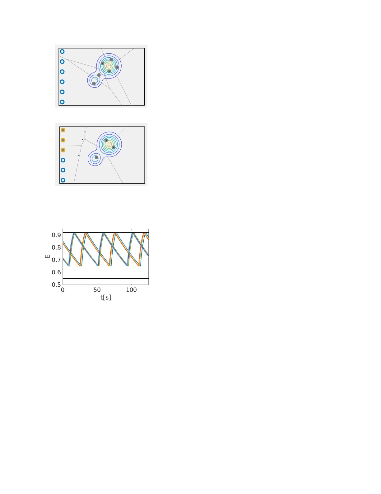
Constrain t Learning for Con trol T asks with Limited Duration Barrier F unctions ? Moto ya Ohnishi a , b , Gennaro Notomista c , Masashi Sugiy ama a , d Magn us Egerstedt e a RIKEN Center for A dvanc e d Intel ligenc e Pr oje ct T okyo 103-0027, Jap an b Paul G. Al len Scho ol of Computer Scienc e and Engine ering, University of Washington Se attle, W A 98195 USA c Scho ol of Me chanic al Engine ering, Ge or gia Institute of T e chnolo gy Atlanta, GA 30313 USA d Dep artment of Complexity Scienc e and Engine ering, University of T okyo Chib a 277-8561, Jap an e Scho ol of Ele ctric al and Computer Engineering, Ge or gia Institute of T e chnolo gy Atlanta, GA 30332 USA Abstract When deplo ying autonomous agen ts in unstructured en vironments o v er sustained perio ds of time, adaptabilit y and robustness often times outw eigh optimality as a primary consideration. In other w ords, safet y and surviv abilit y constrain ts pla y a k ey role and in this pap er, we present a nov el, constraint-learning framew ork for control tasks built on the idea of constraints-driv en con trol. Ho w ev er, since con trol policies that k eep a dynamical agent within state constraints o v er infinite horizons are not alw a ys av ailable, this work instead considers constraints that can b e satisfied ov er some finite time horizon T > 0, which w e refer to as limited-duration safet y . Consequently , v alue function learning can b e used as a tool to help us find limited-duration safe policies. W e sho w that, in some applications, the existence of limited-duration safe policies is actually sufficient for long- duration autonomy . This idea is illustrated on a swarm of simulated rob ots that are task ed with co vering a given area, but that sporadically need to abandon this task to c harge batteries. W e sho w how the battery-charging b eha vior naturally emerges as a result of the constrain ts. Additionally , using a cart-pole sim ulation environmen t, we show how a con trol policy can b e efficien tly transferred from the source task, balancing the pole, to the target task, moving the cart to one direction without letting the p ole fall do wn. Key wor ds: Constrain ts, In v ariance, Learning control, Mo del-based control, Kno wledge transfer 1 In tro duction Acquiring an optimal p olicy that attains the maxim um return ov er some time horizon is of primary in terest in the literature of b oth reinforcement learning [27] and optimal con trol [13]. A large num b er of algorithms ha ve b een designed to successfully control systems with com- ? Corresp onding author M. Ohnishi. (Paul G. Allen Sc ho ol of CS & E) T el. +1 206-543-1695. F ax +1 206-543-2969. Email addr esses: mohnishi@cs.washington.edu (Moto ya Ohnishi), g.notomista@gatech.edu (Gennaro Notomista), sugi@k.u-tokyo.ac.jp (Masashi Sugiyama), magnus@gatech.edu (Magn us Egerstedt). plex dynamics to accomplish sp ecific tasks optimally in some sense. As w e can observe in the daily life, on the other hand, it is often difficult to attribute optimality to h uman b eha viors (cf. [25]). Instead, humans are capable of generalizing the b eha viors acquired through complet- ing a certain task to deal with unseen situations. This fact casts a question of how one should design a learning algorithm that generalizes across tasks. In this pap er, we hypothesize that this can b e achiev ed b y letting agents acquire a set of go o d enough p olicies when completing one task, and reuse this set for an- other task. Sp ecifically , we consider safety , which refers to av oiding certain states, as useful information shared Preprin t submitted to Automatica 8 April 2021 Fig. 1. An illustration of limited-duration safet y . An agent sta ys in O for all 0 ≤ t < T whenev er starting from inside the set C T LD ⊂ O . among different tasks, and we regard limited-duration safe p olicies as goo d enough p olicies (Definition 3). Our w ork is built on the idea of constrain ts-driven control [5,15], a methodology for controlling agents through en- forcemen t of state constraints. Ho w ever, state constraints cannot b e alw a ys satisfied o v er an infinite-time horizon. W e tac kle this feasibility issue b y relaxing safet y to limite d-dur ation safety , by whic h we mean satisfaction of safety o ver some finite time horizon T > 0 (see Figure 1). T o guarantee limited- duration safety , we prop ose a limited duration control barrier function (LDCBF). The idea is based on local, mo del-based control that constrains the instantaneous con trol input every time to restrict the gro wths of v alues of LDCBFs by solving a quadratic programming (QP). T o find an LDCBF, w e mak e use of v alue function learn- ing, and show that the v alue function associated with an y giv en p olicy b ecomes an LDCBF (Section 4.2). Con- trary to the optimal con trol approaches that only single out an optimal policy , our framework can b e contextual- ized within the so-called lifelong learning [31] and trans- fer learning [20]; see Section 5.2). The rest of this pap er is organized as follo ws: Section 2 discusses the related w ork, Section 3 presents notations, assumptions made in this pap er, and some background kno wledge. Subsequently , w e present our main contribu- tions and their applications, including simulated exp er- imen ts, in Section 4 and 5, resp ectively . 2 Related W ork Finding feasible con trol constraints that translate to state constraints has b een of particular interest b oth in the controls and machine learning communities. Early w ork includes the construction of na vigation functions in terms of obstacle a voidance [24]. Alternatively , existence of a control Ly apunov function (CLF) [26] enables stabi- lization of the system, and CLFs may b e learned through demonstrations [10]. As inv erse optimality [6] dictates that a stabilizing p olicy is equiv alent to an optimal p ol- icy in terms of some cost function, these approaches ma y b e viewed as optimization-based techniques. On the other hand, control barrier functions (CBFs) [36,34,1,7,18,19] were prop osed to guaran tee forw ard in- v ariance [9] of a certain region of the state space. The idea of constraints-driv en con trols is in stark contrast to finding one optimal tra jectory to some specific task. Ho w ever, although there exist conv erse theorems whic h claim that a forward inv arian t set has a barrier func- tion under certain conditions [23,35,1], finding such a set without assuming stabilit y of the system (e.g. [33]) is difficult in general. Besides, transfer learning is a framework for learning new tasks b y exploiting the knowledge already acquired through learning other tasks, and is related to ”lifelong learning” [31]. Our w ork can be used as a transfer learn- ing tec hnique b y regarding a set of go od enough policies as useful information shared among other tasks. In the next section, we presen t some assumptions to- gether with the notations used in the pap er. 3 Preliminaries Throughout, R , R ≥ 0 and Z + are the sets of real num b ers, nonnegativ e real num b ers and p ositiv e integers, resp ec- tiv ely . Let k·k R d := p h x, x i R d b e the norm induced b y the inner pro duct h x, y i R d := x T y for d -dimensional real v ectors x, y ∈ R d , where ( · ) T stands for transp osition. Also, let C 1 ( A ) b e a class of contin uously differentiable function defined ov er A . The interior and the b oundary of a set A are denoted b y int( A ) and ∂ A , resp ectively . In this pap er, we consider an agent with system dynamics describ ed by an ordinary differential equation: dx dt = f ( x ( t )) + g ( x ( t )) u ( t ) , (1) where x ( t ) ∈ R n x and u ( t ) ∈ U ⊂ R n u are the state and the instantaneous control input of dimensions n x , n u ∈ Z + , f : R n x → R n x , and g : R n x → R n x × n u . Let D b e the state space whic h is an op en connected subset of R n x , and let X ⊂ D be its compact subset. The Lie deriv ativ es along f and g are denoted by L f and L g . In this work, we make the following assumptions. Assumption 1. F or any lo c al ly Lipschitz c ontinuous p olicy φ : D → U , f + g φ is lo c al ly Lipschitz over D . Assumption 2. The c ontr ol sp ac e U ( ⊂ R n u ) is a p oly- he dr on. With these preliminaries in place, w e presen t the main con tribution. 4 Constrain t Learning for Con trol T asks In this section, we prop ose limite d dur ation c ontr ol b ar- rier functions (LDCBFs), and present their prop erties and a practical wa y to find an LDCBF. 2 4.1 Limite d Dur ation Contr ol Barrier F unctions W e start this section by the following definition. Definition 1 (Limited-duration safet y) . Given an op en set of safe states O ⊂ D , let C T LD b e a close d nonempty subset of O . The dynamic al system (1) is said to b e safe up to time T , if ther e exists a p olicy φ that ensur es x ( t ) ∈ O for al l 0 ≤ t < T whenever x (0) ∈ C T LD . Giv en B LD : D → R ≥ 0 of class C 1 ( D ), let O :=  x ∈ X : B LD ( x ) < L β  , L > 0 , β > 0 , (2) C T LD =  x ∈ X : B LD ( x ) ≤ Le − β T β  ⊂ O , (3) for some T > 0. Now, LDCBFs are defined by b elo w. Definition 2 (Limited duration con trol barrier func- tion) . A function B LD : D → R ≥ 0 of class C 1 ( D ) is c al le d a limite d dur ation c ontr ol b arrier function (LD- CBF) for O define d by (2) and for T if the fol lowing c onditions ar e met: (1) O ⊂ in t( X ) . (2) C T LD define d by (3) is nonempty and ther e exists a monotonic al ly incr e asing lo c al ly Lipschitz c ontinu- ous function 1 α : R → R such that α (0) = 0 and inf u ∈U { L f B LD ( x ) + L g B LD ( x ) u } ≤ α  Le − β T β − B LD ( x )  + β B LD ( x ) , ∀ x ∈ O . Giv en an LDCBF, the admissible control space S T LD ( x ) , x ∈ O , is defined by S T LD ( x ) := { u ∈ U : L f B LD ( x ) + L g B LD ( x ) u ≤ α  Le − β T β − B LD ( x )  + β B LD ( x ) } . (4) If the initial state is taken in C T LD and an admissible con trol is employ ed, safety up to time T is guaranteed. Theorem 1. Supp ose that a set of safe states O define d by (2) and an LDCBF B LD define d on D ar e given. Sup- p ose also that x (0) ∈ C T LD , wher e C T LD is define d by (3). Then, under Assumption 1, any lo c al ly Lipschitz c ontinu- ous p olicy φ : D → U that satisfies φ ( x ) ∈ S T LD ( x ) , ∀ x ∈ O , r enders the dynamic al system (1) safe up to time T . Pr o of. See App endix A. In practice, one can constrain the con trol input within the admissible control space S T LD ( x ) , x ∈ O , via QPs in the same manner as CBFs and CLFs. 1 Note α is not necessarily an extended class- K function [9]. Prop osition 1. Given an LDCBF B LD with a lo c al ly Lipschitz derivative and the admissible c ontr ol sp ac e S T LD ( x ∗ ) at x ∗ ∈ O define d by (4), c onsider the QP: φ ( x ∗ ) = argmin u ∈S T LD ( x ) u T H ( x ∗ ) u + 2 b ( x ∗ ) T u, wher e H and b ar e Lipschitz c ontinuous at x ∗ ∈ O , and H ( x ∗ ) = H T ( x ∗ ) is p ositive defin ite. If the width 2 of a fe asible set is strictly lar ger than zer o, then under As- sumption 2, the minimizers φ ( x ∗ ) ar e unique and Lips- chitz with r esp e ct to the state at x ∗ . Pr o of. Slight mo difications of [16, Theorem 1] prov es the prop osition. Remark 1. Assumption 2 is r e quir e d for the c onstr aints to b e entir ely expr esse d as the interse ction of finite affine c onstr aints. As such, through LDCBFs, global prop ert y (i.e., limited- duration safet y) is ensured b y constraining instanta- neous control inputs. A b enefit of considering LDCBFs is that one can systematically obtain it under mild con- ditions. 4.2 Finding a Limite d Dur ation Contr ol Barrier F unc- tion W e presen t a possible w ay to find an LDCBF B LD for the set of safe states through v alue function learning. Here, w e should men tion that, in practice, one ma y consider cases where a nominal mo del or a simulator is av ailable to learn LDCBF during training time, or cases where getting outside of safe regions during training is not ”fa- tal” (e.g., breaking the agen t). Let ` : D → R ≥ 0 , b e the immediate cost 3 , and supp ose O ⊂ in t( X ) where the set of safe states O is given by O := { x ∈ D : ` ( x ) < L } , L > 0 . Giv en a policy φ : D → U , supp ose that the system (1) is lo cally Lipsc hitz and that the initial condition x (0) = x is in O . Then, following the first argument in App endix A, x ( t ) can b e uniquely defined b y extending the solution un til reac hing ∂ X . Let T e ( x ) b e the first time at which the tra jectory x ( t ) exits O when x (0) = x ∈ O . No w, we define the v alue function V φ,β : D → R ≥ 0 b y V φ,β ( x ) := ( R T e ( x ) 0 e − β t ` ( x ( t )) dt + Le − β T e ( x ) β ( x ∈ O ) ` ( x ) β ( x ∈ D \ O ) 2 See App endix B for the definition. 3 In this paper, we consider the costs that do not dep end on control inputs. 3 where β > 0 is the discoun t factor. When the restriction of V φ,β to O , denoted by V φ,β | O , is of class C 1 ( O ), we obtain the contin uous-time Bellman equation [12]: β V φ,β ( x ) = L f V φ,β ( x ) + L g V φ,β ( x ) φ ( x ) + ` ( x ) , ∀ x ∈ O . (5) No w, for V φ, 0 ( x ) := R ∞ 0 ` ( x ( t )) dt, x ∈ O , to exist and to b e a CLF that ensures controlled inv ariance of its sublev el sets, one m ust at least assume that the policy φ stabilizes the agent in a state x ∗ ∈ O where ` ( x ∗ ) = 0 and ` ( x ) > 0 , ∀ x ∈ O \ { x ∗ } , whic h is restrictive. Instead, one can use V φ,β as an LDCBF when β > 0. Let ˆ V φ,β : D → R ≥ 0 of class C 1 ( D ) denote an approxi- mation of V φ,β . Since V φ,β ( x ) ≥ L β for all x ∈ D \ O by definition, it follows that  x ∈ D : V φ,β ( x ) < L β  ⊂ O ⊂ int( X ) . Therefore, w e wish to use the approximation ˆ V φ,β as an LDCBF for the set O ; ho wev er, b ecause it has an appro x- imation error, w e take the following steps to guaran tee limited-duration safet y . Using (5), define the estimated immediate cost function ˆ ` b y ˆ ` ( x ) = β ˆ V φ,β ( x ) − L f ˆ V φ,β ( x ) − L g ˆ V φ,β ( x ) φ ( x ) , ∀ x ∈ O . Select c ≥ 0 so that ˆ ` c ( x ) := ˆ ` ( x ) + c ≥ 0 for all x ∈ O , and define the function ˆ V φ,β c ( x ) := ˆ V φ,β ( x ) + c β . Theorem 2. Given T > 0 , c onsider the set ˆ C T LD = ( x ∈ X : ˆ V φ,β c ( x ) ≤ ˆ Le − β T β ) , (6) wher e ˆ L := inf y ∈ X \ O β ˆ V φ,β c ( y ) . If ˆ C T LD is nonempty, then ˆ V φ,β c ( x ) is an LDCBF for T and for the set ˆ O := ( x ∈ X : ˆ V φ,β c ( x ) < ˆ L β ) ⊂ O . Pr o of. See App endix C. Remark 2. The pr o c e dur es ab ove b asic al ly c onsiders mor e c onservative sets ˆ C T LD and ˆ O so that the appr oxima- tion err or incurr e d by using ˆ V φ,β c is taken into ac c ount. One c an sele ct sufficiently lar ge c and sufficiently smal l ˆ L in pr actic e to make the set of safe states mor e c onser- vative. T o enlar ge the set C T LD , the imme diate c ost ` ( x ) is pr eferr e d to b e close to zer o for x ∈ O , and L ne e ds to b e sufficiently lar ge. Also, to make T as lar ge as p os- sible, the given p olicy φ should ke ep the system safe up to sufficiently long time (se e also Definition 3 for go o d enough policy ); given a p olicy, the lar ger T one sele cts the smal ler the set C T LD b e c omes. In addition, when ` ( x ) is almost zer o inside O and when L  1 , the choic e of β do es not matter signific antly to c onservativeness of C T LD . As our approac h is set-theoretic rather than sp ecifying a single optimal p olicy , it is also compatible with the constrain ts-driv en control and transfer learning. 5 Applications In this section, w e present tw o practical applications of LDCBFs, namely , long-duration autonomy and transfer learning. 5.1 Applic ations to L ong-dur ation Autonomy In many applications, guaran teeing particular prop erties (e.g., forward in v ariance) ov er an infinite-time horizon is difficult. Nevertheless, it is often sufficient to guaran- tee safety up to certain finite time, and our prop osed LDCBFs act as useful relaxations of CBFs. T o see that one can still achiev e long-duration autonomy b y using LDCBFs, we consider the settings of work in [17]. 5.1.1 Pr oblem F ormulation Supp ose that the state x := [ E , p T ] T ∈ R 3 has the infor- mation of energy level E ∈ R ≥ 0 and the position p ∈ R 2 of an agent, and the dynamics is given by (1) for f ( x ) = [ ˆ F ( x ) , F ( x )] T , g ( x ) = [ ˆ G ( x ) , G ( x )] T , where ˆ F : R 3 → R , F : R 3 → R 2 , ˆ G : R 3 → R 2 , and G : R 3 → R 2 × 2 . Supp ose also that the minimum necessary energy level E min and the maximum energy lev el E max satisfy 0 < E min < E max , and that ρ ( p ) ≥ 0 (equalit y holds only when the agent is at a charging station) is the energy required to bring the agent to a c harging station from p ∈ R 2 , where ρ ∈ C 1 ( R 2 ). Define ∆ E := E max − E min and X := { x ∈ R 3 : E min ≤ E ≤ E max ∧ 0 ≤ ρ ( p ) ≤ ∆ E } . Also, let U ⊂ R 2 b e a control space. The open connected set D ⊃ X is assumed to b e prop erly chosen. Then, for L := β · ∆ E , β > 0, we define B LD : D → R ≥ 0 b y B LD ( x ) := ˜ H  ( E ) + ρ ( p ) , where ∆ E 4   > 0 and ˜ H  ( E ) = E max − E for ∀ E < E max − 3  (see App endix D for the detailed definition, whic h ensures O ⊂ in t( X )). Given T > 0, we can define O and C T LD b y (2) and (3). Note x ∈ O implies E > E min + ρ ( p ). 4 Assumption 3. The ener gy dynamics satisfies ∃ K d > 0 , dE dt = ˆ F ( x ) + ˆ G ( x ) u ≥ − K d , ∀ x ∈ D , ∀ u ∈ U , and is upp er b ounde d by dE dt ≤ 0 , ∀ x ∈ A ρ ( p )=0 , ∀ u ∈ U , wher e A ρ ( p )=0 := { x ∈ O : ρ ( p ) = 0 } . In addition, the set ˜ S T LD ( x ) := { u ∈ U : L ˜ f B LD ( x ) + L ˜ g B LD ( x ) u ≤ α  Le − β T β − B LD ( x )  + β B LD ( x ) } , (7) is nonempty for al l x ∈ O \ ( A ρ ( p )=0 ∪ A E ) , wher e ˜ f ( x ) = [ − K d , F ( x )] T , ˜ g = [ 0 , G ( x )] T , and A E := { x ∈ O : E ≥ E max − 4  } . Remark 3. Supp ose S T LD ( x ) is nonempty for al l x ∈ A ρ ( p )=0 ∪A E . Supp ose also that Assumption 3 holds, then B LD is an LDCBF for O and T s.t. C T LD is nonempty, b e c ause ˜ S T LD ( x ) ⊂ S T LD ( x ) for al l x ∈ O \ ( A ρ ( p )=0 ∪ A E ) . Assumption 3 implies that the least p ossible exit time ˆ T energy ( E ) of E > E min b eing b elow E min is ˆ T energy ( E ) = ( E − E min ) K d . Under these settings, the follo wing prop osition holds. Prop osition 2. Supp ose Assumption 1 and Assumption 3 hold, and that T > ˆ T energy ( E 0 ) for the initial ener gy level E max − 4  ≥ E 0 > E min . Supp ose also that x (0) ∈ C T LD , and that a lo c al ly Lipschitz c ontinuous p olicy φ : D → U satisfies φ ( x ) ∈ ˜ S T LD ( x ) for al l x ∈ O \ ( A ρ ( p )=0 ∪ A E ) . F urther, assume the maximum interval of existenc e of unique solutions E t and ρ t , namely, the tr aje ctories of E and ρ ( p ) , is given by [0 , T ∗ ) for some T ∗ > 0 . Then, T ρ t =0 := inf { t ∈ [0 , T ∗ ) : ρ t = 0 } ≤ T energy := inf { t ∈ [0 , T ∗ ) : E t − E min ≤ 0 } . Pr o of. See App endix E. Remark 4. When a function B LD satisfying Assump- tion 3 and the set O ar e given, we assume that ˜ S T LD define d for a smal ler c onstant β ∗ < β , inste ad of β , is nonempty as wel l. Then the agent stays in O longer than T if taking the c ontr ol input in ˜ S T LD starting fr om inside C T LD , which is define d for β . In this c ase, ther e is a tr ade-off b etwe en β and T . Remark 5. Inste ad of assuming (7), one may le arn an LDCBF fol lowing the ar guments in Se ction 4.2. In such a c ase, the imme diate c ost function ` ( x ) may b e de- fine d so that 0 ≤ ` ( x )  1 for E ∈ ( E min , E max ) and that ` ( x ) ≥ 1 otherwise. Then, one may le arn the value function of some p olicy for the system wher e ˆ F ( x ) = − K d , ∀ x ∈ O \ A ρ ( p )=0 , ˆ G ( x ) = 0 , ∀ x ∈ O , and ∃ y ∈ A ρ ( p )=0 , ∃ K i > 0 , ˆ F ( y ) ≥ K i . If ˆ C T LD define d by (6) is nonempty for T > ˆ T energy ( E 0 ) , then similar claims to Pr op osition 2 hold. Note the p olicy do es not have to stabilize the system ar ound A ρ ( p )=0 but c an b e anything as long as ˆ C T LD b e c omes nonempty. 5.1.2 Simulate d Exp eriment Let the parameters be E max = 1 . 0, E min = 0 . 55, K d = 0 . 01, β = 0 . 005 and T = 50 . 0 > 45 . 0 = ∆ E /K d . W e consider six agents (rob ots) with single integrator dynamics. An agent of the p osition p i := [x i , y i ] T is assigned a charging station of the position p charge ,i , where x and y are the X p osition and the Y p osition, resp ectiv ely . When the agent is close to the station (i.e., k p i − p charge ,i k R 2 ≤ 0 . 05), it remains there un til the battery is char ged to E ch = 0 . 92. Actual battery dynamics is giv en by dE /dt = − 0 . 01 E . The co verage con trol task is encoded as Llo yd’s algorithm [3] aiming at con verging to the Cen troidal V oronoi T esselation, but with a soft margin so that the agen t prioritizes the safety constraint. The lo cational cost used for the co v erage control task is given by the following [4]: 6 X i =1 Z V i ( p ) k p i − ˆ p k 2 ϕ ( ˆ p ) d ˆ p, where V i ( p ) = { ˆ p ∈ R 2 : k p i − ˆ p k ≤ k p j − ˆ p k , ∀ j 6 = i } is the V oronoi cell for the agen t i . In particular, w e used ϕ ([ˆ x , ˆ y] T ) = e − { (ˆ x − 0 . 2) 2 +(ˆ y − 0 . 3) 2 } / 0 . 06 + 0 . 5 e − { (ˆ x+0 . 2) 2 +(ˆ y+0 . 1) 2 } / 0 . 03 . In MA TLAB simulation (the simulator is provided on the Rob otarium [22] web- site: www.rob otarium.org), w e used the random seed rng(5) for determining the initial states. Note, for every agen t, the energy level and the position are set so that it starts from inside the set C T LD . Note also that battery information is lo cal to each agent who has its own LD- CBFs 4 ; limited-duration safet y is th us enforced in a decen tralized manner. Figure 2 shows (a) the images of six agents executing co v erage tasks and (b) images of the agents three of whic h are charging their batteries. Figure 3 shows the sim ulated battery voltage data of the six agen ts, from whic h w e can observe that LDCBFs w orked effectively 4 W e are implicitly assuming that B LD is an LDCBF, i.e., the conditions in Remark 3 are satisfied. 5 (a) (b) Fig. 2. (a) Screenshot of agents executing co verage controls. (b) Screenshot of agents three of which are charging their batteries. Fig. 3. Battery levels of the six agents ov er time. Tw o blac k lines indicate the energy level when charged ( E ch = 0 . 92) and the minimum energy level ( E min = 0 . 55). All agents successfully executed tasks without depleting their batteries. for the swarm of agents to av oid depleting their batteries. 5.2 Applic ations to T r ansfer L e arning Another b enefit of using LDCBFs is that, once a set of go o d enough p olicies that guaran tee limited-duration safet y for sufficiently large T and for sufficiently large C T LD is obtained, one can reuse them for different tasks. Definition 3 (Go od enough p olicy) . Supp ose a p olicy φ guar ante es safety up to time T if the initial state is in C T LD ⊂ D . Supp ose also that an initial state of a task T is always taken in C T LD and that the task c an b e achieve d within the time horizon T . Then, the p olicy φ is said to b e go od enough with r esp e ct to the task T . W e introduce the definition of transfer learning b elow. Definition 4 (T ransfer learning, [20, mo dified version of Definition 1]) . Given a set of tr aining data D S for one task (i.e., sour c e task) denote d by T S (e.g., an MDP) and a set of tr aining data D T for another task (i.e., tar get task) denote d by T T , tr ansfer le arning aims to impr ove the le arning of the tar get pr e dictive function f T (i.e., a p olicy in our example) in D T using the know le dge in D S and T S , wher e D S 6 = D T , or T S 6 = T T . In our example, w e assume we know the state constraints that a target task T T is b etter to satisfy and that some of these constrain ts are shared with a source task T S . If a set of training data D S is used to obtain a go o d enough p olicy for the source task, one can learn an LDCBF with this policy . When this p olicy is also go od enough for the target task, whic h would be the case if some constrain ts are shared with a target task, then the learned LDCBF is exp ected to b e used to sp eed up the learning of the target task. 5 5.2.1 Il lustr ative Example F or example, when learning a go o d enough p olicy for the balance task of the cart-p ole problem, one can si- m ultaneously learn a set of limited-duration safe policies that keep the p ole from falling down up to certain time T > 0. The set of these limited-duration safe p olicies is ob viously useful for other tasks such as moving the cart to one direction without letting the p ole fall down. W e study some practical implementations. Given an LD- CBF B LD , define the set Φ T of admissible p olicies as Φ T := { φ ⊂ Φ : φ ( x ) ∈ S T LD ( x ) , ∀ x ∈ O } , where Φ := { φ : φ ( x ) ∈ U , ∀ x ∈ D } , and S T LD ( x ) is the set of admissible control inputs at x . If an optimal p olicy φ T T for the target task T T is included in Φ T , one can conduct learning for the target task within the p olicy space Φ T . If not, one can still consider Φ T as a soft constrain t and explore the p olicy space Φ \ Φ T with a giv en probability or one may just select the initial p olicy from Φ T . In practice, a parametrized policy is usually considered; a p olicy φ θ expressed by a parameter θ ∈ R n θ for n θ ∈ Z + is up dated via policy gradient methods [28]. If the p olicy is in the linear form with a fixed feature vector, the pro jected p olicy gradient metho d [30] can be used. Giv en, a set of finite data p oin ts D ⊂ X , the p olicy φ ( x ) is linear with respect to θ at eac h x ∈ D and that LDCBF constrain ts are affine with resp ect to φ ( x ) at eac h x ∈ D ; therefore, ˜ Φ T θ := { θ ∈ R n θ : φ θ ( x ) ∈ S T LD ( x ) , ∀ x ∈ 5 F urther study of rigorous sample complexit y analysis for this transfer learning framew ork is b ey ond the scope of this pap er. 6 D } is an in tersection of finite affine constrain ts, whic h is a p olyhedron. Hence, the pro jected p olicy gradient metho d lo oks like θ ← Γ[ θ + λ ∇ θ F T T ( θ )]. Here, Γ : R n θ → ˜ Φ T θ pro jects a p olicy onto ˜ Φ T θ and F T T ( θ ) is the ob jective function for the target task which is to b e maximized. F or the p olicy not in the linear form, one ma y up date p olicies based on LDCBFs by mo difying the deep deterministic p olicy gradien t (DDPG) metho d [14]: because through LDCBFs, the global prop erty (i.e., limited-duration safet y) is ensured b y constraining lo cal con trol inputs, it suffices to add p enalt y terms to the cost when up dating a policy using samples. F or example, one ma y employ the log-barrier extension prop osed in [8], whic h is a smooth approximation of the hard indicator function for inequalit y constrain ts but is not restricted to feasible p oints. 5.2.2 Simulate d Exp eriment The sim ulation en vironment and the deep learning framew ork used in this sim ulated experiment are ”Cart- p ole” in DeepMind Con trol Suite and PyT orch [21], resp ectiv ely . W e take the following steps: (1) Learn a policy that balances the pole by using DDPG [14] ov er sufficiently long time horizon. (2) Learn an LDCBF by using the obtained actor net- w ork. (3) T ry a random p olicy with the learned LDCBF and using a (lo cally) accurate model to see that LDCBF w orks reasonably . (4) With and without the learned LDCBF, learn a p ol- icy that mo v es the cart to left without letting the p ole fall down, which we refer to as mov e-the-p ole task. The parameters use d for this simulated exp erimen t are summarized in T able 1. Here, angle threshold stands for the threshold of cos ψ where ψ is the angle of the p ole from the standing position, and position threshold is the threshold of the cart position p . The angle threshold and the position threshold are used to terminate an episo de. Note that the cart-p ole en vironment of MuJoCo [32] xml data in DeepMind Control Suite is mo dified so that the cart can mo ve betw een − 3 . 8 and 3 . 8. W e use prioritized exp erience repla y when learning an LDCBF. Sp ecifically , w e store the p ositiv e and the negative data, and sample 4 data p oin ts from the p ositiv e one and the remaining 60 data p oin ts from the negative one. In this sim ulated ex- p erimen t, actor, critic and LDCBF netw orks use ReLU nonlinearities. The actor netw ork and the LDCBF net- w ork consist of tw o la yers of 300 → 200 units, and the critic netw ork is of t wo lay ers of 400 → 300 units. The con trol input v ector is concatenated to the state vector from the second critic la y er. Step1: The av erage duration (i.e., the first exit time, namely , the time when the p ole first falls down) out of 10 seconds (corresponding to 1000 time steps), o ver 10 trials for the p olicy learned through the balance task b y DDPG was 10 seconds. Step2: Then, b y using this successfully learned p olicy , an LDCBF is learned by assigning the cost ` ( x ) = 1 . 0 for cos ψ < 0 . 2 and ` ( x ) = 0 . 1 elsewhere. Also, b ecause the LDCBF is learned in a discrete-time form, we trans- form it to a contin uous-time form via multiplying it by ∆ t = 0 . 01. When learning an LDCBF, w e initialize each episo de as follows: the angle ψ is uniformly sampled within − 1 . 5 ≤ ψ ≤ 1 . 5, the cart velocity ˙ p is multiplied b y 100 and the angular velocity ˙ ψ is m ultiplied b y 200 after b eing initialized by DeepMind Control Suite. The LDCBF learned by using this p olicy is illustrated in Fig- ure 4, which agrees with our intuitions. Note that L β in this case is 1 . 0 − log (0 . 999) / 0 . 01 ≈ 10 . 0. Step3: T o test this LDCBF, w e use a uniformly random p olicy ( φ ( x ) tak es the v alue b etw een − 1 and 1) constrained by the LDCBF with the func- tion α ( q ) = max { 0 . 1 q , 0 } and with the time constant T = 5 . 0. When imp osing constrain ts, we use the (lo- cally accurate) con trol-affine mo del of the cart-p ole in the work [2], where we replace the friction parameters b y zeros for simplicit y . The av erage duration out of 10 seconds ov er 10 trials for this random p olicy w as 10 seconds, which indicates that the LDCBF work ed suffi- cien tly well. W e also tried this LDCBF with the func- tion α ( q ) = max { 3 . 0 q , 0 } and T = 5 . 0, which resulted in the a v erage duration of 5 . 58 seconds. Moreov er, we tried the fixed policy φ ( x ) = 1 . 0, with the function α ( q ) = max { 0 . 1 q , 0 } and T = 5 . 0, and the av erage du- ration was 4 . 73 seconds, whic h was sufficiently close to T = 5 . 0. Step4: F or the mov e-the-p ole task, we define the suc- cess by the situation where the cart p osition p, − 3 . 8 ≤ p ≤ 3 . 8, ends up in the region of p ≤ − 1 . 8 without letting the p ole fall down. The angle ψ is uniformly sampled within − 0 . 5 ≤ ψ ≤ 0 . 5 and the rest follow the initialization of DeepMind Control Suite. The reward is given by (1 + cos ψ ) / 2 × (utils.rewards.tolerance( ˙ p + 1 . 0, b ounds = ( − 2 . 0 , 0 . 0), margin = 0 . 5)), where utils.rew ards.tolerance is the function defined in [29]. In other words, we give high rewards when the cart v elo cit y is negative and the p ole is standing up. T o use the learned LDCBF for DDPG, w e store matrices and v ectors used in linear constrain ts along with other v ari- ables such as control inputs and states, whic h we use for exp erience replay . Then, the log-barrier extension cost prop osed in [8] is added when up dating p olicies. Also, w e try DDPG without using the LDCBF for the mo v e-the-p ole task. Both approac hes initialize the pol- icy by the one obtained after the balance task. The a v erage success rates of the p olicies obtained after the n um b ers of episo des up to 15 ov er 10 trials are given in T able 2 for DDPG with the learned LDCBF and DDPG 7 1.5 1.0 0.5 0.0 0.5 1.0 angle (sin) 2 1 0 1 2 angular vel (rad/sec) 4.80 5.84 6.88 7.92 8.96 10.00 11.04 12.08 13.12 14.16 Fig. 4. Illustration of the LDCBF for sin ψ and ˙ ψ at zero cart v elo cit y . The cen ter has lo wer v alue. Also, unsafe regions ha v e the v alues ov er L β = 1 . 0 − log (0 . 999) / 0 . 01 ≈ 10 . 0. without LDCBF. This result implies that our prop osed approac h successfully transferred information from the source task to the target task. 6 Conclusion In this pap er, w e presented a notion of limited-duration safet y as a relaxation of forward in v ariance of a set of safe states. Then, w e prop osed limited-duration control barrier functions to guaran tee limited-duration safety b y using agen t dynamics. W e show ed that LDCBFs can b e obtained through v alue function learning, and ana- lyzed some of their prop erties. LDCBFs were v alidated through p ersistent co verage control tasks and were suc- cessfully applied to a transfer learning problem b y shar- ing a common state constrain t. Ac knowledgemen ts M. Ohnishi thanks Kai Koike at Kyoto Universit y for v aluable discussions on differential equations. The au- thors thank the anon ymous reviewers for their careful and constructive commen ts that help ed us improv e this w ork. This work of M. Ohnishi was supp orted in part b y F unai Ov erseas Scholarship and Wissner-Slivk a En- do w ed Graduate F ellowship. This w ork of G. Notomista and M. Egerstedt w as supp orted b y the US Arm y Re- searc h Lab through Gran t No. DCIST CRA W911NF- 17-2-0181. This work of M. Sugiy ama was supp orted b y KAKENHI 17H00757. A Pro of of Theorem 1 Under Assumption 1, the tra jectories x ( t ) with an initial condition x (0) ∈ C T LD ⊂ D exist and are unique ov er 0 ≤ t ≤ δ for some δ > 0. Let [0 , T ∗ ) , T ∗ > 0, b e its maxim um interv al of existence ( T ∗ can be ∞ ), and let T e b e the first time at whic h the tra jectory x ( t ) exits O , i.e., T e := inf { t ∈ [0 , T ∗ ) : x ( t ) / ∈ O } . (A.1) Because B LD ∈ C 1 ( D ) and O ⊂ in t( X ) imply O is op en, it follows that T e > 0. If T ∗ is finite, it must b e the case that x ( t ∗ ) / ∈ X for some t ∗ ∈ [0 , T ∗ ) which implies 0 ≤ t ≤ T X < T ∗ , where T X := inf { t ∈ [0 , T ∗ ) : x ( t ) ∈ ∂ X } . In this case, b ecause O ⊂ int( X ), it follows that 0 < T e ≤ T X < T ∗ . If, on the other hand, T ∗ = ∞ , then T e can still b e defined by (A.1), and either T e = ∞ or T e < T ∗ hold. When T e = ∞ , it is straightforw ard to pro v e the claim; therefore, we focus on the case where T e is finite and T e < T ∗ . Let T p denote the last time at whic h the tra jectory x ( t ) passes through the boundary of C T LD from inside b efore first exiting O , i.e., T p := sup  t ∈ [0 , T e ) : x ( t ) ∈ ∂ C T LD  . Because C T LD is closed subset of the op en set O and b e- cause x (0) ∈ C T LD , b y con tinuit y of the solution, it follows that 0 ≤ T p < T e . Now, the solution to ˙ s ( t ) = β s ( t ) , where the initial condition is given by s ( T p ) = B LD ( x ( T p )) = Le − β T β , is s ( t ) = B LD ( x ( T p )) e β ( t − T p ) , ∀ t ≥ T p . It thus follows that s ( T p + T ) = L β e − β T e β T = L β , and T p + T is the first time at which the tra jectory s ( t ) , t ≥ T p , reaches L β . Because α ( Le − β T β − B LD ( t )) ≤ 0 , ∀ t ∈ [ T p , T e ), and φ ( x ) ∈ S T LD ( x ) , ∀ x ∈ O , we obtain, b y the Compar- ison Lemma [9], [11, Theorem 1.10.2] and b y con tinu- it y of the solutions o ver t ∈ [0 , T e ], that B LD ( x ( t )) ≤ s ( t ) , ∀ t ∈ [ T p , T e ]. If we assume T e < T p + T , it follows that B LD ( x ( T e )) ≤ s ( T e ) < s ( T p + T ) = L β whic h is a con tradiction b ecause O ∈ int( X ) and B LD ∈ C 1 ( D ) im- ply B LD ( x ( T e )) = L β . Hence, T e ≥ T p + T , which pro ves the Theorem. 8 T able 1 Summary of the parameter settings for the cart-p ole problem. These parameters are chosen so that a p olicy for the balance task can b e obtained, an LDCBF can be learned, and the mov e-the-p ole task can b e accomplished within 15 episo des when using an LDCBF. W e could not find parameters that make the mov e-the-pole task work without LDCBFs within 15 episo des. P arameters Balance task F or Learning Mov e-the-p ole task Mo v e-the-pole task an LDCBF with LDCBF without LDCBF Discoun t β − log (0 . 99) / 0 . 01 − log (0 . 999) / 0 . 01 − log (0 . 999) / 0 . 01 − log (0 . 999) / 0 . 01 Angle threshold cos ψ thre 0.75 0.2 0.75 0.75 P osition threshold p thre ± 1.8 ± 3.8 ± 3.8 ± 3.8 Soft-up date µ 10 − 3 10 − 2 10 − 3 10 − 3 Step size for target NNs 10 − 4 10 − 2 10 − 4 10 − 4 Time steps p er episode 300 50 300 300 Num b er of episodes 80 200 Up to 15 Up to 15 Minibatc h size 64 64 64 64 Random seed 10 10 10 10 States x sin ψ , 0 . 1 ˙ p, 0 . 1 ˙ ψ sin ψ , ˙ p, ˙ ψ sin ψ , ˙ p, ˙ ψ sin ψ , ˙ p, ˙ ψ T able 2 Summary of the results for the mov e-the-p ole task. Over 15 episo des, the success rates ov er 10 trials are shown. DDPG with LDCBF uses learned LDCBF to constrain con trol inputs when updating p olicies by DDPG, and DDPG without LDCBF do es not use LDCBFs. By using LDCBFs the mov e-the-p ole task is shown to b e easily learned. Algorithm \ Episo de 1 2 3 4 5 6 7 8 9 10 11 12 13 14 15 DDPG with LDCBF 0.0 0.0 0.0 0.4 0.7 0.8 1.0 1.0 1.0 0.7 0.7 1.0 1.0 1.0 1.0 DDPG without LDCBF 0.0 0.0 0.0 0.0 0.0 0.0 0.0 0.0 0.0 0.0 0.0 0.0 0.0 0.0 0.0 B On Proposition 1 The width of a feasible set is defined b y the unique so- lution to the following linear program: ω ∗ ( x ) = max [ u T ,ω ] T ∈ R n u +1 ω (B.1) s . t . L f B LD ( x ) + L g B LD ( x ) u + ω ≤ α  Le − β T β − B LD ( x )  + β B LD ( x ) u + [ ω , ω . . . , ω ] T ∈ U C Pro of of Theorem 2 Because, by definition, ˆ V φ,β c ( x ) ≥ ˆ L β , ∀ x ∈ X \ O , it follows that ˆ O = ( x ∈ X : ˆ V φ,β c ( x ) < ˆ L β ) ⊂ O . Because ˆ V φ,β c ∈ C 1 ( D ) satisfies L f ˆ V φ,β c ( x ) + L g ˆ V φ,β c ( x ) φ ( x ) = β ˆ V φ,β c ( x ) − ˆ ` c ( x ) , ∀ x ∈ O , and ˆ ` c ( x ) ≥ 0 , ∀ x ∈ O , it follows that L f ˆ V φ,β c ( x ) + L g ˆ V φ,β c ( x ) φ ( x ) ≤ α ˆ Le − β T β − ˆ V φ,β c ( x ) ! + β ˆ V φ,β c ( x ) , for all x ∈ O and for a monotonically increasing lo- cally Lipschitz contin uous function α such that α ( q ) = 0 , ∀ q ≤ 0. Therefore, φ ( x ) ∈ U , ∀ x ∈ O ⊂ in t( X ) and ˆ C T LD 6 = ∅ , where ∅ is the empty set, imply that ˆ V φ,β c is an LDCBF for the set ˆ O and for T . Remark C.1. A sufficiently lar ge c onstant c c ould b e chosen in pr actic e. If ˆ ` c ( x ) > 0 for al l x ∈ O and the value function is le arne d by using a p olicy φ such that φ ( x ) + [ c φ , c φ . . . , c φ ] T ∈ U for some c φ > 0 , then the unique solution to the line ar pr o gr am (B.1) satisfies ω ∗ ( x ) > 0 , ∀ x ∈ O . 9 D Definition of the function ˜ H  F or brevit y , let ¯ E := E max − E and ¯ E 2  := E − E max + 2  . Here, w e giv e the definition of ˜ H  whic h is not practically relev an t but is only required to make O ⊂ in t( X ): ˜ H  ( E ) :=    ¯ E ( ¯ E 2  < −  ) ∆ E 8  2 ( ¯ E 2 2  + 2  ¯ E 2  +  2 ) + ¯ E ( | ¯ E 2  | ≤  ) ∆ E 2  ¯ E 2  + ¯ E (  < ¯ E 2  ) Note ˜ H  ( E ) = ¯ E + ∆ E 4  2 H  ( E 2  ), where H  : R → R is the Hub er function. It is straigh tforw ard to see that E = E max = ⇒ x / ∈ O , which is necessary to make O ⊂ in t( X ). E Pro of of proposition 2 Under Assumption 1, the tra jectories x ( t ) with an ini- tial condition x (0) ∈ C T LD , and hence E t and ρ t , exist and are unique ov er 0 ≤ t ≤ δ for some δ > 0. Let [0 , T ∗ ) b e its maximum interv al of existence ( T ∗ can b e ∞ ), which indeed exists. F ollowing the same argu- men t as in App endix A, w e only fo cus on the case where T e defined by (A.1) is finite and 0 < T e < T ∗ (note T e = ∞ = ⇒ T energy = ∞ and, in this case, the claim is trivially v alidated.) Also, if E t − E min > 0 for all t ∈ [0 , T ∗ ), then T energy = inf ∅ = ∞ , and the claim is trivially v alidated again. Therefore, we assume that T energy < T ∗ . F urther, define ˆ T := inf { t ∈ [0 , T ∗ ) : ρ t = 0 ∧ x ( t ) / ∈ C T LD } , ˆ T e := min n T e , ˆ T o ≤ T energy , T p := sup  t ∈ [0 , T e ) : x ( t ) ∈ ∂ C T LD  . F ollowing the same argumen t as in App endix A, we ha v e 0 ≤ T p < T e . Because it must b e the case that E t > E min , ∀ t ∈ [0 , T p ], we should only consider the case where ρ t > 0 , ∀ t ∈ [0 , T p ]. If w e assume ˆ T e = ˆ T , w e obtain ˆ T ≤ T e ≤ T energy whic h prov es the claim. There- fore, we assume ˆ T e = T e . Let ˆ E t b e the tra jectory follo wing the virtual battery dynamics d ˆ E /dt = − K d with the initial condition ˆ E T p = E T p , and let s ( t ) b e the unique solution to ˙ s ( t ) = β s ( t ) , t ≥ T p , where s ( T p ) = B LD ( x ( T p )) = ∆ E e − β T . Also, let % ( t ) = s ( t ) + ˆ E t − E max , t ≥ T p . Then, the time at whic h s ( t ) reaches ∆ E is T p + T b ecause s ( T + T p ) = B LD ( x ( T p )) e β ( T + T p − T p ) = ∆ E e − β T e β ( T + T p − T p ) = ∆ E . Since we assumed x t / ∈ A ρ ( p )=0 , ∀ t ∈ [0 , T p ], under As- sumption 3, we ha ve ˆ T energy ( E T p ) ≤ ˆ T energy ( E 0 ) < T . F urther, we hav e % ( t ) = B LD ( x ( T p )) e β ( t − T p ) + ˆ E T p − K d ( t − T p ) − E max . Hence, we obtain ˆ T 0 := inf { t ≥ T p : % ( t ) = 0 } ≤ T p + ˆ T energy ( E T p ) . On the other hand, under Assumption 1, the actual bat- tery dynamics can b e written as dE /dt = − K d + ∆( x ), where ∆( x ) ≥ 0. Also, b ecause E 0 ≤ E max − 4  , it follows that E t ≤ E max − 4  for all t ∈ [0 , T ∗ ) under Assumption 3, implying B LD ( x ( t )) = E max − E t + ρ t , ∀ t ∈ [0 , T ∗ ). Therefore, φ ( x ) ∈ ˜ S T LD ( x ) , ∀ x ∈ O \ ( A ρ ( p )=0 ∪ A E ), indicates dB LD ( x ( t )) dt ≤ β B LD ( x ( t )) − ∆( x ( t )) , ∀ t ∈ [ T p , T e ) . Then, b ecause d ( B LD ( x ( t )) − s ( t )) dt ≤ β ( B LD ( x ( t )) − s ( t )) − ∆( x ( t )) ≤ β ( B LD ( x ( t )) − s ( t )) , ∀ t ∈ [ T p , T e ) , and β ( B LD ( x ( T p )) − s ( T p )) = 0, we obtain B LD ( x ( t )) − s ( t ) ≤ − R t 0 ∆( x ( t )) dt, ∀ t ∈ [ T p , T e ). Here, following the same argumen ts as App endix A, we hav e that T e ≥ T p + T > T p + ˆ T energy ( E T p ). F urther, it follows that ρ t − % ( t ) = B LD ( x ( T p )) − s ( t ) + E t − ˆ E t ≤ − Z t 0 ∆( x ( t )) dt + Z t 0 ∆( x ( t )) dt = 0 , ∀ t ∈ [ T p , T e ) , whic h, b y contin uity of the solutions, leads to the in- equalit y ρ t ≤ % ( t ) , ∀ t ∈ [ T p , T e ]. Hence, we conclude that ˆ T ≤ ˆ T 0 ≤ T p + ˆ T energy ( E T p ) < T e . This is a con tradiction to the assumption ˆ T e = T e , from whic h the prop osition is prov ed. References [1] A. D. Ames, X. Xu, J. W. Grizzle, and P . T abuada. Control barrier function based quadratic programs for safety critical systems. IEEE T r ans. Automatic Contr ol , 62(8):3861–3876, 2017. [2] A. G. Barto, R. S. Sutton, and C. W. Anderson. Neuronlike adaptive elements that can solve difficult learning control problems. IEEE T r ans. Systems, Man, and Cyb ernetics , (5):834–846, 1983. 10 [3] J. Cort´ es and M. Egerstedt. Co ordinated control of multi-robot systems: A surv ey . SICE Journal of Contr ol, Me asur ement, and System Integr ation , 10(6):495–503, 2017. [4] J. Cortes, S. Martinez, T. Karatas, and F. Bullo. Coverage control for mobile sensing net works. IEEE T r ans. r obotics and Automation , 20(2):243–255, 2004. [5] M. Egerstedt, J. N. Pauli, G. Notomista, and S. Hutc hinson. Robot ecology: Constrain t-based control design for long duration autonomy . Elsevier Annual R eviews in Contr ol , 46:1–7, 2018. [6] R. A. F reeman and P . V. Kokoto vic. Inv erse optimality in robust stabilization. SIAM Journal on Contr ol and Optimization , 34(4):1365–1391, 1996. [7] P . Glotfelter, J. Cort´ es, and M. Egerstedt. Nonsmooth barrier functions with applications to multi-robot systems. IEEE Contr ol Systems L etters , 1(2):310–315, 2017. [8] H. Kerv adec, J. Dolz, J. Y uan, C. Desrosiers, E. Granger, and I. B. Ayed. Log-barrier constrained CNNs. arXiv pr eprint arXiv:1904.04205 , 2019. [9] H. K. Khalil. Nonlinear systems. Pr entic e-Hal l , 3, 2002. [10] S. M. Khansari-Zadeh and A. Billard. Learning control Lyapuno v function to ensure stability of dynamical system- based robot reac hing motions. R ob otics and Autonomous Systems , 62(6):752–765, 2014. [11] V. Lakshmik antham and S. Leela. Differ ential and Integr al Ine qualities: The ory and Applic ations: V olume I: Or dinary Differ ential Equations . Academic press, 1969. [12] F. L. Lewis and D. V rabie. Reinforcement learning and adaptive dynamic programming for feedback control. IEEE Cir cuits and Systems Magazine , 9(3):32–50, 2009. [13] D. Lib erzon. Calculus of variations and optimal c ontrol the ory: a c oncise intr o duction . Princeton University Press, 2011. [14] T. P . Lillicrap, J. Hunt, Jonathan, A. Pritzel, N. Heess, T. Erez, Y. T assa, D. Silver, and D. Wierstra. Contin uous control with deep reinforcement learning. arXiv pr eprint arXiv:1509.02971 , 2015. [15] T. Lozano-P´ erez and L. P . Kaelbling. A constrain t- based metho d for solving sequen tial manipulation planning problems. In IEEE Pro c. IR OS , pages 3684–3691, 2014. [16] B. Morris, M. J. P ow ell, and A. D. Am es. Sufficien t conditions for the Lipschitz con tinuit y of QP-based multi-ob jectiv e control of h umanoid rob ots. In Pr o c. CDC , pages 2920–2926, 2013. [17] G. Notomista, S. F. Ruf, and M. Egerstedt. Persistification of robotic tasks using control barrier functions. IEEE R ob otics and Automation L etters , 3(2):758–763, 2018. [18] M. Ohnishi, L. W ang, G. Notomista, and M. Egerstedt. Barrier-certified adaptive reinforcement learning with applications to brushbot navigation. IEEE T r ans. Rob otics , 35(5):1186–1205, 2019. [19] M. Ohnishi, M. Y uk aw a, M. Johansson, and M. Sugiyama. Contin uous-time v alue function approximation in repro ducing kernel Hilbert spaces. Pr o c. NeurIPS , pages 2813–2824, 2018. [20] S. J. Pan, Q. Y ang, et al. A survey on transfer learning. IEEE T r ans. Know le dge and Data Engine ering , 22(10):1345–1359, 2010. [21] A. P aszke, S. Gross, S. Chintala, G. Chanan, E. Y ang, Z. DeVito, Z. Lin, A. Desmaison, L. An tiga, and A. Lerer. Automatic differentiation in PyT orch. 2017. [22] D. Pickem, P . Glotfelter, L. W ang, M. Mote, A. Ames, E. F eron, and M. Egerstedt. The Robotarium: A remotely accessible sw arm robotics research testb ed. In IEEE Pr o c. ICRA , pages 1699–1706, 2017. [23] S. Ratschan. Con verse theorems for safet y and barrier certificates. IEEE T r ans. Automatic Contr ol , 63(8):2628– 2632, 2018. [24] E. Rimon and D. E. Ko ditsc hek. Exact robot navigation using artificial potential functions. IEEE T r ans. R ob otics and Automation , 8(5):501–518, 1992. [25] B. F. Skinner. Scienc e and human b ehavior . Num b er 92904. Simon and Sch uster, 1953. [26] E. D. Sontag. A ”universal” construction of Artstein’s theorem on nonlinear stabilization. Systems & c ontr ol letters , 13(2):117–123, 1989. [27] R. S. Sutton and A. G. Barto. Reinfor c ement le arning: An intr o duction . MIT Press, 1998. [28] R. S. Sutton, D. A. McAllester, S. P . Singh, and Y. Mansour. Policy gradien t metho ds for reinforcemen t learning with function appro ximation. In Pr o c. NeurIPS , pages 1057–1063, 2000. [29] Y. T assa, Y. Doron, A. Muldal, T. Erez, Y. Li, D. de L. Casas, D. Budden, A. Abdolmaleki, J. Merel, A. Lefrancq, T. L. Lillicrap, and M. Riedmiller. DeepMind Control Suite. arXiv pr eprint arXiv:1801.00690 , 2018. [30] P . S. Thomas, W. C. Dabney , S. Giguere, and S. Mahadev an. Pro jected natural actor-critic. In Pr o c. NeurIPS , pages 2337– 2345, 2013. [31] S. Thrun and T. M. Mitc hell. Lifelong robot learning. In The Biolo gy and T e chnolo gy of Intel ligent Autonomous A gents , pages 165–196. Springer, 1995. [32] E. T o doro v, T. Erez, and Y. T assa. Mujo co: A physics engine for model-based con trol. In IEEE/RSJ International Confer enc e on Intel ligent R ob ots and Systems , pages 5026– 5033, 2012. [33] L. W ang, D. Han, and M. Egerstedt. Permissiv e barrier certificates for safe stabilization using sum-of-squares. Pr o c. ACC , pages 585–590. [34] P . Wieland and F. Allg¨ ower. Constructiv e safety using con trol barrier functions. Pro c. IF AC , 40(12):462–467, 2007. [35] R. Wisniewski and C. Sloth. Conv erse barrier certificate theorems. IEEE T r ans. Automatic Contr ol , 61(5):1356–1361, 2016. [36] X. Xu, P . T abuada, J. W. Grizzle, and A. D. Ames. Robustness of control barrier functions for safety critical control. Pr o c. IF A C , 48(27):54–61, 2015. 11