Extended pipeline for content-based feature engineering in music genre recognition

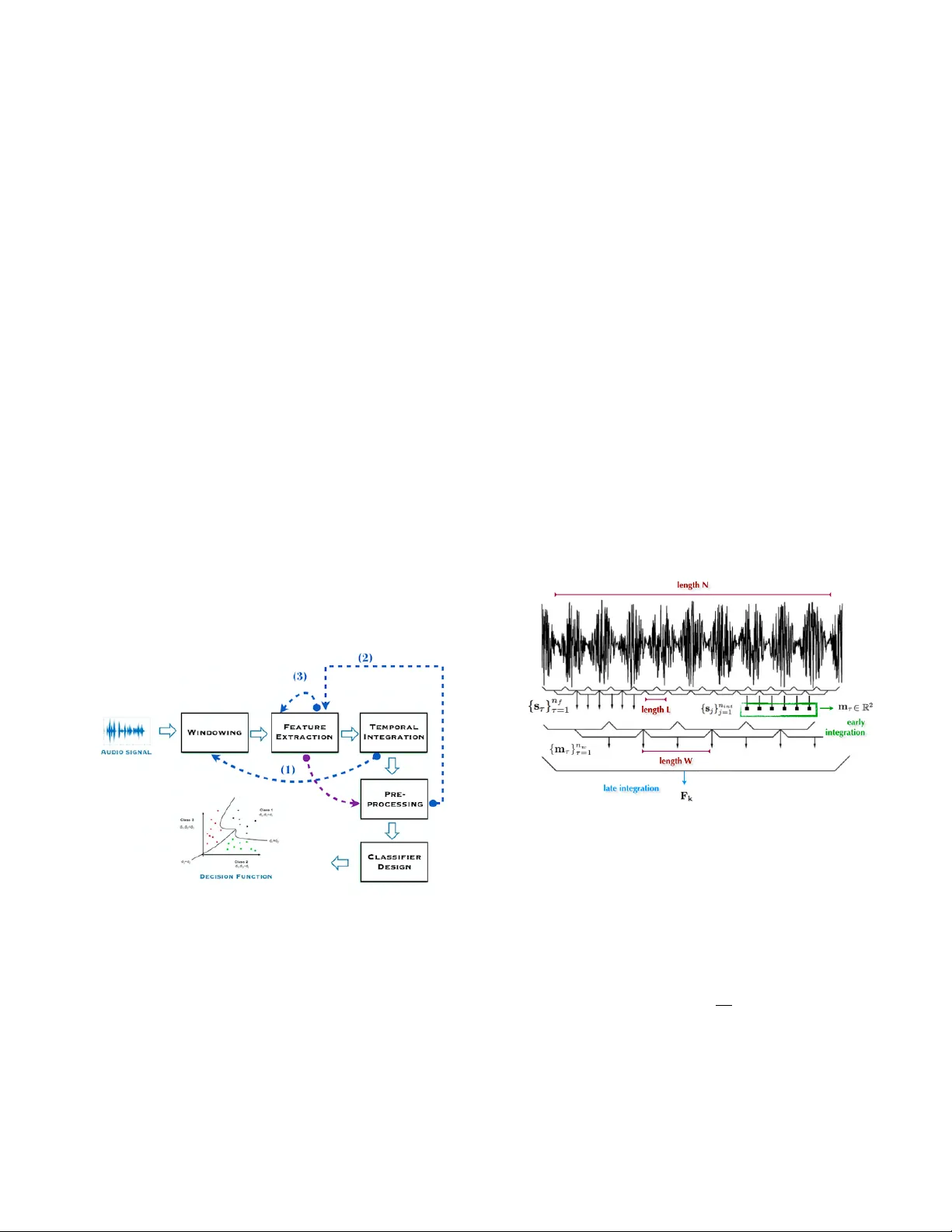
EXTENDED PIPELINE FOR CONTENT -B ASED FEA TURE ENGINEERING IN MUSIC GENRE RECOGNITION T ina Raissi † Alessandr o T ibo ‡ P aolo Bientinesi ∗ † † R WTH Aachen Uni versity , AICES, Schinkelstr . 2, 52062 Aachen, Germany ‡ Uni versity of Florence, Department of Information Engineering, V ia S. Marta 3, 50139 Firenze, Italy ABSTRA CT W e present a feature engineering pipeline for the constructi on of musical signal characteristics, to be used for the design of a supervised model for musical genre identification. The ke y idea is to extend the traditional two-step process of e xtraction and classification with additive stand-alone phases which are no longer or ganized in a waterf all scheme. The whole system is realized by tra versing backtrack arrows and c ycles between various stages. In order to gi ve a compact and effecti ve repre- sentation of the features, the standard early temporal inte gra- tion is combined with other selection and extraction phases: on the one hand, the selection of the most meaningful char - acteristics based on information gain , and on the other hand, the inclusion of the nonlinear correlation between this subset of features, determined by an autoencoder . The results of the experiments conducted on GTZAN dataset re veal a noticeable contribution of this methodology to wards the model’ s perfor- mance in classification task. Index T erms — Musical signal, genre classification, fea- ture extraction and selection, information gain, autoencoder 1. INTR ODUCTION One of the current subjects of research in Computer Science and Engineering concerns the enhancement of machines with abilities which are related to the human perception of the en vi- ronment. Since recently , the term machine hearing [1] is used as an umbrella to unify all applications of speech, music and en vironment sounds processing under a general concept. The central goal of this field is to model the hearing apparatus and its internal functionality [2]. Ho wev er , in the case of speech and music, it is not possible to achie ve this goal without tak- ing into account the representation of intrinsic characteristics of the sound, developed in relation to the relati ve learning task. In our case, the quality of the musical signal features is e valuated with respect to the task of genre classification, a well-established, and rather controversial topic of Musical Information Retriev al. A quick look-back at remarkable works [3] shows that the ∗ Financial support from the Deutsche Forschungsgemeinschaft (DFG) through grant GSC 11 is gratefully acknowledged. signal representation is obtained by the extraction of physical and perceptual features, in time, frequency and cepstral do- mains. This solution carries out the transformation of the orig- inal input signal to a new feature space. A reduction which results to be problematic, because the conservation of the rel- ev ant traits of the former is not guaranteed. This loss of infor- mation is caused by the applied analytical and computational model, and at the same time, by the rigid order of different steps of construction of the whole system. W e shifted for this reason our attention from the analytical approach to a method- ological one, by presenting a new feature e xtraction pipeline. For some of the stages, our pipeline b uilds on existing meth- ods in its isolated stages. W e expanded the content-based fea- tures by adding the bottleneck layer’ s features of an autoen- coder , which forces to learn a lo w dimensional representation of the data. Moreover , the selection of the most predictive at- tributes, based on information gain criteria, is done by using a Random F or ests classifier trained on an intermediate lev el feature vector . The entire process is not actually designed for recovering the lost information during the reduction, but for enriching the resulting feature v ector with additi ve knowl- edge, useful for the specific classification task. The mean ac- curacy of the classifier, trained with the output dataset of this pipeline, is improv ed from the 78% to 91%. In the following sections, we first introduce the general structure of this pipeline and describe e very single process; we then present an ev aluation of effecti veness of the features, at both final and intermediate stages. 2. GENERAL PIPELINE For the most part, the proposed approaches in the literature for the automatic music genre identification, take into con- sideration a two-step process of extraction and classification, performed in consecuti ve order . In our work, the intermediate stages of the extraction gain autonomy , and can be reached from later stages. In this section we giv e a concise description of the process. As shown in Figure 1, the input of the process is a con- tinuous audio stream. The extraction of information from the digitalized audio signal is generally carried out by algorithms operating on prefixed time windo w or consecuti ve blocks of frames. In order to obtain a vector F ∈ R 2 relativ e to one feature, we should perform the stages windowing, feature e x- traction and temporal integration twice, by using the back- track arro w (1). The first loop is responsible for the extraction of the short-time featur es , while the second loop is concerned with the extraction of medium-time features and the tempo- ral integration over the whole signal length. In both cases we hav e an early temporal integration [4] which uses the Mean- V ar model [5]. In Figure 1, the arrow (3) refers to the extraction of deriv a- tiv es after the first windo wing step. The feature vector ex- tracted at this level can already be used for a classification task. In contrast to many existing approaches, we use this fea- ture vector not for the final task, but for an intermediate classi- fier , built by random forests. The measure of the contribution of each attribute to the prediction of the target class is calcu- lated by summing the information gain of each attrib ute, at ev ery split. The attributes with positi ve contrib ution are then selected. In the pipeline, this step is indicated as preprocess- ing and is follo wed by another feature extraction step, con- nected via the backtrack arro w (2). This final extraction uses an autoencoder which maps the vector of selected features to itself. The features selected from the bottleneck layer are not going to substitute the original dataset, but are added to it, as an additional information about nonlinear correlation be- tween features. As a last step before the training phase, the dataset is normalized. Fig. 1 . The general pipeline for content-based feature engi- neering, with backtracking and forward arro ws. 3. FEA TURE EXTRA CTION AND T AXONOMY 3.1. Content-based features W e used three main categories of content-based features, based on a taxonomy presented in [6]: T ime Domain Phys- ical, Frequency Domain Physical and Cepstral Domain Per- ceptual. Following the three basic requirements of musical characteristics introduced by [4], we are interested in obtain- ing a single v alue or a low-dimensional vector , from sev eral feature observ ations, known also as early temporal integra- tion method. W e use the MeanV ar model, which calculates mean and standard deviation of observed v alues within a prefixed textur e window [7]. The early temporal integration procedure is illustrated in Figure 2: first, 14 features are extracted by using an analysis frame [7] of 50 milliseconds with 50% overlapping. Namely , Compactness, Energy , En- tropy of Energy , Root Mean Square (RMS), Zero Crossing, 26 Mel Frequency Cepstral Coefficients (MFCC), Chroma vector corresponding to 12 semitones, the standard deviation of v alues of Chroma vector , 10 Linear Prediction Coefficients (LPC), Spectral Centroid, Spectral Flux, Spectral Rolloff, Spectral Spread and Spectral V ariability . The computation of deriv atives and a temporal integration step ov er both feature values and their deri vati ves follow . The Fraction of Lo w En- ergy W indows (F oLEW) is then determined, and a conclusi ve temporal inte gration step is performed. Finally , from the Beat Histogram the Beat Sum, Strongest Beat (SBeat), Strength of Strongest Beat (SSBeat), and their deriv atives are extracted. The computation of all these features is detailed in [8]. Fig. 2 . The temporal inte gration procedure relati ve to the ex- traction of one feature vector . 3.2. Early temporal Integration As a first step, the signal is di vided into n f analysis frames of length L . For every feature, a vector s ∈ R n f of short- time values is extracted. In the second step, the mean and the standard deviation of n int = n f n w values of the vector s corresponding to a texture window of length W is calcu- lated. Consequently , for e very feature we have a matrix of medium-time values, having two ro ws deri ved from concate- nation of m τ = [ µ τ , σ τ ] T , ∀ τ = 1 , · · · , n w . The feature vec- tor F k ∈ R 2 is the a verage v alue of e very row of the medium- time matrix, corresponding to the k -th feature. 3.3. Bottleneck layer’ s features The linear version of Principal Component Analysis (PCA) is a common learning method for analyzing and gi ving a lo w- dimensional representation of an input space [9]. A generalization of PCA can be obtained by using an au- toencoder [10], which is a pair of stacked neural networks : an encoder E and a decoder D . The encoder maps an input data x ∈ R n into a hidden vector E ( x ) = h ∈ R d with typically d  n . The decoder maps h to an output vector x 0 ∈ R n . The autoencoder is trained to copy the input x to D ( E ( x )) = x 0 by using binary cross-entropy loss function: L ( x , D ( E ( x ))) = −  x log( x 0 ) + ( 1 − x ) log( 1 − x 0 )  . If the data lies in a low dimensional manifold, the autoen- coder can actually learn such representation. Concerning mu- sic, we capture the ev olution of the musical content in the sig- nal by concatenating features referred to adjacent frames. The number of feature vectors that come from musically sound frames, is reasonably a subset of the whole feature space. Encoder Decoder E D h = E ( x ) x 0 = D ( E ( x )) x Fig. 3 . The architecture of a symmetric autoencoder . The encoding and decoding functions in an autoencoder has respecti vely n e and n d hidden layers, and in our case n e = n d . In addition to just mentioned n e + n d hidden lay- ers, we hav e also a middle layer kno wn as bottlenec k layer which tak es as input E ( x ) . An example of an autoencoder is depicted in Figure 3. 3.4. Featur e selection The notion of information gain is relati ve to the a verage v ari- ation of information entropy due to current state’ s changes. Of particular interest is the application of this concept in de- cision tr ees [11]. Generally speaking, the process of construc- tion of a decision tree is based on the choice of the attribute with highest IG, on whose values the dataset of ev ery node is split. In the feature selection process based on IG, ev ery ex- ample is considered as a vector of values containing a specific information for predicting the class. W e can construct a deci- sion tree and determine the I G i of i -th attribute or feature by P | nodes | j =1 I G i j , where I G i j is the information gain obtained by splitting on i -th attribute at j -th node. The idea of ranking I G i values is equi valent to establishing an importance order of features, concerning their contribution to the prediction. Giv en a set of training examples S , with |S x i = a | |S j | we de- note the fraction of examples of the i -th attrib ute having v alue a at j -th node. W e define entropy as H ( S ) = − X c ∈ classes p c ( S ) log 2 p c ( S ) , where p c ( S ) is the probability of a training e xample to be- long to class c . Hence the information gain I G i j obtained by splitting on attribute x i at node j can be reformulated as I G ( S j , x i ) = H ( S j ) − X v ∈ values ( x i )   S j ( x i = v )   |S j | H  S j ( x i = v )  . This function measures the dif ference of entropies before and after splitting on the specific attribute. 4. CLASSIFICA TION W e consider tw o dif ferent classifiers as final models: the Sup- port V ector Machines with both radial basis and linear ker- nels, and Random F or ests for the feature selection step at in- termediate stage of the pipeline. The choice of the latter, in- stead of a straightforward decision tree, deri ves from its well- known property of a voiding the ov erfitting problem. 5. EXPERIMENT The audio dataset is GTZAN [7], consisting of 1000 audio tracks, each 30 seconds long and associated to one of ten gen- res: blues, classical, country , disco, hiphop, jazz, metal, pop, reggae and rock. Exactly 100 tracks are associated to e very genre. All tracks were con verted in 22,050 Hz mono 16-bit wa v format. W e ran 10 experiments splitting the dataset into 900 samples of training set and 100 samples of test set, pre- serving the percentage of samples for each class. Feature se- lection and hyperparameter optimization of SVM are done by 10-fold cross v alidation on the training set. F or the extraction of content-based features, we used pyAudioAnalysis and jAu- dio [12, 13]. The analysis frame for short-time features and the te xture windo w for the medium-time features were set to 50 milliseconds and 1 second, respectively . In both cases we operated a 50% of overlap. After the feature selection in the preprocessing step, we dropped all feature components which resulted in no information gain. T able 1 lists the selected fea- tures with their dimensionality corresponding to the experi- ment with the best result. For the architecture of the autoencoder , summarized in T able 2, we used three stacked hidden layers of size 60, 20, 60 respectiv ely , with PReLU [14] activ ation, initialized using He normal initializer [15]. The first two hidden layers were fol- lowed by a Dropout [16] layer with probability 0 . 2 . Finally an output layer of size 190 with sigmoid activ ation, initial- ized using He uniform initializer , was stacked at the end of the network. The model w as trained by minimizing the bi- nary cross-entropy error loss. The autoencoder was fed with 900 training feature v ectors of size 190, rescaled in [0 , 1] . W e ran 100 epochs of the Adadelta [17] optimizer with learning rate 1.0, ρ = 0 . 95 ,  = 1 e − 08 without decay factor on mini- batches of size 32. Even though we did not have sufficient resources for an automatic hyperparameter optimization, the proposed structure minimizes the loss function on the train- ing set. The final dataset consisted of content-based features of T able 1 augmented with bottleneck layer’ s features. Before the classification step the whole dataset was rescaled in [0 , 1] . The best final classifier , trained over this dataset, turned out to be the SVM with radial basis k ernel. The h yperparameters of SVM resulted to be γ = 2 − 6 and C = 4 . T able 1 . The content-based features and their dimension- ality . For ev ery feature, mean (M), standard deviation (SD), mean of deriv ativ es ( ∆ M) and standard deviation of deriv a- tiv es ( ∆ SD) are reported. The symbol ” ? ” indicates the elim- ination of feature components (see Section 3 for the original dimensions) and ” - ” means that no feature was extracted. Featur es M SD ∆ M ∆ SD T otal Compactness 1 1 1 1 4 Energy 1 1 1 1 4 Entropy of Ener gy 1 1 - - 2 FoLEW 1 1 1 1 4 RMS 1 1 1 1 4 Zero Crossing 1 1 1 1 4 SBeat 1 1 1 1 4 SSBeat 1 1 1 1 4 Beat sum 1 1 1 1 4 MFCC 22 ? 22 ? 15 ? 26 85 Chroma V ector 11 ? 11 ? - - 22 SD of Chroma 1 1 - - 2 LPC 9 ? 9 ? 0 ? 10 28 Spectral Centroid 1 1 0 ? 1 3 Spectral Flux 1 1 1 1 4 Spectral Rolloff 1 1 1 1 4 Spectral Spread 1 1 1 1 4 Spectral V ariability 1 1 1 1 4 T able 2 . Autoencoder architecture. Layer #Nodes Dense, PReLU, Dropout(0.2) 60 Dense, PReLU, Dropout(0.2) 20 Dense, PReLU 60 Dense, Sigmoid 190 6. RESUL TS In the Music Information Retriev al Ev aluation eXchange (MIREX) 2012, the state of the art systems for 10 genre cat- egories achieved an accuracy of 50-80% [8]. T able 3 shows notable results in the literature. Regarding our approach, we measured the mean accuracy over ten e xperiments, at differ - ent stages of our pipeline: after the e xtraction of the content- based features, as the output of two cycles of windowing, feature extraction and early temporal integration steps, we obtained a mean accuracy of 78 %. The preprocessing step of feature selection increased this result to the 86 . 30 %. At the third and final stage, by performing an additional fea- ture extraction step with autoencoder , we achieved 91 %, thus surpassing the accuracy of all other approaches. T able 3 . Notable classification accuracies achie ved in the lit- erature for musical genre classification. Reference Accuracy Our approach 91 . 00 % Our approach, no bottleneck features 86 . 30 % Sturm et al. [18] 83 . 00 % Bergestra et al. [19] 82 . 50% Li et al. [20] 78 . 50 % Panagakis et al. [21] 78 . 20 % Lidy et al. [22] 76 . 80 % Benetos et al. [23] 75 . 40 % Holzapfet et al. [24] 74 . 00 % Tzanetakis et al. [7] 61 . 00 % 7. CONCLUSIONS W e introduced a ne w feature engineering pipeline for the au- tomatic identification of musical genre. In order to integrate the loss of information during the feature extraction, we reor - ganized the rigid waterf all scheme of the traditional tw o-step process of extraction and classification. W e maintained con- tinuity with respect to existing approaches in dif ferent funda- mental aspects, like temporal integration method and feature taxonomy . Simultaneously we carried out a feature selection method based on information gain and extended the content- based features with bottleneck layer’ s features of an autoen- coder . Neither of the two methods has ev er been applied on the feature vectors extracted from the musical signal. Thank to the feature selection stage, our system achie ved 86.30% of accuracy . The extension of the preprocessed feature vec- tors with the bottleneck features had a further contribution of 4.7% to the accuracy of the final model, which resulted to be 91%. If we take into account the semantic ambiguity every genre recognition system must deal with, the results we ob- tained open new insights for the future works on definition and construction of genre and sub-genre identification sys- tems, with an accuracy which can reach human performance. 8. REFERENCES [1] Richard F L yon, “Machine hearing: An emerging field [exploratory dsp], ” IEEE signal pr ocessing magazine , vol. 27, no. 5, pp. 131–139, 2010. [2] Da vid Gerhard, Audio signal classification: History and curr ent techniques , Department of Computer Science, Univ ersity of Regina, 2003. [3] Bob L Sturm, “ A surve y of e valuation in music genre recognition, ” in International W orkshop on Adaptive Multimedia Retrieval . Springer , 2012, pp. 29–66. [4] Cyril Joder , Slim Essid, and Ga ¨ el Richard, “T emporal integration for audio classification with application to musical instrument classification, ” IEEE T ransactions on Audio, Speech, and Language Pr ocessing , vol. 17, no. 1, pp. 174–186, 2009. [5] Anders Meng, Peter Ahrendt, Jan Larsen, and Lars Kai Hansen, “T emporal feature inte gration for music genre classification, ” IEEE T ransactions on A udio, Speech, and Language Processing , vol. 15, no. 5, pp. 1654– 1664, 2007. [6] Francesc Al ´ ıas, Joan Claudi Socor ´ o, and Xa vier Se vil- lano, “ A revie w of physical and perceptual feature ex- traction techniques for speech, music and en vironmental sounds, ” Applied Sciences , vol. 6, no. 5, pp. 143, 2016. [7] Geor ge Tzanetakis and Perry Cook, “Musical genre classification of audio signals, ” IEEE T ransactions on speech and audio pr ocessing , vol. 10, no. 5, pp. 293– 302, 2002. [8] Alexander Lerch, An intr oduction to audio content anal- ysis: Applications in signal pr ocessing and music infor- matics , John Wile y & Sons, 2012. [9] Ian T Jollif fe, “Principal component analysis and factor analysis, ” in Principal component analysis , pp. 115– 128. Springer , 1986. [10] DE Rummelhart and JL McClelland, “P arallel dis- tributed processing, v ol. 1: Foundations, ” 1986. [11] T om M Mitchell, “Machine learning. 1997, ” Burr Ridge, IL: McGraw Hill , v ol. 45, no. 37, pp. 870–877, 1997. [12] Theodoros Giannakopoulos, “pyaudioanalysis: An open-source python library for audio signal analysis, ” PloS one , vol. 10, no. 12, pp. e0144610, 2015. [13] Cory McKay , Ichiro Fujinaga, and Philippe Depalle, “jaudio: A feature extraction library , ” in Proceedings of the International Conference on Music Information Retrieval , pp. 600–3. [14] Andre w L Maas, A wni Y Hannun, and Andrew Y Ng, “Rectifier nonlinearities improve neural network acous- tic models, ” in Proc. ICML , 2013, v ol. 30. [15] Kaiming He, Xiangyu Zhang, Shaoqing Ren, and Jian Sun, “Delving deep into rectifiers: Surpassing human- lev el performance on imagenet classification, ” in Pr o- ceedings of the IEEE international confer ence on com- puter vision , 2015, pp. 1026–1034. [16] Nitish Sriv astav a, Geof frey E Hinton, Alex Krizhevsky , Ilya Sutske ver , and Ruslan Salakhutdinov , “Dropout: a simple way to pre vent neural networks from o verfit- ting., ” J ournal of machine learning r esear ch , v ol. 15, no. 1, pp. 1929–1958, 2014. [17] Matthe w D Zeiler , “ Adadelta: an adaptive learning rate method, ” arXiv preprint , 2012. [18] Bob L Sturm, “On music genre classification via com- pressiv e sampling, ” in 2013 IEEE International Confer- ence on Multimedia and Expo (ICME) . IEEE. [19] James Bergstra, Norman Casagrande, Dumitru Erhan, Douglas Eck, and Bal ´ azs K ´ egl, “ Ag gr egate features and adaboost for music classification, ” Machine learning , vol. 65, no. 2-3, pp. 473–484, 2006. [20] T ao Li, Mitsunori Ogihara, and Qi Li, “ A comparati ve study on content-based music genre classification, ” in Pr oceedings of the 26th annual international A CM SI- GIR confer ence on Resear ch and development in infor - maion r etrieval . A CM, 2003, pp. 282–289. [21] Ioannis Panagakis, Emmanouil Benetos, and Constan- tine K otropoulos, “Music genre classification: A multi- linear approach, ” in ISMIR , 2008, pp. 583–588. [22] Thomas Lidy , Andreas Rauber, Antonio Pertusa, and Jos ´ e Manuel Inesta, “Mirex 2007 combining audio and symbolic descriptors for music classification from au- dio, ” MIREX 2007 - Music Information Retrie val Eval- uation eXchange , 2007. [23] Emmanouil Benetos and Constantine K otropoulos, “ A tensor-based approach for automatic music genre clas- sification, ” in Signal Processing Confer ence, 2008 16th Eur opean . IEEE, 2008, pp. 1–4. [24] Andre Holzapfel and Y annis Stylianou, “Musical genre classification using nonne gativ e matrix factorization- based features, ” IEEE T ransactions on Audio, Speech, and Language Processing , v ol. 16, no. 2, pp. 424–434, 2008.