Angle-Based Sensor Network Localization

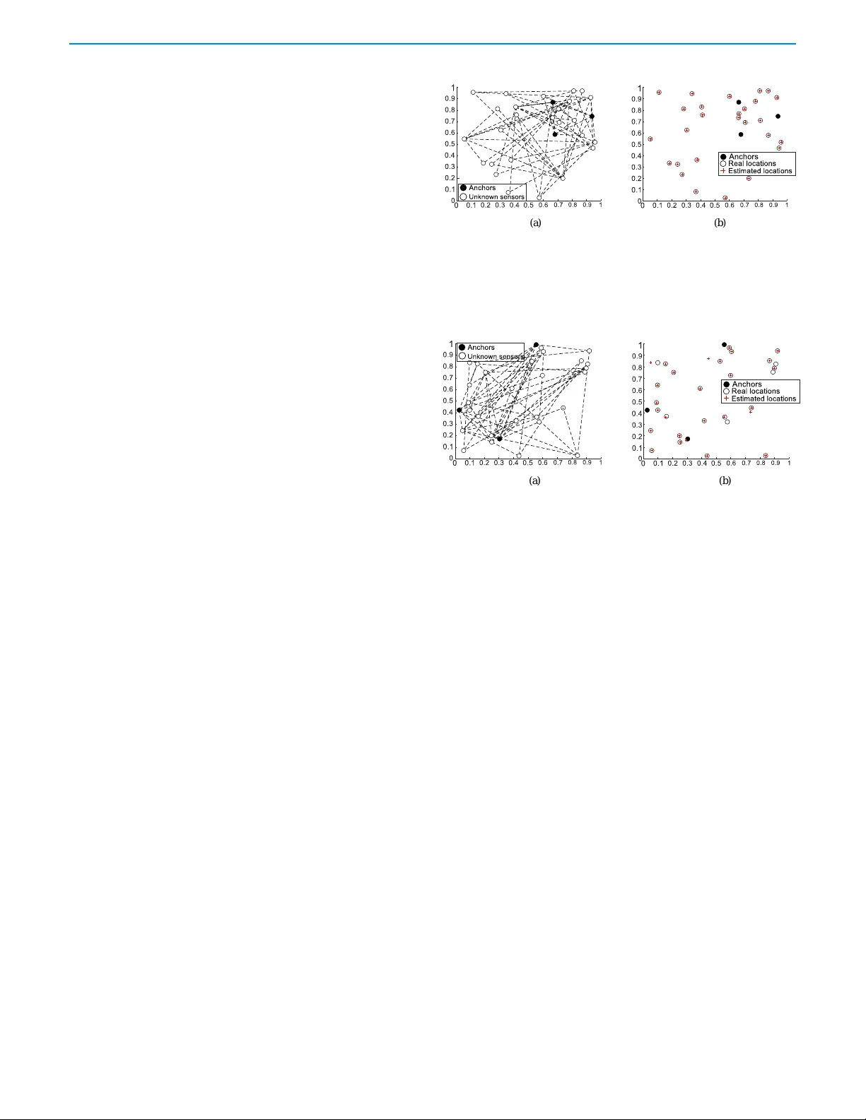
GENERIC COLORIZED JOURNAL, V OL. XX, NO . XX, XXXX 2020 1 Angle-Based Sensor Network Localization Gangshan Jing, Changhuang W an and Ran Dai Abstract — This paper studies angle-based sensor net- work localization (ASNL) in a plane, which is to determine locations of all sensors in a sensor netw ork, given loca- tions of par tial sensors (called anchors) and angle mea- surements obtained in the local coordinate frame of each sensor . Firstly it is shown that a framework with a non- degenerate bilateration ordering must be angle ﬁxable, im- plying that it can be uniquely determined by angles between edges up to translations, r otations, reﬂections and unif orm scaling. Then ASNL is pro ved to have a unique solution if and only if the grounded framew ork is angle ﬁxable and anchors are not all collinear . Subsequently , ASNL is solved in centralized and distributed settings, respectivel y . The centralized ASNL is f ormulated as a rank-constrained semi- deﬁnite program (SDP) in either a noise-free or a noisy scenario, with a decomposition approach proposed to deal with large-scale ASNL. The distributed protocol for ASNL is designed based on inter-sensor communications. Graph- ical conditions for equiv alence of the formulated rank- constrained SDP and a linear SDP , decomposition of the SDP , as well as the effectiveness of the distributed protocol, are proposed, respectively . Finally , simulation examples demonstrate our theoretical results. Index T erms — Network localization, angle rigidity , rank- constrained optimization, non-con vex optimization, chordal decomposition I . I N T R O D U C T I O N A sensor network localization problem is to determine lo- cations of all sensors when locations of partial sensors (called anchors) and relati ve measurements between some pairs of sensors are av ailable. It has received signiﬁcant attention due to the importance of sensor locations in many scenarios, e.g., fusion of sensor measurements according to locations, searching sensors in speciﬁed areas, and tracking a moving target [1], [2], [3]. In the literature, depending on sensing capabilities of sen- sors, sensor network localization (SNL) has been studied via relative position-based [4], range-based [1], [5]-[10] and bearing (angle of arriv al)-based [11]-[19] approaches. Among them, bearing-based SNL (BSNL) is a popular topic in recent years since bearings can be captured by vision sensors [16]. Nev ertheless, BSNL requires each sensor to know bearing measurements with respect to the global coordinate frame, This supplementary paper contains all the theoretical proofs missed in the journal paper “Angle-Based Sensor Network Localization”, which is published in IEEE T r ansactions on Automatic Control. Gangshan Jing and Changhuang W an are with Depar tment of Mechanical and Aerospace Engineering, The Ohio State Univer- sity , Columbus, OH 43210, USA. Emails: nameisjing@gmail.com and wan.326@osu.edu Ran Dai is with the School of Aeronautic and Astronautics, Purdue University , W est Lafa yette , IN 47907, USA. Email: randai@purdue.edu which can be realized by either equipping each sensor with speciﬁc devices (e.g., GPS, compasses) [12], [14] or imple- menting coordinate frame alignment algorithms [17], [19], [20] via inter-sensor communications. As a result, these meth- ods either become inv alid in GPS-denied en vironments (e.g., underwater , indoor) or require frequent inter-sensor commu- nications before or during implementation of the localization protocol. Although the authors in [15] proposed an algorithm based on bearings measured in local coordinate frames, the sensing graph has to contain more edges for solvability of SNL compared to localization via global bearing measure- ments (e.g., [12], [14]). In addition, extensi ve efforts have been carried out on range-based SNL (RSNL), where range measurements are independent of the global coordinate frame. Unfortunately , in many circumstances the solvability of RSNL requires more sensing than BSNL. In SNL problems, it is important to distinguish what kind of sensor network is localizable given av ailable anchor locations and measurements from sensors. This problem is usually tackled by checking whether the shape of the grounded graph can be uniquely determined by measurements. In BSNL and RSNL, bearing rigidity theory [11]-[19], [21], [22] and distance rigidity theory [1], [7], [10], [23]-[26] are employed to propose conditions for localizability , respecti vely . In [27], the authors ﬁrst dev eloped an angle-based shape determination approach (namely , angle rigidity theory), where the minimum number of edges required for shape determination is the same as that for the bearing-based approach. Note that an angle between two edges joining one sensor is independent of the global coordinate frame. In practice, bearing (angle) measurements in a local coordinate system are usually low cost, reliable, and can be captured by vision sensors (e.g., monocular pinhole cameras [29]). In recent years, angle-based formation control has attracted a gro wing interest due to the abov e-mentioned advantages of using angles as constraints or measurements [27]-[32]. Howe ver , the application of angle measurements to SNL has not been fully explored. Although a distributed SNL problem is equiv alent to a distributed formation control problem in special cases, they are generally different because sensors may not be subject to dynamics constraints 1 . In [33], angle measurements are utilized in SNL, but the proposed approach requires the network to have more sensing and communication links than being angle rigid. In the present work, SNL based on angle measurements will be 1 In this paper , we study SNL from an optimization perspective, where sensors are not considered to have speciﬁc dynamics on their estimated states. In the case when sensors are subject to dynamics constraints, the distrib uted SNL problem becomes ho w to solve the optimizations formulated in this paper in a multi-agent cooperativ e control setting. 2 GENERIC COLORIZED JOURNAL, V OL. XX, NO . XX, XXXX 2020 studied under a milder graphical condition than that in [27]- [33], and the proposed algorithms achie ve guaranteed global con vergence. SNL based on angle measurements is named angle-based sensor network localization (ASNL), which is to determine locations of the sensors other than anchors, given locations of anchors and angle measurements obtained in the local coordinate system of each sensor . In this paper , we propose the concept of angle ﬁxability based on angle rigidity theory in [27], [31] to characterize the property of a network that can be determined by angles uniquely up to translations, rotations, uniform scaling and reﬂections. By establishing connections between angle ﬁxa- bility and angle localizability , the results on angle ﬁxability are applied to ASNL problems. ASNL will be studied in centralized and distributed framew orks, respectively . In both centralized ASNL (CASNL) and distributed ASNL (D ASNL), each sensor is only capable of obtaining angle measurements with respect to its own local coordinate frame. A preliminary v ersion of the centralized case has been presented in [34]. This paper extends our former work in [34] by presenting the generic property of angle ﬁxability , chordal decomposition, ASNL with noises, DASNL and de- tailed proofs for Theorems 3 and 4. Our main contributions are summarized as follows: • Equiv alent algebraic conditions (Lemmas 2, 3) and a sufﬁcient graphical condition (Theorem 1) for angle ﬁx- ability in a plane are proposed. This graphical condition is milder than that in angle-based cooperative control references [27]-[33], and it implicitly implies an approach to constructing angle ﬁxable frameworks (Defnition 3). • A graphical condition for localizability of ASNL is given (Theorem 2). The CASNL problem is formulated as a rank-constrained semi-deﬁnite program (SDP) (Lemma 10). It is sho wn that if the grounded frame work is acute- triangulated, then ASNL is equiv alent to a linear SDP , which can be solved in polynomial time; see Theorem 5. • T o handle large scale ASNL problems, we formulate ASNL as an SDP with two unkno wn matrices (problem (8)). When the grounded graph has a bilateration order- ing, the ﬁrst unknown matrix can be decomposed via chordal decomposition (Theorem 7); when the grounded framew ork is acute-triangulated, the second unknown matrix can be decomposed into matrices in reduced sizes as well (Theorem 8). • In a noisy en vironment, from the maximum likelihood estimation perspecti ve, we model ASNL as an SDP with multiple rank-1 constraints and semi-deﬁnite constraints, which can be solved by algorithms in [36], [37], [40]. • Based on communications between adjacent sensors, a distributed protocol (Protocol 1) is proposed, which solves ASNL with guaranteed ﬁnite-time conv ergence (Theorem 10). The upper bound of the con vergence step is shown to be the number of sensors to be localized. The main advantages of the proposed ASNL approach can be summarized from the following two perspecti ves: (i) Com- pared with BSNL, each sensor does not need bearing informa- tion in the global coordinate frame. In [17], [19], [20], sensors obtain global bearing measurements by communicating with each other , which is a necessary procedure before or during implementation of the bearing-based localization algorithm. In constrast, the proposed CASNL approach does not require communications between sensors at all. Moreover , in D ASNL, the coordinate frame alignment procedure can be av oided, and each sensor only communicates with its neighboring sensors for ﬁnite times. Hence, the ASNL approach requires lo wer communication costs. (ii) Compared with RSNL, the angle- based approach is applicable to a set of SNL that cannot be resolved by the e xisting range-based approaches (e.g., examples in Fig. 1 (b), (c), (d), and Fig. 3). The outline of this paper is as follows. Section II provides preliminaries of angle rigidity theory and chordal decompo- sition. Section III introduces the concept of angle ﬁxability and provides criteria for angle ﬁxability and relev ant prop- erties. Section IV formulates ASNL as a QCQP and gives the necessary and sufﬁcient conditions for ASNL to hav e a unique solution. Section V solves the noise-free and noisy ASNL using a centralized framework. Section VI proposes a distrib uted protocol via inter-sensor communications for ASNL. Section VII exhibits sev eral simulation examples. The concluding remarks are addressed in Section VIII. Notation : Throughout the paper , G = ( V , E ) denotes an undirected graph, where V and E ⊂ V × V denote the vertex set and edge set, respecti vely . The neighbor set of each v ertex i is denoted by N i = { j ∈ V : ( i, j ) ∈ E } . A m × n zero matrix is denoted by 0 m × n , where “ m × n ” may be omitted if the dimension of the zero matrix can be observed. Giv en sets A and B , | A | is the cardinality of A , A \ B is the set of elements in A but not in B . The d -dimensional orthogonal group is written as O ( d ) . Giv en a matrix X , rank( X ) is the rank of X , X  0 implies that X is positive semi-deﬁnite, det( X ) denotes the determinant of X . A vector p = ( p > 1 , ..., p > s ) > is degenerate if p 1 , ..., p s are collinear . W e use K to represent a complete graph with appropriate number of vertices, I d to denote the d × d identity matrix, ⊗ to denote the Kronecker product, X a : b,c : d is the submatrix of X consisting of elements from a -th to b -th rows and c -th to d -th columns of X . Giv en matrices X and Y , h X, Y i = trace ( X > Y ) . I I . P R E L I M I N A R I E S In this section, some preliminaries of angle rigidity theory and chordal graphs will be introduced, which are important for studying solv ability and decomposability of an ASNL problem. A. Angle Rigidity Theor y In [27], angle rigidity theory is developed to study what kind of geometric shapes can be uniquely determined by angles subtended in the graph only . Similar to distance rigidity theory in RSNL and bearing rigidity theory in BSNL, angle rigidity theory plays an important role in solving ASNL. In [32], the authors presented a dif ferent angle rigidity theory by taking the sign of each angle into account, which implies that all angles are deﬁned in a common counterclockwise direction. Dif ferent from [32], the angle considered in this paper does not hav e a speciﬁc sign. As a result, different sensors are allowed to A UTHOR et al. : PREP ARA TION OF P APERS FOR IEEE TRANSA CTIONS AND JOURNALS (FEBR U AR Y 2017) 3 hav e different deﬁnitions about the rotational direction. In this subsection, we will brieﬂy re view several deﬁnitions regarding angle rigidity theory proposed in [27] that will be used later . A graph G = ( V , E ) with |V | = n can be embedded in a plane by giving each verte x i a position p i ∈ R 2 . The vector p = ( p > 1 , ..., p > n ) > ∈ R 2 n is called a conﬁguration , ( G , p ) is called a framework . Each angle we use to determine the framew ork shape is an angle between two edges joining one common vertex, and the cosine of this angle will be constrained. F or example, for the angle between edge ( i, j ) and ( i, k ) , the cosine of this angle, i.e., g > ij g ik , will be constrained, where g ij = p i − p j || p i − p j || is the bearing between vertices i and j . The set of angle constraints in a graph G can be denoted by { g > ij g ik = a ij k : a ij k ∈ [ − 1 , 1] , ( i, j, k ) ∈ T G } , T G = { ( i, j, k ) ∈ V 3 : ( i, j ) , ( i, k ) ∈ E , j < k } , here “ j < k ” avoids repeating each angle. Let θ ij k denote the angle between p i − p j and p i − p k , when a ij k is given, we can obtain a unique θ ij k = arccos a ij k ∈ [0 , π ] . That is, each angle constraint actually constrains an angle within the range [0 , π ] . Similar settings are considered in [28]-[31]. Note that when an angle is deﬁned under a speciﬁed counterclockwise direction, it should be within the range [0 , 2 π ) [32]. The angle rigidity function [27] of a framework ( G , p ) is deﬁned as f G ( p ) = ( ..., g > ij ( p ) g ik ( p ) , ... ) > , ( i, j, k ) ∈ T G . (1) A frame work ( G , p ) is globally angle rigid if f − 1 G ( f G ( p )) = f − 1 K ( f K ( p )) , here K is the complete graph with the same verte x set as G . ( G , p ) is inﬁnitesimally angle rigid if all the inﬁnitesimal angle motions are trivial. Here, the inﬁnitesimal angle motion is a motion of the framework such that all angles in the framew ork (i.e., f G ( p ) ) are in variant, a motion is trivial if it is a combination of translations, rotations, and uniform scaling. An alternati ve condition for inﬁnitesimally angle rigidity in R 2 is rank( ∂ f G ( p ) ∂ p ) = 2 n − 4 . In [27], the deﬁnitions of global angle rigidity and inﬁnitesimal angle rigidity are based on existence of a subset of T G , which are actually equiv alent to our deﬁnitions here. Compared with bearing rigidity [14], distance rigidity [23], and weak rigidity [38], [39], the essential novelty of angle rigidity theory is that only subtended angles are used in the rigidity function. Three examples are presented in Fig. 1 to illustrate these deﬁnitions. In Fig. 1, frame works (a) and (e) are nonrigid. In framew ork (a), vertices 1, 2, 3 and 4 can move simultaneously to deform the shape while maintaining all subtended angles. In framew ork (e), vertices 4 and 5 can mov e freely along the line between 1 and 4 and the line between 2 and 5, respecti vely . Framew orks (b), (c) and (d) are globally and inﬁnitesimally angle rigid because the angles in each framework are suf ﬁcient to determine the entire shape uniquely; in Fig. 1 (f), since the graph is complete, the framework is globally angle rigid. It is not inﬁnitesimally angle rigid because vertex 2 can mov e freely along the line between vertices 1 and 3. B. Chordal Graphs and Chordal Decomposition A graph is said to be chor dal if each cycle with more than three vertices in this graph has a chor d . Here a chord is an edge 1 2 5 4 3 1 2 5 4 3 1 2 5 4 3 1 2 5 4 3 1 2 5 4 3 1 2 3 1 2 5 4 3 1 2 5 4 3 1 2 3 ( a ) ( b ) ( c ) ( a ) ( b ) ( c ) ( d ) ( e ) ( f ) Fig. 1. Some frame works (graphs) in the plane, frameworks (a)-(e) have the same conﬁguration but diff erent graphs. between two nonconsecutive vertices in the cycle. A clique C of a graph G = ( V , E ) is a subset of V such that each pair of vertices in C are adjacent. In Fig. 1, graphs (a) and (b) are not chordal, graphs (c)-(f) are all chordal. W e say a clique C is a s -point clique if |C | = s . A clique C is said to be a maximal clique if there is no other clique containing this clique. In Fig. 1 (c), there are 3 maximal cliques: C 1 = { 1 , 2 , 3 } , C 2 = { 1 , 3 , 4 } , C 3 = { 2 , 3 , 5 } . Given a maximal clique C , we deﬁne a transformation matrix Q C ∈ R |C |× n such that Q C η = ( η C (1) , ..., η C ( |C | ) ) > ∈ R |C | for any n -dimensional vector η = ( η 1 , ..., η n ) > ∈ R n , C ( i ) denotes the i -th element of C . Each element of Q C is deﬁned as: ( Q C ) ij = ( 1 , j = C ( i ) , 0 , otherwise . (2) The following lemma giv es a condition for equiv alence be- tween positive semi-deﬁniteness of a matrix and positive semi-deﬁniteness of its submatrices corresponding to maximal cliques. Lemma 1: [41] Giv en G = ( V , E ) as a chordal graph and a matrix X ∈ R |V |×|V | , let {C 1 , C 2 , ..., C p } be the set of its maximal clique sets. Then, X  0 if and only if Q C k X Q > C k  0 , k = 1 , ..., p . I I I . A N G L E FI X A B I L I T Y T o better understand what kind of geometric shapes can be uniquely determined by angles, we introduce the notion of angle ﬁxability in this section, which is stronger than global angle rigidity and inﬁnitesimal angle rigidity . The formal deﬁnition of angle ﬁxability is giv en below . Deﬁnition 1: A framew ork ( G , p ) is angle ﬁxable in R d if f − 1 G ( f G ( p )) = S p , where S p = { q ∈ R nd : q = c ( I n ⊗ R ) p + 1 n ⊗ ξ , R ∈ O ( d ) , c ∈ R \ { 0 } , ξ ∈ R d } . (3) From Deﬁnition 1, we observe that the set S p actually deﬁnes a set of conﬁgurations forming the same shape as the one formed by p . That is, if q ∈ S p , then q can be obtained from p by a combination of rotations, translations, uniform 4 GENERIC COLORIZED JOURNAL, V OL. XX, NO . XX, XXXX 2020 scaling and reﬂections. In this paper , we mainly focus on angle ﬁxability in R 2 . Since the deﬁnition of angle ﬁxability in R d with d ≥ 3 will be used in Lemma 8 and Theorem 3 that state important conditions for removing the rank constraint in ASNL (Theorem 5), angle ﬁxability is deﬁned in an arbitrary dimensional space in Deﬁnition 1. A. Equivalent Conditions f or Angle Fixability in R 2 The follo wing two lemmas gi ve two necessary and suf ﬁcient conditions for angle ﬁxability in R 2 . Lemma 2: In R 2 , ( G , p ) is angle ﬁxable if and only if it is globally and inﬁnitesimally angle rigid. Pr oof: The sufﬁciency has been pro ven in [27, Theorem 1], next we prove the necessity . Suppose that ( G , p ) is angle ﬁxable but not inﬁnitesimally angle rigid, then rank( ∂ f G ∂ p ) = s < 2 n − 4 . As a result, there exists a neighborhood of p in which f − 1 G ( f G ( p )) is a 2 n − s > 4 dimensional manifold, this conﬂicts with the fact that f − 1 G ( f G ( p )) = S p is a 4- dimensional manifold. F or global angle rigidity , since it al ways holds that f − 1 K ( f K ( p )) ⊂ f − 1 G ( f G ( p )) , it sufﬁces to prove f − 1 G ( f G ( p )) ⊂ f − 1 K ( f K ( p )) . For an y q ∈ f − 1 G ( f G ( p )) , we hav e q ∈ S p , then g > ij ( q ) g ik ( q ) = g > ij ( p ) g ik ( p ) for all i, j, k ∈ V . That is, ( G , p ) is globally angle rigid. Lemma 3: In R 2 , ( G , p ) is angle ﬁxable if and only if it is globally angle rigid and p is non-degenerate. Pr oof: Since the conﬁguration of an inﬁnitesimally angle rigid framew ork can never be degenerate, the necessity can be obtained by Lemma 2. Next we prov e sufﬁcienc y . Global angle rigidity implies that f − 1 G ( f G ( p )) = f − 1 K ( f K ( p )) , hence we only ha ve to sho w that there exists some subgraph G 0 of K such that ( G 0 , p ) is inﬁnitesimally angle rigid. W ithout loss of generality , let 1 , 2 , 3 be three vertices not lying collinear . W e start with the complete graph with vertices 1, 2, 3, which is angle ﬁxable. Note that for any 4 ≤ i ≤ n , there always exist two vertices j, k ∈ { 1 , 2 , 3 } such that p i − p j and p i − p k are not collinear . By adding verte x i and edges ( i, j ) , ( i, k ) for i = 4 , ..., n iterati vely , we obtain a new graph G 0 . Moreover , at each step during the generation, the conditions in Lemma 7 (will be proposed later with its proof independent of this lemma) are satisﬁed. Thus ( G 0 , p ) is angle ﬁxable. Combining Lemma 2 and Lemma 3, the follo wing lemma holds. Lemma 4: Consider a globally angle rigid framew ork ( G , p ) in R 2 , the following statements are equiv alent: (i) p is non-degenerate; (ii) ( G , p ) is inﬁnitesimally angle rigid; (iii) ( G , p ) is angle ﬁxable. B. Generic Angle Fixability In [27], the authors sho wed that both inﬁnitesimal angle rigidity and global angle rigidity are generic properties of the graph. That is, given a graph G , either for all generic conﬁgurations 2 p ∈ R 2 n , ( G , p ) is inﬁnitesimally (globally) angle rigid, or none of them is. Therefore, angle ﬁxability in 2 A conﬁguration p = ( p > 1 , · · · , p > n ) > ∈ R 2 n is generic if its 2 n coordinates are algebraically independent [27]. R 2 is a generic property of the graph due to Lemma 2. W e giv e the following deﬁnition and result. Deﬁnition 2: A graph G is generically angle ﬁxable in R 2 if ( G , p ) is angle ﬁxable for any generic conﬁguration p ∈ R 2 n . Lemma 5: If ( G , p ) is angle ﬁxable for a generic conﬁgu- ration p ∈ R 2 n , then G is generically angle ﬁxable in R 2 . W e also note that all generic conﬁgurations in R 2 form a dense space. Therefore, for a generically angle ﬁxable graph G , the set of all conﬁgurations p ∈ R 2 n such that ( G , p ) is not angle ﬁxable is of measure zero. Lemma 5, together with Lemma 3, imply that for a framework with a generic conﬁguration p ∈ R 2 n , angle ﬁxability and global angle rigidity are equiv alent. W e summarize this result in the following lemma. Lemma 6: A graph G is generically angle ﬁxable in R 2 if and only if it is generically globally angle rigid in R 2 . C . Recognizing Angle Fixable F rame wor ks In this subsection, a graphical approach to recognizing angle ﬁxable frameworks will be presented. Before showing that, we ﬁrstly present the following result for angle ﬁxable framew orks. Lemma 7: Giv en an angle ﬁxable framework in R 2 , after adding a node and two non-collinear edges connecting this node to two existing nodes, the induced framework is still angle ﬁxable in R 2 . Pr oof: Let ( G , p ) be the angle ﬁxable framework with n vertices, n + 1 be the added node, ( n + 1 , u ) and ( n + 1 , v ) be the two added edges, ( G 0 , p 0 ) be the induced framew ork. W e only need to verify f − 1 G 0 ( f G 0 ( p 0 )) = S p 0 in order to prove that ( G 0 , p 0 ) is still angle ﬁxable. Since it always holds that S p 0 ⊂ f − 1 G 0 ( f G 0 ( p 0 )) , it sufﬁces to show f − 1 G 0 ( f G 0 ( p 0 )) ⊂ S p 0 . For each q 0 ∈ f − 1 G 0 ( f G 0 ( p 0 )) , it must hold that q 0 = ( q > , q 0 n +1 > ) > ∈ R 2 n +2 , where q ∈ S p , q 0 n +1 satisﬁes g > i,n +1 ( q 0 ) g ij ( q 0 ) = g > i,n +1 ( p 0 ) g ij ( p 0 ) , i ∈ { u, v } , j ∈ N i . Next we sho w that g u,n +1 can be uniquely determined by q and f G 0 ( p 0 ) . Lemma 2 sho ws that ( G , p ) is inﬁnitesi- mally angle rigid. Then verte x u must ha ve at least tw o neighbors j 1 , j 2 such that p u − p j 1 and p u − p j 2 are not collinear . Denote A = ( g uj 1 , g uj 2 ) ∈ R 2 × 2 , then rank( A ) = 2 . Note that if we regard g u,n +1 = x = ( x 1 , x 2 ) > ∈ R 2 as unknown v ariables, we then hav e A > x = b , where b = ( g > u,n +1 ( p 0 ) g uj 1 ( p 0 ) , g > u,n +1 ( p 0 ) g uj 2 ( p 0 )) . Hence g u,n +1 ( p 0 ) can be uniquely determined by q and f G 0 ( p 0 ) . Similarly , g v ,n +1 can be uniquely determined by q and f G 0 ( p 0 ) . Since g u,n +1 and g v ,n +1 are not collinear , they hav e only one intersection point. As a result, q 0 n +1 can be uniquely determined. Note that there must exist ˜ q = ( q > , q > n +1 ) > ∈ S p 0 such that ˜ q ∈ f − 1 G 0 ( f G 0 ( p 0 )) , we then hav e q 0 = ˜ q ∈ S p . In two-dimensional (2D) space, it is well known that any minimally rigid framework is embedded by a Laman graph [25], which can be obtained by Henneberg constructions [21], [22], [26]. At each step of Henneberg construction, either one verte x and two new edges are added (named verte x addition), or one v ertex and three new edges are added, while an e xisting edge is remov ed (named edge splitting). By Lemma 7, the speciﬁed Henneberg vertex additions preserve angle ﬁxability A UTHOR et al. : PREP ARA TION OF P APERS FOR IEEE TRANSA CTIONS AND JOURNALS (FEBR U AR Y 2017) 5 A n c h o rs S e n s o rs t o b e l o c a l i z e d 1 2 3 1 2 3 4 1 2 3 4 5 1 2 3 4 5 6 Fig. 2. An example of non-degenerate bilateration ordering. in 2D space. In [8], a graph containing a subgraph induced by Henneberg vertex addition ([21], [22], [26]) is said to hav e a bilateration or dering . For framew orks generated by graphs with a bilateration ordering, we deﬁne the non-degenerate bilateration ordering as follows. Deﬁnition 3: (Non-degenerate Bilateration Ordering) A framew ork ( G b ( n ) , p ( n )) is said to hav e a non-de generate bilateration ordering if it can be generated by the following procedure: Starting with the 3-verte x framework ( G b (3) , p (3)) where p (3) is non-degenerate, ( G b ( i + 1) , p ( i + 1)) is obtained from ( G b ( i ) , p ( i )) by adding one vertex l and s ≥ 2 edges connecting l to existing vertices l 1 , ..., l s such that p l − p l j , j ∈ { 1 , .., s } are not all collinear . Fig. 2 shows an example of the non-degenerate bilateration ordering. From Lemma 7, we hav e the follo wing result. Theor em 1: In R 2 , if a frame work has a non-degenerate bilateration ordering, then it is angle ﬁxable. A strongly non-degenerate triangulated framework ( G t , p ) is a framew ork with a non-degenerate bilateration ordering where at each step when a vertex l is added to ( G t ( i ) , p ( i )) , two non-collinear edges connecting l to j and k such that ( j, k ) ∈ E t are added accordingly . In [27], ( G t , p ) is shown to be angle ﬁxable in R 2 . One can realize that a strongly non-degenerate triangulated frame work always has a non- degenerate bilateration ordering, but not vice versa. Fig. 1 (b) shows a framework with a non-degenerate bilateration ordering, while it is not a triangulated frame work, because vertices 3 and 5 are not adjacent. By generic property of angle ﬁxability , the following result holds. Cor ollary 1: A graph with a bilateration ordering is gener- ically angle ﬁxable in R 2 . An interesting fact is that ev en if the frame work generated by Deﬁnition 3 in R 2 is elev ated into a higher dimensional space, it is still angle ﬁxable. See the follo wing lemma. Lemma 8: Giv en a framework ( G b ( n ) , p ) with a non- degenerate bilateration ordering in R 2 , for any integer d ≥ 3 , ( G b ( n ) , ¯ p ) is angle ﬁxable in R d , where ¯ p = ( ¯ p > 1 , ..., ¯ p > n ) > , ¯ p i = ( p > i , 0 1 × ( d − 2) ) > ∈ R d . Pr oof: W e prove the result by showing that in R d , ev ery q ∈ f − 1 G b ( n ) f G b ( n ) ( ¯ p ) satisﬁes q ∈ S ¯ p . Note that 1 , 2 and 3 always form a non-degenerate triangle, and a triangle is always angle ﬁxable in any dimensional space (The shape of a non-degenerate triangle constrained by angles is in variant to the dimension of the space). Hence, there must hold that q i = c R ¯ p i + ξ for some appropriate c , R and ξ , i = 1 , 2 , 3 . Suppose originally we ha ve ( G b ( i ) , q ( i )) , where q ( i ) ∈ S p ( i ) for c , R and ξ . Next, we prove that in the following Henneberg vertex addition introduced in Deﬁnition 3, the position of the ne w vertex to be added can be uniquely determined by angle constraints and positions of existing vertices. Let l be the added verte x, ( l, j ) and ( l , k ) be the two non-collinear added edges, j 1 and j 2 are two neighbors of j in G b ( i ) and q j − q j 1 is not collinear with q j − q j 2 . From the angle constraints in volving j , we have g > j l ( q ) g j j 1 ( q ) = c j lj 1 and g > j l ( q ) g j j 2 ( q ) = c j lj 2 . Next we show g j l can be uniquely determined. Note that g > j l ( q ) g j j 1 ( q ) = g > j l ( q ) R g j j 1 ( p ) , g > j l ( q ) g j j 2 ( q ) = g > j l ( q ) R g j j 2 ( p ) , ¯ p s = ( p > s , 0 1 × ( d − 2) ) > for s = j, j 1 , j 2 . Denote R > g j l ( q ) by b = ( b 1 , .., b d ) > ∈ R d , g j j 1 ( p ) by ζ = ( ζ 1 , ζ 2 , 0 1 × ( d − 2) ) > , and g j j 2 ( p ) by η = ( η 1 , η 2 , 0 1 × ( d − 2) ) > . Then we have ζ > b = c j lj 1 , η > b = c j lj 2 , which is equiv alent to  ζ 1 ζ 2 η 1 η 2   b 1 b 2  =  c j lj 1 c j lj 2  . Since g j j 1 ( p ) and g j j 2 ( p ) are not collinear , b 1 and b 2 can be uniquely determined. Note that ( b 1 , b 2 , 0 1 × ( d − 2) ) > = g lj ( p ) , implying that b 2 1 + b 2 2 = 1 . Since || b || = 1 , we have b s = 0 , s = 3 , ..., d . Then g j l ( q ) = R b is uniquely determined. Similarly , g lk ( q ) is also unique. Recall that g j l and g lk are not collinear , they hav e a unique intersection point, i.e., q l . This completes the proof. The above lemma implies that the angle ﬁxability of a framew ork with a non-degenerate bilateration ordering in R 2 is in variant to space dimensions. Howe ver , it does not mean that any frame work generated by Deﬁnition 3 in R d is angle ﬁxable. I V . A N G L E - B A S E D S E N S O R N E T W O R K L O C A L I Z A T I O N In this section, the problem settings and the mathematical formulation for ASNL will be presented. The condition in terms of the sensing graph for an ASNL problem to hav e a unique solution will be proposed as well. A. Problem Formulation T o introduce the problem formulation of ASNL, we will explain how the sensor network is modelled; what kind of information each sensor senses; and how a general ASNL can be mathematically formulated, successi vely . 1) Sensor network modelling : Giv en a network of sensors index ed by V = { 1 , ..., n } = A ∪ S , where A = { 1 , ..., n a } , S = { n a + 1 , ..., n a + n s } . Sensors in A are called anchors , whose locations are a vailable. Sensors in S are called unknown sensors , whose locations are unknown and to be determined. An undirected graph G = ( V , E ) is used as the sensing graph interpreting the interaction relationships between sensors. Each sensor has the capability of sensing bearing measurements in its local coordinate frame from other neighboring sensors j ∈ N i . An ASNL problem in R d is to determine x i , i ∈ S when { x i ∈ R d : i ∈ A} and all the angles between edges in G are av ailable. In this paper , we will focus on the case with d = 2 . Let x = ( x > 1 , ..., x > n ) > . Note that for any two anchors i, j , ev en if ( i, j ) / ∈ E , we can still obtain ( x i − x j ) / || x i − x j || since we know the accurate values of x i and x j . Therefore, 6 GENERIC COLORIZED JOURNAL, V OL. XX, NO . XX, XXXX 2020 2 3 4 A B F ● Anchors ○ Unknown Sensors 5 C D E i j k 1 Fig. 3. A sensor network where the locations of unknown sensors can be determined by measured angles and given locations of anchors . it is reasonable to utilize all the angles in framew ork ( ˆ G , x ) , with ˆ G = ( V , ˆ E ) , ˆ E = E ∪ { ( i, j ) ∈ V 2 : i, j ∈ A} in solving SNL. In this paper , we call ( ˆ G , x ) the gr ounded framework , and use N = ( ˆ G , x, A ) to denote a sensor network. A simple example of ASNL is shown in Fig. 3, where the position of sensor 4 can be uniquely determined by cos ∠ A , cos ∠ B and cos ∠ C . More speciﬁcally , cos ∠ B and cos ∠ C determine the shape of the triangle formed by 1, 3 and 4, the distance between anchors 1 and 3 determines the size of this triangle, cos ∠ A determines the direction of the relativ e position between 1 and 4. Similarly , the position of sensor 5 can be uniquely determined by angles cos ∠ D , cos ∠ E and cos ∠ F . Note that both the locations of sensor 4 and sensor 5 cannot be determined by lengths of edges in Fig. 3, implying that the RSNL approach is not applicable to this example. 2) Sensing capability : In this paper , we consider that each sensor only senses relative bearing measurements from its immediate neighbors, which can be captured by vision-based sensors [29], [16]. Moreov er , we consider a GPS-denied en vi- ronment, in which each sensor has an independent coordinate system. As a result, each pair of sensors may have different understandings about their relativ e bearing. Such a setting is actually equiv alent to assuming that each sensor senses angles subtended at itself. 3) A QCQP formulation : Given a sensor network ( ˆ G , x, A ) in R 2 , let p = ( p > 1 , ..., p > n ) > ∈ R 2 n be the real locations of sensors. The ASNL problem can be modeled as the following quadratically constrained quadratic program (QCQP): ﬁnd x, d ij , ( i, j ) ∈ ˆ E s.t. ( x i − x j ) > ( x i − x k ) = a ij k d ij d ik , ( i, j, k ) ∈ T ˆ G || x i − x j || 2 = d 2 ij , ( i, j ) ∈ ˆ E x i = p i , i ∈ A (4) where a ij k = ( p i − p j ) > || p i − p j || ( p i − p k ) || p i − p k || is the angle information obtained from bearing measurements, T ˆ G = { ( i, j, k ) ∈ V 3 : ( i, j ) , ( i, k ) ∈ ˆ E , j < k } is the angle index set determining all the angles subtended in the framew ork, d ij is the distance between sensors i and j for ( i, j ) ∈ ˆ E . The kno wn quantities in (4) include: a ij k ∈ R for ( i, j, k ) ∈ T ˆ G , p i ∈ R 2 for i ∈ A ; the unknown variables in (4) are: x i ∈ R 2 for i ∈ S , d ij ∈ R for ( i, j ) ∈ ˆ E , i or j ∈ S . Note that QCQP (4) can actually describe ASNL in arbitrary dimensional space. 1 2 3 4 3 ' 4 ' 1 2 3 4 4 ' 1 2 3 4 5 ( a ) ( b ) ( c ) Fig. 4. (a) A sensor network that is not angle localizable, sensors 3 and 4 may be incorrectly localized as 3 0 and 4 0 . (b) A sensor network that is not angle localizable, sensor 4 may be localized as 4 0 . (c) An angle localizable sensor network. Remark 1: In (4), all the angles in a sensor network are taken into account for localization. From the example in Fig. 3, only partial angles are required to determine locations of unknown sensors. That is, (4) contains redundant angle infor- mation for localization. Therefore, T ˆ G in (4) can be reduced to its subset T ∗ ˆ G . When ( ˆ G , x ) is strongly non-de generate triangulated, [27, Theorem 7] gives a minimal set of angle constraints for determining angle ﬁxability of ( ˆ G , x ) , which is also sufﬁcient for network localization. W e make the follo wing assumption for problem (4). Assumption 1: Problem (4) is feasible; there are no sensors ov erlapping each other; all sensors are static. For an arbitrary sensor network, once the measured angles a ij k , ( i, j, k ) ∈ T ˆ G are exact, Problem (4) is feasible. All the results in this paper will be established on the premise that Assumption 1 is valid. In practice, it may be difﬁcult for measurements to be exact. Ho wev er , even when only a range for each angle is measured, the feasibility of (4) still holds by replacing the ﬁrst class of equality constraints with inequality constraints. More details are explained in Remark 3. B. Angle Localizability After formulating the ASNL problem as the QCQP (4), we striv e to answer the question in this subsection: what kind of sensor networks will make the ASNL problem hav e a unique solution? Deﬁnition 4: A sensor network is angle localizable if there is a unique feasible solution to (4). Fig. 4 shows three demonstrations for Deﬁnition 4. The following Lemma giv es a necessary condition for sensor networks to be angle localizable. Lemma 9: If the sensor network is angle localizable in R 2 , then anchors are not all collinear . Pr oof: Suppose that anchors are all collinear . W e discuss the following two cases: Case 1, all sensors are collinear . Then given any sensor i ∈ S , there must exist a constant δ > 0 , such that for y i = x i − δ x i − x j || x i − x j || , it holds that y i − x j || y i − x j || = x i − x j || x i − x j || for any j ∈ V . That is, all the unkno wn sensors cannot be uniquely localized. Case 2, not all the sensors are collinear . Let y ∈ R 2 be a unit vector perpendicular to the line determined by anchors. It can be veriﬁed that ( ¯ x i − ¯ x j ) > ( ¯ x i − ¯ x k ) = ( x i − x j ) > ( x i − x k ) for all ( i, j, k ) ∈ T ˆ G and || ¯ x i − ¯ x j || = || x i − x j || for all ( i, j ) ∈ ˆ E , where ¯ x i = p i for i ∈ A , ¯ x i = H y x i for i ∈ S , H y = I 2 − 2 y y > is the Householder transformation. A UTHOR et al. : PREP ARA TION OF P APERS FOR IEEE TRANSA CTIONS AND JOURNALS (FEBR U AR Y 2017) 7 Lemma 9 implies that at least 3 anchors are required for angle localizability of a network in R 2 . Note that for SNL based on bearings measured in the global coordinate frame [12], [14], [16], [17], the minimum number of anchors required for localizability in R 2 is 2. This is because the angle between tw o global bearings can be determined as clockwise or counterclockwise in the global coordinate frame. As we claimed before, each angle considered in this paper is totally measured in the local coordinate frame, and cannot be recognized as clockwise or counterclockwise in the global coordinate frame. Fig. 4 (a) shows a sensor network that is localizable by bearings in the global coordinate frame, but is not angle localizable. In Fig. 4 (b), the sensor network is not localizable since all anchors are collinear . The following theorem shows a connection between angle localizability and angle ﬁxability . Theor em 2: A sensor network N = ( ˆ G , x, A ) is angle localizable in R 2 if and only if ( ˆ G , x ) is angle ﬁxable and anchors are not all collinear . Pr oof: Sufﬁcienc y . Let y = ( y > 1 , ..., y > n ) > ∈ R 2 n be a solution to (4). Since ( ˆ G , x ) is angle ﬁxable, we hav e y = c ( I n ⊗ R ) x + 1 n ⊗ ξ for some c ∈ R \ { 0 } , R ∈ O (2) , ξ ∈ R 2 . Lemma 9 implies that there exist at least 3 anchors located non-collinear . W ithout loss of generality , let 1 , 2 , 3 be the three anchors. Then y i = x i , i = 1 , 2 , 3 and x 1 − x 2 = y 1 − y 2 = c R ( x 1 − x 2 ) . Since || R || = 1 , we hav e | c | = 1 . Therefore, R 0 , c R ∈ O (2) . Similarly , we hav e x 1 − x 3 = R 0 ( x 1 − x 3 ) . Let A = ( x 1 − x 2 , x 1 − x 3 ) ∈ R 2 × 2 , A must be of full rank. Then we can obtain R 0 = I 2 from A = R 0 A . Since x 1 = Y 12 = R 0 x 1 + ξ , we hav e ξ = 0 . As a result, y = x . Necessity . Lemma 9 has sho wn that anchors are not all collinear , we next prove angle ﬁxability of ( ˆ G , x ) . Consider y = ( y > 1 , ..., y > n ) > ∈ R 2 n such that y ∈ f − 1 ˆ G ( f ˆ G ( x )) , it sufﬁces to pro ve y ∈ S x . Note that the subgraph ˆ G a composed by vertices { 1 , ..., n a } and related edges is complete. Let x a = ( x > 1 , ..., x > n a ) > , y a = ( y > 1 , ..., y > n a ) > . From Lemma 3, ( ˆ G a , x a ) is angle ﬁxable, then y a ∈ S x a . Angle localizability implies that giv en y a , the rest of coordinates of y such that f ˆ G ( x ) = f ˆ G ( y ) can be uniquely determined. Since a suitable y is an element in S x , hence there must hold y ∈ S x . Combing Theorem 1 and Theorem 2, we obtain a graphical condition for angle localizability , see the following corollary . Cor ollary 2: A sensor network N = ( ˆ G , x, A ) is angle localizable in R 2 if ( ˆ G , x ) has a non-degenerate bilateration ordering, and anchors are not all collinear . Corollary 2 implies that Deﬁnition 3 can be used to con- struct angle localizable sensor networks. Similar approaches for generating bearing localizable networks can be found in [21], [22]. Remark 2: When there are no anchors in the network, i.e., A = ∅ , sensors’ locations can still be determined uniquely up to rotations, translations, uniform scaling and reﬂections by solving (4). In this scenario, Deﬁnition 4 can be modiﬁed by using S x ∗ as the unique solution set of (4), where x ∗ corresponds to actual locations of sensors. Due to absence of anchors, it holds that ˆ G = G . The centralized and distributed approaches that will be presented later can also be extended 2 3 4 A B F ● A n c h o r n o d e s ○ Se n s o r n o d e s t o b e d e t e r m in e d 5 C D E i j k Fig. 5. An illustration for CASNL. to the anchor-free case. V . C A S N L : A N O P T I M I Z A T I O N P E R S P E C T I V E In this section, a centralized optimization framew ork is proposed to solve ASNL. In the CASNL, the information sensed by all sensors (including anchors) will be collected in a central unit, and the ASNL problem will be solved by this central unit. An example to illustrate the centralized approach to ASNL is presented in Fig. 5, where each sensor has its local coordinate frame and transmits local bearing measurements to the central unit, and inter-sensor communications are not required. In this setting, the bearing-based approaches in [12], [14], [16], [17], [19] are not applicable because they require each sensor to either measure the bearing measurements in the global coordinate frame or transform local bearings to global bearings by communicating with neighbors. The signiﬁcance of studying CASNL can be generally sum- marized as follows: (i) CASNL does not require each sensor to communicate with other sensors or perform computation. (ii) A CASNL frame work contributes to pri vacy preserving: since only angle or bearing information is transmitted to the central unit once, the third party cannot obtain any sensor’ s position unless it detects all the sensed information and knows anchors’ positions. (iii) The CASNL and the D ASNL have different objectiv es in practice, thus ha ve different application scenarios. The goal of CASNL is to obtain all sensors’ locations at the central unit, based on which the next task is set in a centralized framew ork, while in D ASNL each sensor localizes itself. A. An SDP Formulation T o solve the ASNL problem (4) from a centralized per- spectiv e, we will establish a linear SDP formulation based on ASNL (4), and analyze the condition for equiv alence of them. Here, “equi valence” of tw o problems means that there is a one- to-one correspondence between the solution sets of them. The results in this subsection can be trivially extended to ASNL in higher dimensional space. Let X = ( x n a +1 , ..., x n a + n s ) ∈ R 2 × n s , Y =  I 2 X X > X > X  ∈ R (2+ n s ) × (2+ n s ) , ˜ d = ( ..., d l ij , ... ) > ∈ R m , D = ˜ d ˜ d > ∈ R m × m , m = | ˆ E | . 8 GENERIC COLORIZED JOURNAL, V OL. XX, NO . XX, XXXX 2020 Deﬁne e i ∈ R n s and E i ∈ R m as an n s -dimensional and an m -dimensional unit vector with the i -th entry being 1, respectiv ely . Then ASNL (4) is con verted into an SDP min Y ,D 0 s.t. ( f i − f j ) > Y ( f i − f k ) = a ij k E > l ij D E l ik , ( i, j, k ) ∈ T ˆ G , ( f i − f j ) > Y ( f i − f j ) = E > l ij D E l ij , ( i, j ) ∈ ˆ E , Y 1:2 , 1:2 = I 2 , Y  0 , D  0 , (5) where Y 1:2 , 1:2 is the second leading principal submatrix of Y , and f i ∈ R n s +2 is deﬁned as f i =  ( p > i , 0 1 × n s ) > , i ∈ A , ( 0 1 × 2 , e > i − n a ) > , i ∈ S . SDP (5) is formulated by transforming variables x and ˜ d in (4) to matrix v ariables Y and D . Since Y and D are uniquely determined by x and ˜ d , any solution of (4) corresponds to a solution of (5). Ho wever , the con verse may not hold. Before we study the condition for equi valence of (4) and (5), we ﬁrstly equiv alently transform (5) to a standard SDP with only one matrix variable. Denote Q ij k = 1 2  ( f i − f k )( f i − f j ) > + ( f i − f j )( f i − f k ) >  , Q ij = ( f i − f j )( f i − f j ) > , R ij k = 1 2  E l ik E > l ij + E l ij E > l ik  , R ij = E l ij E > l ij , then (5) can be equiv alently rewritten as min Y ,D 0 s.t. h Q ij k , Y i = a ij k h R ij k , D i , ( i, j, k ) ∈ T ˆ G , h Q ij , Y i = h R ij , D i , ( i, j ) ∈ ˆ E , Y 1:2 , 1:2 = I 2 , Y  0 , D  0 . (6) T o include both Y and D in one matrix v ariable, we further deﬁne Z =  Y 0 0 D  , Φ ij k =  Q ij k 0 0 0 m × m  , Ψ ij =  Q ij 0 0 0 m × m  , ¯ Ψ ij =  0 ( n s +2) × ( n s +2) 0 0 R ij  , ¯ Φ ij k =  0 ( n s +2) × ( n s +2) 0 0 R ij k  . Then (5) becomes min Z 0 s.t. h Φ ij k , Z i = a ij k h ¯ Φ ij k , Z i , ( i, j, k ) ∈ T ˆ G , h Ψ ij , Z i = h ¯ Ψ ij , Z i , ( i, j ) ∈ ˆ E , Z 1: n s +2 ,n s +3: n s +2+ m = 0 , Z n s +3: n s +2+ m, 1: n s +2 = 0 , Z 1:2 , 1:2 = I 2 , Z  0 . (7) Giv en a sensor network, after the angle information mea- sured by sensors is transmitted to the central unit, all the matri- ces in (7) except variable Z will be known. More speciﬁcally , T ˆ G and ˆ E are determined by measurements from sensors; Φ ij k and Ψ ij are determined by T ˆ G , ˆ E and positions of anchors; ¯ Φ ij k and ¯ Ψ ij are determined by T ˆ G and ˆ E , respecti vely; a ij k is the angle information based on measurements from sensors. In what follows, we will analyze the property of solutions of (7), and propose a condition for equiv alence of (4) and (7). Lemma 10: Let Z be a solution to (7), then rank( Z ) ≥ 3 . Pr oof: From the deﬁnition of Z , we hav e rank( Z ) = rank( Y ) + rank( D ) . Since Y is symmetric, and Y 1:2 , 1:2 = I 2 , we hav e Y =  I 2 Y 12 Y > 12 Y 22  with Y 12 ∈ R 2 × n s and Y 22 ∈ R n s × n s . Then rank( Y ) = rank( I 2 )+rank( Y 22 − Y > 12 Y 12 ) ≥ 2 . For matrix D , Assumption 1 implies that D l ij l ik is not a zero matrix. Then rank( D ) ≥ 1 . In conclusion, rank( Z ) ≥ 3 . From Z  0 , we obtain that Y 22  Y > 12 Y 12 , and D is nontrivial. Since there is no rank constraint for Z in (7), it is possible that the rank of a solution Z is greater than 3 . As a result, a solution of (7) may not correspond to a solution to (4). The follo wing lemma shows that by imposing a rank constraint on Z , SDP (7) becomes equiv alent to (4). Lemma 11: If the rank of every solution to (7) is 3 , then (7) is equiv alent to (4). Pr oof: Gi ven X as a solution to (4), it is obvious that the induced Z is a solution to (7). Next we prove that gi ven a solution Z (with rank 3 ) to (7), we can ﬁnd a unique solution X corresponding to Z such that X is a solution to (4). Again, consider Y =  I 2 Y 12 Y > 12 Y 22  with Y 12 ∈ R 2 × n s and Y 22 ∈ R n s × n s . Since rank( Z ) = 3 , from the proof of Lemma 10, we have rank( Y ) = 2 , implying rank( Y 22 − Y > 12 Y 12 ) = 0 , then Y 22 = Y > 12 Y 12 . Moreov er, rank( D ) = 1 , then there exists some vector ¯ d ∈ R | ˆ E | such that D = ¯ d ¯ d > . Since Z and D are in the desired forms, the constraints in (7) are equiv alent to those in (4). Let X = Y 12 , X must be the solution to (4). Lemma 11 implies that ASNL (4) can be equiv alently formulated as the SDP (7) with an rank constraint rank( Z ) = 3 , which is a non-conv ex optimization and generally NP-hard. Although extensiv e methods for rank-constrained optimization hav e been proposed in the literature, e.g., [10], [36], [37], they only guarantee local con vergence for general cases. That is, the initial guess gi ven to the algorithm needs to be suf ﬁ- ciently close to an optimal solution. Moreover , solving a rank- constrained optimization is usually time-consuming especially when the problem is of large size. In the next subsection, by utilizing some inherent properties of ASNL, we will deriv e a condition for removing the rank constraint on the unknown matrix Z . Remark 3: By incorporating the rank condition in Lemma 11, the SDP formulation (7) is equiv alent to the original ASNL and is scalable to noises and bounded unknown disturbances. For example, in speciﬁc scenarios, each angle constraint is obtained within a range due to the existence of noises or disturbances, i.e., a ij k ∈ [ l ij k , u ij k ] , ( i, j, k ) ∈ T ˆ G . In this case, the ﬁrst class of equality constraints can be revised as A UTHOR et al. : PREP ARA TION OF P APERS FOR IEEE TRANSA CTIONS AND JOURNALS (FEBR U AR Y 2017) 9 inequality constraints l ij k h ¯ Φ ij k , Z i ≤ h Φ ij k , Z i ≤ u ij k h ¯ Φ ij k , Z i , ( i, j, k ) ∈ T ˆ G . Under this setting, when the sensing graph has a suf ﬁcient amount of edges, SDP (7) can still be solved with high accu- racy . An example (Example 5) will be giv en to demonstrate this fact in the simulation section. Moreover , the discussions on SDP (7) in the following two subsections are applicable to the case with bounded unknown disturbances as well. B. Relation to SDP Relaxation Since a rank-constrained SDP is difﬁcult to solve, we consider ho w to relax the rank-constrained SDP to a con ve x problem (i.e., remove the rank constraint). In the literature, e.g., [5], [6], [9], SDP relaxation has been widely used to solve RSNL. Howe ver , usually a solution to the relaxed problem may not correspond to a solution to the original problem. In this subsection, we will establish connections between the relaxed formulation in (7) and the original noncon vex QCQP in (4). The following theorem shows that under a speciﬁc graph condition, the rank of Z can be efﬁciently constrained once the rank of D is constrained. Theor em 3: Let Z = ( Y 0 0 D ) be a solution to (7) and rank( D ) = 1 , then rank( Z ) = 3 must hold if and only if (i) anchors are not all collinear; (ii) ( ˆ G , x ) is angle ﬁxable in R 2 and its angle ﬁxability is in variant to space dimensions. Pr oof: See Appendix. W e say a triangulated framework ( G , p ) is acute- triangulated if each triangle in this frame work only contains acute angles, i.e., for any ( i, j ) , ( i, k ) , ( j, k ) ∈ E , it holds that g > ij g ik , g > j i g j k , g > ki g kj ∈ (0 , 1) . As a result, an acute- triangulated framework must be strongly non-degenerate, and has a non-de generate bilateration ordering. Next we gi ve a graph condition for constraining the rank of D . Theor em 4: Let Z = ( Y 0 0 D ) be a solution to (7). If ( ˆ G , x ) is acute-triangulated, then rank( D ) = 1 . Pr oof: See Appendix. Remark 4: In simulation experiments, by solving the SDP formulation in (7), all unknown sensors can always be cor- rectly localized when ( ˆ G , x ) is strongly non-degenerate trian- gulated. W e will make further efforts to prov e this in future. Howe ver , when ( ˆ G , x ) has a non-de generate bilateration order - ing but is not triangulated, the solution to (7) may correspond to incorrect localization results. An example (Example 2) will be given in Section VII. By virtues of Theorems 3, 4 and Lemma 8, the follo wing result is deriv ed. Theor em 5: Given a sensor network N = ( ˆ G , x, A ) , if ( ˆ G , x ) contains an acute-triangulated subframework, and an- chors are not all collinear , then (i) (4), (5), (6) and (7) are all equi valent; (ii) (7) has a unique solution with rank 3. The conclusions in Theorem 5 imply that ASNL is angle localizable, and QCQP (4) is equiv alent to its SDP relaxation, thus can be ef ﬁciently solved within polynomial time. (4)=(7) rank(Z)=3 rank(D)=1 acute triangulated non-degenerate bilateration ordering angle f i x a bility - Fig. 6. The relationships between different conditions f or the grounded framew or k and relaxation results. Anchors are always considered to be not all collinear . T o clearly demonstrate the results stated in Theorems 3, 4 and 5, we summarize the relationships between dif ferent conditions for ( ˆ G, x ) and relaxation results in Fig. 6. Here we assume that anchors are always not all collinear . C . Decomposition f or Large-Scale ASNL The formulation in (7) is a standard linear SDP , thereby can be globally solv ed by the interior-point methods in polynomial time. Howe ver , when the dimension of Z is very large, due to high computational costs of considering the positive semi- deﬁnite constraint, existing interior-point algorithms may be unable to ﬁnd the solution within reasonable computational time. Note that large-scale networks are ubiquitously encoun- tered in practice. From intuitiv e observation, when the sensor network is of large scale, matrices Φ ij k , ¯ Φ ij k , Ψ ij and ¯ Ψ ij in (7) are usually large and sparse. In this subsection, we will recognize some special features of ASNL and transform a large and sparse ASNL to a linear SDP with multiple semi- deﬁnite cone constraints for smaller-sized matrices. It is observed that compared to (7), the problem in (6) has a smaller size and fewer constraints. Therefore, we will focus on problem (6) directly . By Theorem 3, the original ASNL (4) is equiv alent to the following SDP: min Y ,D 0 s.t. h A i , Y i + h B i , D i = c i , i = 1 , ..., s, Y , D  0 , rank( D ) = 1 , (8) where A i ∈ R ( n s +2) × ( n s +2) , B i ∈ R m × m , s = |T ˆ G | + | ˆ E | + 4 . 1) Decomposition for Y : Due to the deﬁnition of the inner product for matrices, an entry in Y , e.g., Y ij , is constrained by some equality constraint if and only if the entry in the same position of some A i is nonzero. Let A = P s i =1 abs( A i ) , where abs( A i ) is the element-wise absolute operation. Then Y ij is constrained by some equality constraint if and only if A ij 6 = 0 . Here we use E ( A ) to denote the sparsity pattern of A , where E ( A ) = { ( i, j ) ∈ V ( A ) × V ( A ) : A ij 6 = 0 , i 6 = j } , V ( A ) = { 1 , ..., n s + 2 } . Denote graph G ( A ) = ( V ( A ) , E ( A )) , we have the following result. Theor em 6: If ˆ G has a bilateration ordering and for any i ∈ A connecting to some sensor k ∈ S , there exists another anchor j ∈ A such that ( p i − p j ) x ( p i − p j ) y 6 = 0 , then graph G ( A ) is chordal. Pr oof: See Appendix. 10 GENERIC COLORIZED JOURNAL, V OL. XX, NO . XX, XXXX 2020 The condition in Theorem 6 implies that the edges between sev eral pairs of anchors are not parallel to both x -axis and y -axis of the global coordinate frame. Note that { q ∈ R 2 n a : ( q i − q j ) x ( q i − q j ) y = 0 , i, j ∈ { 1 , ..., n a }} is of measure zero. That is, a randomly generated network satisﬁes the condition in Theorem 6 with probability 1. When graph G ( A ) is chordal, by Lemma 1, the constraint Y  0 in (8) can be replaced by positive semideﬁnite constraints Y i = Q C i Y Q > C i  0 , where Y i ∈ R |C i |×|C i | , C i is the set of vertices corresponding to the i -th maximal clique of G ( A ) . Howe ver , if sensor k ∈ S has no anchor neighbors, it must hold that A 1 ,k 0 = A 2 ,k 0 = 0 , where k 0 = k − n a + 2 . As a result, Y 1 k 0 and Y 2 k 0 are not constrained in the conv erted optimization problem. In the ASNL problem, we hope to ﬁnd X = Y 1:2 , 3: n s +2 = ( x n a +1 , ..., x n a + n s ) , which contains position information of all unknown sensors. If Y 1 k 0 and Y 2 k 0 are not constrained, then we cannot obtain the correct position of sensor k by solving the decomposed optimization problem directly . In [45], to obtain the solution to the original undecomposed problem, a positiv e semi-deﬁnite matrix completion problem 3 should be addressed. In this paper , to avoid solving the matrix completion problem, we extend graph G ( A ) by adding edges such that positions of all unknown sensors can be constrained. Let ¯ A = A +  0 1 2 1 > n s 0 0  , and decompose matrix Y accord- ing to the sparsity pattern E ( ¯ A ) . Then Y 1:2 , 3: n s +2 is always constrained. By following similar lines to proofs of Theorem 6, the following result can be obtained. Lemma 12: If ˆ G has a bilateration ordering, then G ( ¯ A ) = ( V ( ¯ A ) , E ( ¯ A ) is chordal. T ogether with Lemma 1, we hav e the following decompo- sition law . Theor em 7: If ˆ G has a bilateration ordering, then Y  0 is equiv alent to Y i = Q C i ( ¯ A ) Y Q > C i ( ¯ A )  0 , where C i ( ¯ A ) is the set of vertices corresponding to the i -th maximal clique of graph G ( ¯ A ) . 2) Decomposition for D : Similar to G ( A ) , we can obtain graph G ( B ) = ( V ( B ) , E ( B )) , where V ( B ) = { 1 , ..., m } , E ( B ) is the aggregate sparsity pattern for B i , i = 1 , ..., s , B = P s i =1 abs( B i ) . Unlike G ( A ) , graph G ( B ) is more sparse and can nev er be chordal. By observing the form of (6), one can see that only partial elements of D are constrained. Although the desired D should be of rank 1, since our ﬁnal goal is to ﬁnd Y , we only require all the constrained elements of D to satisfy the rank 1 constraint. Theor em 8: Suppose that ( ˆ G , x ) is acute-triangulated, the solution Y to (8) remains in variant if constraints “ D  0 ” and “ rank( D ) = 1 ” are relaxed to “ D i = Q C i ( B ) D Q > C i ( B )  0 ”, where C i ( B ) is the set of vertices corresponding to the i -th maximal clique of graph G ( B ) . Pr oof: See Appendix. 3) Decomposed ASNL : Combining Theorems 7 and 8, we obtain the following result. Theor em 9: If ( ˆ G , x ) is acute-triangulated, then the ASNL 3 A matrix completion problem is to recover missing entries of a matrix from a set of known entries [41]. problem in (4) is equiv alent to the following optimization: min Y ,D 0 s.t. h A i ,Y i + h B i , D i = c i , i = 1 , ..., s, Y i = Q C i ( ¯ A ) Y Q > C i ( ¯ A ) , Y i  0 , i = 1 , ..., ξ , D i = Q C i ( B ) Y Q > C i ( B ) , D i  0 , i = 1 , ...ζ , (9) where A i , B i and s are the same as those in (8), ξ is the number of maximal cliques of G ( ¯ A ) , and ζ is the number of maximal cliques of G ( B ) . The SDP formulation in (9) has been studied in the literature [43], [44], [45]. In [44], a distributed algorithm was proposed. In [45], an algorithm based on fast alternating direction method of multiplies (ADMM) was developed, which can be imple- mented distributi vely as well. In practice, the con ver gence speed for solving (9) may depend on the sensing graph of a speciﬁc network. Remark 5: Theorems 7 and 8 indicate that the condition for decomposing D is more demanding than that for decomposing Y . When ( ˆ G , x ) has a bilateration ordering but is not acute- triangulated, we can decompose the positi ve semi-deﬁnite constraint on Y according to Theorem 7, and decompose constraints on D via the approach in [37]. In [40], the authors proposed another approach for solving the rank-constrained optimization via chordal decomposition. By extending graph G ( B ) = ( V ( B ) , E ( B )) to a chordal graph, the approach in [40] can be implemented to solve ASNL. D . ASNL in a Noisy Environment In practice, measurements obtained by sensors are usually inexact. In this subsection, we study ASNL in the presence of stochastic noises. When the angle measurements contain noises, we replace a ij k by ¯ a ij k = a ij k + n ij k , where a ij k is the actual cosine value of the angle between x i − x j and x i − x k , n ij k denotes the measurement noise effect. Now assume that we only ha ve ¯ a ij k av ailable, a ij k is an unknown variable to be determined. Let a = ( ..., a ij k , ... ) > ∈ R |T ˆ G | and ¯ a = ( ..., ¯ a ij k , ... ) > ∈ R |T ˆ G | . Inspired by [9], we model the ASNL with noise as the following likelihood maximization problem, min x,a, ˜ d f ( a ) s.t. , ( x i − x j ) > ( x i − x k ) = a ij k d ij d ik , ( i, j, k ) ∈ T ˆ G || x i − x j || 2 = d 2 ij , ( i, j ) ∈ ˆ E x i = p i , i ∈ A (10) where f ( a ) = − X ( i,j,k ) ∈T ˆ G ln P ij k ( a ij k | ¯ a ij k ) , P ij k ( a ij k | ¯ a ij k ) is the sensing probability density func- tion, which depends on the property of noise n ij k . When P ij k ( a ij k | ¯ a ij k ) is a log-concav e function of a ij k , f ( a ) is always conv ex. Now we simply consider the Gaussian zero- mean white noise, i.e., n ij k ∼ N (0 , σ 2 ij k ) , the objecti ve A UTHOR et al. : PREP ARA TION OF P APERS FOR IEEE TRANSA CTIONS AND JOURNALS (FEBR U AR Y 2017) 11 function becomes f ( a ) = X ( i,j,k ) ∈T ˆ G ( a ij k − ¯ a ij k ) 2 σ 2 ij k . (11) Note that (10) is no longer a QCQP since a ij k becomes a variable. Howe ver , by introducing new variables d ij k and constraints d ij k = d ij d ik , (10) can be conv erted to a QCQP again. T o conv ert (10) into an SDP with a reasonable scale, we introduce ne w 3 × 3 matrix v ariables Λ l ij k = λ l ij k λ > l ij k , where λ l ij k = ( a ij k , d ij k , 1) > ∈ R 3 , similar to (8), the noisy ASNL is equiv alent to the following SDP , min Y ,D , Λ i |T ˆ G | X i =1 h F i (¯ a ) , Λ i i s.t. h A 0 i , Y i + h B 0 i , D i + |T ˆ G | X j =1 h C 0 i , Λ j i = c 0 i , i = 1 , ..., s 0 , Y , D  0 , rank( D ) = 1 , Λ j (3 , 3) = 1 , Λ j  0 , rank(Λ j ) = 1 , j = 1 , ..., |T ˆ G | , (12) here F i (¯ a ) is determined by f ( a ) in (11), Λ j (3 , 3) represents the element in the 3rd row and 3rd column of Λ j , Y ∈ R ( n s +2) × ( n s +2) and D ∈ R m × m are in the same sense as those in (8), but A 0 i ∈ R ( n s +2) × ( n s +2) , B 0 i ∈ R m × m , c 0 i ∈ R and s 0 are different from A i , B i , c i and s in (8). More speciﬁcally , s 0 = 2 |T ˆ G | + m + 4 . Let A 0 = P s i =1 abs( A 0 i ) , B 0 = P s i =1 abs( B 0 i ) , we observe that the sparsity patterns of A 0 and B 0 are the same as those of A and B in (8), thus semi-deﬁnite constraints for Y and D in (12) can still be decomposed in the way described in the last subsection. Also the rank constraint for D can be removed when ( ˆ G , x ) is acute-triangulated. Efﬁcient algorithms for solving (12) can be found in [37], [40]. If we simply ignore rank constraints, the resulting ASNL relaxation is a linear SDP , which can be solved by an SDP solver , e.g., CVX [42], directly . V I . D I S T R I B U T E D A S N L V I A I N T E R - S E N S O R C O M M U N I C A T I O N S Solving ASNL in a centralized manner requires all sensors to transmit information to a uniﬁed central unit, which gen- erates high computation and communication load in practice. Although the algorithms in [37], [40], [44], [45] can solve de- composed ASNL in a distributed fashion, all the required data should be collected in a central unit beforehand. Moreover , the algorithms in [37], [40], [44], [45] cannot be distributi vely ex ecuted by assigning each subtask to a sensor node. In this section, we propose a distributed algorithm for ASNL, where each sensor computes its own position by using only local information obtained from its neighbors. The sensing measurements between neighboring sensors are still relativ e bearings in their o wn local coordinate frames. Similar to most of the existing distributed optimization references, we assume that each sensor is able to communicate with its neighbors. Note that it would be impossible for a sensor to localize itself if it has no access to exact positions of neighbors. Distributed bearing-based localization algorithms in [17], [19] can also be implemented when relative bearing mea- surements are measured in local coordinate frames. Howe ver , they require the sensors to cooperati vely obtain bearing mea- surements in a uniﬁed coordinate frame via frequent inter- sensor communications. In contrast, our distributed protocol only requires ﬁnite time inter -sensor communications, thereby sav es a signiﬁcant amount of communication costs. A. Bilateration Localization Giv en an angle localizable sensor network ( ˆ G , x, A ) , in which all the sensors hav e been localized. Now we sho w that after placing a new sensor k being a common neighbor of i and j in the network such that x i − x k and x j − x k are not collinear , x k can be uniquely determined by two angles subtended at i and two angles subtended at j . An example is shown in Fig. 7. Note that since the sensor network is angle localizable, ( ˆ G , x ) is angle ﬁxable. Then both i and j must have two neighboring nodes not lying collinear . Without loss of generality , let i 1 and i 2 be the two neighbors of i , j 1 and j 2 be the two neighbors of j (It is possible that i 1 or i 2 = j , j 1 or j 2 = i ). Since sensors i , i 1 and i 2 hav e already been localized, the bearings g ii 1 and g ii 2 with respect to the global coordinate system can both be obtained. In addition, both cos ∠ 1 and cos ∠ 2 can be computed by sensor i using bearings g i ii 1 , g i ii 2 and g i ik measured in its local coordinate frame. Let g ik be the bearing between i and k in the global coordinate frame, then we hav e g > ii 1 g ik = g iT ii 1 g i ik , g > ii 2 g ik = g iT ii 2 g i ik . Recall that g ii 1 and g ii 2 are not collinear , g ik can be uniquely solved. For simplicity , we denote F g as the function to compute g ik , i.e., g ik = F g ( g ii 1 , g ii 2 , g i ii 1 , g i ii 2 , g i ik ) . (13) Similarly , g j k can be obtained. It is observ ed that the following equations must hold det( x i − x k g ik ) = 0 , det( x j − x k g j k ) = 0 . Since g ik and g j k are linearly independent, x k can be uniquely solved. W e denote F x as the function to compute x k , i.e., x k = F x ( x i , x j , g ik , g j k ) . (14) B. A Distr ib uted Protocol f or ASNL T o utilize the bilateration localization method in a dis- tributed manner , we assign the tasks of solving g ik and g j k via (13) to the localized sensors i and j , respecti vely; and assign the task of solving (14) to the unlocalized sensor k . W e consider that each sensor has two modes: localized and unlocalized. Each anchor is in the localized mode. Only the localized sensors transmit information to their neighbors, while all sensors are alw ays able to sense relati ve bearings from 12 GENERIC COLORIZED JOURNAL, V OL. XX, NO . XX, XXXX 2020 ( a ) The s e n s or ne t w o r k ( b) S t e p 1 ( c ) S t e p 2 ( d) S t e p 3 1 2 3 4 Fig. 7. An example f or localizing a sensor via bilateration localization. ( a ) T he s e ns or n e t w or k ( b ) S t e p 1 ( c ) S t e p 2 ( d ) S t e p 3 i j k 1 2 3 4 i 1 i 2 j 1 j 2 Fig. 8. The localization procedure via BLP . Here the sensing gr aph G is identical to the grounded graph ˆ G . neighbors. As a result, each sensor is able to determine if a neighbor is in the localized mode by checking if it receiv es information from this neighbor . Now we propose a distributed protocol called “Bilateration Localization Protocol (BLP)”. The pseudo codes of BLP are shown in Protocol 1. Fig. 8 illustrates the procedure of localizing a sensor net- work by implementing BLP . The black nodes denote anchors, red nodes are sensors in localized mode, white sensors are in unlocalized mode. It is shown that all the sensors are localized at step 3. Note that the graph in Fig. 8 is not only the sensing graph G , but also the grounded graph ˆ G . It is important to note that if there are no links between anchors in sensing graph G , graph ˆ G remains the same but BLP is not applicable because each anchor is not able to measure relativ e bearings from other anchors. Hence, a condition for sensing graph G is required to guarantee the v alidity of Protocol 1. Let L ( t ) and U ( t ) be the sets of sensors in localized and unlocalized mode, respectively , before BLP is implemented at step t , t = 0 , 1 , 2 ... . Deﬁne L ∗ ( t ) = { i ∈ L ( t ) : det( g ii 1 , g ii 2 ) 6 = 0 for some i 1 , i 2 ∈ L ( t ) , ( i, i 1 ) , ( i, i 2 ) ∈ E . } Protocol 1 The bilateration localization protocol for ASNL Each sensor has two modes: localized and unlocalized. Each sensor is able to transmit and receive information to/from neighbors, and sense relative bearings from neighbors in its local coordinate frame. Sensor i in the localized mode: A vailable information: Position x i , position x j receiv ed from localized neighbor j , bearings g i ij , j ∈ N i sensed from neighbors. Denote N il and N iu as the sets of localized and unlocalized neighbors of i , respectiv ely . Pr otocol: 1) for all k ∈ N iu do 2) Arbitrarily choose distinct i 1 and i 2 from N il such that x i − x i 1 and x i − x i 2 are not collinear 3) Compute g ik = F g ( g ii 1 , g ii 2 , g i ii 1 , g i ii 2 , g i ik ) by solving the linear equations in (13) 4) T ransmit x i , g ik to sensor k 5) end for 6) for all k ∈ N il do 7) T ransmit x i to sensor k 8) end for Sensor k in the unlocalized mode: A vailable information: Positions x i and bearings g ik receiv ed from localized neighbors i ∈ N kl , bearings g k ik sensed from neighbors i ∈ N k in its local coordinate frame. Pr otocol: 1) If positions from more than two neighbors receiv ed and these positions are not collinear with x k then 2) Arbitrarily choose distinct i and j from N kl such that x i − x k and x j − x k are not collinear 3) Compute x k = F x ( x i , x j , g ik , g j k ) by solving the linear equations in (14) 4) Switch to localized mode 5) end if Let N i be the neighbor set of sensor i in the grounded graph ˆ G . Using the bilateration localization method in Subsection VI-A, the set of sensors that will be localized at step t is ∆( t ) = { k ∈ N i ∩ N j ∩ U ( t ) : i, j ∈ L ∗ ( t ) , det ( x k − x i , x k − x j ) 6 = 0 } . If ( G , x ) has a non-degenerate bilateration ordering, and a subframew ork of ( G , x ) with vertices in a subset of L ( t ) has a non-degenerate bilateration ordering, it alw ays holds that ∆( t ) 6 = ∅ when U ( t ) 6 = ∅ . Since |U (0) | = n s is ﬁnite, U ( t ) con verges to a zero set in ﬁnite time. The conv ergence speed depends on the volume of ∆( t ) at each time step t , which is determined by the grounded framework. Based on the above analysis, we present the following result. Theor em 10: If ( G , x ) has a non-degenerate bilateration ordering, and there exists a subframework ( G l , x l ) of ( G , x ) containing anchors only has a non-degenerate bilateration ordering, then Protocol 1 solves ASNL within n s steps. If the sensors can be labelled such that { 1 , ..., n a } is the set of anchors, for any i > n a , the i -th vertex has exactly two neighbors with one of them being the ( i − 1) -th vertex, A UTHOR et al. : PREP ARA TION OF P APERS FOR IEEE TRANSA CTIONS AND JOURNALS (FEBR U AR Y 2017) 13 BLP solves ASNL by n s steps. In practice, usually the number of steps for con vergence is smaller than n s because | ∆( t ) | is greater than 1 for some steps. Remark 6: Observe that when implementing BLP , the accu- racy of localizing an unknown sensor depends on the accuracy of the information receiv ed from its localized neighbors. If the neighbors of a sensor are inaccurately localized, then this sensor will be inaccurately localized accordingly . As a result, when the sensor network is in a noisy en vironment, the position estimation errors will accumulate during the implementation of BLP . The later a sensor is localized, the greater error its estimated position has. In conclusion, although BLP accomplishes the localization task with a fast speed, it requires high accuracy of sensed measurements. The topic of how to design a more scalable distributed localization protocol is one of our ongoing research endeavors. Remark 7: When all the angle constraints are accurately obtained, the bilateration localization approach is applicable to the CASNL problem by simulating sensors’ behaviors in the central unit, which has a faster speed than solving any SDP in Section V. Moreov er, since all the anchors’ information can be utilized, Protocol 1 is v alid as long as the network is angle localizable. The advantages of using the SDP formulation for CASNL have been explained in Section V. V I I . S I M U L A T I O N E X A M P L E S In this section, we present four simulation examples. The ﬁrst two examples show that the equi valence between ASNL (4) and the decomposed linear SDP (9) holds if the grounded framew ork ( ˆ G , x ) is acute-triangulated, but may not hold when ( ˆ G , x ) has a non-degenerate bilateration ordering. The third case shows the ASNL solution considering noisy measure- ments. The fourth example demonstrates Theorem 10 and shows that Protocol 1 has a fast speed. The last example compares the centralized method and the distributed method for an ASNL problem with disturbed measurements. All simulation examples are run in Matlab environments using a standard desktop. A. Simulations for CASNL 1) Noise-F ree ASNL : Example 1: Consider a sensor network ( ˆ G , x, A ) with n = 30 sensors and n a = 3 anchors among them randomly dis- tributed in the unit box [0 , 1] 2 , and ( ˆ G , x ) is acute-triangulated. The sensor network is shown in Fig. 9 (a). By solving the decomposed SDP (9) via CVX/SeDuMi [42], we obtain the results plotted in Fig. 9 (b) with the computational time being 4.4853s. It is observed that the locations of unkno wn sensors estimated by CVX/SeDuMi closely match the real locations, which is consistent with Theorem 5 and Theorem 9. It is worth noting that when we solve the undecomposed SDP (7), each sensor can still be correctly localized. But the computational time is 51.4574s. Hence, the proposed decomposition method signiﬁcantly improves the computational speed. Example 2: Consider a sensor network ( ˆ G , x, A ) randomly distributed in the unit box [0 , 1] 2 , ( ˆ G , x ) has a bilateration ordering but is not triangulated, thus is angle localizable. The (a ) ) (a ) ( b ) Fig. 9. (a) An acute-tr iangulated sensor network. (b) The locations estimated by CVX/SeDuMi almost perf ectly match the real locations. (a ) (b) (a ) (b) ( a ) ( b ) Fig. 10. (a) A sensor network with a bilateration order ing but is not triangulated. (b) Se veral unknown sensors are incorrectly localized b y solving the decomposed SDP . grounded framework is shown in Fig. 10 (a). The localization results obtained by solving (9) via CVX/SeDuMi are depicted in Fig. 10 (b), from which we observe that not all unknown sensors can be localized. This is because the graphical condi- tions in both Theorem 5 and Theorem 9 are not satisﬁed. The incorrect localization result means that the solution matrix D either is not positiv e semi-deﬁnite or has a rank greater than 1. After checking the solution, we ﬁnd that D is not positive semi-deﬁnite. W e also tried to solve the undecomposed SDP (8) for this example, the resulting localization results are still incorrect. This is due to the in validity of the condition in Theorem 5, which makes the rank of D greater than 1. 2) Noisy ASNL : Example 3: Consider a sensor network ( ˆ G , x, A ) with 3 anchors and 5 unknown sensors randomly distributed in the unit box [0 , 1] 2 (as shown in Fig. 11 (a)) suffering a Gaussian white noise, and ( ˆ G , x ) is acute-triangulated. Then the rank constraint on D in (12) can be removed. An additive zero- mean white noise with a uniform standard deviation σ is applied to each angle measurement, i.e., ¯ a ij k = a ij k + n ij k , n ij k ∼ N (0 , σ 2 ) . Similar to [36], [37], we solve (12) by an iterativ e rank minimization approach, which is to solve a series of linear SDPs as follows: 14 GENERIC COLORIZED JOURNAL, V OL. XX, NO . XX, XXXX 2020 (a ) ( b ) Fig. 11. (a) An acute-triangulated sensor network in a noisy environ- ment. (b) The locations of unknown sensors estimated by CVX/SeDuMi are close to their actual locations. min Y ,D , Λ l i ,r l |T ˆ G | X i =1 h F i (¯ a ) , Λ l i i + w l r l s.t. h A 0 i , Y i + h B 0 i , D i + |T ˆ G | X j =1 h C 0 i , Λ l j i = c 0 i , i = 1 , ..., s 0 , Y , D  0 , r l I 2 − V lT j Λ l j V l j  0 , Λ l j (3 , 3) = 1 , Λ l j  0 , j = 1 , ..., |T ˆ G | , (15) where w l = α l w 0 is set as an increasing positive sequence, i.e., α > 1 , w 0 > 0 , V l j = ( v l − 1 j 1 , v l − 1 j 2 ) > ∈ R 2 × 3 , v j 1 and v j 2 are two eigen vectors corresponding to the two smallest eigen values of Λ l − 1 j , which is obtained by solving the SDP formulation in (15) at step l − 1 . The initial state of each Λ j , i.e., Λ 0 j , is obtained by solving (12) without considering the rank constraints. W e solve a sequence of SDPs (15) by CVX/SeDuMi suc- cessiv ely until r l <  at some step l ∗ , where  is a positive scalar close to 0. The solution ( Y , D , Λ l j ) to (15) at step l ∗ is regarded as the solution to (12). Note that the selections of w 0 and α are quite important for con vergence of the iterativ e rank minimization algorithm. In [37], a con volutional neural network (CNN) is designed to seek appropriate w 0 and α . Now we consider σ = 0 . 005 , and set w 0 = 1 , α = 1 . 3 , by solving noisy ASNL with random white noise 100 times, the localization results are depicted in Fig. 11 (b). W e observe that the unkno wn sensor whose two neighbors are both anchors can be localized with a small error, while the unknown sensor with two dif ferent types of neighboring sensors is localized with a relativ ely larger error . B. Simulations f or D ASNL Example 4: Consider three sensor networks with 100, 500, 1000 sensors in the plane, positions of sensors are randomly generated by Matlab such that each network has a non- degenerate bilateration ordering. Moreov er, each network has only 3 anchor nodes among all the sensors. By implementing the distributed protocol BLP , the three ASNL problems are solved, respectively . Fig. 12 (a) shows ev olution of the percent- age of unlocalized sensors with respect to all unkno wn sensors. (a ) ( b ) Fig. 12. (a) Ev olution of the percentage of unlocalized sensors. (b) Evolution of the percentage of localiz ed sensors per step. W e observe that as the network size grows, the required number of iterations increases slowly . Fig. 12 (b) depicts the history of the volume of sensors localized along each step. It is sho wn that during the implementation of BLP , the number of sensors localized per step increases at the beginning, and usually decreases sharply after half of total iteration steps. W e further tested 10 randomly generated examples with 100, 500 and 1000 sensors, respecti vely . In each example, there are only 3 anchors and the framework has a non- degenerate bilateration ordering. The average computational time, the a verage con vergence step, the av erage time for a single step, as well as the average computational error for each case are shown in T able. I. Here “CT” denotes “Computational T ime”, “CS” denotes “Conv ergence Step”, “CTPS” means “Computational Time Per Step”. The computational error is computed by q P n i = n a +1 || x ∗ i − x e i || 2 , where x ∗ i and x e i are the actual location and the estimated location of sensor i , respectiv ely . It is observed that BLP always solves ASNL within n s steps, which is consistent with Theorem 10. W e also tested an example with 100 sensors where the grounded framew ork is acute-triangulated by solving SDP (9). The computational time is 176.5689s. Therefore, the computational speed of BLP is much faster than the centralized approach. T ABLE I DA S N L V I A B L P n CT(sec) CS CTPS(sec) Error 100 0.0132 13.9 0.0009 6.6961e-11 500 0.0811 20.8 0.0039 1.7837e-9 1000 0.1575 23 0.0068 2.4118e-8 C . ASNL with Bounded Disturbances Although the distributed protocol has a fast speed, it requires high accuracy of the measurements. In this subsection, we solve ASNL with disturbances on measurements by the cen- tralized approach and the distributed approach, respecti vely . Different from Example 3, the disturbances considered here are bounded. W e will show that the centralized approach is more robust to unknown disturbances compared with the distributed approach. Example 5: Consider a sensor network ( ˆ G , x, A ) with 3 anchors and 7 unknown sensors randomly distributed in the A UTHOR et al. : PREP ARA TION OF P APERS FOR IEEE TRANSA CTIONS AND JOURNALS (FEBR U AR Y 2017) 15 (a ) (b) 0.1 0 . 2 0.3 0 . 4 0.5 0.6 0.7 0.8 0.9 1 0 . 1 0.2 0.3 0.4 0 . 5 0 . 6 0 . 7 0 . 8 0 . 9 1 0 . 1 0 . 2 0 . 3 0 . 4 0 . 5 0 . 6 0 . 7 0 . 8 0 . 9 1 0 .1 0 .2 0 .3 0 .4 0 .5 0 .6 0 .7 0 .8 0 .9 1 Fig. 13. (a) Localization results obtained by solving (7) with inequality constraints. (b) Localization results obtained by implementing Protocol 1. unit box [0 , 1] 2 . The frame work ( G , x ) is considered to be acute-triangulated. Motiv ated by [13], the disturbed local bearing measurement between sensors i and j measured at sensor i can be written as ¯ g i ij = g i ij + τ ij , where τ ij is the unknown error and || τ ij || ≤ 0 . 01 . Then each angle constraint becomes ¯ a ij k = a ij k + τ ij k , where τ ij k = τ T ij g ij + τ T ik g ik + τ T ij τ ik ∈ [ − 0 . 0201 , 0 . 0201] . T o solve ASNL via the centralized approach, we replace the equality constraints inv olving angles in (7) by the following inequality constraints: h Φ ij k , Z i ≥ ( ¯ a ij k − 0 . 0201) h ¯ Φ ij k , Z i , h Φ ij k , Z i ≤ ( ¯ a ij k + 0 . 0201) h ¯ Φ ij k , Z i , ( i, j, k ) ∈ T ˆ G . Then the actual positions of sensors must correspond to a feasible solution to (7) with inequality constraints. When using the distributed protocol, ¯ g i ij and ¯ a ij k are directly employed as the local bearing and the angle constraint for each sensor i . In Fig. 13, for a network satisfying conditions in both Theorems 5 and 10, the localization results obtained by the centralized and the distributed methods are shown, respec- tiv ely . The results for both cases are obtained within 0 . 02 s. It is observed that the centralized approach still has high precision, but the distributed approach has a large estimation error . V I I I . C O N C L U S I O N S This paper presented comprehensiv e analysis for angle- based sensor network localization (ASNL). A notion termed angle ﬁxability w as proposed to recognize frame works that can be uniquely determined by angles up to translations, rotations, reﬂections and uniform scaling. It has been prov ed that any framew ork with a non-degenerate bilateration ordering is angle ﬁxable. The ASNL problem was shown to have a unique solution if and only if the grounded framew ork is angle ﬁxable, and has been solv ed in centralized and distrib uted approaches, respectiv ely . The CASNL in a noise-free environment was modeled as a rank-constrained SDP , which is prov ed to be equiv alent to a linear SDP when the grounded frame work is acute-triangulated. A decomposition strategy was proposed to efﬁciently solve large-scale ASNL problems. The CASNL in a noisy environment was studied via a maximum likelihood formulation, and was also formulated as an SDP with multi- ple rank constraints and semi-deﬁnite constraints. Distributed ASNL was realized by using a bilateration localization ap- proach based on inter-sensor communications. I X . A P P E N D I X : P RO O F S F O R T H E O R E M S 3 , 4 , 6 , 8 Proof of Theorem 3: Sufﬁcienc y . Suppose that there is a solution ˜ Z such that rank( ˜ Z ) > 3 . Consider ˜ Y =  I 2 Y 12 Y > 12 Y 22  as a part of the solution ˜ Z . Then there must hold Y 22  Y > 12 Y 12 and Y 22 6 = Y > 12 Y 12 . Hence, there exists some nontri vial Y 0 12 ∈ R r × n s such that Y 22 = Y > 12 Y 12 + Y 0> 12 Y 0 12 . Note that given anchors’ locations P = ( p 1 , ..., p n a ) ∈ R 2 × n a , if Y 12 ∈ R 2 × n s is a feasible set of locations for sensors, then giv en anchors’ locations ( P > , 0 n a × r ) > ∈ R (2+ r ) × n a in R 2+ r , ( Y > 12 , Y 0> 12 ) > ∈ R (2+ r ) × n s is also a feasible set of locations for sensors. Note that ( Y > 12 , 0 n s × r ) > ∈ R (2+ r ) × n s is also a solution. Let ˆ p = ( p > 1 , ..., p > n a ) > , ˆ x = ( ˆ x > 1 , ..., ˆ x > n s ) > ∈ R 2 n s , ¯ x = ( ¯ x > 1 , ..., ¯ x > n s ) > ∈ R 2 n s , ˆ x i be the ( i + n a ) -th column of ( Y > 12 , 0 n s × r ) > and ¯ x i be the ( i + n a ) -th column of ( Y > 12 , Y 0> 12 ) > for i ∈ S . The condition rank( D ) = 1 implies that ( ˆ p > , ˆ x > ) > and ( ˆ p > , ¯ x > ) > are two different feasible realizations of frame work ( ˆ G , x ) . Since anchors are not all collinear , ˆ p is non-degenerate. Then ( ˆ p > , ˆ x > ) > can never be obtained by a trivial motion from ( ˆ p > , ¯ x > ) > . That is, angle ﬁxability of ( ˆ G , x ) is not preserved in R 2+ r , which is a contradiction. Necessity . W e ﬁrst prov e that ( ˆ G , x ) is angle ﬁxable in R 2 . Due to Theorem 2, it sufﬁces to show that (4) has a unique solution. Suppose this is not true, by Lemma 11, (7) also has multiple solutions. Let Z 1 =  Y 1 D 1  , Z 2 =  Y 2 D 2  be two dif ferent solutions to (7), where Y 1 =  I 2 X 1 X > 1 X > 1 X 1  , Y 2 =  I 2 X 2 X > 2 X > 2 X 2  , then we conclude that Z 3 = 1 2 Z 1 + 1 2 Z 2 is also a solution to (7). As a result, 1 2 Y 1 + 1 2 Y 2 =  I 2 1 2 X 1 + 1 2 X 2 1 2 X > 1 + 1 2 X > 2 1 2 X > 1 X 1 + 1 2 X > 2 X 2  . Since Z 3 is a solution to (7), 1 2 X > 1 X 1 + 1 2 X > 2 X 2 = ( 1 2 X 1 + 1 2 X 2 ) > ( 1 2 X 1 + 1 2 X 2 ) . It follo ws that || X 1 − X 2 || = 0 . Since rank( D ) = 1 and all the diagonal elements of D can be determined by X , D is uniquely determined by X . Then we have D 1 = D 2 . Accordingly , Z 1 = Z 2 , which is a contradiction. Hence, ( ˆ G , x ) is angle ﬁxable. By Lemma 9, anchors must be not all collinear . T o sho w that the angle ﬁxability of ( ˆ G , x ) is in variant to space dimensions, we note that from the proof of suf ﬁciency , if ( ˆ G , x ) is not angle ﬁxable in R 2+ r , we can always accordingly ﬁnd a solution to (4) with rank 3 + r . Hence the proof is completed.  T o prov e Theorem 4, the following lemma will be used. Lemma 13: Consider a positi ve semi-deﬁnite matrix M ∈ R 3 × 3 with positiv e diagonal entries and one missing non- diagonal entry . If each 2 × 2 principal submatrix associated with av ailable elements is of rank 1, then M is uniquely completable. 16 GENERIC COLORIZED JOURNAL, V OL. XX, NO . XX, XXXX 2020 Pr oof: W ithout loss of generality , let M 23 be the miss- ing entry , then M 1 =  M 11 M 12 M 12 M 22  and M 2 =  M 11 M 13 M 13 M 33  are both positive semi-deﬁnite and of rank 1. Suppose that M 1 = ( a b ) > ( a b ) , M 2 = ( a c ) > ( a c ) . As a result, M =  a 2 ab ac ab b 2 M 23 ac M 23 c 2  . Since M is positive semi-deﬁnite, we have det( M ) ≥ 0 . Then we can deriv e that a 2 ( M 2 23 − 2 bcM 23 + b 2 c 2 ) ≤ 0 . T ogether with a 2 6 = 0 , we hav e M 23 = bc . Proof of Theorem 4: W ithout loss of generality , sup- pose Y =  I 2 X X > ¯ X > ¯ X  , where ¯ X = ( ¯ x 1 , ..., ¯ x n s +2 ) ∈ R (2+ r ) × ( n s +2) , r ≥ 0 is an integer . It follows from (6) that ( ¯ x i − ¯ x j ) > ( ¯ x i − ¯ x k ) = a ij k D l ij l ik , ( i, j, k ) ∈ T ˆ G , || ¯ x i − ¯ x j || 2 = D l ij l ij , ( i, j ) ∈ ˆ E . For any ( i, j, k ) ∈ T ˆ G such that ( j, k ) ∈ ˆ E , since the angle between ( i, j ) and ( i, k ) is acute, a ij k > 0 . From D  0 , we hav e D 2 l ij l ik ≤ D l ij l ij D l ik l ik . Then ( ¯ x i − ¯ x j ) > ( ¯ x i − ¯ x k ) ≤ a ij k || ¯ x i − ¯ x j |||| ¯ x i − ¯ x k || . Let θ 1 be the angle between ¯ x i − ¯ x j and ¯ x i − ¯ x k . Then θ 1 ≥ arccos a ij k . Similarly , let θ 2 and θ 3 be the angles between ¯ x j − ¯ x i and ¯ x j − ¯ x k , ¯ x k − ¯ x i and ¯ x k − ¯ x j , respectively . It holds that θ 2 ≥ arccos a j ik and θ 3 ≥ arccos a kij . Note that arccos a ij k + arccos a j ik + arccos a kij = π , and θ 1 + θ 2 + θ 3 = π , it follows that θ 1 = arccos a ij k , θ 2 = arccos a j ik and θ 3 = arccos a kij . As a result, D 2 l ij l ik = D l ij l ij D l ik l ik . By Lemma 13, if ( i, j, k ) ∈ T ˆ G , ( j, k ) ∈ ˆ E and ( i, j, h ) ∈ T ˆ G , ( j, h ) ∈ ˆ E , then D 2 l ik l ih = D l ik l ik D l ih l ih . W ithout loss of generality , let k < h , l ij < l ik < l ih , y = D l ik l ih . From D  0 , we hav e det   D l ij l ij D l ij l ik D l ij l ih D l ij l ik D l ik l ik y D l ij l ih y D l ih l ih   ≥ 0 . T ogether with D 2 l ij l ik = D l ij l ij D l ik l ik and D 2 l ij l ih = D l ij l ij D l ih l ih , we can deri ve that y = D l ik l ik D l ih l ih . By Lemma 13, we can obtain that for any three edges in the graph, e.g., ( i, j ) , ( k , h ) and ( u, v ) , if D 2 l ij l kh = D l ij l ij D l kh l kh > 0 and D 2 l kh l uv = D l kh l kh D l uv l uv > 0 , then there must hold that D 2 l ij l uv = D l ij l ij D l uv l uv > 0 . Since ( ˆ G , x ) is triangulated, and the anchors are not all collinear, we hav e D 2 ij = D ii D j j > 0 for all i, j ∈ { 1 , ..., m } . That is, rank( D ) = 1 .  Proof of Theorem 6: W e will show that if ( i, j ) , ( i, k ) ∈ E ( A ) and j 6 = k , then ( j, k ) ∈ E ( A ) , i.e., A j k > 0 . Note that i, j, k ∈ { 1 , ..., n s + 2 } and A = 1 2 X ( i,j,k ) ∈T ˆ G      ( f i − f k )( f i − f j ) > + ( f i − f j )( f i − f k ) >      + X ( i,j ) ∈ ˆ E     ( f i − f j )( f i − f j ) >     . W ithout loss of generality , we consider the following cases: Case 1. i, j ∈ { 1 , 2 } , k > 2 . Let k 0 = k − 2 + n a , then k 0 ∈ S . Note that A ik 6 = 0 only if there exists at least one anchor i 0 such that ( i 0 , k 0 ) ∈ E . Let j 0 be another anchor distinct to i 0 such that ( p i 0 − p j 0 ) x ( p i 0 − p j 0 ) y 6 = 0 , then M = ( f i 0 − f j 0 )( f i 0 − f k 0 ) > =  p i 0 − p j 0 0 n s × 1  ( p > i 0 , − e > k − 2 ) =  ( p i 0 − p j 0 ) p > i 0 − ( p i 0 − p j 0 ) e > k − 2 0 n s × 2 0 n s × n s  . It can be computed that M j k = ( p i 0 − p j 0 ) x if j = 1 and M j k = ( p i 0 − p j 0 ) y if j = 2 . As a result, A j k ≥ 1 2 | M j k | > 0 . Case 2. i ∈ { 1 , 2 } , j, k > 2 . ( i, j ) , ( i, k ) ∈ E ( A ) implies that there exist i 0 ∈ A , j 0 = j − 2 + n a ∈ S and k 0 = k − 2 + n a ∈ S such that ( i, j ) , ( i, k ) ∈ E . It follo ws that M = ( f i 0 − f j 0 )( f i 0 − f k 0 ) > =  p i 0 − e j − 2  ( p > i 0 , − e > k − 2 ) =  p i 0 p > i 0 − p i 0 e > k − 2 − e j − 2 p > i 0 e j − 2 e > k − 2  . Since M j k = 1 , we hav e A j k ≥ 1 2 | M j k | = 1 2 . Case 3. i, j, k > 2 . Let i 0 = i − 2 + n a , j 0 = j − 2 + n a and k 0 = k − 2 + n a , we hav e M = ( f i 0 − f j 0 )( f i 0 − f k 0 ) > =  0 2 × 1 e i − 2 − e j − 2  ( 0 1 × 2 , e > i − 2 − e > k − 2 ) =  0 2 × 2 − p i 0 e > k − 2 − e j − 2 p > i 0 e j − 2 e > k − 2  . Similar to Case 2, A j k ≥ 1 2 | M j k | = 1 2 .  Proof of Theorem 8: From the proof of Theorem 4, one can realize that in the absence of the rank constraint on D , if the 3 × 3 submatrix corresponding to a triangle (e.g., composed of i , j and k ) is positi ve semi-deﬁnite, then constraints on angles in this triangle are exact (being equalities rather than inequalities). Moreover , if the 3 × 3 submatrix corresponding to a pair of angles sharing a common edge is positi ve semi- deﬁnite, then the corresponding three angle constraints are exact. For e xample, suppose ( i, j ) , ( i, k ) , ( i, h ) ∈ ˆ E , and l ij < l ik < l ih , if the third order principal submatrix of D corresponding to l ij , l ik , l ih is positive semi-deﬁnite, then ( x i − x j ) > || x i − x j || ( x i − x k ) || x i − x k || = a ij k , ( x i − x k ) > || x i − x k || ( x i − x h ) || x i − x h || = a ikh , ( x i − x j ) > || x i − x j || ( x i − x h ) || x i − x h || = a ij h . This implies that if angles within each triangle are exactly constrained, then angles between edges in different triangles can also be exactly constrained. Note that for any ( i, j ) , ( i, k ) , ( i, h ) ∈ ˆ E , l ij , l ik and l ih must be adjacent to each other in graph G ( B ) . Moreover , the three edges of each triangle are also adjacent to each other in graph G ( B ) . Hence, we only require the third order principal submatrix of D corresponding to each 3-point clique in G ( B ) to be positive semi-deﬁnite, which must hold if D i = Q C i ( B ) D Q > C i ( B )  0 for all maximal cliques C i ( B ) of graph G ( B ) .  X . A C K N OW L E D G E M E N T The authors would like to thank the anonymous re vie wers for their comprehensiv e comments and constructi ve sugges- tions on how to improve this paper . The authors also thank Prof. Brian D. O. Anderson and Prof. Shiyu Zhao for insightful con versations. A UTHOR et al. : PREP ARA TION OF P APERS FOR IEEE TRANSA CTIONS AND JOURNALS (FEBR U AR Y 2017) 17 R E F E R E N C E S [1] J. Aspnes, T . Eren, D.K. Goldenberg, A.S. Morse, W . Whiteley , Y .R. Y ang, B.D.O. Anderson, and P .N. Belhumeur, “ A theory of network localization, ” IEEE T ransactions on Mobile Computing, vol. 5, no. 12, pp. 1663-1678, 2006. [2] G. Mao, B. Fidan, and B.D.O. Anderson, “W ireless sensor network localization techniques, ” Computer networks, vol. 51, no. 10, pp. 2529- 2553, 2007. [3] A. Paul, and T . Sato, “Localization in wireless sensor networks: a surv ey on algorithms, measurement techniques, applications and challenges, ” Journal of Sensor and Actuator Networks, v ol. 6, no. 4, pp. 1-23, 2017. [4] P . Barooah, and J.P . Hespanha, “Estimation from relative measurements: Electrical analogy and large graphs, ” IEEE T ransactions on Signal Processing, v ol. 56, no. 6, pp.2181-2193, 2008. [5] P . Biswas, and Y . Y e, “Semideﬁnite programming for ad hoc wireless sensor network localization, ” In Proceedings of the 3rd international symposium on Information processing in sensor networks, pp. 46-54, 2004, [6] P . Biswas, T .C. Lian, T .C. W ang, and Y . Y e, “Semideﬁnite programming based algorithms for sensor network localization, ” ACM T ransactions on Sensor Networks (TOSN), vol. 2, no. 2, pp.188-220, 2006. [7] A.M.C. So, and Y . Y e, “Theory of semideﬁnite programming for sensor network localization, ” Mathematical Programming, vol. 109, no. 2-3, pp.367-384, 2007. [8] J. F ang, M. Cao, A.S. Morse, and B.D.O. Anderson, “Sequential local- ization of sensor networks, ” SIAM Journal on Control and Optimization, vol. 48, no. 1, pp.321-350, 2009. [9] A. Simonetto, and G. Leus, “Distributed maximum likelihood sensor network localization, ” IEEE T ransactions on Signal Processing, vol. 62, no. 6, pp. 1424-1437, 2014. [10] C. W an, G. Jing, S. Y ou, and R. Dai, “Sensor network localization via alternating rank minimization algorithms, ” IEEE Transactions on Control of Network Systems. DOI: 10.1109/TCNS.2019.2926775, 2019. [11] T . Eren, W . Whiteley , and P .N. Belhumeur, “Using angle of arriv al (bearing) information in network localization, ” In Proceedings of the 45th IEEE Conference on Decision and Control, pp. 4676-4681, 2006. [12] G. Zhu, and J. Hu, “ A distributed continuous-time algorithm for network localization using angle-of-arrival information, ” Automatica, vol. 50, no. 1, pp. 53-63, 2014. [13] I. Shames, A. N. Bishop, and B. D. O. Anderson, “ Analysis of noisy bearing-only network localization, ” IEEE Transactions on Automatic Control, v ol. 58, no. 1, pp.247-252, 2012. [14] S. Zhao, and D. Zelazo, “Localizability and distributed protocols for bearing-based network localization in arbitrary dimensions, ” Automat- ica, v ol. 69, pp.334-341, 2016. [15] Z. Lin, T . Han, R. Zheng, and M. Fu, “Distributed localization for 2- D sensor networks with bearing-only measurements under switching topologies, ” IEEE Transactions on Signal Processing, vol. 64, no. 23, pp. 6345-6359, 2016. [16] S. Zhao, and D. Zelazo, “Bearing rigidity theory and its applications for control and estimation of network systems: Life beyond distance rigidity , ” IEEE Control Systems Magazine, vol. 39, no. 2, pp. 66-83, 2018. [17] M. H. Trinh, B. H. Lee, M. Y e, and H. S. Ahn, “Bearing-based formation control and network localization via global orientation estimation, ” In 2018 IEEE Conference on Control T echnology and Applications (CCT A), pp. 1084-1089, 2018. [18] R. Li, Y . Shi, and Y . Song, “Localization and circumnavigation of multi- ple agents along an unknown target based on bearing-only measurement: A three dimensional solution, ” Automatica , v ol. 94, pp. 18-25, 2018. [19] X. Li, X. Luo, S. Zhao, “Globally conv ergent distributed network localization using locally measured bearings, ” IEEE Transactions on Control of Network Systems, DOI: 10.1109/TCNS.2019.2921290, 2019. [20] Q. V an T ran, H. S. Ahn, and B. D. O. Anderson, “Distributed orien- tation localization of multi-agent systems in 3-dimensional space with direction-only measurements, ” In 2018 IEEE Conference on Decision and Control (CDC), pp. 2883-2889, 2018. [21] M. H. T rinh, S. Zhao, Z. Sun, D. Zelazo, B. D. O. Anderson, and H.S. Ahn, “Bearing-based formation control of a group of agents with leader- ﬁrst follo wer structure, ” IEEE Transactions on Automatic Control, vol. 64, no. 2, pp. 598-613, 2018. [22] M. H. Trinh, Q. V an Tran, and H.S. Ahn, “Minimal and Redundant Bearing Rigidity: Conditions and Applications, ” IEEE T ransactions on Automatic Control, DOI: 10.1109/T AC.2019.2958563, 2019. [23] L. Asimow , and B. Roth, “The rigidity of graphs, ” T ransactions of the American Mathematical Society , vol. 245, pp. 279-289, 1978. [24] B. Hendrickson, “Conditions for unique graph realizations, ” SIAM journal on computing, vol. 21, no. 1, pp. 65-84, 1992. [25] G. Laman, “On graphs and rigidity of plane skeletal structures, ” Journal of Engineering mathematics, vol. 4, no. 4, pp.331-340, 1970. [26] L. Henneberg, “Die graphische Statik der starren Systeme” (V ol. 31), BG T eubner, 1911. [27] G. Jing, G. Zhang, H.W .J. Lee, and L. W ang, “ Angle-based shape determination theory of planar graphs with application to formation stabilization, ” Automatica, vol. 105, pp. 117-129, 2019. [28] T . Eren, W . Whiteley , A.S. Morse, P .N. Belhumeur, and B.D.O. An- derson, “Sensor and network topologies of formations with direction, bearing, and angle information between agents, ” In 42nd IEEE Interna- tional Conference on Decision and Control (IEEE Cat. No. 03CH37475), V ol. 3, pp. 3064-3069, 2003. [29] I. Buckley , and M. Egerstedt, “Inﬁnitesimally shape-similar motions using relative angle measurements, ” In 2017 IEEE/RSJ International Conference on Intelligent Robots and Systems (IROS), pp. 1077-1082, 2017. [30] I. Buckley , and M. Egerstedt, “Self-assembly of a class of inﬁnitesimally shape-similar frameworks” In 2018 IEEE/RSJ International Conference on Intelligent Robots and Systems (IROS), pp. 3751-3756, 2018. [31] G. Jing, and L. W ang, “Multi-agent ﬂocking with angle-based formation shape control, ” IEEE T ransactions on Automatic Control, vol. 65, no. 2, 2020. [32] L. Chen, M. Cao, and C. Li, “ Angle rigidity and its usage to stabilize multi-agent formations in 2D, ” IEEE T ransactions on Automatic Control, DOI: 10.1109/T A C.2020.3025539, 2020. [33] X. Fang, X. Li, and L. Xie, “ Angle-displacement rigidity theory with application to distributed network localization, ” IEEE T ransactions on Automatic Control, doi: 10.1109/ T A C.2020.3012630, 2020. [34] G. Jing, C. W an and R. Dai, “ Angle ﬁxability and angle-based sensor network localization, ” In Proceedings of the 58th IEEE Conference on Decision and Control, pp. 7899-7904, 2019. [35] G. Jing, C. W an and R. Dai, “ Angle-based sensor network localization, ” arXiv preprint arXi v:1912.01665, 2019. [36] C. Sun, and R. Dai, “Rank-constrained optimization and its applica- tions, ” Automatica, vol. 82, pp. 128-136. 2017. [37] S. Y ou, C. W an, and R. Dai, “Iterative learning optimization for UA V path planning with av oidance zones, ” In Proceedings of the 2019 IEEE Conference on Decision and Control, 2019. [38] S. H. Kwon, M. H. Trinh, K.H. Oh, S. Zhao, and H.S. Ahn, “Inﬁnitesi- mal W eak Rigidity and Stability Analysis on Three-Agent Formations”, In 2018 57th Annual Conference of the Society of Instrument and Control Engineers of Japan (SICE), pp. 266-271, 2018. [39] G. Jing, G. Zhang, H.W .J. Lee, and L. W ang, “W eak rigidity theory and its application to formation stabilization”, SIAM Journal on Control and optimization, v ol. 56, no. 3, pp. 2248-2273, 2018. [40] J. Miller , Y . Zheng, B. Roig-Solvas, M. Sznaier , A. Papachristodoulou, “Chordal decomposition in rank minimized semideﬁnite programs with applications to subspace clustering, ” arXiv: 1904.10041, 2019. [41] R. Grone, C.R. Johnson, E.M. S ´ a, and H. W olkowicz, “Positi ve deﬁnite completions of partial Hermitian matrices, ” Linear algebra and its applications, v ol. 58, pp.109-124, 1984. [42] M. Grant, S. Boyd, and Y . Y e, “CVX users guide, ” T echnical Report [Online]. A vailable: http://citeseerx.ist.psu.edu/vie wdoc/download, 2009. [43] Y . Sun, M.S. Andersen, and L. V andenberghe, “Decomposition in conic optimization with partially separable structure, ” SIAM Journal on Optimization, v ol. 24, no. 2, pp. 873-897, 2014. [44] A. Kalbat, and J. La vaei, “ A f ast distributed algorithm for decomposable semideﬁnite programs, ” In 2015 54th IEEE Conference on Decision and Control (CDC), pp. 1742-1749, 2015. [45] Y . Zheng, G. Fantuzzi, A. Papachristodoulou, P . Goulart, and A. W ynn, “Chordal decomposition in operator-splitting methods for sparse semideﬁnite programs, ” Mathematical Programming, https://doi.org/10.1007/s10107-019-01366-3, 2019. 18 GENERIC COLORIZED JOURNAL, V OL. XX, NO . XX, XXXX 2020 Gangshan Jing received the Ph.D . degree in Control Theor y and Control Engineering from Xidian Univ ersity , Xi’an, China, in 2018. From Dec. 2016- May . 2017, and Nov . 2017- Jan. 2018, he was a research assistant at Depar t- ment of Applied Mathematics, Hong K ong Poly- technic University , Hong K ong. From Oct. 2018- Sept. 2019, he was a postdoctoral researcher at Depar tment of Mechanical and Aerospace Engineering, The Ohio State University , USA. Since Sept. 2019, he has been a postdoctoral researcher at Depar tment of Electr ical and Computer Engineering, Nor th Carolina State Univ ersity , USA. His current research interests include control, optimization, and machine learning for network systems . Changhuang (Charlie) Wan receiv ed his bach- elor and master degrees in Spacecraft Design and Engineer ing from Beihang University , Bei- jing, China, in 2013 and 2016, respectively . He is currently working tow ards the Ph.D . degree in the Mechanical and Aerospace Engineer ing De- par tment at The Ohio State University , Colum- bus , OH. His research interests include numeri- cal optimization and autonomous systems. Ran Dai is an associate professor in School of Aeronautics and Astronautics at Purdue Univer- sity . She receiv ed her B.S. degree in Automation Science from Beihang Univ ersity and her M.S. and Ph.D . degrees in Aerospace Engineering from Aub ur n University . Dr. Dai’s research fo- cuses on control of autonomous systems, nu- merical optimization, and networked dynamical systems. She is an associate editor of IEEE transaction on Aerospace and Electronic Sys- tems, and a recipient of the National Science Foundation Career A ward and NASA Early F aculty Career Aw ard.

Angle-Based Sensor Network Localization

Original Paper

Comments & Academic Discussion

Leave a Comment

Original Paper

Related Papers

Comments & Academic Discussion

Leave a Comment