Interpretable Conservation Law Estimation by Deriving the Symmetries of Dynamics from Trained Deep Neural Networks

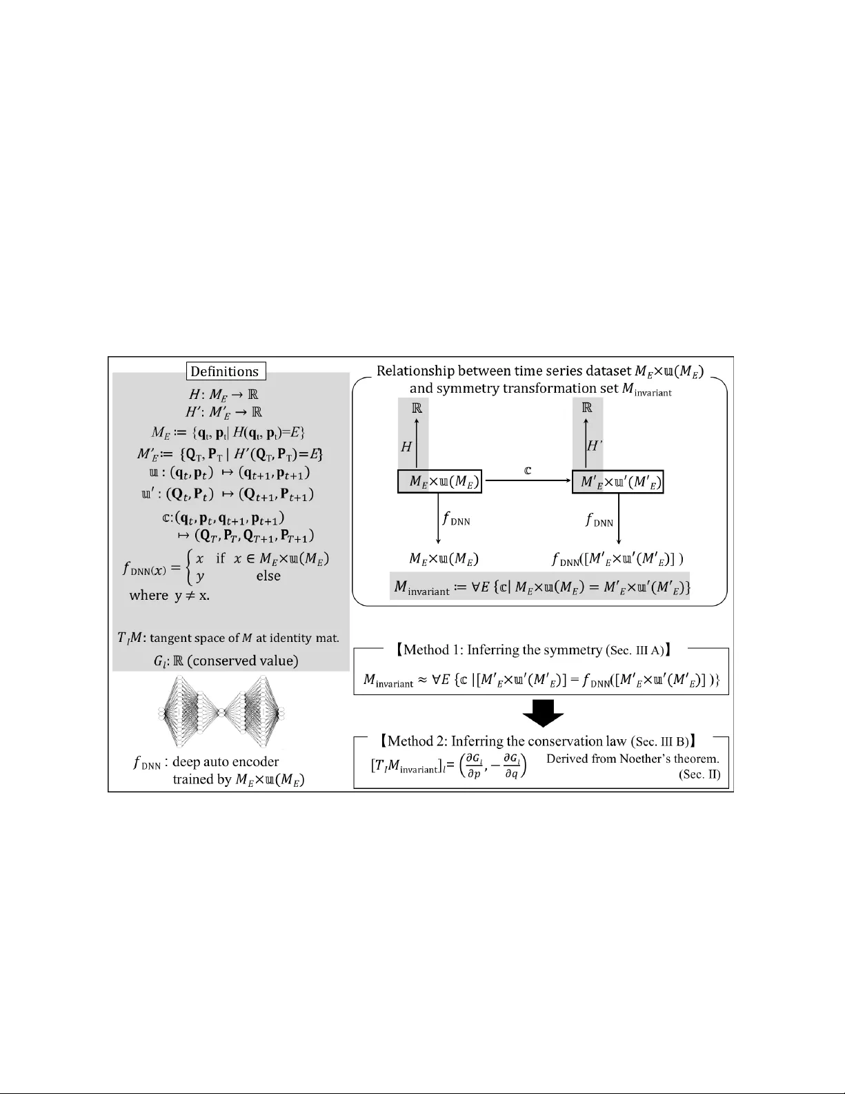
APS / 123-QED Interpr etable Conserv ation Law Estimation by Deriving the Symmetries of Dynamics fr om T rained Deep Neural Networks Y oh-ichi Mototake ∗ The Institute of Statistical Mathematics, T achikawa, T okyo 190-8562, Japan (Dated: April 21, 2020) Abstract Understanding complex systems with their reduced model is one of the central roles in scientific activi- ties. Although physics has greatly been dev eloped with the physical insights of physicists, it is sometimes challenging to b uild a reduced model of such comple x systems on the basis of insights alone. W e propose a nov el frame work that can infer the hidden conservation laws of a complex system from deep neural networks (DNNs) that ha ve been trained with ph ysical data of the system. The purpose of the proposed framework is not to analyze physical data with deep learning, but to e xtract interpretable physical information from trained DNNs. W ith Noether’ s theorem and by an e ffi cient sampling method, the proposed frame work in- fers conservation laws by extracting symmetries of dynamics from trained DNNs. The proposed framew ork is de veloped by deri ving the relationship between a manifold structure of time-series dataset and the neces- sary conditions for Noether’ s theorem. The feasibility of the proposed framework has been v erified in some primiti ve cases for which the conserv ation law is well known. W e also apply the proposed framework to conserv ation law estimation for a more practical case that is a large-scale collectiv e motion system in the metastable state, and we obtain a result consistent with that of a pre vious study . 1 I. INTR ODUCTION Understanding comple x systems with their reduced models is one of the central roles in sci- entific acti vities. Some complex systems are modeled as low-dimensional canonical dynamical systems. For e xample, reduced models have been de veloped for large-scale collecti ve motion sys- tems, which are a type of large-scale comple x system with order (e.g., plasma, acoustic wav es, or vortex systems) [1 – 5]. T o develop reduced models, collectiv e coordinates, such as the Fourier basis of a density or charge distribution [1 – 4], or a vorte x feature space [5], have been introduced. Then, a Hamiltonian that describes the coarse-grained properties of a dynamical system has been deri ved. Thus, to dev elop a reduced model, it is necessary to introduce collectiv e coordinates and deri ve the Hamiltonian in the coordinates. The obtained Hamiltonian is verified by confirming that it can reconstruct the properties of the phenomena analyzed. This approach relies heavily on the physical insights of physicists; it would not work to model a dynamical system that features a more complicated structure. One example is the collectiv e motion of living things such as fish or birds; such systems frequently hav e stable b ut very complicated patterns in a metastable state [6, 7]. The problem we consider here is how to infer the reduced model using machine learning meth- ods. As mentioned above, this in v olves the solution of two problems: estimation of a coordinate system and construction of a reduced model in the coordinate system. One way to solve these prob- lems is to construct a Hamiltonian based on a gi ven coordinate system and search for a coordinate system that improves the model. Se veral machine learning methods for inferring the Hamiltonian from a time-series dataset hav e been dev eloped [8 – 11]. These methods can be broadly di vided into two types. In one type, the Hamiltonian is inferred by regressing the data with an explicit function, such as the linear sum of multiple basis functions [8]. Howe ver , in the case of inferring a reduced model that consists of complicated unkno wn basis functions, the method only infers the approximated reduced model using an approximated function, such as a polynomial function. In the second type, a Hamiltonian is modeled by a deep learning technique [9 – 11]. In this case, an explicit function used in the first one is not required. On the basis of these machine learning methods, the search for the coordinate system could be performed using statistical criteria such as the prediction or generalization error of the inferred Hamiltonian. There are inherent di ffi culties in building a reduced model using the machine learning approach. Such an approach finds a Hamiltonian that has properties that only hold for the gi ven data. His- torically , physicists ha ve achie ved great success in constructing reduced models by abstracting 2 kno wledge obtained from observational data and building univ ersal models that can explain var - ious physical phenomena, not just the gi ven data. For example, in thermodynamics, a reduced model that describes the molecular motion of a gas was linked to chemical reaction theory by Gibbs [12, 13]. This is one of the most successful uses of a reduced model. That is, a good re- duced model and a good coordinate system mean that the performance is high not only for the gi ven data. T o reach such a successful reduced model, it is important to interpret the knowledge obtained during data analysis and dev elop a model that can be applied to di ff erent phenomena by combining the explicit and implicit kno wledge of physics. In general, an inferred Hamiltonian modeled by deep neural networks (DNNs) is hardly interpretable, because DNNs are models with enormous degrees of freedom. If all physical kno wledge is quantified, it will be possible to construct a reduced model with a DNN, b ut this is an impractical assumption at present. Therefore, it is di ffi cult by a machine learning approach to realize the same function as a physicist, who can flexibly interpret phenomena by utilizing explicit or implicit physical kno wledge and construct a reduced model. T o ov ercome this problem, we attempt to extract abstract information directly from physical data without constructing a reduced model. A coordinate system can be selected on the basis of the information. Furthermore, the obtained information can also help physicists construct a reduced model. The purpose of this study is to dev elop a machine learning framework that extracts interpretable abstract information from physical data and assist physicists in b uilding reduced models. The proposed method is developed using knowledge about DNNs. Results of several stud- ies [14 – 19] suggest that DNNs can model the distribution of datasets as manifolds, which can be embedded in a lo w-dimensional Euclidean space. Studies applying DNNs to physical data hav e employed a time-series dataset from the phase space (comprising position and momentum) [20– 24] or a spin system dataset from the configuration space [25 – 33]. In such datasets, the manifold structure, which implies that the system has a small degree of freedom, can be constructed by considering certain physical constraints, such as a conservation law . That is, a manifold structure modeled by a DNN can represent the conserv ation law or order of the system. The proposed method is deri ved from Noether’ s theorem [34], which connects the symmetry of the Hamiltonian and the conservation la w . W e deriv e the relationship between the symmetry of the Hamiltonian system and the distribution of the time-series dataset of a dynamical system. On 3 this basis, we dev elop a method of inferring the symmetry of a data manifold modeled by a deep autoencoder [15] and determine conservation laws of the system. T o infer the conserv ation laws, we only need the tangent space of the manifold of the continuous transformation group that cor- responds to the symmetry of the system. Therefore, unlike Hamiltonian estimation, conservation law estimation only requires manifold modeling with at most first-order accuracy . This means that the conserv ation law can be inferred with arbitrary precision by polynomial approximation. This paper is organized as follo ws. In Sec. II A, we sho w the deri vation of the relation- ship between the symmetry of the time-series dataset distribution and the conservation law using Noether’ s theorem. In Sec. III A, we describe our proposed method of inferring the symmetry of the time-series data manifold. In Sec. III B, we also describe another proposed method of inferring the conserv ation law from the obtained symmetry . In Sec. IV, to confirm the e ff ecti veness of the proposed methods, we apply them to three cases, one T(1) and two SO(2) systems, correspond- ing to constant-velocity linear motion, a central force system, and a large-scale collective motion system called the Reynolds model [35]. In Sec. V, we present a summary and discussion. II. THEOR Y A. Noether’ s theorem Noether’ s theorem connects continuous symmetries of a Hamiltonian system with conserv ation laws [34]. It is often described in the (2 d + 1)-dimensional extended phase space Γ × R , ( q , p ) B ( q 0 = t , q 1 , · · · , q d , p 1 , · · · , p d ) . The theorem can also be described in the (2 d + 2)-dimensional space Γ × R × R , ( q 0 = t , q 1 , · · · , q d , p 0 = − H , p 1 , · · · , p d ) . In this study , we describe the theory in the (2 d + 2)-dimensional space as follows. W e consider Hamiltonian systems in the (2 d + 2)- dimensional space Γ × R × R , and restrict ourselves to the case where the system’ s Hamiltonian belongs to a C 2 class function H ( q , p ). The Hamiltonian representation of Noether’ s theorem is described as follo ws [36]. Assume that H ( q , p ) and the canonical equations of motion ∂ H ( q , p ) ∂ q i = − ˙ p i and ∂ H ( q , p ) ∂ p i = ˙ q i are in v ariant under the infinitesimal transformation ( q 0 i , p 0 i ) = ( q i + δ q i j , p i + δ p i j ), where i = 1 , . . . , d , and j is the index of the direction of the infinitesimal transformation corresponding to a conserv ation law . Then, on the basis of Noether’ s theorem, the conserved v alue G j satisfies the follo wing equation: ( δ q i j , δ p i j ) = ∂ G j ∂ p i , − ∂ G j ∂ q i ! . (1) 4 The canonical transformation that makes the Hamiltonian system in variant is gi ven as c in v ( θ ) : Γ × R × R − → Γ × R × R , (2) ( q , p ) 7− → ( Q , P ) B ( Q ( q , p , θ ) , P ( q , p , θ ) ) , (3) where Q ( q , p , θ ) and P ( q , p , θ ) represent the inv ariant transformation functions of coordinate ( q , p ) to ( Q , P ), and θ represents a d θ -dimensional continuous parameter characterizing transformation that satisfies Q  q , p , θ = ~ 0  = q , and P  q , p , θ = ~ 0  = p . W e call this transformation an in v ariant transformation in this paper . A set of the in variant transformations characterized by the continuous parameters θ forms a Lie group. By the first-order T aylor expansion of Q i ( q , p , θ ) and P i ( q , p , θ ) around θ = ~ 0, we hav e the infinitesimal transformation ( δ q i j , δ p i j ) = ε ∂ Q i ( q , p , θ ) ∂θ j       θ = ~ 0 , ε ∂ P i ( q , p , θ ) ∂θ j       θ = ~ 0 ! , (4) where | ε |  1. Note that the dimension of continuous parameter d θ corresponds to the number of conservation laws, and with our proposed methods, we estimate conserv ation la ws including d θ . B. In variance of Hamiltonian and time-series dataset W e show the relationship between such an in variant transformation and the time-series dataset of a dynamical system in the (2 d + 2)-dimensional space ( q , p ). Here, we define the N sample time-series dataset D as D B n q i t i , p i t i , q i t i +∆ t , p i t i +∆ t o N i = 1 , where q i t i and p i t i represent the generalized position and momentum at time t i , and t i + ∆ t represents a time ev olution of ∆ t . The transformation of the (2 d + 2)-dimensional space ( q , p ) is defined as c : Γ × R × R − → Γ × R × R , (5) ( q , p ) 7− → ( Q , P ) B (Q ( q , p ) , P ( q , p ) ) , (6) where Q ( q , p ) and P ( q , p ) represent transformations functions of coordinate ( q , p ) to ( Q , P ); the transformation is not limited to the in v ariant transformation. It is assumed that c has the in verse transformation c − 1 : Γ × R × R − → Γ × R × R , (7) ( Q , P ) 7− → ( q , p ) B ( q ( Q , P ) , p ( Q , P ) ) . (8) 5 The transformed Hamiltonian H 0 ( q , p ) obeying this transformation is defined as H 0 ( Q , P ) B H ( q ( Q , P ) , p ( Q , P ) ) . The necessary and su ffi cient condition for the transformation c acting on H ( q , p ) to be identical, H 0 ( q , p ) ≡ H ( q , p ), is equiv alent to ∀ E , { q , p | H ( q , p ) = E } = { Q , P | H ( q , p ) = E } . (9) This condition is deriv ed in Appendix A and implies that the transformation inv ariance of a Hamil- tonian is equi v alent to that of the ener gy surface at each ener gy le vel in the space Γ × R × R . If the time-series dataset D has all possible data points under the Hamiltonian H ( q , p ), the subset of D with respect to q i t i and p i t i is understood as this energy surf ace. C. In variance of canonical equations and time-series dataset Next, we consider the relationship between the in variance of canonical equations of motion and the time-series dataset of the dynamical system. If the canonical equations of motion are discretized with respect to time di ff erentiation, the discretized canonical equations of motion are obtained as q t +∆ t = u ( q t , p t ) B ∂ H ( q t , p t ) ∂ p t ∆ t + q t , (10) p t +∆ t = v ( q t , p t ) B − ∂ H ( q t , p t ) ∂ q t ∆ t + p t , (11) where q t and p t represent the variables that ev olved according to time t , and u ( q t , p t ) and v ( q t , p t ) are elements of the C 1 map u defined as u : Γ × R × R − → Γ × R × R , (12) ( q t , p t ) 7− → ( q t +∆ t , p t +∆ t ) B ( u ( q t , p t ) , v ( q t , p t )) . (13) Follo wing the transformations Q ( q , p ) and P ( q , p ) in Eq. (5), these equations can be rewritten as Q T +∆ T = Q ( q t +∆ t , p t +∆ t ) = u ’ ( Q T , P T ) B Q  u  q ( Q T , P T ) , p ( Q T , P T )  , v  q ( Q T , P T ) , p ( Q T , P T )  , (14) P T +∆ T = P ( q t +∆ t , p t +∆ t ) = v ’ ( Q T , P T ) B P  u  q ( Q T , P T ) , p ( Q T , P T )  , v  q ( Q T , P T ) , p ( Q T , P T )  , (15) 6 where T = Q 0 , ∆ T = ∆ Q 0 . For the transformation ( Q , P ) = ( Q ( q , p ) , P ( q , p ) ) to be a canonical transformation, the follo wing conditions must be satisfied: u ’ ( Q T , P T ) ≡ ∂ H 0 ( Q T , P T ) ∂ P T ∆ T + Q T , (16) v ’ ( Q T , P T ) ≡ − ∂ H 0 ( Q T , P T ) ∂ Q T ∆ T + P T . (17) If H and H 0 are identically equal, the conditions of Eqs. (16) and (17) are equi valent to u ’ ( q t , p t ) ≡ u ( q t , p t ) , v ’ ( q t , p t ) ≡ v ( q t , p t ) . (18) Eq. (18) is equi valent to the follo wing condition (see Appendix B):  q t +∆ t , p t +∆ t , q t , p t | ( q t +∆ t , p t +∆ t ) =  u ( q t , p t ) , v ( q t , p t )  =  Q T +∆ T , P T +∆ T , Q T , P T | ( q t +∆ t , p t +∆ t ) =  u ( q t , p t ) , v ( q t , p t )  . (19) The time-series dataset D is understood as the part of the subspace giv en on the left side of Eq. (19). D. Noether’ s theorem and time-series dataset By combining the conditions obtained in the previous two subsections, we obtain the condition that the Hamiltonian and canonical equations are simultaneously in variant under the transforma- tion. The condition is acquired as ∀ E , ( q t +∆ t , p t +∆ t , q t , p t       H ( q t , p t ) = E , p t +∆ t = p t − ∂ H ( q t , p t ) ∂ q t , q t +∆ t = q t + ∂ H ( q t , p t ) ∂ p t ) = ( Q T +∆ T , P T +∆ T , Q T , P T       H ( q t , p t ) = E , p t +∆ t = p t − ∂ H ( q t , p t ) ∂ q t , q t +∆ t = q t + ∂ H ( q t , p t ) ∂ p t ) . (20) If the time-series dataset D has all possible data points under the Hamiltonian H ( q , p ) and the canonical equations, D is equiv alent to the subspace defined on the left side of Eq. (20). Thus, the symmetry of the Hamilton system is associated with the symmetry of the time series dataset D . The transformation set satisfying Eq. (20),  Q ( q , p ) , P ( q , p )    satisfy Eq . (20)  , is the same as the in v ariant transformation set c in v : n Q ( q , p , θ ) , P ( q , p , θ )    θ ∈ R d θ o under the discretized equations of motion. The transformed dataset in Eq. (20), ( Q T +∆ T , P T +∆ T , Q T , P T       H ( q t , p t ) = E , p t +∆ t = p t − ∂ H ( q t , p t ) ∂ q t , q t +∆ t = q t + ∂ H ( q t , p t ) ∂ p t ) , (21) 7 is obtained by the time e volution t → T of time-series dataset at t : ( Q t +∆ t , P t +∆ t , Q t , P t       H ( q t , p t ) = E , p t +∆ t = p t − ∂ H ( q t , p t ) ∂ q t , q t +∆ t = q t + ∂ H ( q t , p t ) ∂ p t ) . (22) If the Hamiltonian is giv en, we can obtain the time-ev olved dataset by e volving the dataset obeying the canonical equations of motion. Even if the Hamiltonian is not giv en, we can obtain a time- e volv ed dataset as follows. Assume that we hav e time-series dataset at ( t , t + ∆ t , t + 2 ∆ t , . . . , t + s ∆ t , . . . ), where s is Z ≥ 0 . The time transformation of data from t to T can be approximated by replacing T with T 0 : T 0 = t + s ∆ t , (23) s = arg min s | T − ( t + s ∆ t ) | . (24) There is no guarantee that all ener gy states in the reduced Hamiltonian are realized in the original complex system. In particular , when constructing a reduced model of a metastable state, only its ener gy state is realized. T o ov ercome this di ffi culty , we introduce the di ff erent e xpressions of the condition in Eq. (20). Let E i be a real number representing one energy state. W e also define the transformation c i : Γ × R × R − → Γ × R × R , (25) ( q , p ) 7− → ( Q , P ) B (Q i ( q , p ) , P i ( q , p ) ) , (26) which satisfy ( q t +∆ t , p t +∆ t , q t , p t       H ( q t , p t ) = E i , p t +∆ t = p t − ∂ H ( q t , p t ) ∂ q t , q t +∆ t = q t + ∂ H ( q t , p t ) ∂ p t ) = ( Q T +∆ T , P T +∆ T , Q T , P T       H ( q t , p t ) = E i , p t +∆ t = p t − ∂ H ( q t , p t ) ∂ q t , q t +∆ t = q t + ∂ H ( q t , p t ) ∂ p t ) . (27) Because the in variant transformation that satisfies Eq. (9) does not change the energy , the condition Eq. (20) can be re-expressed as a union of the divided conditions:  Q ( q , p ) , P ( q , p )    satisfy Eq . (20)  = T i  Q i ( q , p ) , P i ( q , p )    satisfy Eq . (27)  . This implies that the in variant transformation set for a cer- tain energy E i must include some in v ariant transformations for the total energy . Thus, candidate transformations that make the Hamiltonian and canonical equations in v ariant are obtained as the transformations that make the subspace S i B ( q t +∆ t , p t +∆ t , q t , p t       H ( q t , p t ) = E i , p t +∆ t = p t − ∂ H ( q t , p t ) ∂ q t , q t +∆ t = q t + ∂ H ( q t , p t ) ∂ p t ) (28) 8 in v ariant. This expression is useful to find the candidates of symmetries in a complex dynamical system, such as dynamics at the metastable state. In a finite time measurement or simulation, only data D of a subset of S i can be obtained. On the basis of the following two physical principles, we can estimate S i from data D . The first principle is described as follows. The subspace S i can be represented as a product space of two subspaces: S i = S a i × S b i , (29) S a i = ( q t , p t       H ( q t , p t ) = E i , p t +∆ t = p t − ∂ H ( q t , p t ) ∂ q t , q t +∆ t = q t + ∂ H ( q t , p t ) ∂ p t ) (30) =  q t , p t    H ( q t , p t ) = E i  , (31) S b i = ( q t +∆ t , p t +∆ t       H ( q t , p t ) = E i , p t +∆ t = p t − ∂ H ( q t , p t ) ∂ q t , q t +∆ t = q t + ∂ H ( q t , p t ) ∂ p t ) . (32) (33) Since the Hamiltonian is a C 2 class function, S a i is a di ff erentiable manifold. The canonical equa- tion of motion is a C 1 map because the Hamiltonian is a C 2 class function. The subspace S b i is a subspace mapped from manifold S a i according to the canonical equations of motion. Therefore, the subspace S b i is also a di ff erentiable manifold, and S i is the product of di ff erentiable manifolds S a i and S b i . From a property of product manifold, S i is understood as a di ff erentiable manifold. In- terpolation of di ff erentiable manifolds can be realized by machine learning methods such as deep learning. In our proposed framew ork, S i is estimated from a finite number of data D using a deep learning technique. The second principle is described as follows. In a canonical dynamical system in which the energy changes with time, it is not e ffi cient to acquire the data of S i because S i is a subspace of specific energy . The important cases of a comple x dynamical system to be modeled as a reduced model are at the stable or metastable state. Also, one of the final goals of this study is to extract the conserv ation la ws in a large-scale collectiv e motion system at a metastable state. In the stable or metastable state, the energy of the system is conserved: H ( q t , p t ) = H ( q t +∆ t , p t +∆ t ) = E . Therefore, for the purpose of this study , e ffi cient data acquisition is realized. In this study , we only deal with classical systems. A similar relationship holds between the data manifold and the symmetry of the system in canonical quantum field theory . In the canonical quantum field theory , the Hamiltonian is gi ven as H ( φ ( x ) , π ( x ) , x ) , (34) 9 where φ ( x ) is the field, π ( x ) is the canonical momentum conjugate of φ ( x ), and x = ( ct , x 1 , x 2 , x 3 ) is the Minko wski space; φ ( x ) and π ( x ) satisfy the commutation relation [ φ ( x ) , π ( y ) ] = i δ (4) ( x − y ) (35) [ φ ( x ) , φ ( y ) ] = [ π ( x ) , π ( y ) ] = 0 . (36) The infinitesimal transformation is gi ven as Φ i ( X ) = φ i ( x ) + δφ i ( x ) , (37) Π i ( X ) = π i ( x ) + δπ i ( x ) , (38) X i = x i + δ x i . (39) Similar to the nested relations between coordinates and time in the classical system, the canonical quantum field theory states that a field and its conjugate momentum hav e a nested Minko wski space. Therefore, as in the discussion for classical systems, the follo wing relation is giv en as a condition of the in v ariant transformation of a Hamiltonian system: ∀ E , { φ t +∆ t , π t +∆ t , φ t , π t | H ( φ t , π t ) = E , ( φ t +∆ t , π t +∆ t ) = u ( φ t , π t ) } = { Φ T +∆ T , Π T +∆ T , Φ T , Π T | H ( φ t , π t ) = E , ( φ t +∆ t , π t +∆ t ) = u ( φ t , π t ) } , where u is an equation of motion such as the KleinGordon equation of a scalar particle. E. DNN and data manif old As mentioned in Sec. II D, the subspace S i could be modeled as a di ff erentiable manifold using machine learning models. Some well-trained DNNs ha ve the ability to model the distrib ution of a training dataset as a di ff erentiable manifold [14 – 19]. In this paper , we refer to such a di ff erentiable manifold as a data manifold. W e explain how a DNN models a d m -dimensional manifold in d in -dimensional space x us- ing one of the simplest DNNs: a feed forward three-layer DNN, for which the input has d in dimensions, the hidden layer has d h ( > d in ) dimensions, and the output has d out ( < d in ) = d m di- mensions. The mapping function f DNN ( x ) =  f 1 ( x ) , f 2 ( x ) , · · · , f d out ( x )  of the DNN is defined as f DNN ( x ) = w h h = w h ϕ ( w in x ), where h = ( h 1 , h 2 , · · · , h d h ) is the d h -dimensional output of the hid- den layer . W e define ϕ ( · ) as ϕ ( w in x ) = ( ϕ 1 , ϕ 2 , · · · , ϕ d h ) , ϕ j = ϕ h P d in i  w in i j x i i , where ϕ is the acti vation function. Usually , a sigmoid or ReLU function is used as the acti v ation function. These 10 FIG. 1. Schematic diagram of the mapping structure of a two-dimensional input space in a DNN trained with data distributed on a black curve. The arrows indicate the compression direction of the input space in the mapping from the input to the hidden layer . acti vation functions are constructed using linear and flat domains. On the basis of these properties of activ ation functions, ϕ j maps the input subspace related to the linear domain of the acti vation function to a one-dimensional space to align the vector ( w 0 j , w 1 j · · · , w d in j ). If the number of ϕ j sharing the same input subspace is d out , the ϕ j defines a d out -dimensional sub-hyperplane. The DNN models the data distribution by continuously pasting these sub-hyperplanes as if they were the tangent spaces of a data manifold. That is, the DNN embeds the input space in the output space by pasting the sub-hyperplanes and compresses the tangent direction of these sub-hyperplanes (Fig. 1). Deeper and more complex DNNs can be understood as a collection of such three-layer DNN. Thus, such deeper DNNs can model more complex manifold structures as a combination of simple manifold structures modeled by a three-layer DNN [17]. Note that the output of a three- layer DNN, a part of the deeper DNN, is referred to as a hidden layer . This is only one example of ho w a DNN models a data manifold. Ho we ver , many studies hav e suggested that there are resemble property in successful trained DNNs [14 – 19]. By replacing the input space from x to Γ × R × R , we can also model a time-series data manifold S i using DNN. In this study , using a trained DNN that models a time-series data manifold S i , we propose a method of extracting information about the symmetry of a dynamical system. As described later in Sec. V, our proposed frame work does not require special DNNs, so we can directly utilize the v ast kno wledge obtained from studies on physical data analysis using DNNs. This is why we select the DNN from multiple machine learning models that can be used to model manifolds. 11 III. METHOD In this section, we describe our proposed framework for estimating the conservation law from a time-series dataset of dynamics. The schematic diagram of the proposed frame work is sho wn in Fig. 2. The framew ork consists of two methods. In Sec. III A, on the basis of the deri vation of the relationship between the symmetry of the time-series dataset distribution and the conservation law (Sec. II), we propose a method of inferring the symmetry of data manifold using the Monte Carlo sampling method. In Sec. III B, we describe the proposed method of inferring the conserv ation law from the obtained symmetry . FIG. 2. Schematic diagram of the proposed framew ork. A. Method 1: Inferring the symmetry of data manifold using Monte Carlo sampling method In this subsection, we propose a general method of inferring the symmetric property of data manifolds, which is not limited to the physical time-series dataset. It can be inferred from the 12 FIG. 3. Schematic diagram of method of extracting in variant transformation using autoencoder . discussion in Sec. II E that data points that are not on the manifold in the input space are attracted to the manifold (Fig. 1). Once the data points are attracted to the manifold in the hidden layer , they continue to exist on the manifold in the output f ( x ). W e propose a method based on this property of DNNs for extracting the symmetry of the data manifold using a deep autoencoder [15]. The deep autoencoder is a model that compresses the input space to a lo w-dimensional hidden layer and decompresses the layer to an output space with the same dimension as the input space. In the decompression process, only the subspace of the input space around the data manifold is recov ered because of the DNN property . On the basis of this property , we can ev aluate whether a transformation X ( · ) causes the dataset distribution { x i } N i = 1 to remain in the same subspace of the data manifold (Fig. 3). The procedure is as follows. First, we train the deep autoencoder using { x i } N i = 1 as a training dataset. Second, we input the transformed dataset { X ( x i ) } N i = 1 into the trained deep autoencoder . Note that the deep autoencoder is not trained on the transformed dataset. Third, we e v aluate the transformation X ( · ) using the mean squared error between the input distrib ution of the dataset and its mapped distribution: E samp [ X ( · )] = 1 N N X i = 1  X ( x i ) − f DNN [ X ( x i )]  2 . (40) A smaller E samp v alue implies that X ( · ) is a more in variant transformation. Using the criterion E samp , we approximate the in v ariant transformation set as ( X ( · )       arg min X E samp [ X ( · )] ) . (41) 13 T o infer the conservation law , it is necessary to estimate the in v ariant transformation set M in variant of the manifold S i . The in v ariant transformation set M in variant is defined as M in variant B n Q S i ( · , · , θ ) , P S i ( · , · , θ )    θ o . (42) In Eq. (40), by substituting { x i } N i = 1 for D = n q i t i , p i t i , q i t i +∆ t , p i t i +∆ t o N i = 1 and X ( · ) for the transformation c : ( Q ( · , · ) , P ( · , · ) ) , we can approximate M in variant as M in variant ∼ ( Q ( · , · ) , P ( · , · )       arg min Q ( · , · ) , P ( · , · ) E samp  Q ( · , · ) , P ( · , · )  ) , (43) where dataset D is generated from dynamics data at energy E i . The approximated in v ariant trans- formation set is obtained approximately by sampling from the probabilistic density: P ( Q ( · , · ) , P ( · , · ) ) ∼ 1 Z exp  − N 2 σ 2 E samp  Q ( · , · ) , P ( · , · )   , (44) where σ is set as small as necessary and Z is a normalization constant. Note that to actually perform this sampling, it is necessary to first gi ve a concrete coordinate system of ( q i , p i ) in which physicists want to search conserv ation la ws. As mentioned in Sec. II A, continuous symmetries form a Lie group. Using the continuous parameter set θ = { θ k } d θ k = 1 , we define the representation of the Lie group as a 2 d × 2 d -dimensional matrix A i j ( θ ) = a i j ( θ ), where 2 d is the degree of freedom of the target Hamiltonian system. θ is a continuous parameter set, and A ( 0 ) = I . In the follo wing, candidate in variant transformations are searched for within the Lie group representations. The inv ariant transformation is obtained by sampling an element a jk of the matrix A following the probability distrib ution P( a 11 , a 12 , a 21 , · · · , a 2 d 2 d ) = 1 Z exp  − N 2 σ 2 E samp ( a 11 , a 12 , a 21 , · · · , a 2 d 2 d )  . (45) T o perform this sampling, we need to specify σ . Ideally , σ should be set to 0. Howe v er , it is necessary to set σ to an appropriate finite value because errors are included in the time-series dataset and the training results of DNN. Such σ a ff ected by noise cannot be set in adv ance. In addition, the target distributions in this study are assumed to be the global flat minima, because the same E samp surface follo wing the in variant transformation e xists. Generally , such a target distribution needs an enormous amount of time to sample. Therefore, in this study , we use the replica-exchange Monte Carlo (REMC) method [37] as a sampling method to overcome these problems. Such a method enables us to perform e ffi cient sampling by parallel sampling with 14 di ff erent noise intensities of σ while e xchanging noise intensities with each other . In the state of a large noise, we can realize global sampling from the abstract distrib ution P 0 ( a 11 , a 12 , a 21 , · · · , a 2 d 2 d ) = 1 Z 0 exp  − N 2 σ 0 2 E samp ( a 11 , a 12 , a 21 , · · · , a 2 d 2 d )  , (46) where σ 0 > σ . By exchanging this sampling information with the state of a small noise, we can perform e ffi cient sampling from the target distrib ution P ( a 11 , a 12 , a 21 , · · · , a 2 d 2 d ). The detailed ex- planation of REMC method and the setting parameters of the method are described in Appendix E, and the target σ is determined by analyzing the sampling results as described in Appendix F. The procedure of Method 1 is summarized in Algorithm 1. Note that there is no description of how to train a DNN in this study . In the training of the deep autoencoder , the number of nodes in the hidden layer is an important hyperparameter . On the other hand, since this is a quantity that determines how much the phenomenon is to be reduced, it is considered to be provided by the physicist. Algorithm 1 Estimation of the in variant transformation set Input : dataset D = n q i t i , p i t i , q i t i +∆ t , p i t i +∆ t o N i = 1 in a gi ven coordinate system. Output : In variant transformation set D a = { ( a 11 , a 12 · · · , a 1 d , a 21 · · · , a 2 d 2 d ) n a } N a n a = 1 . Step 1 : T rain the deep autoencoder with dataset D . Step 2 : Using the trained deep autoencoder and REMC method, sampling transformation parameters a 11 , a 12 , a 21 , · · · , a 2 d 2 d from multiple probability distributions P 0 ( a 11 , a 12 , a 21 , · · · , a 2 d 2 d ) corresponding to di ff erent noise intensities σ 0 . Step 3 : Select σ 0 from the distribution structure of the sampling results and output the sampling result of the selected σ 0 state as D a . B. Method 2: Inferring the conservation law from obtained symmetry From the N a sampling results D a B { ( a 11 , a 12 · · · , a 1 d , a 21 · · · , a 2 d 2 d ) n a } N a n a = 1 in Sec. III A, we propose a method of estimating the infinitesimal transformation, which represents the in v ariance of the Hamiltonian and the equation of motion. The set of in variant transformation M in variant is characterized by the d θ -dimensional continuous parameter θ . Therefore, M in variant is a d θ -dimensional di ff erential manifold. Note that M in variant 15 forms a Lie group as we mentioned in Sec. II A. The infinitesimal transformation is estimated as the tangent vector of M in variant at θ = 0 . Using A ( θ ), we estimate M in variant as M in variant ∼          A ( θ )          q p                  θ ∈ R d θ          . (47) By serializing the transformation matrix A ( θ ), we define the vector A 0 ( θ ) = ( a 0 1 ( θ ) , · · · , a 0 d 0 ( θ )) B ( a 11 ( θ ) , · · · , a 1 d ( θ ) , a 21 ( θ ) , · · · , a 2 d ( θ ) , · · · , a d 1 ( θ ) , · · · , a 2 d 2 d ( θ )) , (48) where d 0 = 4 d 2 . The implicit function representation of the manifold M in variant is defined as                      f 1 ( a 0 1 , · · · , a 0 d 0 ) = 0 . . . f d 0 − d θ ( a 0 1 , · · · , a 0 d 0 ) = 0 . (49) In the representation of the implicit function, the infinitesimal transformation is estimated as the tangent vector of the manifold M in variant at the position e I = ( · · · , a i j = 0 , · · · , a i i = 1 , · · · ) , (50) where i , j and e I is the representation of the identity matrix I in the A 0 ( θ ) space. W e estimate this tangent space T I M in variant = T e I M in variant from the sampling results D a obtained in Sec. III A. The Jacobian matrix of f k for parameters of the subset A 0 , ( b 1 , b 2 , · · · , b d θ ) ⊂ A 0 , is defined as J kl = ∂ f k ( a 0 1 , ··· , a 0 d 0 ) ∂ b l . If the Jacobian matrix at A 0 = e I becomes nonsingular , from the implicit function theorem, v ariables other than ( b 1 , b 2 , · · · , b d θ ), { c k } d 0 − d θ k = 1 B A 0 \ { b l } d θ l = 1 , can be expressed as c k = g i ( b 1 , · · · , b d θ ). This implies that, around e I , the implicit equations in Eq. (49) representing the manifold M in variant can be decomposed into the follo wing d 0 − d θ simultaneous equations:                      h 1 ( c 1 , b 1 , · · · , b d θ ) = 0 . . . h d 0 − d θ ( c d 0 − d θ , b 1 , · · · , b d θ ) = 0 , (51) where b l corresponds to the continuous parameter θ l of the continuous transformation  Q ( q , p , θ ) , P ( q , p , θ )  . Di ff erentiating these equations with respect to b l around a point e I yields d 0 − d θ simultaneous par - 16 tial di ff erential equations,                      ∂ ∂ b l h 1 ( c 1 , b 1 , · · · , b d θ ) | A 0 = e I = 0 . . . ∂ ∂ b l h d 0 − d θ ( c d 0 − d θ , b 1 , · · · , b d θ ) | A 0 = e I = 0 . (52) Solving these simultaneous partial di ff erential equations giv es the tangent vector A 0 ( b l ) ∂ b l     A 0 = e I of the manifold around e I . Using the tangent vector as the nonserialized representation A ( b l ) ∂ b l     A = I , we can estimate an infinitesimal transformation as          δ q l δ p l          = ε A ( b l ) ∂ b l      A = I          q p          = ε                  ∂ a 1 1 ∂ b l | A = I · · · ∂ a 2 d 1 ∂ b l | A = I . . . . . . . . . ∂ a 1 2 d ∂ b l | A = I · · · ∂ a 2 d 2 d ∂ b l | A = I                           q p          . (53) Thus, the in v ariant transformation is obtained as the tangent vector of the manifold M in variant at point e I . Therefore, if c k can be regressed around e I as the first-order polynomial of { b l } d θ l = 1 , the conservation law can be inferred without approximation. Compared with the Hamiltonian estimation and conservation law estimation, this is the adv antage of conservation law estimation, because, in general, the Hamiltonian estimation requires infinite-order polynomial approximation. On the other hand, the estimation accuracy of the tangent space T e I M in variant from finite data with noise is often lo w . In this study , we propose a method of estimating the infinitesimal transform with high accurac y by using all sampled transformation data, not only data around e I . Another way to a void this problem is also discussed in Sec. V. The simultaneous equations in Eq. (51) can be estimated by the following procedure. First, the upper limit of the dimension of the manifold M in variant is estimated by applying principal compo- nent analysis and the elbo w” method to D a as described in [38]. Alternativ ely , the approximate dimension of M in variant can be estimated by using the manifold dimension estimation method such as the method described in [39]. Using such an estimated dimension of M in variant , we can prepare candidate dimension d 0 θ . Second, we extract one variable set ( b 1 , b 2 , · · · , b d 0 θ ). By orthogonal dis- tance regression [40], we regress D b ≡ { ( c k , b 1 , b 2 , · · · , b d 0 θ ) n a } N a n a = 1 to a d b -order implicit polynomial function, ˆ h k ( c k , b 1 , b 2 , · · · , b d 0 θ ; β, γ , d 0 θ ) B d b X s 0 = 0 d b X s 1 = 0 · · · d b X s d 0 θ = 0 γ s 0 s 1 s 2 ··· s d 0 θ β s 0 s 1 s 2 ··· s d 0 θ c s 0 k b s 1 1 b s 2 2 · · · b s d 0 θ d 0 θ = 0 , (54) 17 where β is the regression coe ffi cient, and γ is a binary v ector indicating whether the basis is se- lected. The indicator vector γ and the dimension of the manifold d 0 θ are determined by a model selection method, such as the Bayesian information criterion (BIC) [41]. T o select the model, it is necessary to estimate the likelihood. The method of estimating the likelihood is described in Appendix G. If d θ ≤ 2, d 0 θ can be determined by visualization. Note that, unlike the estimation of the tangent space T e I M in variant , the upper limit d b of the order of polynomial function must be suf- ficiently large because the entire sampling data is regressed. This regression and model selection is performed for all c k ; then, an implicit function representation of M in variant can be obtained. From the obtained simultaneous equations, we obtain the simultaneous di ff erential equations. If the Jacobian matrix J kl is singular , the solution of the simultaneous equations di v erges or becomes indefinite. In that case, the variable set { ( b 1 , · · · , b d 0 θ ) } is extracted again and the same procedure is repeated. If the Jacobian matrix J kl is nonsingular , we can obtain the infinitesimal transforma- tion according to Eq. (53). In this method, by narro wing down the regressing area of D a to the neighborhood of e I , we obtain a higher accurate estimation of infinitesimal transformation with a lo wer-order polynomial function in Eq. (54). Algorithm 2 Estimation of infinitesimal transformation Input : Sampling results of Method 1, D a = { ( a 11 , a 12 · · · , a 1 d , a 21 · · · , a 2 d 2 d ) n a } N a n a = 1 , and d 0 θ . Output : Infinitesimal transformation, δ q l , δ p l . Step 1 : Extract D b = { ( c k , b 1 , b 2 , · · · , b d 0 θ ) n a } N a n a = 1 from D a . Step 2 : Fit D b with the implicit polynomial function ˆ h k ( c k , b l 1 , b l 2 , · · · , b l d 0 θ ; β, γ, d 0 θ ) [Eq. (54)] for each c k . Step 3 : Estimate the likelihood [Eq. (G1)] by numerical integration of Z [Eq. (G2)]. Step 4 : Select the indicator v ector γ and the dimension d 0 θ of M in variant in Eq. (54) for each c k using the BIC, . Step 5 : Determine whether the Jacobi matrix J kl = ∂ h k ( c k , b 1 , ··· , b d θ ) ∂ b l is nonsingular . If J kl is singular , return to Step 1 and re-extract D 0 b . Step 6 : Di ff erentiate the obtained simultaneous equations with respect to b l around a point e I to obtain Eq. (52). Step 7 : Solve the simultaneous equations in Eq. (52) and obtain the infinitesimal transformation, δ q l , δ p l . 18 IV . RESUL TS W e ev aluate the proposed method using one geometrical structure and three physical systems: (i) a half sphere, (ii) constant-velocity linear motion, (iii) a two-dimensional central force system, and (iv) a collectiv e motion system. Case (i) has a rotational symmetry . In case (i), we confirm that Method 1 can obtain a set of transformations corresponding to the symmetry . Cases (ii) and (iii) are systems that conserve the momentum and angular momentum, respectiv ely . Using these cases, we verified Method 2. Finally , we apply both proposed methods to (i v), which is a complicated collecti ve motion system, and attempted to infer the collecti ve coordinate and conservation law . In each case, the parameters of DNN are set as described in Appendix H, and REMC are set as described in Appendix E. (i) Half sphere The dataset of case (i) was generated by the function x 2 1 + x 2 2 + x 2 3 = r , ( x 3 > 0) , (55) where r was set to be 0 . 25. W e generated 1,671 samples according to Eq. (55). The dataset of case (i) [sho wn in Fig. 4(a)] was used to v erify the ability of Method 1 described in Sec. III A, which extracts the symmetry . W e set the coordinate system as ( x 1 , x 2 , x 3 ) and limit the transforma- tion on the x 1 - x 2 plane. In such a case, the transformation matrix A is defined as A =                  a 11 a 21 0 a 12 a 22 0 0 0 0                  . (56) In this coordinate system, the half sphere has a rotation symmetry and a mirror symmetry . The rotation symmetry transformation is represented as A rot ( θ rot ) =          cos( θ rot ) sin( θ rot ) − sin( θ rot ) cos( θ rot )          , (57) where θ rot is a rotation angle, and the mirror symmetry transformation is represented as A mirror ( θ mirror ) =          cos(2 θ mirror ) sin(2 θ mirror ) sin(2 θ mirror ) − cos(2 θ mirror )          , (58) 19 where θ mirror is an angle of the mirror plane with the x 1 axis. The mirror symmetry is a discrete sym- metry; therefore, the in v ariant transformation of the half sphere is represented as A tot ( θ rot , θ mirror ) B A rot ( θ rot )[ A mirror ( θ mirror )] m , where m B { 0 , 1 } and A rot ( θ rot )[ A mirror ( θ mirror )] 0 B A rot ( θ rot ) , (59) A rot ( θ rot )[ A mirror ( θ mirror )] 1 B          cos(2 θ mirror − θ rot ) sin(2 θ mirror − θ rot ) sin(2 θ mirror − θ rot ) − cos(2 θ mirror − θ rot )          = A mirror  θ 0  , (60) θ 0 B θ mirror − θ rot 2 . (61) By comparing Eq. (56) with Eqs. (59) and (60), we obtain the implicit function representation of the in v ariant transformation A tot ( θ rot , θ mirror ) as                                                  a 2 11 + a 2 21 = 1 a 2 11 + a 2 12 = 1 ( a 11 + a 22 )( a 11 − a 22 ) = a 2 11 − a 2 22 = 0 ( a 21 − a 12 )( a 21 + a 12 ) = a 2 21 − a 2 12 = 0 a 2 21 + a 2 22 = 1 a 2 12 + a 2 22 = 1 . (62) Method 1 was applied to such a system. The sampling results of a i j are sho wn in Fig. 4(b) as black dots. In the figures, the red curves were fitted by the selected implicit polynomial functions using the BIC. The fitting results are                                                  a 2 11 + 0 . 99 a 2 21 = 1 a 2 11 + a 2 12 = 1 a 2 11 − a 2 22 = 0 a 2 21 − a 2 12 = 0 a 2 21 + a 2 22 = 1 a 2 12 + a 2 22 = 1 , (63) where we determine d 0 θ to be 1 by visualizing the distribution of D a . 20 FIG. 4. Results of case (i): half sphere. (a) Dataset using the ev aluation. There are 1,671 samples. (b) Black dots represent sampling distributions obtained by Method 1 and red curves represent fitting curves estimated by Method 2. Each graph shows six combinations of four transformation v ariables a i j . (ii) Constant-velocity linear motion The dataset of case (ii) was generated using the one-dimensional Hamiltonian system H 2 = p 2 2 m , (64) where m was set to be 1. W e generated 1,000 samples by solving Eq. (64). In this case, we show that the proposed method can infer the momentum conservation law . W e set the coordinate system as ( q , 1 , p , 1). In such a coordinate system, q and p are related as p = m ˙ q . This means that q and p hav e the same coordinate transformation. Thus, the transformation matrix A is defined as A =                         a b 0 0 0 1 0 0 0 0 a 0 0 0 0 1                         . (65) As a result, two parameters a and b must be sampled. The sampling results of a i j are shown in Fig. 5 as black dots and the red curves were fitted by the selected implicit polynomial function using the BIC. The fitting result is a = 1 . 0 . (66) 21 FIG. 5. Results of case (ii): constant-v elocity linear motion. (a) Conceptual diagram of constant-velocity linear motion. (b) Black dots represent sampling distribution obtained by Method 1 and the red line repre- sents the fitting curve estimated by Method 2. The simultaneous partial di ff erential equations in Eq. (52), where b l = b , were obtained from the fitting results. From the solution of the simultaneous partial di ff erential equations, we obtained the infinitesimal transformation            δ q =  ∂ a ∂ b q +  ∂ b ∂ b =  δ p =  ∂ a ∂ b p = 0 , (67) where we determined d 0 θ to be 1 by visualizing the distribution of D a . By substituting this Eq. (67) into Eq. (1) and solving the equations, we estimated the conserved value G δ as G δ = 1 . 0 ε p . This result sho ws that the momentum p was conserv ed. (iii) T wo-dimensional central for ce system The dataset of case (iii) was generated using the Hamiltonian system H 3 = 1 2 m p 2 + G m M | q | , (68) where q B ( q 1 , q 2 ), p B ( p 1 , p 2 ), and m , M , and G were set to be 1. W e generated 1,000 samples by solving Eq. (68). W e set the coordinate system as ( q 1 , q 2 , p 1 , p 2 ). In such a coordinate system, 22 q j and p j are related as p j = m ˙ q j . Thus, q j and p j hav e the same coordinate transformation, and the transformation matrix A is defined as A =                         a 11 a 21 0 0 a 12 a 22 0 0 0 0 a 11 a 21 0 0 a 12 a 22                         . (69) As a result, only four parameters a i j must be sampled. In the canonical dynamics of H 3 , it is impossible to transform one orbit to another with the same energy but di ff erent long-axis radii using the linear transformation A in Eq. (69). Therefore, the in v ariant transformation for S i can be represented as a product of in v ariant transformation for sub- space S radii i for specific energy and long-axis radii. This implies that the in variant transformation set for certain energy E i and certain long-axis radii must include some in variant transformations for S i . On the basis of this property of the Hamilton system of H 3 , we apply the proposed method only to the time-series dataset of a circular orbit with radius 1. The sampling results of a i j are shown in Fig. 6 as black dots and the red curve in each figure was fitted by the selected polynomial function using the BIC. The fitting results are                                                  a 2 11 + 0 . 99 a 2 21 = 1 a 2 11 + 0 . 98 a 2 12 = 1 a 11 − a 22 = 0 a 21 + 0 . 99 a 12 = 0 a 2 21 + 1 . 01 a 2 22 = 1 . 01 a 2 12 + 1 . 02 a 2 22 = 1 . 02 , (70) where we determine d 0 θ to be 1 by visualizing the distribution of D a . The simultaneous partial di ff erential equations in Eq. (52), where b l = a 21 , were obtained from the fitting results. By solving 23 FIG. 6. Results of case (iii): two-dimensional central force system. (a) Conceptual diagram of two- dimensional central force system. (b) Black dots represent sampling distributions obtained by Method 1 and red curv es represent fitting curves estimated by Method 2. Each graph shows six combinations of four transformation v ariables a i j . the simultaneous partial di ff erential equations, we obtained the infinitesimal transformation δ q = ε          ∂ a 11 ∂ a 21 ∂ a 21 ∂ a 21 ∂ a 12 ∂ a 21 ∂ a 21 ∂ a 21          q = ε           − 2 × 0 . 99 a 21 2 a 11     A = I 1 − 1 / 0 . 99 − 2 a 21 1 . 01 × 2 a 22     A = I           q (71) =          0 ε − 1 . 01 ε 0          q ≈          0 ε − ε 0          q , (72) δ p = ε          ∂ a 11 ∂ a 21 ∂ a 21 ∂ a 21 ∂ a 12 ∂ a 21 ∂ a 21 ∂ a 21          p ≈          0 ε − ε 0          p , (73) where the values in the final formula are to one decimal place. By substituting Eqs. (72) and (73) into Eq. (1) and solving the equation, we estimated the conserv ed v alue G δ as G δ = ε ( x 1 p 2 − x 2 p 1 ). This result sho ws that the angular momentum was conserved. (iv) Collective motion system In this case, we apply our frame work to an N R -body collectiv e motion system called the Reynolds boid model [35]. In this model, each indi vidual mov es following three forces, which 24 are the force attracting each other , separating each other , and aligning the orientation of each other: d p j d t = − W att p j − P k ∈ K att p k n att ! + W sep          X k ∈ K sep ( q j − q k ) | q j − q k |          + W ali q j − P k ∈ K ali q k n ali ! , (74) d q j d t = p j , (75) K att = ( k       | q k − q j | < r att , arccos p k · p j | p k || p j | ! < θ att , k , j ) , K sep = ( k       | q k − q j | < r sep , arccos p k · p j | p k || p j | ! < θ sep , k , j ) , K ali = ( k       | q k − q j | < r ali , arccos p k · p j | p k || p j | ! < θ ali , k , j ) , n att = X k ∈ K att 1 , n ali = X k ∈ K ali 1 , where q B ( q 1 , q 2 , q 3 ), p B ( p 1 , p 2 , p 3 ), and j , k represent the index of an individual. The at- traction, separation, and alignment terms are represented by the first, second, and third terms in Eq. (74), and each force has the interaction range, r att , r sep , r ali , and angle of vie w , θ att , θ sep , θ ali , respecti vely . The parameters W att , W sep , W ali , r att , r sep , r ali , θ att , θ sep , and θ ali of the Reynolds boid model can be tuned to simulate the collecti v e motion of li ving things such as birds or fish [35, 42]. In this study , we focused on a parameter set that simulates the torus-type behavior of a school of fish in the sea. Such a torus-type collectiv e motion can be realized in a two-dimensional space. Therefore, we set the dimension to two in this study . By solving Eq. (74), we generated 2,000 steps of time-series data of the torus-type collecti ve motion by 200 indi viduals. T o infer the conserv ation law of collecti ve motion, we need to set a candidate collecti ve co- ordinate. In this study , we set the collecti ve coordinate on the basis of the following consider- ations. First, from the visual symmetry of the motion, the av erage position ( ¯ q 1 , ¯ q 2 ) and av erage momentum ( ¯ p 1 , ¯ p 2 ) of all particles over time are set as the origin of the coordinate system. Sec- ond, since the same behavior is observed regardless of the individual, each indi vidual is consid- ered to hav e no degree of freedom. From these considerations, we set the coordinate system as ( ˜ q , ˜ p ) = ( q 1 − ¯ q 1 , q 2 − ¯ q 2 , p 1 − ¯ p 1 , p 2 − ¯ p 2 ), and prepared the dataset as D = { ˜ q ( t i ) i , ˜ p ( t i ) i , ˜ q ( t i + ∆ t ) i , ˜ p ( t i + ∆ t ) i } N R T i = 1 (76) B { ˜ q ( t jk ) jk , ˜ p ( t jk ) jk , ˜ q ( t jk + ∆ t ) jk , ˜ p ( t jk + ∆ t ) jk } h j , k i , (77) 25 where N R = 200, T = 2 , 000, and h j , k i represents all combinations of individuals j and time steps k . W e randomly selected 5,000 samples from this dataset for the training of DNN. Then, the transformation matrix A is defined as A =                         a 11 a 21 0 0 a 12 a 22 0 0 0 0 a 11 a 21 0 0 a 12 a 22                         . (78) The sampling results of a i j are shown in Fig. 7(b) as black dots and the red curves fitted by the selected implicit polynomial functions using the BIC. The fitting results of the selected implicit polynomial functions are                                                  a 2 11 + 1 . 03 a 2 21 + 0 . 039 a 11 a 21 = 1 a 2 11 + 1 . 18 a 2 12 + 0 . 077 a 11 a 12 = 1 a 11 − 1 . 016 a 22 + 0 . 016 a 2 11 = 0 a 21 + 1 . 077 a 12 = 0 − 0 . 038 a 22 + a 2 21 + 1 . 005 a 2 22 + 0 . 051 a 21 a 22 = 0 . 967 − 0 . 031 a 22 + a 2 12 + 0 . 877 a 2 22 + 0 . 056 a 12 a 22 = 0 . 845 , (79) where we determine d 0 θ = 1 by visualizing the distribution of D a . The simultaneous partial di ff er- ential equations in Eq. (7), where b l = a 12 , were obtained from the fitting results. By solving the simultaneous equations, we obtained the infinitesimal transformation δ q = ε          ∂ a 11 ∂ a 21 ∂ a 21 ∂ a 21 ∂ a 12 ∂ a 21 ∂ a 21 ∂ a 21          q = ε           − 1 . 03 × 2 a 21 − 0 . 039 a 11 2 a 11 + 0 . 039     A = I 1 − 1 / 1 . 077 − 2 a 21 − 0 . 051 a 22 1 . 005 × 2 a 22 − 0 . 038 + 0 . 051 a 12     A = I           q (80) =          0 . 019 ε ε − 0 . 928 ε 0 . 026 ε          q ≈          0 ε − ε 0          q , (81) δ p = ε          ∂ a 11 ∂ a 21 ∂ a 21 ∂ a 21 ∂ a 12 ∂ a 21 ∂ a 21 ∂ a 21          p ≈          0 ε − ε 0          p , (82) where the values in the final formula are to one decimal place. By substituting Eqs. (81) and (82) into Eq. (1) and solving the equation, the conserved v alue G δ was estimated as G δ = ε ( x 1 p 2 − x 2 p 1 ). This result sho ws that the angular momentum was conserved. 26 FIG. 7. Results of case (iv): collecti ve motion system. (a) Simulation snapshot of torus-type collective motion. The simulation data were applied to the proposed method. (b) Black dots represent sampling distributions obtained by Method 1 and red curves represent fitting curves estimated by Method 2. Each graph sho ws six combinations of four transformation variables a i j . V . SUMMAR Y AND DISCUSSION From the results of case (i), we confirm that Method 1 could be used to extract the symmetry . The results of cases (ii) and (iii), wherein the e xpected conserv ation laws were inferred, sho w that Method 2 is e ff ecti ve. By comparing cases (i) and (iii), we observe di ff erences in the selected implicit polynomial functions in the a 11 - a 22 and a 21 - a 12 spaces. These di ff erences emerged from the mirror symmetry in case (i). This finding supports the assertion that the method works well in extracting the symmetry of a system. For a more practical collecti ve motion system [i.e., case (iv)], we inferred the angular momentum conserv ation la w; the results thereof are consistent with a pre vious study [42]. In the pre vious study , it is suggested that angular momentum is conserv ed in torus-type swarming patterns. Additionally , the finding of a conserv ation law in the collectiv e coordinates, where the degree of freedom of an individual was degenerated and the origin of the coordinates is the av erage position and momentum of the swarm, suggests that a dynamical system with a large de gree of freedom can be reduced to a central force dynamical system. The present study deals only with the case of a single conservation law . If there are multiple 27 conserv ation laws, the dimension of the manifold D a becomes increase. In such a case, Eq. (52) has multiple orthogonal solutions. Theoretically , the proposed method can still handle such a problem, but the number of combinations of polynomial regressions [Eq. (54)] increases exponentially , and the Jacobian matrix is more lik ely to be singular . Therefore, it is necessary to dev elop a more e ffi cient method of estimating an infinitesimal transformation. T o estimate an infinitesimal transformation, one needs only to estimate a tangent space around the identity element. As there is a finite sample, in the proposed method, the manifold formed by Lie groups is re gressed over the entire space. It is expected that the tangent space can be directly estimated by orthogonal basis decomposition by introducing v arious constraints. In this study , we used the deep autoencoder to model the time-series data manifolds; nonethe- less, there is no need to use the deep autoencoder . The only requirement for a machine learning model is that it has a mapping function that can determine whether it is on or outside the manifold. From this perspecti ve, the deep autoencoder can be replaced with another type of DNN model, such as a variational autoencoder [43] or a generativ e adv ersarial network [44]. Additionally , a feed-forward-type DNN, which is widely used in DNN research, can be used in our proposed method by additionally training a neural network that reconstructs the input data from the out- put layer of the feed forward neural network. The same method should be feasible for use with machine learning models that hav e mapping functions that embed data manifolds into the output space (e.g., the kernel method). Thus, the proposed frame work can potentially extract interpretable physical knowledge from the wide range of machine learning models. Note that the structure of the extracted manifold changes depending on the DNN model and its training settings. This is because the reduced model acquired inside the DNN changes depending on the DNN model and the training settings. Ho w to learn time-series dataset using a certain DNN model and training settings are understood as the implicit construction of the reduced model. In this study , we showed that the proposed framew ork can infer the hidden conservation laws of a complex system from DNNs that have been trained with physical data of the system. On the basis of the obtained results, it is expected that the knowledge of physical data embedded in the trained DNNs in pre vious studies and the knowledge of physicists can be merged. This should accelerate the research on the construction of reduced models. 28 A CKNO WLEDGMENTS I w ould like to thank Dr . Y . Ando, Professor S. Goto, Dr . S. T akabe, Professor H. Hino, Professor K. Fukumizu, Professor K. Hukushima, Professor T . Ikeg ami, Professor K. Ishika wa, Mr . H. Y amashita, Professor Y . Y ue, and Mr . K. Sakamoto for useful discussions. This work was supported by KAKENHI grant numbers JP17H01793 and JP19K12111. A ppendix A: Derivation of equivalent condition to make Hamiltonian in variant The identity condition H ( q , p ) ≡ H 0 ( q , p ) has the equiv alent e xpression ∀ ( q , p ) , H ( q , p ) = H 0 ( q , p ) . (A1) This condition can be transformed to an equi valent conditional e xpression represented by a set, ∀ E , { q , p | H ( q , p ) = E } = { q , p | H 0 ( q , p ) = E } , (A2) which is proved in Appendix C. Replacing q , p with the transformed parameters Q , P does not change the set: { q , p | H 0 ( q , p ) = E } = { Q , P | H 0 ( Q , P ) = E } . Therefore, Eq. (A2) is re written as ∀ E , { q , p | H ( q , p ) = E } = { Q , P | H 0 ( Q , P ) = E } . (A3) From the definition of the transformed Hamiltonian H 0 , H 0 ( Q , P ) B H ( q ( Q , P ) , p ( Q , P ) ) = H ( q , p ) are satisfied. By substituting these into Eq. (A3), we obtain the target condition equiv alent to the identity condition H ( q , p ) ≡ H 0 ( q , p ) as ∀ E , { q , p | H ( q , p ) = E } = { Q , P | H ( q , p ) = E } . (A4) A ppendix B: Derivation of equivalent condition to make canonical equations in variant The identity condition in Eq. (18), u ( q t , p t ) ≡ u 0 ( q t , p t ) ∧ v ( q t , p t ) ≡ v 0 ( q t , p t ) , (B1) has the equi valent e xpression ∀ ( q t , p t ) , ( u ( q t , p t ) , v ( q t , p t )) = ( u 0 ( q t , p t ) , v 0 ( q t , p t )) . (B2) 29 This condition can be transformed to the following equiv alent conditional expression represented by a set: ∀ ( q t +∆ t , p t +∆ t ) , { q t , p t | ( q t +∆ t , p t +∆ t ) = ( u ( q t , p t ) , v ( q t , p t )) } = { q t , p t | ( q t +∆ t , p t +∆ t ) = ( u ’ ( q t , p t ) , v ’ ( q t , p t )) } . (B3) The proof of the equiv alence of Eqs. (B2) and (B3) is a multiv ariable case of the proof described in Appendix C. By treating q t +∆ t , p t +∆ t as a set of elements, we transform the condition in Eq. (B3) to the equi valent condition (see the proof in Appendix D) { q t +∆ t , p t +∆ t , q t , p t | ( q t +∆ t , p t +∆ t ) = ( u ( q t , p t ) , v ( q t , p t )) } = { q t +∆ t , p t +∆ t , q t , p t | ( q t +∆ t , p t +∆ t ) = ( u ’ ( q t , p t ) , v ’ ( q t , p t )) } . (B4) Replacing q t , p t , q t +∆ t , p t +∆ t with the transformed parameters Q T , P T , Q T +∆ T , P T +∆ T does not change the set: { q t +∆ t , p t +∆ t , q t , p t | ( q t +∆ t , p t +∆ t ) = ( u ’ ( q t , p t ) , v ’ ( q t , p t )) } (B5) = { Q T +∆ T , P T +∆ T , Q T , P T | ( Q T +∆ T , P T +∆ T ) = ( u ’ ( Q T , P T ) , v ’ ( Q T , P T )) } . (B6) Therefore, Eq. (B4) is re written as { q t +∆ t , p t +∆ t , q t , p t | ( q t +∆ t , p t +∆ t ) = ( u ( q t , p t ) , v ( q t , p t )) } = { Q T +∆ T , P T +∆ T , Q T , P T | ( Q T +∆ T , P T +∆ T ) = ( u ’ ( Q T , P T ) , v ’ ( Q T , P T )) } . (B7) From the definition of the transformed canonical equations [Eqs. (14) and (15)], we obtain  Q T +∆ T , P T +∆ T  =  u ’ ( Q T , P T ) , v ’ ( Q T , P T )  (B8) ⇔  q t +∆ t , p t +∆ t  =  u ( q t , p t ) , v ( q t , p t )  . (B9) By substituting this into Eq. (B7), we obtain the target condition equi valent to the identity condi- tion in Eq. (18) as { q t +∆ t , p t +∆ t , q t , p t | ( q t +∆ t , p t +∆ t ) = ( u ( q t , p t ) , v ( q t , p t )) } = { Q T +∆ T , P T +∆ T , Q T , P T | ( q t +∆ t , p t +∆ t ) = ( u ( q t , p t ) , v ( q t , p t )) } . (B10) 30 A ppendix C: Proof of Eq. (A1) ⇔ Eq. (A2) and Eq. (B2) ⇔ Eq. (B3) The problem can be abstracted as the proposition belo w: ∀ x , f ( x ) = g ( x ) ⇔ ∀ E , { x | f ( x ) = E } = { x | g ( x ) = E } , (C1) where f ( x ) and g ( x ) are single-v alued functions. • Proof of ∀ x , f ( x ) = g ( x ) → ∀ E , { x | f ( x ) = E } = { x | g ( x ) = E } (C2) The contrapositi ve of (C2) is ∃ E , { x | f ( x ) = E } , { x | g ( x ) = E } → ∃ x , f ( x ) , g ( x ). This contra- positi ve is pro ved as follo ws. Since ∃ E , { x | f ( x ) = E } , { x | g ( x ) = E } , there exists E 0 and x 0 , which satisfy f ( x 0 ) = E 0 , but g ( x 0 ) , E 0 . Therefore, ∃ x , f ( x ) , g ( x ) is satisfied because f ( x 0 ) , g ( x 0 ).  • Proof of ∀ E , { x | f ( x ) = E } = { x | g ( x ) = E } → ∀ x , f ( x ) = g ( x ) (C3) The contrapositi ve of (C3) is ∃ x , f ( x ) , g ( x ) → ∃ E , { x | f ( x ) = E } , { x | g ( x ) = E } . This contrapos- iti ve is prov ed as follows. Select one x 0 from x , which satisfies f ( x 0 ) , g ( x 0 ) and f ( x 0 ) = E 0 . Since f ( x ) is a single-v alued function, x 0 is not included in the set of x that satisfies g ( x ) = E 0 . Thus, { x | f ( x ) = E 0 } , { x | g ( x ) = E 0 } holds. Therefore, ∃ E , { x | f ( x ) = E } , { x | g ( x ) = E } is satisfied.  A ppendix D: Proof of Eq. (B3) ⇔ Eq. (B4) The problem can be abstracted as the proposition belo w: ∀ b , { x | f ( x ) = b } = { x | g ( x ) = b } ⇔ { x , b | f ( x ) = b } = { x , b | g ( x ) = b } , (D1) where f ( x ) and g ( x ) are single-v alued functions. • Proof of ∀ b , { x | f ( x ) = b } = { x | g ( x ) = b } → { x , b | f ( x ) = b } = { x , b | g ( x ) = b } (D2) 31 The contrapositi ve of (D2) is { x , b | f ( x ) = b } , { x , b | g ( x ) = b } → ∃ b , { x | f ( x ) = b } , { x | g ( x ) = b } . This contrapositiv e is proved as follows. Since { x , b | f ( x ) = b } , { x , b | g ( x ) = b } , there is a set of x 0 and b 0 , which satisfies f ( x 0 ) = b 0 and g ( x 0 ) , b 0 . Therefore, { x | f ( x ) = b 0 } , { x | g ( x ) = b 0 } holds. It means that ∃ b , { x | f ( x ) = b } , { x | g ( x ) = b } is satisfied.  • Proof of { x , b | f ( x ) = b } = { x , b | g ( x ) = b } → ∀ b , { x | f ( x ) = b } = { x | g ( x ) = b } (D3) The contrapositi ve of (D3) is ∃ b , { x | f ( x ) = b } , { x | g ( x ) = b } → { x , b | f ( x ) = b } , { x , b | g ( x ) = b } . This contrapositiv e is prov ed as follo ws. Since ∃ b , { x | f ( x ) = b } , { x | g ( x ) = b } , there is a set of b 0 and x 0 , which satisfies f ( x 0 ) = b 0 and g ( x 0 ) , b 0 . Therefore, { x , b | f ( x ) = b } , { x , b | g ( x ) = b } is satisfied.  A ppendix E: Replica exchange Monte Carlo (REMC) method and its parameters Using A 0 B ( a 11 , a 12 , a 21 , · · · , a 2 d 2 d ), we re-express Eq. (45) as P( A 0 ) = 1 Z exp  − N 2 σ 2 E samp ( A 0 )  . (E1) The REMC method takes samples from the joint density P( A 0 1 , · · · , A 0 l , · · · , A 0 L ) = L Y l = 1 1 Z exp " − N 2 σ 2 l E samp ( A 0 ) # , (E2) where σ l > σ l + 1 and σ L = σ . In the REMC method, sampling from the joint density P( A 0 1 , · · · , A 0 l , · · · , A 0 L ) is performed on the basis of the follo wing updates. 1 Sampling from each density P( A 0 1 , · · · , A 0 l , · · · , A 0 L ) Sampling A 0 l from P( A 0 l ) B 1 Z l exp  − N 2 σ 2 l E samp ( A 0 l )  , where Z 0 is the normalization constant. The sampling is performed by a con ventional Monte Carlo method, such as the Metropo- lis–Hastings algorithm [45]. 32 2 Exchange between two densities corresponding to noise intensity σ The exchanges between the configurations A 0 l and A 0 l + 1 correspond to adjacent in verse tem- peratures follo wing the probability R = min(1 , r ), where r = P( A 0 1 , · · · , A 0 l + 1 , A 0 l , · · · , A 0 L ) P( A 0 1 , · · · , A 0 l , A 0 l + 1 , · · · , A 0 L ) = P( A 0 l + 1 )P( A 0 l ) P( A 0 l )P( A 0 l + 1 ) = exp  N 2 [ σ − 2 l + 1 − σ − 2 l ][ E ( A 0 l + 1 ) − E samp ( A 0 l )]  . Sampling from a distribution with a larger σ l tends not to have a local minimum. Hence, sampling from the joint density P( A 0 1 , A 0 2 · · · A 0 L ) o vercomes the local minima in distrib utions with small σ l and enables the rapid con v ergence of sampling. In the execution of EMC sampling, we adopted the Metropolis–Hastings algorithm [45] to sample each state of σ l . When we performed the Metropolis–Hastings sampling, a candidate for the next sample a l next i j is picked from the conditional probability distrib ution with precondition a l previous i j P( a l next i j | a l previous i j ) = 1 2 U l ( − U l ≤ a l next i j ≤ U l ) , (E3) where U l is set as U l =          C ( e N σ − 2 l ≥ 1) C ( eN σ − 2 l ) d ( e N σ − 2 l < 1) . (E4) C , d , and e in Eq. (E4) are set as T able I for the e valuation of the proposed method in Sec. IV. In case (ii) constant-velocity linear-motion, the sampling parameters C of a and b in Eq. (65) were set as di ff erent v alues [The values are described as ( C of a ) / ( C of b ) in the column of (ii) constant- velocity of T able I]. Each state of σ l was determined follo wing the exponential function [46]: σ − 2 l =          0 . 0 ( l = 1) σ − 2 min γ ( l − 1) − L ( l , 1) , (E5) where σ min is set as root-mean-square error (RMSE) for A = I in trained DNN, because it repre- sents the minimum v alue of E samp . L and γ are set as shown in T able I for each case. 33 T ABLE I. Parameters of REMC method. Parameter name (i) Half sphere (ii) Constant-velocity (iii) Central force (iv) Collecti ve motion Sampling size N a 10,000 10,000 10,000 10,000 L 20 30 30 30 γ 1.4 1.9 1.4 1.4 C 3.0 0.03 / 0.3 0.3 0.3 d 0.6 0.7 0.8 0.8 e 5.0 1.0 5.0 5.0 σ min 4.42 × 10 − 2 5.41 × 10 − 5 1.67 × 10 − 1 8.0 Burn-in length 1.000 10,000 1,000 10,000 Selected noise intensity σ noise 8.66 × 10 − 2 5.41 × 10 − 5 3.45 71.3 A ppendix F: Noise intensity of sampling Depending on the di ff erence in σ noise , the sampling results corresponding to lo w MSE and the sampling results corresponding to high MSE are obtained [Fig. 8(a)]. In the lo w-MSE region, the transformation matrix corresponding to the identity matrix is sampled [Fig. 8(b)]. In the high- MSE region, the transformation matrix corresponding to the rotation matrix is sampled [Fig. 8(d)]. At intermediate noise intensities, sampling between both conditions is achiev ed [Fig. 8(c)]. On the basis of such a structure, in this research, we select the noise intensity σ noise that realizes the non-identity transformation such as σ noise = 3 . 452 of Fig. 8. For the e v aluation of the proposed method in Sec. IV, we select the noise intensity σ noise for each e v aluation case as sho wn in T able I. 34 FIG. 8. Qualitativ e transition of sampling results due to the increase in noise intensity . The figures describe the qualitati ve transition of case (iii) central force system where rotation symmetry exists. (a) Distributions of MSE with di ff erent noise intensities. (b), (c), and (d) Sampling results of a 11 and a 21 at each noise intensity . A ppendix G: Estimation of likelihood for the model selection Under the assumption that N a samples of transformation are gi ven with Gaussian noise, the follo wing likelihood is defined for a statistical selection of implicit function. P  ~ b 1 , ~ b 2 , · · · , ~ b N a  = 1 Z exp        − 1 2 σ 2 b N a X n a = 1 D h ~ b n a , f ( c k , b 1 , b 2 , · · · , b d 0 θ ; β, γ , d 0 θ ) i 2        , (G1) Z = Z ∞ −∞ d ~ b n a exp ( − 1 2 σ 2 b D h ~ b n a , f ( c k , b 1 , b 2 , · · · , b d 0 θ ; β, γ , d 0 θ ) i 2 ) , (G2) σ b =        1 N a N a X n a = 1 D h ~ b n a , f ( c k , b 1 , b 2 , · · · , b d 0 θ ; β, γ , d 0 θ ) i 2        1 2 , (G3) ~ b n a = ( c k , b 1 , b 2 , · · · , b d 0 θ ) n a , (G4) 35 T ABLE II. Parameters of DNN and its training. In the “Network structure”, the number of nodes is sho wn in the order from left to right: input layer – first layer – second layer – third layer – output layer . Parameter name (i) Half sphere (ii) Constant-velocity (iii) Central force (iv) Collecti v e motion T raining datasize N 1,671 1,000 1,000 5,000 Network structure 3-10-2-10-3 4-10-1-10-4 8-20-1-20-8 8-20-1-20-8 Acti vation function sigmoid tanh sigmoid sigmoid T raining algorithm Adam Adam Adam Adam T raining iteration 50,000 100,000 50,000 50,000 Minibatch size 10 30 10 10 Library theano [47, 48] scikit-learn [49] theano theano where D h ~ b n a , f ( c k , b 1 , b 2 , · · · , b d 0 θ ; β, γ , d 0 θ ) i is the minimum distance from a data point ~ b n a to a sub- space defined by the implicit function f ( c k , b 1 , b 2 , · · · , b d 0 θ ; β, γ , d 0 θ ) = 0. The normalized constant Z is estimated numerically as the Riemann sum. A ppendix H: DNN model and its training parameters In this section, we describe the DNN models and their training settings. In this study , we used deep autoencoders as DNN models. In all cases (i), (ii), (iii), and (i v), the DNNs consisted of an input layer , three hidden layers, and an output layer . The number of nodes in each layer was set as sho wn in the “Network structure” in T able II. The activ ation functions of the deep autoencoders were set as the sigmoid or h yperbolic tangent functions as sho wn in the “ Activ ation function” in T able II. The sigmoid function is defined as sigmoid( x ) = 1 1 + exp( − x ) , (H1) and the tanh function is defined as tanh( x ) = exp( x ) − exp( − x ) exp( x ) + exp( − x ) . (H2) The numbers of samples used for training DNN are sho wn in T able II as “T raining datasize N ”. The Adam method [50] was used for training. The training iterations are shown in T able II. In the 36 training, the data were divided into minibatches whose sizes are shown in T able II as “Minibatch size”. ∗ mototake@ism.ac.jp [1] S. T omonaga, Prog. Theor . Phys. 5 , 544 (1950). [2] D. Bohm and D. Pines, Phys. Re v . 82 , 625 (1951). [3] D. Pines and D. Bohm, Phys. Re v . 85 , 338 (1952). [4] S. T omonaga, Prog. Theor . Phys. 13 , 467 (1955). [5] P . G. Sa ff man, V ortex Dynamics (Cambridge Uni versity Press, Cambridge, 1992). [6] T . V icsek and A. Zafeiris, Phys. Rep. 517 , 71 (2012). [7] T . Ikegami, Y . Mototake, S. K obori, M. Oka, and Y . Hashimoto, Philosophical T ransactions of the Royal Society A: Mathematical, Physical and Engineering Sciences 375 , 20160351 (2017). [8] M. Schmidt and H. Lipson, Science 324 , 81 (2009). [9] S. Greydanus, M. Dzamba, and J. Y osinski (Curran Associates, Inc., 2019) pp. 15353–15363. [10] P . T oth, D. J. Rezende, A. Jaegle, S. Racani ` ere, A. Botev , and I. Higgins, arXi v preprint arXi v:1909.13789 (2019). [11] R. Bondesan and A. Lamacraft, arXi v preprint arXiv:1906.04645 (2019). [12] J. W . Gibbs, T ransactions of the Connecticut Academy of Arts and Sciences 3 , 108 (1875–1876). [13] J. W . Gibbs, T ransactions of the Connecticut Academy of Arts and Sciences 3 , 343 (1877–1878). [14] B. Irie and M. Kawato, T ransactions of the Institute of Electronics, Information and Communication Engineers D 73 , 1173 (1990). [15] G. E. Hinton and R. R. Salakhutdinov , Science 313 , 504 (2006). [16] P . P . Brahma, D. W u, and Y . She, IEEE Transactions on Neural Networks and Learning Systems 27 , 1997 (2016). [17] R. Basri and D. W . Jacobs, in 5th International Conference on Learning Representations, ICLR 2017, T oulon, F r ance, April 24-26, 2017, Confer ence T rack Pr oceedings (OpenRevie w .net, 2017). [18] S. Rifai, Y . N. Dauphin, P . V incent, Y . Bengio, and X. Muller , in Advances in Neural Information Pr ocessing Systems 24 , edited by J. Shawe-T aylor , R. S. Zemel, P . L. Bartlett, F . Pereira, and K. Q. W einberger (Curran Associates, Inc., 2011) pp. 2294–2302. [19] Y . Mototake and T . Ikegami, International Symposium on Artificial Life and Robotics (2015). 37 [20] K. Y eo, arXiv preprint arXi v:1710.01693 (2017). [21] J. Morton, A. Jameson, M. J. K ochenderfer , and F . W itherden, in Advances in Neural Information Pr ocessing Systems 31 , edited by S. Bengio, H. W allach, H. Larochelle, K. Grauman, N. Cesa-Bianchi, and R. Garnett (Curran Associates, Inc., 2018) pp. 9258–9268. [22] S. H. Rudy , J. N. Kutz, and S. L. Brunton, arXi v preprint arXiv:1808.02578 (2018). [23] N. T akeishi, Y . Kawahara, and T . Y airi, in Advances in Neural Information Pr ocessing Systems 30 , edited by I. Guyon, U. V . Luxbur g, S. Bengio, H. W allach, R. Fergus, S. V ishwanathan, and R. Garnett (Curran Associates, Inc., 2017) pp. 1130–1140. [24] B. Lusch, J. N. Kutz, and S. L. Brunton, Nature Communications 9 , 4950 (2018). [25] T . Ohtsuki and T . Ohtsuki, J. Phys. Soc. Jpn. 85 , 123706 (2016). [26] T . Ohtsuki and T . Ohtsuki, J. Phys. Soc. Jpn. 86 , 044708 (2017). [27] P . Broecker , J. Carrasquilla, R. G. Melko, and S. T rebst, Scientific Reports 7 , 8823 (2017). [28] K. ChNg, J. Carrasquilla, R. G. Melko, and E. Khatami, Phys. Re v . X 7 , 031038 (2017). [29] J. Carrasquilla and R. G. Melko, Nature Physics 13 , 431 (2017). [30] A. T anaka and A. T omiya, J. Phys. Soc. Jpn. 86 , 063001 (2017). [31] H. Saito and M. Kato, J. Phys. Soc. Jpn. 87 , 014001 (2017). [32] E. P . V an Nieuwenburg, Y .-H. Liu, and S. D. Huber , Nature Physics 13 , 435 (2017). [33] P . Zhang, H. Shen, and H. Zhai, Phys. Rev . Lett. 120 , 066401 (2018). [34] A. Noether , Math. Phys. KI II 235 (1918). [35] C. W . Re ynolds, in Pr oceedings of the 14th Annual Confer ence on Computer Graphics and Interactive T echniques , SIGGRAPH 87 (Association for Computing Machinery , New Y ork, NY , USA, 1987) p. 2534. [36] J. Struckmeier and C. Riedel, Annalen der Physik 11 , 15 (2002). [37] K. Hukushima and K. Nemoto, J. Phys. Soc. Jpn. 65 , 1604 (1996). [38] M. O. Ulfarsson and V . Solo, IEEE T ransactions on Signal Processing 56 , 5804 (2008). [39] E. Le vina and P . J. Bickel, in Advances in Neural Information Pr ocessing Systems 17 , edited by L. K. Saul, Y . W eiss, and L. Bottou (MIT Press, 2005) pp. 777–784. [40] P . J. Brown and W . A. Fuller , Statistical analysis of measur ement err or models and applications: Pr o- ceedings of the AMS-IMS-SIAM J oint Summer Researc h Confer ence held on J une 10-16, 1989, with support fr om the National Science F oundation and the US Army Resear ch O ffi ce , V ol. 112 (American Mathematical Soc., 1990). 38 [41] G. Schwarz, Annals of Statistics 6 , 461 (1978). [42] I. D. Couzin, J. Krause, R. James, G. D. Ruxton, and N. R. Franks, Journal of Theoretical Biology 218 , 1 (2002). [43] D. P . Kingma and M. W elling, arXi v preprint arXiv:1312.6114 (2013). [44] I. Goodfello w , J. Pouget-Abadie, M. Mirza, B. Xu, D. W arde-Farle y , S. Ozair, A. Courville, and Y . Bengio, in Advances in Neural Information Pr ocessing Systems 27 , edited by Z. Ghahramani, M. W elling, C. Cortes, N. D. Lawrence, and K. Q. W einberger (Curran Associates, Inc., 2014) pp. 2672–2680. [45] W . K. Hastings, Biometrika 57 , 97 (1970). [46] K. Nagata and S. W atanabe, Neural Networks 21 , 980 (2008). [47] F . Bastien, P . Lamblin, R. Pascanu, J. Bergstra, I. J. Goodfellow , A. Bergeron, N. Bouchard, and Y . Bengio, “Theano: ne w features and speed improv ements, ” Deep Learning and Unsupervised Fea- ture Learning NIPS 2012 W orkshop (2012). [48] J. Bergstra, O. Breuleux, F . Bastien, P . Lamblin, R. Pascanu, G. Desjardins, J. T urian, D. W arde-Farley , and Y . Bengio, in Pr oceedings of the Python for Scientific Computing Confer ence (SciPy) (2010) oral Presentation. [49] F . Pedregosa, G. V aroquaux, A. Gramfort, V . Michel, B. Thirion, O. Grisel, M. Blondel, P . Pretten- hofer , R. W eiss, V . Dubourg, J. V anderplas, A. Passos, D. Cournapeau, M. Brucher, M. Perrot, and E. Duchesnay , Journal of Machine Learning Research 12 , 2825 (2011). [50] D. P . Kingma and J. Ba, arXiv preprint arXi v:1412.6980 (2014). 39