Building HVAC Scheduling Using Reinforcement Learning via Neural Network Based Model Approximation

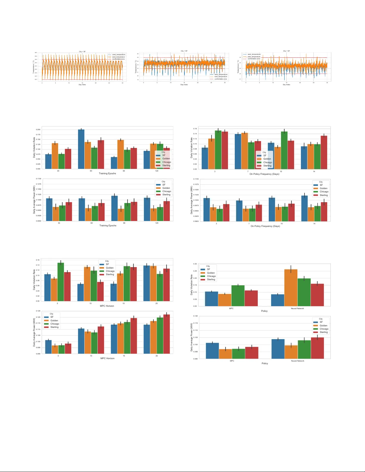
Building H V A C Scheduling Using Reinforcement Learning via Neural Network Based Model Approximation ∗ Chi Zhang Department of Computer Science University of Southern California Los Angeles, CA zhan527@usc.edu Sanmukh R. Kuppannagari Department of Electrical and Computer Engineering University of Southern California Los Angeles, CA kuppanna@usc.edu Rajgopal Kannan US Army Research Lab- W est Playa Vista, CA rajgopak@usc.edu Viktor K. Prasanna Department of Electrical and Computer Engineering University of Southern California Los Angeles, CA prasanna@usc.edu ABSTRA CT Buildings sector is one of the major consumers of energy in the United States. The buildings H V A C (Heating, V entilation, and Air Conditioning) systems, whose functionality is to maintain thermal comfort and indoor air quality (IA Q), account for almost half of the energy consumed by the buildings. Thus, intelligent scheduling of the building HV AC system has the potential for tremendous energy and cost savings while ensuring that the control objectiv es (thermal comfort, air quality) are satised. Traditionally , rule-based and model-based approaches such as linear-quadratic regulator (LQR) have be en used for sche duling HV A C. Howev er , the system comple xity of HV AC and the dy- namism in the building environment limit the accuracy , eciency and robustness of such methods. Recently , several works hav e fo- cused on model-free deep reinforcement learning based techniques such as Deep Q-Network (DQN). Such methods require extensiv e interactions with the environment. Thus, they are impractical to implement in real systems due to low sample eciency . Safety- aware exploration is another challenge in r eal systems since certain actions at particular states may result in catastrophic outcomes. T o address these issues and challenges, we propose a model- based reinforcement learning approach that learns the system dy- namics using a neural network. Then, we adopt Model Predictive Control (MPC) using the learned system dynamics to p erform con- trol with random-sampling shooting method. T o ensure safe explo- ration, we limit the actions within safe range and the maximum absolute change of actions according to prior knowledge. W e evalu- ate our ideas through simulation using widely adopted EnergyPlus ∗ This work has been sponsored by the U.S. Army Research Oce (ARO) under award number W911NF1910362 and the U .S. National Science Foundation (NSF) under award number 1911229. Permission to make digital or hard copies of all or part of this work for personal or classroom use is granted without fee provided that copies are not made or distributed for prot or commercial advantage and that copies bear this notice and the full citation on the rst page. Copyrights for components of this work owned by others than ACM must be honored. Abstracting with credit is permitted. T o copy other wise, or r epublish, to post on servers or to redistribute to lists, requires prior specic permission and /or a fee. Request permissions from permissions@acm.org. BuildSys ’19, November 13–14, 2019, New Y ork, NY, USA © 2019 Association for Computing Machinery . ACM ISBN 978-1-4503-7005-9/19/11. . . $15.00 https://doi.org/10.1145/3360322.3360861 tool on a case study consisting of a two zone data-center . Experi- ments show that the average deviation of the trajectories sampled from the learned dynamics and the ground truth is below 20% . Compared with baseline approaches, we reduce the total energy consumption by 17 . 1% ∼ 21 . 8% . Compared with model-free rein- forcement learning approach, we reduce the required numb er of training steps to converge by 10x. CCS CONCEPTS • Computing metho dologies → Reinforcement learning ; • Hardware → T emperature control . KEY W ORDS neural network dynamics, model-based reinforcement learning, hvac control, smart buildings, data center cooling, model predictiv e control A CM Reference Format: Chi Zhang, Sanmukh R. Kuppannagari, Rajgopal Kannan, and Viktor K. Prasanna. 2019. Building H V AC Scheduling Using Reinforcement Learning via Neural Network Based Model Approximation. In The 6th ACM Inter- national Conference on Systems for Energy-Ecient Buildings, Cities, and Transportation (BuildSys ’19), November 13–14, 2019, New Y ork, N Y , USA. A CM, New Y ork, N Y , USA, 10 pages. https://doi.org/10.1145/3360322.3360861 1 IN TRODUCTION The energy consumption by buildings consist of 40% of the total energy and 70% of total electricity in the United States [ 18 ]. Of the total energy consumption of buildings, the Heating, V entilation and Air-Conditioning (HV A C) system accounts for 50% while the rest is used for lighting, electrical appliances, electric vehicles, etc. The main objective of the HV A C system is to maintain the indoor temperature and air quality . An intelligent H V A C scheduling system will, additionally , save energy and cost while satisfying the objective. The HV A C system is a nonlinear system and has complex system dynamics with a large number of subsystems including chillers, boilers, heat pumps, pip es, ducts, fans, pumps and heat exchangers [ 11 ]. In this paper , we assume the combination of equipment to operate by the HV A C system is xed and focus on how to set the temperature point for local controllers to reduce the energy BuildSys ’19, November 13–14, 2019, New Y ork, NY, USA Chi Zhang et al. consumption or cost while maintaining the thermal comfort at given level. Traditional approaches for set point scheduling include PID control [ 28 ] and rule-based supervisor y controllers [ 26 ]. The PID controller is a fee dback proportional–integral–derivative controller which works by simply turning on/o the HV A C systems. Some advanced H V A C sche duling systems employ rule-based super visory controllers given historical operation experience. Such systems require no system modeling and design eort, howev er , they require an experienced and professional operator to constantly monitor and control the system which increases operational costs. Moreover , these traditional approaches are reactive in nature i.e. they are based on fe edback from the system and lack the ability to anticipate how the system evolves. This hinders their energy performance as - (i) the thermal inertia of the building leads to delayed eect of control action requiring more aggressive actions, and (ii) the inability to predict and account for e xternal disturbances such as weather , electricity price and o ccupancy conditions leads to sub- optimal decision making. Recent success of deep learning has led to the dev elopment of several deep reinforcement learning (DRL) base d approaches for HV A C scheduling [ 15 , 27 , 29 ]. These data-driven approaches learn an agent to schedule the H V A C system by interacting with the en- vironment. DRL can be generally divided into model-free approach and model-based approach. In model-free DRL, the agent learns the policy by directly interacting with the environment. The agent ex- plores the environment by extensively trial-and-error . Ho wever , for a constraine d system such as HV AC which enfor ces soft constraints of the feasible region of op eration i.e. thermal comfort b ounds, model-free DRL techniques such as Deep Q-Network [ 25 ] require a large amount of operational data (obtained via interactions) to converge (also kno wn as low sample eciency ) which is dicult to gather in a real system. Thus, the practical alternative is to adopt model-base d RL ap- proaches. The model for RL algorithm can be obtaine d by devel- oping a thermal dynamics model [ 24 ]. However , the complexity of the H V AC system and the dynamism of the building environ- ment makes it a daunting task [ 4 ]. Thus, an alternative is to use the readily available historical data on HV AC operation and learn a general function approximator ( e.g. neural network) for building system dynamics [ 16 ]. Planning algorithms such as linear-quadratic regulator (LQR) [ 3 ] can be used on the learned dynamic to perform HV AC scheduling to minimize energy consumption with thermal comfort constraints. In this paper , we develop a model-based reinforcement learning approach for smart building HV A C control by learning the system dynamics using operation data to t a neural network. Then, we perform Model Predictive Control (MPC) [ 9 ] using the learned dy- namics with random-sampling shooting method [ 19 ]. Compared with model-free approaches, our approach is able to train an accu- rate model with limited amount of data and achieve good control performance without extensive trial-and-error with the systems. Compared with manually design model, our approach is more gen- eral and applicable to various building models since it learns system dynamics automatically from data. Our main contributions ar e as follows: • W e analyze the fundamental drawbacks of previous model- free DRL-based approaches and emphasize the importance of sample data eciency in data-driven approaches. • W e propose a model-based DRL approach for building HV AC control that trains the system dynamics with neural net- works online. Our approach is both data ecient and self- adaptive online with gradually changing system dynamics (e.g. outdoor temperature). • Given trained system dynamics, we perform Mo del Pre- dictive Control (MPC) to produce action for the next step that minimizes the energy cost and the temperature con- straints violation collectively with random-sampling shoot- ing method. • T o support real-time inference, we train an auxiliary policy network that imitates the output of MPC. • W e conduct experiments on a two-room data center and show that our approach r educes the total energy consump- tion by 17 . 1% ∼ 21 . 8% . Compared with model-free reinforce- ment learning approach, we reduce the required number of training steps to converge by 10x. 2 RELA TED W ORK In [ 4 ], the author proposes to estimate the thermal load and use a regulator and a disturbance rejection comp onent to keep the room at comfort temperature. In [ 12 ], the author proposes a novel multi-input multi-output (MIMO) to model H V A C system and uses a linear-quadratic regulator (LQR) [ 3 ] to optimize control perfor- mance and to stabilize the proposed HV A C system. In general, exact modeling of HV A C system dynamics is dicult and several data-driven approaches are proposed recently . In [ 13 ], the authors propose linear models for system identication and limit each con- trol variable to a safe range informed by historical data for explo- ration. Then, the authors minimize a length- 𝐿 trajectory to obtain the control sequence, execute the action at rst step and re-run the optimization. Although they achiev e signicant performance improvement over baseline controllers, they did not consider distri- bution shift over time, which requires data aggregation and model ne-tuning. In [ 27 ] and [ 10 ], the author proposes to use De ep Q- Network [ 25 ] to control HV A C systems. In [ 15 ], the author proposes a EnergyPlus based research envir onment for developing reinforce- ment learning appr oaches for data-center HV AC contr ol. In [ 7 ], the author sho ws pr omising r esults of approximating the Model Predic- tive Controller using neural networks. In [2], the author proposes to learn system dynamics using Articial Neural Networks ( ANN) and perform model predictive control [9]. The main drawbacks of their approach lies in that they attempt to learn everything oine, which fails to adapt to system distribution shift. 3 BUILDING H V A C SYSTEM MODELING In this section, we demonstrate a typical single-zone building HV A C system that is extensively studie d in [ 4 ]. W e analyze the system using Control System Equations [ 1 ] and generalize it using Partial Observable Markov Decision Process [ 14 ]. Then, we emphasize the importance and advantages of data-driven approach for this pr ob- lem and introduce modern reinforcement learning based control strategies. HV AC Scheduling Using RL via NN Based Model Approx. BuildSys ’19, November 13–14, 2019, New Y ork, NY, USA Thermal Space Chiller Filter Cooling Coil Heating Coil Pump Fan 1 Outdoor Air Damper 5 2 3 4 Excluded Air Heat Exchanger Supply Air Fan Figure 1: Model of typical single-zone building H V A C sys- tem [4] 3.1 Representative System Modeling W e show the representative single-zone system model in Figure 1. It consists of the following components: a heat exchanger; a chiller , which provides chilled water to the heat e xchanger; a circulating air fan; the thermal space; connecting ductw ork; dampers; and mix- ing air components [ 4 ]. The operating mode of the representative system is as follows [4]: • First, At position 1 as shown in Figure 1, 25% of the fresh air and 75% of the recirculated air from position 5 is mixed at the ow mixed. • Second, air mixed at the ow mixer (position 1) enters the heat exchanger , where it is conditioned. • Third, the conditioned air is moved out of the heat exchanger as shown in position 2. This air is ready to enter the thermal space. • Fourth, the supply air enters the thermal space in position 3 and osets the sensible (actual heat) and latent (humidity) heat loads acting upon the system. • Finally , the air in the thermal space is drawn through a fan as shown in position 4. 75% of the air is recirculated and 25% is exhausted to the outdoor environment. The control variables in this system ar e 1) the spe ed of the variable- air-volume (V A V) fan as shown in p osition 2. 2) the water ow rate from the chiller to the heat exchanger . The control system equations can be derived from energy conser vation principles and are shown in [4]: ¤ 𝑇 3 = 𝑓 𝑉 𝑠 ( 𝑇 2 − 𝑇 3 ) − ℎ 𝑓 𝑔 𝑓 𝐶 𝑝 𝑉 𝑠 ( 𝑊 𝑠 − 𝑊 3 ) + 1 0 . 25 𝐶 𝑝 𝑉 𝑠 ( 𝑄 𝑜 − ℎ 𝑓 𝑔 𝑀 𝑜 ) ¤ 𝑊 3 = 𝑓 𝑉 𝑠 ( 𝑊 𝑠 − 𝑊 3 ) + 𝑀 𝑜 𝜌𝑉 𝑠 ¤ 𝑇 2 = 𝑓 𝑉 ℎ𝑒 ( 𝑇 3 − 𝑇 2 ) + 0 . 25 𝑓 𝑉 ℎ𝑒 ( 𝑇 𝑜 − 𝑇 3 ) − 𝑓 ℎ 𝑤 𝐶 𝑝 𝑉 ℎ𝑒 ( ( 0 . 25 𝑊 𝑜 + 0 . 75 𝑊 3 ) − 𝑊 𝑠 ) − 6000 gpm 𝑝𝐶 𝑝 𝑉 ℎ𝑒 (1) where ℎ 𝑤 is the enthalpy of liquid water , 𝑊 𝑜 is the humidity ratio of outdoor air , ℎ 𝑓 𝑔 is the enthalpy of water vapor , 𝑉 ℎ𝑒 is the volume of heat exchanger , 𝑊 𝑠 is the humidity ratio of supply air , 𝑊 3 is the humidity ratio of thermal space, 𝐶 𝑝 is the specic heat of air , 𝑇 𝑜 is the temp erature of outdoor air , 𝑀 𝑜 is the moisture load, 𝑄 𝑜 is the sensible heat load, 𝑇 2 is the temperature of supply air , 𝑇 3 is the temperature of thermal space, 𝑉 𝑠 is the volume of thermal space, 𝜌 is the air mass density , 𝑓 is the volumetric ow rate of air (ft /min) and gpm is the ow rate of chilled water (gal/min). Among them, f and gpm are control variables, 𝑇 2 , 𝑇 3 and 𝑊 3 are sensible states, 𝑄 𝑜 and 𝑀 𝑜 are latent/hidden states and the rest are system parameters. In [ 4 ], the author proposes a reduced-order observer as an estimate of the latent/hidden/unmeasurable states. Then, a disturbance rejection controller is proposed to solve the linear time-invariant state fee dback system. Howev er , there are several drawbacks of this approach: • The HV AC system is modeled as linear systems due to many perfect systems assumptions [ 4 ]. However , they may not b e true in real systems. • The latent states are infeasible to measure at run time. • The mathematical equations are only applicable to this sys- tem dynamics and we nee d to derive manually when it changes. It is even worse that some real system are too com- plicated to model using equations. This leads us to the model-base d reinforcement learning approach, where we directly learn system transition model using data. Before that, we introduce the Partial Observable Markov Decision Process (POMDP) that reinforcement learning algorithms solve . 3.2 Partial Obser vable Markov De cision Process 3.2.1 Notations. W e summarize the notations used in this paper as follows: • 𝑎 ( 𝑡 ) : action vector at time step 𝑡 , which is the control variable f and gpm mentioned in Section 3.1. • 𝑠 ( 𝑡 ) : state vector at time step 𝑡 , which is 𝑇 𝑜 , 𝑀 𝑜 , 𝑄 𝑜 , 𝑇 2 , 𝑇 3 , 𝑊 3 in Section 3.1. • 𝑜 ( 𝑡 ) : observation vector at time step 𝑡 , which is 𝑇 2 , 𝑇 3 , 𝑊 3 in Section 3.1. • 𝑝 ( 𝑠 ( 𝑡 + 1 ) | 𝑠 ( 𝑡 ) , 𝑎 ( 𝑡 ) ) : state transition function, which is Equa- tion 1 in Section 3.1. • 𝑟 ( 𝑡 ) : reward at time step 𝑡 . It can b e dened as − 𝑐 ( 𝑡 ) , where 𝑐 ( 𝑡 ) is the cost function. • 𝑐 𝑖 ( 𝑡 ) : constraint 𝑖 at time step 𝑡 with upper bound 𝑐 𝑖 , 𝑚𝑎𝑥 and lower bound 𝑐 𝑖 , 𝑚𝑖 𝑛 . T ypical constraints include comfort temperature bound. • 𝛾 : discount factor in reinforcement learning. 3.2.2 Problem Formulation. W e can rewrite Equation 1 in discrete time domain and generalize it as follows: • 𝑠 ( 𝑡 + 1 ) = 𝑓 𝑠 𝑦𝑠 ( 𝑠 ( 𝑡 ) , 𝑎 ( 𝑡 ) ) • 𝑜 ( 𝑡 ) = 𝑓 𝑜𝑏 𝑠 ( 𝑠 ( 𝑡 ) ) • 𝑟 ( 𝑡 ) = 𝑓 𝑜𝑢 𝑡 ( 𝑜 ( 𝑡 ) , 𝑎 ( 𝑡 ) ) • 𝑐 𝑖 ( 𝑡 ) = 𝑓 𝑐𝑜 𝑛𝑠 𝑖 ( 𝑜 ( 𝑡 ) , 𝑎 ( 𝑡 ) ) where 𝑓 𝑠 𝑦𝑠 , 𝑓 𝑜𝑏 𝑠 , 𝑓 𝑜𝑢 𝑡 , 𝑓 𝑐𝑜 𝑛𝑠 𝑖 stands for system dynamics, obser va- tion emission, reward/cost function, constraint function 𝑖 , respec- tively . The objective of POMDP is to maximize discounted reward while satisfying each constraint at each time step: max ∞  𝑡 = 0 𝛾 𝑡 𝑟 ( 𝑡 ) , , s.t. 𝑐 𝑖 , 𝑚𝑖 𝑛 ≤ 𝑐 𝑖 ( 𝑡 ) ≤ 𝑐 𝑖 , 𝑚𝑎𝑥 , ∀ 𝑖 = 1 , 2 , · · · , 𝑁 (2) BuildSys ’19, November 13–14, 2019, New Y ork, NY, USA Chi Zhang et al. In most building HV A C systems, the cost function is energy con- sumption or energy cost and constraints ar e temperature and hu- midity range. By collecting data from actuators and sensors in building H V AC system, we can t these functions using general function approximators (e.g. neural networks) without knowing exact complex underlying physics and solve constrained trajector y optimization problem [5]. Note that the state 𝑠 ( 𝑡 ) is not fully measurable in r eal systems and 𝑓 𝑠 𝑦𝑠 cannot be directly tted. Instead, we assume the observa- tion satises 𝑊 -step Markov property and predict the next step observation conditioned on a sliding window of previous 𝑊 steps observation and actions: ˆ 𝑜 ( 𝑡 + 1 ) = 𝑓 𝑜𝑏 𝑠,𝑠 𝑦𝑠 ( 𝑜 ( 𝑡 − 𝑊 + 1 : 𝑡 ) , 𝑎 ( 𝑡 − 𝑊 + 1 : 𝑡 ) ) (3) 4 REINFORCEMEN T LEARNING FOR BUILDING H V A C CON TROL 4.1 Model-Free Approach In model-free reinforcement learning (MFRL), the agent interacts with the building environment and optimize the policy directly . Since MFRL cannot deal with constraints, r eward shaping [ 17 ] is required to combine both cost and constraints into a single reward signal through penalty . Following [ 15 ], we dene our reward func- tion as follows 𝑟 = 𝑟 𝑇 + 𝜆 𝑃 𝑟 𝑃 (4) where 𝑟 𝑇 represents the cost, 𝑟 𝑃 represents the constraints and 𝜆 controls the tradeo b etween the cost and the constraints. A car eful ne-tuning of 𝜆 is required based on dierent pr oblem emphasis. Data eciency is the major problem in MFRL since it is generally not possible to sample large amount of data in real systems, which makes the agent convergence extremely slo w . In this paper , we train a H V AC contr oller in our simulated envi- ronment using Proximal Policy Optimization [ 23 ] with modied reward dened in Equation 4 as baseline approaches for perfor- mance comparison. 4.2 Model-Based Approach In model-based reinforcement learning (MBRL), the agents learn a system dynamics function by interacting with the systems and use the learned system dynamics to p erform trajectory optimization to obtain optimal action sequence. In this section, we elab orate our MBRL approach for building HV A C control. 4.2.1 System Description. W e illustrate our ov erall system diagram in Figur e 2 and detailed procedure in Algorithm 1. The MBRL agent consists of four parts: dataset D , neural network dynamics model, model predictive control (MPC) and neural netw ork based imitation policy . Model Dynamics Representation . W e parameterize our mo del dynamics by 𝑓 𝑜𝑏 𝑠,𝑠 𝑦𝑠 ( · ; 𝜃 ) as shown in Equation 3 by a de ep neu- ral network, where 𝜃 represents the weights. Following [ 16 ], we consider learning deterministic dynamics model by tting Δ 𝑜 = 𝑜 ( 𝑡 + 1 ) − 𝑜 ( 𝑡 ) instead of 𝑜 ( 𝑡 + 1 ) since this function approximator would be hard to learn if the adjacent obser vations are similar and the eect of actions is negle cted [ 16 ]. Advanced stochastic dynam- ics models including Gaussian Process [ 20 ] are candidates for future work. Data collection . W e collect the initial training dataset by exe- cuting the default controller (rule-based supervisor y or PID) action 𝑎 ( 𝑡 ) and obtain the next obser vation 𝑜 ( 𝑡 + 1 ) . The dataset D is a trajectory ( execution sequence) of ( 𝑜 ( 0 ) , 𝑎 ( 0 ) , 𝑜 ( 1 ) , 𝑎 ( 1 ) , · · · , 𝑜 ( 𝑁 − 1 ) , 𝑎 ( 𝑁 − 1 ) , 𝑜 ( 𝑁 ) ) . Note that this is only the dataset for training the initial dynamics model. Later on, we will add on-policy execution data into D such that the learned dynamics model can adapt to the potential missing or changes of dynamics distribution. Data preprocessing . The neural network based dynamics mo del takes previous 𝑊 time step obser vations 𝑜 ( 𝑡 − 𝑊 + 1 : 𝑡 ) and ac- tions 𝑎 ( 𝑡 − 𝑊 + 1 : 𝑡 ) and output the next observation 𝑜 ( 𝑡 + 1 ) as shown in Figure 2. In building HV AC control, observations can be temperature, humidity ratio, power , etc. These measurements have various range and the weights of the losses will be dierent if we feed the raw value directly to train the neural network model. Thus, we subtract the mean of the observation/action and divide by the standard deviation as shown in Equation 5 𝑥 ′ = 𝑥 − 𝑥 𝜎 ( 𝑥 ) (5) where 𝑥 stands for observation or action. Training dynamics model . W e train the dynamics model by minimizing Mean Square Error (MSE) between predicted delta ob- servation and ground truth delta observation as follows: E ( 𝜃 ) = 1 | D |  𝑜 ( 𝑡 − 𝑊 + 1: 𝑡 ) ∈ D 𝑎 ( 𝑡 − 𝑊 + 1: 𝑡 ) ∈ D 1 2 | | 𝑜 ( 𝑡 + 1 ) − 𝑓 𝑜𝑏 𝑠,𝑠 𝑦𝑠 ( 𝑜 ( 𝑡 − 𝑊 + 1 : 𝑡 ) , 𝑎 ( 𝑡 − 𝑊 + 1 : 𝑡 ) ; 𝜃 ) | | 2 (6) W e perform stochastic gradient descent [ 21 ] on Equation 6 for 𝑀 epochs. Selecting 𝑀 is a little bit tricky . Large 𝑀 may cause 𝑓 𝑜𝑏 𝑠,𝑠 𝑦𝑠 to overt to the current distribution and fail to adapt when new data appended to the dataset. Small 𝑀 may cause 𝑓 𝑜𝑏 𝑠,𝑠 𝑦𝑠 to undert and deteriorate the performance of Model Predictive Control. Model Predictive Control . With learned dynamics model, we perform constraine d trajectory optimization of horizon 𝐻 as fol- lows: 𝐴 𝐻 𝑡 = arg max 𝐴 𝐻 𝑡 𝑡 + 𝐻 − 1  𝑡 ′ = 𝑡 𝑟 ( ˆ 𝑜 ( 𝑡 ′ ) , 𝑎 ( 𝑡 ′ ) ) : ˆ 𝑜 ( 𝑡 ) = 𝑜 ( 𝑡 ) , ˆ 𝑜 ( 𝑡 ′ + 1 ) = 𝑓 𝑜𝑏 𝑠,𝑠 𝑦𝑠 ( 𝑜 ( 𝑡 ′ − 𝑊 + 1 : 𝑡 ′ ) , 𝑎 ( 𝑡 ′ − 𝑊 + 1 : 𝑡 ′ ) ) (7) In model predictive control (MPC) [ 9 ], we only take the rst action Equation 7 returns and rerun constrained trajectory opti- mization for the next time step. W e consider random-sampling shooting method [ 19 ] to perform MPC, in which 𝐾 random action sequences are generate d and evaluated by the objective and the con- straints using the learned dynamics. Then, we select the one with maximum reward that satisfy the constraints or with minimum violations. HV AC Scheduling Using RL via NN Based Model Approx. BuildSys ’19, November 13–14, 2019, New Y ork, NY, USA D =( o 1 ,a 1 ,o 2 ,a 2 , ··· ,o N ,a N ) AAACQnicbVBNS8NAEN3Ur1q/qh69hBahYilJPOhFKOrBU6lgVWhK2Gy3dukmG3YnSgn9E+KP8ar4J/oXvIlXQTdtD7Z1YJg3b2Zg3vMjzhRY1tDILCwuLa9kV3Nr6xubW/ntnRslYklogwgu5J2PFeUspA1gwOldJCkOfE5v/d55Or99oFIxEV5DP6KtAN+HrMMIBk15+bIbYOgSzJOLwWlJeHYZ6xSeo6tTdklbgNJtTbe1Ay9ftCrWKMx5YE9AsVpwD5+H1X7dy/+4bUHigIZAOFaqaVsRtBIsgRFOBzk3VjTCpIfvaVPDEAdUtZKRqoG5r5m22RFSZwjmiP17keBAqX7g681Ug5qdpeS/s5QBIbgaTNMxBybF48xb0DlpJSyMYqAhGX/VibkJwkz9NNtMUgK8rwEmkmlhJuliiQlo13PaMXvWn3lw41Tso4pzZRerZ2gcWbSHCqiEbHSMqugS1VEDEfSEXtArejPejQ/j0/gar2aMyc0umgrj+xeH/rNa Dataset o t AAACF3icbZC9SgNBFIVn41+Mf1HBxmYxCFZhNxZahthYJmh+IFnC7GQ2GTI7s8zcVcKSR7BVfAifwUbE1tLGV9HZJIVJPDBw+M69cOf4EWcaHOfLyqysrq1vZDdzW9s7u3v5/YOGlrEitE4kl6rlY005E7QODDhtRYri0Oe06Q+v0rx5R5VmUtzCKKJeiPuCBYxgMOhGdqGbLzhFZyJ72bgzUygf1b7ZS+Wt2s3/dHqSxCEVQDjWuu06EXgJVsAIp+NcJ9Y0wmSI+7RtrMAh1V4yOXVsnxrSswOpzBNgT+jfjQSHWo9C30yGGAZ6MUvhv1lKQEqux/M45sCUvF84C4JLL2EiioEKMr0qiLkN0k5LsntMUQJ8ZAwmipmP2WSAFSZgqsyZxtzFfpZNo1R0z4ulmlsoV9BUWXSMTtAZctEFKqNrVEV1RFAfPaBH9GQ9W6/Wu/UxHc1Ys51DNCfr8xcsxKTW Fit every T steps Model Predictive Contr ol (MPC) Objective: Discrete Action Monte Carlo T ree Search Random-Sampling Shooting Continuous Action a t AAACanicfZHfShtBFMYnq60aa/0HgnizGAWREnbtRb0M2gtvigYbFdwQzk5ONoOzM8vMWTUseQRv26foW/gS3vgEfQhnE4UaiwcGfnznG+acb+JMCktB8FDxpqY/fJyZnavOf1r4vLi0vHJmdW44triW2lzEYFEKhS0SJPEiMwhpLPE8vjos++fXaKzQ6icNMmynkCjRExzISafQoc5SLagHo/LfQvgMtcZa81H8Obg/6SxXmlFX8zxFRVyCtZdhkFG7AEOCSxxWo9xiBvwKErx0qCBF2y5Gsw79bad0/Z427ijyR+q/NwpIrR2ksXOmQH072SvF//ZKhbSWdvhaziUJo28mxqLefrsQKssJFR9P1culT9ovU/K7wiAnOXAA3Ai3mM/7YICTy7IafUe3uMEf7snjDA2QNrtFBCZJ4XbogkiiLyW9ZxTqxeio6j4hnIz8LZzt1cOv9b1mWGscsHHNsg22yXZYyL6xBjtiJ6zFOEvYHfvFflf+eiveurcxtnqV5zur7FV5W0+1v8GP a t AAACanicfZHfShtBFMYnq60aa/0HgnizGAWREnbtRb0M2gtvigYbFdwQzk5ONoOzM8vMWTUseQRv26foW/gS3vgEfQhnE4UaiwcGfnznG+acb+JMCktB8FDxpqY/fJyZnavOf1r4vLi0vHJmdW44triW2lzEYFEKhS0SJPEiMwhpLPE8vjos++fXaKzQ6icNMmynkCjRExzISafQoc5SLagHo/LfQvgMtcZa81H8Obg/6SxXmlFX8zxFRVyCtZdhkFG7AEOCSxxWo9xiBvwKErx0qCBF2y5Gsw79bad0/Z427ijyR+q/NwpIrR2ksXOmQH072SvF//ZKhbSWdvhaziUJo28mxqLefrsQKssJFR9P1culT9ovU/K7wiAnOXAA3Ai3mM/7YICTy7IafUe3uMEf7snjDA2QNrtFBCZJ4XbogkiiLyW9ZxTqxeio6j4hnIz8LZzt1cOv9b1mWGscsHHNsg22yXZYyL6xBjtiJ6zFOEvYHfvFflf+eiveurcxtnqV5zur7FV5W0+1v8GP Real/Simulated Building Sensor Actuator min P t + H  1 t 0 = t c ( t )s . t . T min  T t 0  T max AAACX3icbZHPThRBEMZ7BxVcFQY8GS4dNwSMcTIDB7iQbPCCN0xYIGHWSU9v7dKh/wzdNcBmMo/CM/g0Rr1oeAjP2rNLjCxW0skv3/dVUlWdF1I4jOPvrWDu0eMn8wtP28+ev1hcCpdXjpwpLYceN9LYk5w5kEJDDwVKOCksMJVLOM7P3zf+8SVYJ4w+xHEBfcVGWgwFZ+ilLPyQKqFp6kqVVbi+i/WnCt/uv0tqvoFvUpoiXGPlIozqlB5mlQ/XqYSLhnH9Lyp2XWdhJ47iSdGHkNxBp7v269vXm/boIAt/pwPDSwUauWTOnSZxgf2KWRRcQt1OSwcF4+dsBKceNVPg+tVk5ZqueWVAh8b6p5FO1H87KqacG6vcJxXDMzfrNeJ/vUZBY6Sr78ulRGHN1cxYONzpV0IXJYLm06mGpaRoaHNsOhAWOMqxB8at8ItRfsYs4+i/pO0vlsze5yEcbUbJVrT5Mel098i0FsgqeU02SEK2SZfskwPSI5x8Jl/ID/KzdRvMB4tBOI0Grbuel+ReBa/+ACBOvcg= Neural Network Model Dynamics o t +1 AAACG3icbZBLSwMxFIUz9VXrq+rSTbQIFaHM1IUui25cVrAPaIeSSdM2NDMZkjtKGeY3iFvFP6M7cevCH+JaM20XtvVA4PCde+HmeKHgGmz7y8osLa+srmXXcxubW9s7+d29upaRoqxGpZCq6RHNBA9YDTgI1gwVI74nWMMbXqV5444pzWVwC6OQuT7pB7zHKQGDGrITw6mTdPIFu2SPhReNMzWFymHx+/WhfVLt5H/aXUkjnwVABdG65dghuDFRwKlgSa4daRYSOiR91jI2ID7Tbjw+N8HHhnRxTyrzAsBj+ncjJr7WI98zkz6BgZ7PUvhvlhKQUuhkFkcCuJL3c2dB78KNeRBGwAI6uaoXCQwSp0XhLleMghgZQ6ji5mOYDogiFEydOdOYM9/PoqmXS85ZqXzjFCqXaKIsOkBHqIgcdI4q6BpVUQ1RNESP6Ak9Wy/Wm/VufUxGM9Z0Zx/NyPr8BZP9pgU= a t  W +1: t AAACcnicfZHPThsxEMadbaEQ/pcbXBaiStBCtEsPRZwi4NBLVZAIQcpG0awzCRZee2XPto1W+wycei3vwlvwHnDHm1CpBNSRLP30zWd55nOcSmEpCO4q3pu3U9PvZmarc/MLi0vLK+/Prc4MxybXUpuLGCxKobBJgiRepAYhiSW24qujst/6gcYKrc5omGIngYESfcGBnNSGbk67rU/hARXd5VpQD0blv4TwCWqNja2H2+to+6S7UjmNeppnCSriEqxth0FKnRwMCS6xqEaZxRT4FQyw7VBBgraTj2Yu/A9O6fl9bdxR5I/Uf2/kkFg7TGLnTIAu7WSvFF/tlQppLW3xXM4kCaN/ToxF/f1OLlSaESo+nqqfSZ+0X6bl94RBTnLoALgRbjGfX4IBTi7TanSMbnGD39yT31M0QNp8zCMwgwR+FS6IQbRT0v+MQv01Oqq6TwgnI38J53v18HN97zSsNQ7ZuGbYOttkWyxkX1iDfWUnrMk40+w3+8NuKvfemrfh1cZWr/J0Z5U9K2/nEX0+xBg= o t  W +1: t AAACcnicfZHPThsxEMadbaEQ/pcbXBaiStBCtEsPRZwi4NBLVZAIQcpG0awzCRZee2XPto1W+wycei3vwlvwHnDHm1CpBNSRLP30zWd55nOcSmEpCO4q3pu3U9PvZmarc/MLi0vLK+/Prc4MxybXUpuLGCxKobBJgiRepAYhiSW24qujst/6gcYKrc5omGIngYESfcGBnNTW3Zx2W5/CAyq6y7WgHozKfwnhE9QaG1sPt9fR9kl3pXIa9TTPElTEJVjbDoOUOjkYElxiUY0yiynwKxhg26GCBG0nH81c+B+c0vP72rijyB+p/97IIbF2mMTOmQBd2sleKb7aKxXSWtriuZxJEkb/nBiL+vudXKg0I1R8PFU/kz5pv0zL7wmDnOTQAXAj3GI+vwQDnFym1egY3eIGv7knv6dogLT5mEdgBgn8KlwQg2inpP8ZhfprdFR1nxBORv4Szvfq4ef63mlYaxyycc2wdbbJtljIvrAG+8pOWJNxptlv9ofdVO69NW/Dq42tXuXpzip7Vt7OI5oCxCY= p ( o t +1 | a t ,o t  W +1: t ) AAAChXicfVHBThsxEHW2FGgoEMqxPayIkGgD0S6gUnFp1PbABQESIUhsFM06k2DhtVf2bGm03Uu/oR/Ra/s3/E29CUgQECNZfn7zRjPzHKdSWAqCm4r3Yubl7Nz8q+rC68Wl5drKmzOrM8OxzbXU5jwGi1IobJMgieepQUhiiZ346muZ73xHY4VWpzRKsZvAUImB4ECO6tXepRu6l1MjLH6Cu4vN8rXVaYT7VLzv1epBMxiH/xiEt6DeWosav29ao+PeSuUk6mueJaiIS7D2IgxS6uZgSHCJRTXKLKbAr2CIFw4qSNB28/Eahb/umL4/0MYdRf6YvV+RQ2LtKImdMgG6tNO5knwyVzKktbTFQzqTJIy+nhqLBp+6uVBpRqj4ZKpBJn3Sfmmg3xcGOcmRA8CNcIv5/BIMcHI2V6Nv6BY3eOhaHqVogLT5kEdghgn8KJwRw2izRM8JhboTOlR1nxBOW/4YnG03w53m9klYb31hk5hnb9ka22Ah22MtdsCOWZtx9ov9YX/ZP2/O2/J2vY8TqVe5rVllD8L7/B/hC8no Figure 2: System overview of our model-based reinforcement learning for building H V A C control 1 Gather dataset D using default policy; 2 Randomly initialize model parameter 𝑓 𝑜𝑏 𝑠,𝑠 𝑦𝑠 ( · ; 𝜃 ) ; 3 while True do 4 Fit 𝑓 𝑜𝑏 𝑠,𝑠 𝑦𝑠 ( · ; 𝜃 ) using D on Equation 6 by performing 𝑀 epo chs stochastic gradient descent; 5 for i = t : t+T do 6 Obtain building observation 𝑜 ( 𝑡 ) from sensors; 7 Obtain historical observations 𝑜 ( 𝑡 − 𝑊 + 1 : 𝑡 − 1 ) from D ; 8 Solve optimization problem dened in Equation 7 and obtain action sequence 𝐴 𝐻 𝑡 ; 9 Execute the rst action 𝑎 ( 𝑡 ) returned from 𝐴 𝐻 𝑡 ; 10 Append ( 𝑜 ( 𝑡 ) , 𝑎 ( 𝑡 ) ) to D ; 11 end 12 end Algorithm 1: Model-based Reinforcement Learning for HV AC Contr ol Imitating MPC using Neural Networks . The main issue of the MPC algorithm is the poor runtime performance and it is in- feasible to perform real-time control. Thus, we adopt the idea of D A GGER [ 22 ] by training a neural network 𝑓 𝑖𝑚𝑖 𝑡 ( · ; 𝜙 ) that clones the output of model predictive controller with on-policy data ag- gregation. T o achieve this, we need another dataset that stores the observation and action pair returned from MPC o line . Then, we minimize the following objective by stochastic gradient descent [21]: min 𝜙 1 2 | | 𝑓 𝑖𝑚𝑖 𝑡 ( 𝑜 ( 𝑡 − 𝑊 + 1 : 𝑡 ) ; 𝜙 ) − 𝑎 ( 𝑡 ) | | 2 (8) The detailed procedure is shown in Algorithm 2. A neural network based policy has extremely fast inference spee d for real-time control. Howev er , it may increase constraints violation rate, which is not ideal if it aects system security . 1 Gather dataset D using default policy; 2 Initialize empty dataset D ′ for observation-action pair; 3 Randomly initialize model parameter 𝑓 𝑜𝑏 𝑠,𝑠 𝑦𝑠 ( · ; 𝜃 ) ; 4 Randomly initialize policy parameter 𝑓 𝑖𝑚𝑖 𝑡 ( · ; 𝜙 ) ; 5 while True do 6 Fit 𝑓 𝑜𝑏 𝑠,𝑠 𝑦𝑠 ( · ; 𝜃 ) using D on Equation 6 by performing stochastic gradient descent 𝑀 epochs; 7 Fit 𝑓 𝑖𝑚𝑖 𝑡 ( · ; 𝜙 ) using D ′ on Equation 8 by performing stochastic gradient descent 𝑀 epochs; 8 for i = t : t+T do 9 Obtain building observation 𝑜 ( 𝑡 ) from sensors; 10 Obtain historical observations 𝑜 ( 𝑡 − 𝑊 + 1 : 𝑡 − 1 ) from D ; 11 Compute 𝑎 ( 𝑡 ) = 𝑓 𝑖𝑚𝑖 𝑡 ( 𝑜 ( 𝑡 − 𝑊 + 1 : 𝑡 ) ; 𝜙 ) and execute 𝑎 ( 𝑡 ) ; 12 Append ( 𝑜 ( 𝑡 ) , 𝑎 ( 𝑡 ) ) to D ; 13 Solve optimization problem dened in Equation 7 and obtain action sequence 𝐴 𝐻 𝑡 o line ; 14 Append the rst action and observation pair ( 𝑜 ( 𝑡 − 𝑊 + 1 : 𝑡 ) , 𝑎 𝑚𝑝 𝑐 ( 𝑡 ) ) to D ′ ; 15 end 16 end Algorithm 2: Model-based Reinforcement Learning for HV AC Contr ol with Neural Network Policy 4.2.2 Discussions and Notes. • Dataset replacement policy : W e simply apply First-In- First-Out (FIFO ) policy to replace old data. The reason is that 𝑓 𝑜𝑏 𝑠,𝑠 𝑦𝑠 needs to adapt to the new system dynamics distri- bution as the system progresses. In this sense, our approach is online learning and is advantageous to model-free ap- proach. BuildSys ’19, November 13–14, 2019, New Y ork, NY, USA Chi Zhang et al. Figure 3: Case study: two room data center • Safety-aware exploration : Exploration plays a crucial role in reinforcement learning. In mo del-free reinforcement learn- ing, the agents try novel actions and obtain r ewards signal from these actions in order to update policy network. How- ever , certain actions are forbidden in real systems due to security . In this case, a model is necessary for the agent to foresee the outcome. 5 CASE ST UDY As a case study 1 , w e e valuate our model-based reinforcement learn- ing approach on a two-room data center proposed in [ 15 ]. The testbed is based on Op enAI Gym [ 6 ] and EnergyPlus [ 8 ] and open sourced at https://github.com/IBM/rl- testbed- for- energyplus. 5.1 System Modeling 5.1.1 Overall Description. The target system contains two zones (east zone and west zone), where the thermal load is I T Equipment (I TE) such as servers as shown in Figure 3. Each zone has a dedicate d HV AC system similar to Figure 1 with the follo wing components: outdoor air system (OA System), variable volume fan (V A V Fan), direct evaporative cooler (DEC), indirect evaporative cooler (IEC), direct expansion co oling coil (DX CC) and chilled water cooling coil (CW CC) [ 15 ]. For each zone, the temp erature for all the components are specied by a common setp oint. The air volume supplied to each zone is also adjusted by the V A V Fan. 5.1.2 POMDP Formulation. Observations . The observation vector contains: • 𝑇 𝑜𝑢 𝑡 : outdoor air temperature • 𝑇 𝑤𝑒 𝑠𝑡 : west zone air temperature • 𝑇 𝑒 𝑎𝑠𝑡 : east zone air temperature • 𝑃 𝑖 𝑡 𝑒 : I T equipment (I TE) electric demand power • 𝑃 ℎ 𝑣𝑎𝑐 : HV AC electric demand pow er Raw Actions . The action vector contains: • 𝑇 𝑆 𝑤𝑒 𝑠𝑡 : west zone setpoint temperature • 𝑇 𝑆 𝑒 𝑎𝑠𝑡 : east zone setpoint temperature • 𝐹 𝑤𝑒 𝑠𝑡 : west Zone supply fan air mass ow rate • 𝐹 𝑒 𝑎𝑠𝑡 : east Zone supply fan air mass ow rate 1 Our implementation is open source at https://github.com/vermouth1992/mbrl-hvac Agent o 1 AAACbHicfZHfShtBFMYn2/ov/q/SGxEWgyIiYVcv7GXQXnhTasCo4IZwdnKSDM7OLDNntWHZZ/C2fQjfoi/Rmz6Cz9DZxIJG8cDAj+98w5zzTZxKYSkI/lS8Dx+npmdm56rzC4tLyyurny6szgzHFtdSm6sYLEqhsEWCJF6lBiGJJV7GNydl//IWjRVandMwxXYCfSV6ggM5qaU7eVh0VmpBPRiV/xrCJ6g1Pjf/iofj32ed1Uoz6mqeJaiIS7D2OgxSaudgSHCJRTXKLKbAb6CP1w4VJGjb+Wjawt92StfvaeOOIn+kPr+RQ2LtMImdMwEa2MleKb7ZKxXSWtripZxJEkbfTYxFvS/tXKg0I1R8PFUvkz5pv8zJ7wqDnOTQAXAj3GI+H4ABTi7NavQV3eIGv7knv6dogLTZyyMw/QR+FC6IfrRf0ntGof4bHVXdJ4STkb+Gi4N6eFg/aIa1xjEb1yzbYFtsl4XsiDXYKTtjLcaZYPfsJ/tVefTWvQ1vc2z1Kk931tiL8nb+AYyawmY= o 2 AAACbHicfZHdShtBFMcnq/Ujfn/QGykshkopEnbjhV4G24veSA00KrghnJ2cxMHZmWXmrBqWfQZv9SH6Fn0Jb3yEPoOziUKNxQMDP/7nP8w5/4lTKSwFwUPFm5r+MDM7N19dWFxaXlldWz+xOjMc21xLbc5isCiFwjYJkniWGoQklngaX34r+6dXaKzQ6hcNU+wkMFCiLziQk9q6mzeK7motqAej8t9C+Ay15sfWo/h9+Oe4u1ZpRT3NswQVcQnWnodBSp0cDAkusahGmcUU+CUM8NyhggRtJx9NW/ifndLz+9q4o8gfqf/eyCGxdpjEzpkAXdjJXin+t1cqpLW0xWs5kySMvp4Yi/oHnVyoNCNUfDxVP5M+ab/Mye8Jg5zk0AFwI9xiPr8AA5xcmtXoO7rFDR65J3+maIC0+ZpHYAYJ3BQuiEG0W9J7RqFejI6q7hPCycjfwkmjHu7VG62w1jxk45pjW2ybfWEh22dN9oMdszbjTLBbdsfuK3+9TW/L+zS2epXnOxvsVXk7T46fwmc= a 1 AAACbHicfZHPattAEMbXStqm7r84LbmYgqhpKSUYyT00R5Pm0EuIDXUciIwZrcfKktWu2B21MULP0GvyEH2LvEQueYQ+Q1Z2ArVTOrDw45tv2Zlv40wKS0FwXfPW1h89frLxtP7s+YuXrzYbW0dW54bjgGupzXEMFqVQOCBBEo8zg5DGEofx2deqP/yBxgqtvtMsw1EKiRJTwYGcNIBxEZbjzVbQDublP4TwDlrd7f6N+L131Rs3av1oonmeoiIuwdqTMMhoVIAhwSWW9Si3mAE/gwRPHCpI0Y6K+bSl/94pE3+qjTuK/Ln6940CUmtnaeycKdCpXe1V4j97lUJaS1suy7kkYfTPlbFoujsqhMpyQsUXU01z6ZP2q5z8iTDISc4cADfCLebzUzDAyaVZj/bRLW7wwD15mKEB0uZTEYFJUjgvXRBJtFPR/4xC3Rsd1d0nhKuRP4SjTjv83O70w1Z3jy1qgzXZO/aRhewL67JvrMcGjDPBfrELdln7473xmt7bhdWr3d15zZbK+3ALcCrCWA== a 2 AAACbHicfZHdShtBFMcnq/Ujfn/QGykshkopEnbjhV4G24veSA00KrghnJ2cxMHZmWXmrBqWfQZv9SH6Fn0Jb3yEPoOziUKNxQMDP/7nP8w5/4lTKSwFwUPFm5r+MDM7N19dWFxaXlldWz+xOjMc21xLbc5isCiFwjYJkniWGoQklngaX34r+6dXaKzQ6hcNU+wkMFCiLziQk9rQzRtFd7UW1INR+W8hfIZa82PrUfw+/HPcXau0op7mWYKKuARrz8MgpU4OhgSXWFSjzGIK/BIGeO5QQYK2k4+mLfzPTun5fW3cUeSP1H9v5JBYO0xi50yALuxkrxT/2ysV0lra4rWcSRJGX0+MRf2DTi5UmhEqPp6qn0mftF/m5PeEQU5y6AC4EW4xn1+AAU4uzWr0Hd3iBo/ckz9TNEDafM0jMIMEbgoXxCDaLek9o1AvRkdV9wnhZORv4aRRD/fqjVZYax6ycc2xLbbNvrCQ7bMm+8GOWZtxJtgtu2P3lb/eprflfRpbvcrznQ32qrydJ3Ivwlk= o 3 AAACanicfZHfShtBFMYnW201av1TEMSbpbFQpIRdvaiXwXrhjWiwUcEN4ezkZDM4O7PMnFXDkkforT6Fb+FLeOMT+BDOJgo1lh4Y+PGdb5hzvokzKSwFwUPF+zA1/fHTzGx1bn7h8+LS8sqJ1bnh2OJaanMWg0UpFLZIkMSzzCCkscTT+OJX2T+9RGOFVr9pkGE7hUSJnuBATjrWne3OUi2oB6Py30P4ArXGavNR3O3eH3WWK82oq3meoiIuwdrzMMioXYAhwSUOq1FuMQN+AQmeO1SQom0Xo1mH/jendP2eNu4o8kfq3zcKSK0dpLFzpkB9O9krxX/2SoW0lnb4Vs4lCaOvJsai3k67ECrLCRUfT9XLpU/aL1Pyu8IgJzlwANwIt5jP+2CAk8uyGu2hW9zggXvyMEMDpM1mEYFJUrgeuiCS6EdJ/zMK9Wp0VHWfEE5G/h5Oturhdn2rGdYau2xcM2ydfWXfWch+sgbbZ0esxThL2B92w24rT96Kt+atj61e5eXOF/amvI1nTw/BXA== a 3 AAACanicfZHfShtBFMYnW201av1TEMSbpbFQpIRdvaiXwXrhjWiwUcEN4ezkZDM4O7PMnFXDkkforT6Fb+FLeOMT+BDOJgo1lh4Y+PGdb5hzvokzKSwFwUPF+zA1/fHTzGx1bn7h8+LS8sqJ1bnh2OJaanMWg0UpFLZIkMSzzCCkscTT+OJX2T+9RGOFVr9pkGE7hUSJnuBATjqGznZnqRbUg1H57yF8gVpjtfko7nbvjzrLlWbU1TxPURGXYO15GGTULsCQ4BKH1Si3mAG/gATPHSpI0baL0axD/5tTun5PG3cU+SP17xsFpNYO0tg5U6C+neyV4j97pUJaSzt8K+eShNFXE2NRb6ddCJXlhIqPp+rl0iftlyn5XWGQkxw4AG6EW8znfTDAyWVZjfbQLW7wwD15mKEB0maziMAkKVwPXRBJ9KOk/xmFejU6qrpPCCcjfw8nW/Vwu77VDGuNXTauGbbOvrLvLGQ/WYPtsyPWYpwl7A+7YbeVJ2/FW/PWx1av8nLnC3tT3sYzMrvBTg==  t s AAACcXicfZHRShtBFIYna1ttbGtSoVB6MxgKpS1hVy/qZVAvvJEaMCq6IZydnCSDszPLzNnasOQtvNU38C18id70JXyBziYWNIoHBj7+8w9zzj9JpqSjMPxTCRZevHy1uPS6uvzm7buVWv39oTO5FdgRRhl7nIBDJTV2SJLC48wipInCo+Rsu+wf/ULrpNEHNM6wm8JQy4EUQF46iXdQEXDquV6tETbDafHHEN1Bo/Wh/Vdeb93s9+qVdtw3Ik9Rk1Dg3GkUZtQtwJIUCifVOHeYgTiDIZ561JCi6xbTkSf8s1f6fGCsP5r4VL1/o4DUuXGaeGcKNHLzvVJ8slcqZIxyk4dyrkhacz43Fg02u4XUWU6oxWyqQa44GV6GxfvSoiA19gDCSr8YFyOwIMhHWvXh+cUt7vknf2ZogYz9WsRghyn8nvgghvH3kp4zSv3f6KnqPyGaj/wxHK43o43mejtqtLbYrJbYJ7bGvrCI/WAttsv2WYcJptkFu2RXldvgY8CDtZk1qNzdWWUPKvj2D8TwxE0= | {z } AAACjnicfVFdSxtBFJ2s9aOp1WifSl+WBkGkhF0FFUEaah98KVUwKmRDuDt7kwzOzqwzd7Vh2V/Q1/4RX9tf0n/T2cRCTaQXZjicey5zz5k4k8JSEPyueQsvFpeWV17WX62+XltvbGxeWp0bjh2upTbXMViUQmGHBEm8zgxCGku8im9Oqv7VHRortLqgcYa9FIZKDAQHclS/sRXlKkETG+BYRLe3OSTzd9lvNINWMCl/HoSPoNk+evujKw/grL9RO48SzfMUFXEJ1nbDIKNeAYYEl1jWo9xiBvwGhth1UEGKtldM/JT+lmMSf6CNO4r8CfvvRAGpteM0dsoUaGRnexX5bK9iSGtpy6d0LkkYfT+zFg0Oe4VQWU6o+HSrQS590n6VpJ8Ig5zk2AHgRjhjPh+BC5Jc3vXoMzrjBr+4J79maIC02SkiMMMUvpUuiGH0oUL/Ewr1V+hQ3X1COBv5PLjcbYV7rd3zsNn+xKa1wt6x92ybheyAtdkpO2Mdxtl39sB+sl9ew9v3jr2PU6lXe5x5w56Ud/oHjanPFQ==  t c AAACcXicfZHRShtBFIYna1ttbGtSoVB6MxgKpS1hVy/qZVAvvJEaMCq6IZydnCSDszPLzNnasOQtvNU38C18id70JXyBziYWNIoHBj7+8w9zzj9JpqSjMPxTCRZevHy1uPS6uvzm7buVWv39oTO5FdgRRhl7nIBDJTV2SJLC48wipInCo+Rsu+wf/ULrpNEHNM6wm8JQy4EUQF46iXdQEXDqiV6tETbDafHHEN1Bo/Wh/Vdeb93s9+qVdtw3Ik9Rk1Dg3GkUZtQtwJIUCifVOHeYgTiDIZ561JCi6xbTkSf8s1f6fGCsP5r4VL1/o4DUuXGaeGcKNHLzvVJ8slcqZIxyk4dyrkhacz43Fg02u4XUWU6oxWyqQa44GV6GxfvSoiA19gDCSr8YFyOwIMhHWvXh+cUt7vknf2ZogYz9WsRghyn8nvgghvH3kp4zSv3f6KnqPyGaj/wxHK43o43mejtqtLbYrJbYJ7bGvrCI/WAttsv2WYcJptkFu2RXldvgY8CDtZk1qNzdWWUPKvj2D6SwxD0=  t s AAACcXicfZHRShtBFIYna1ttbGtSoVB6MxgKpS1hVy/qZVAvvJEaMCq6IZydnCSDszPLzNnasOQtvNU38C18id70JXyBziYWNIoHBj7+8w9zzj9JpqSjMPxTCRZevHy1uPS6uvzm7buVWv39oTO5FdgRRhl7nIBDJTV2SJLC48wipInCo+Rsu+wf/ULrpNEHNM6wm8JQy4EUQF46iXdQEXDquV6tETbDafHHEN1Bo/Wh/Vdeb93s9+qVdtw3Ik9Rk1Dg3GkUZtQtwJIUCifVOHeYgTiDIZ561JCi6xbTkSf8s1f6fGCsP5r4VL1/o4DUuXGaeGcKNHLzvVJ8slcqZIxyk4dyrkhacz43Fg02u4XUWU6oxWyqQa44GV6GxfvSoiA19gDCSr8YFyOwIMhHWvXh+cUt7vknf2ZogYz9WsRghyn8nvgghvH3kp4zSv3f6KnqPyGaj/wxHK43o43mejtqtLbYrJbYJ7bGvrCI/WAttsv2WYcJptkFu2RXldvgY8CDtZk1qNzdWWUPKvj2D8TwxE0=  t s AAACcXicfZHRShtBFIYna1ttbGtSoVB6MxgKpS1hVy/qZVAvvJEaMCq6IZydnCSDszPLzNnasOQtvNU38C18id70JXyBziYWNIoHBj7+8w9zzj9JpqSjMPxTCRZevHy1uPS6uvzm7buVWv39oTO5FdgRRhl7nIBDJTV2SJLC48wipInCo+Rsu+wf/ULrpNEHNM6wm8JQy4EUQF46iXdQEXDquV6tETbDafHHEN1Bo/Wh/Vdeb93s9+qVdtw3Ik9Rk1Dg3GkUZtQtwJIUCifVOHeYgTiDIZ561JCi6xbTkSf8s1f6fGCsP5r4VL1/o4DUuXGaeGcKNHLzvVJ8slcqZIxyk4dyrkhacz43Fg02u4XUWU6oxWyqQa44GV6GxfvSoiA19gDCSr8YFyOwIMhHWvXh+cUt7vknf2ZogYz9WsRghyn8nvgghvH3kp4zSv3f6KnqPyGaj/wxHK43o43mejtqtLbYrJbYJ7bGvrCI/WAttsv2WYcJptkFu2RXldvgY8CDtZk1qNzdWWUPKvj2D8TwxE0=  t s AAACcXicfZHRShtBFIYna1ttbGtSoVB6MxgKpS1hVy/qZVAvvJEaMCq6IZydnCSDszPLzNnasOQtvNU38C18id70JXyBziYWNIoHBj7+8w9zzj9JpqSjMPxTCRZevHy1uPS6uvzm7buVWv39oTO5FdgRRhl7nIBDJTV2SJLC48wipInCo+Rsu+wf/ULrpNEHNM6wm8JQy4EUQF46iXdQEXDquV6tETbDafHHEN1Bo/Wh/Vdeb93s9+qVdtw3Ik9Rk1Dg3GkUZtQtwJIUCifVOHeYgTiDIZ561JCi6xbTkSf8s1f6fGCsP5r4VL1/o4DUuXGaeGcKNHLzvVJ8slcqZIxyk4dyrkhacz43Fg02u4XUWU6oxWyqQa44GV6GxfvSoiA19gDCSr8YFyOwIMhHWvXh+cUt7vknf2ZogYz9WsRghyn8nvgghvH3kp4zSv3f6KnqPyGaj/wxHK43o43mejtqtLbYrJbYJ7bGvrCI/WAttsv2WYcJptkFu2RXldvgY8CDtZk1qNzdWWUPKvj2D8TwxE0=  t s AAACcXicfZHRShtBFIYna1ttbGtSoVB6MxgKpS1hVy/qZVAvvJEaMCq6IZydnCSDszPLzNnasOQtvNU38C18id70JXyBziYWNIoHBj7+8w9zzj9JpqSjMPxTCRZevHy1uPS6uvzm7buVWv39oTO5FdgRRhl7nIBDJTV2SJLC48wipInCo+Rsu+wf/ULrpNEHNM6wm8JQy4EUQF46iXdQEXDquV6tETbDafHHEN1Bo/Wh/Vdeb93s9+qVdtw3Ik9Rk1Dg3GkUZtQtwJIUCifVOHeYgTiDIZ561JCi6xbTkSf8s1f6fGCsP5r4VL1/o4DUuXGaeGcKNHLzvVJ8slcqZIxyk4dyrkhacz43Fg02u4XUWU6oxWyqQa44GV6GxfvSoiA19gDCSr8YFyOwIMhHWvXh+cUt7vknf2ZogYz9WsRghyn8nvgghvH3kp4zSv3f6KnqPyGaj/wxHK43o43mejtqtLbYrJbYJ7bGvrCI/WAttsv2WYcJptkFu2RXldvgY8CDtZk1qNzdWWUPKvj2D8TwxE0= | {z } AAACjnicfVFdSxtBFJ2s9aOp1WifSl+WBkGkhF0FFUEaah98KVUwKmRDuDt7kwzOzqwzd7Vh2V/Q1/4RX9tf0n/T2cRCTaQXZjicey5zz5k4k8JSEPyueQsvFpeWV17WX62+XltvbGxeWp0bjh2upTbXMViUQmGHBEm8zgxCGku8im9Oqv7VHRortLqgcYa9FIZKDAQHclS/sRXlKkETG+BYRLe3OSTzd9lvNINWMCl/HoSPoNk+evujKw/grL9RO48SzfMUFXEJ1nbDIKNeAYYEl1jWo9xiBvwGhth1UEGKtldM/JT+lmMSf6CNO4r8CfvvRAGpteM0dsoUaGRnexX5bK9iSGtpy6d0LkkYfT+zFg0Oe4VQWU6o+HSrQS590n6VpJ8Ig5zk2AHgRjhjPh+BC5Jc3vXoMzrjBr+4J79maIC02SkiMMMUvpUuiGH0oUL/Ewr1V+hQ3X1COBv5PLjcbYV7rd3zsNn+xKa1wt6x92ybheyAtdkpO2Mdxtl39sB+sl9ew9v3jr2PU6lXe5x5w56Ud/oHjanPFQ==  t c AAACcXicfZHRShtBFIYna1ttbGtSoVB6MxgKpS1hVy/qZVAvvJEaMCq6IZydnCSDszPLzNnasOQtvNU38C18id70JXyBziYWNIoHBj7+8w9zzj9JpqSjMPxTCRZevHy1uPS6uvzm7buVWv39oTO5FdgRRhl7nIBDJTV2SJLC48wipInCo+Rsu+wf/ULrpNEHNM6wm8JQy4EUQF46iXdQEXDqiV6tETbDafHHEN1Bo/Wh/Vdeb93s9+qVdtw3Ik9Rk1Dg3GkUZtQtwJIUCifVOHeYgTiDIZ561JCi6xbTkSf8s1f6fGCsP5r4VL1/o4DUuXGaeGcKNHLzvVJ8slcqZIxyk4dyrkhacz43Fg02u4XUWU6oxWyqQa44GV6GxfvSoiA19gDCSr8YFyOwIMhHWvXh+cUt7vknf2ZogYz9WsRghyn8nvgghvH3kp4zSv3f6KnqPyGaj/wxHK43o43mejtqtLbYrJbYJ7bGvrCI/WAttsv2WYcJptkFu2RXldvgY8CDtZk1qNzdWWUPKvj2D6SwxD0=  t s AAACcXicfZHRShtBFIYna1ttbGtSoVB6MxgKpS1hVy/qZVAvvJEaMCq6IZydnCSDszPLzNnasOQtvNU38C18id70JXyBziYWNIoHBj7+8w9zzj9JpqSjMPxTCRZevHy1uPS6uvzm7buVWv39oTO5FdgRRhl7nIBDJTV2SJLC48wipInCo+Rsu+wf/ULrpNEHNM6wm8JQy4EUQF46iXdQEXDquV6tETbDafHHEN1Bo/Wh/Vdeb93s9+qVdtw3Ik9Rk1Dg3GkUZtQtwJIUCifVOHeYgTiDIZ561JCi6xbTkSf8s1f6fGCsP5r4VL1/o4DUuXGaeGcKNHLzvVJ8slcqZIxyk4dyrkhacz43Fg02u4XUWU6oxWyqQa44GV6GxfvSoiA19gDCSr8YFyOwIMhHWvXh+cUt7vknf2ZogYz9WsRghyn8nvgghvH3kp4zSv3f6KnqPyGaj/wxHK43o43mejtqtLbYrJbYJ7bGvrCI/WAttsv2WYcJptkFu2RXldvgY8CDtZk1qNzdWWUPKvj2D8TwxE0=  t s AAACcXicfZHRShtBFIYna1ttbGtSoVB6MxgKpS1hVy/qZVAvvJEaMCq6IZydnCSDszPLzNnasOQtvNU38C18id70JXyBziYWNIoHBj7+8w9zzj9JpqSjMPxTCRZevHy1uPS6uvzm7buVWv39oTO5FdgRRhl7nIBDJTV2SJLC48wipInCo+Rsu+wf/ULrpNEHNM6wm8JQy4EUQF46iXdQEXDquV6tETbDafHHEN1Bo/Wh/Vdeb93s9+qVdtw3Ik9Rk1Dg3GkUZtQtwJIUCifVOHeYgTiDIZ561JCi6xbTkSf8s1f6fGCsP5r4VL1/o4DUuXGaeGcKNHLzvVJ8slcqZIxyk4dyrkhacz43Fg02u4XUWU6oxWyqQa44GV6GxfvSoiA19gDCSr8YFyOwIMhHWvXh+cUt7vknf2ZogYz9WsRghyn8nvgghvH3kp4zSv3f6KnqPyGaj/wxHK43o43mejtqtLbYrJbYJ7bGvrCI/WAttsv2WYcJptkFu2RXldvgY8CDtZk1qNzdWWUPKvj2D8TwxE0=  t s AAACcXicfZHRShtBFIYna1ttbGtSoVB6MxgKpS1hVy/qZVAvvJEaMCq6IZydnCSDszPLzNnasOQtvNU38C18id70JXyBziYWNIoHBj7+8w9zzj9JpqSjMPxTCRZevHy1uPS6uvzm7buVWv39oTO5FdgRRhl7nIBDJTV2SJLC48wipInCo+Rsu+wf/ULrpNEHNM6wm8JQy4EUQF46iXdQEXDquV6tETbDafHHEN1Bo/Wh/Vdeb93s9+qVdtw3Ik9Rk1Dg3GkUZtQtwJIUCifVOHeYgTiDIZ561JCi6xbTkSf8s1f6fGCsP5r4VL1/o4DUuXGaeGcKNHLzvVJ8slcqZIxyk4dyrkhacz43Fg02u4XUWU6oxWyqQa44GV6GxfvSoiA19gDCSr8YFyOwIMhHWvXh+cUt7vknf2ZogYz9WsRghyn8nvgghvH3kp4zSv3f6KnqPyGaj/wxHK43o43mejtqtLbYrJbYJ7bGvrCI/WAttsv2WYcJptkFu2RXldvgY8CDtZk1qNzdWWUPKvj2D8TwxE0=  t s AAACcXicfZHRShtBFIYna1ttbGtSoVB6MxgKpS1hVy/qZVAvvJEaMCq6IZydnCSDszPLzNnasOQtvNU38C18id70JXyBziYWNIoHBj7+8w9zzj9JpqSjMPxTCRZevHy1uPS6uvzm7buVWv39oTO5FdgRRhl7nIBDJTV2SJLC48wipInCo+Rsu+wf/ULrpNEHNM6wm8JQy4EUQF46iXdQEXDquV6tETbDafHHEN1Bo/Wh/Vdeb93s9+qVdtw3Ik9Rk1Dg3GkUZtQtwJIUCifVOHeYgTiDIZ561JCi6xbTkSf8s1f6fGCsP5r4VL1/o4DUuXGaeGcKNHLzvVJ8slcqZIxyk4dyrkhacz43Fg02u4XUWU6oxWyqQa44GV6GxfvSoiA19gDCSr8YFyOwIMhHWvXh+cUt7vknf2ZogYz9WsRghyn8nvgghvH3kp4zSv3f6KnqPyGaj/wxHK43o43mejtqtLbYrJbYJ7bGvrCI/WAttsv2WYcJptkFu2RXldvgY8CDtZk1qNzdWWUPKvj2D8TwxE0= | {z } AAACjnicfVFdSxtBFJ2s9aOp1WifSl+WBkGkhF0FFUEaah98KVUwKmRDuDt7kwzOzqwzd7Vh2V/Q1/4RX9tf0n/T2cRCTaQXZjicey5zz5k4k8JSEPyueQsvFpeWV17WX62+XltvbGxeWp0bjh2upTbXMViUQmGHBEm8zgxCGku8im9Oqv7VHRortLqgcYa9FIZKDAQHclS/sRXlKkETG+BYRLe3OSTzd9lvNINWMCl/HoSPoNk+evujKw/grL9RO48SzfMUFXEJ1nbDIKNeAYYEl1jWo9xiBvwGhth1UEGKtldM/JT+lmMSf6CNO4r8CfvvRAGpteM0dsoUaGRnexX5bK9iSGtpy6d0LkkYfT+zFg0Oe4VQWU6o+HSrQS590n6VpJ8Ig5zk2AHgRjhjPh+BC5Jc3vXoMzrjBr+4J79maIC02SkiMMMUvpUuiGH0oUL/Ewr1V+hQ3X1COBv5PLjcbYV7rd3zsNn+xKa1wt6x92ybheyAtdkpO2Mdxtl39sB+sl9ew9v3jr2PU6lXe5x5w56Ud/oHjanPFQ==  t c AAACcXicfZHRShtBFIYna1ttbGtSoVB6MxgKpS1hVy/qZVAvvJEaMCq6IZydnCSDszPLzNnasOQtvNU38C18id70JXyBziYWNIoHBj7+8w9zzj9JpqSjMPxTCRZevHy1uPS6uvzm7buVWv39oTO5FdgRRhl7nIBDJTV2SJLC48wipInCo+Rsu+wf/ULrpNEHNM6wm8JQy4EUQF46iXdQEXDqiV6tETbDafHHEN1Bo/Wh/Vdeb93s9+qVdtw3Ik9Rk1Dg3GkUZtQtwJIUCifVOHeYgTiDIZ561JCi6xbTkSf8s1f6fGCsP5r4VL1/o4DUuXGaeGcKNHLzvVJ8slcqZIxyk4dyrkhacz43Fg02u4XUWU6oxWyqQa44GV6GxfvSoiA19gDCSr8YFyOwIMhHWvXh+cUt7vknf2ZogYz9WsRghyn8nvgghvH3kp4zSv3f6KnqPyGaj/wxHK43o43mejtqtLbYrJbYJ7bGvrCI/WAttsv2WYcJptkFu2RXldvgY8CDtZk1qNzdWWUPKvj2D6SwxD0=  t s AAACcXicfZHRShtBFIYna1ttbGtSoVB6MxgKpS1hVy/qZVAvvJEaMCq6IZydnCSDszPLzNnasOQtvNU38C18id70JXyBziYWNIoHBj7+8w9zzj9JpqSjMPxTCRZevHy1uPS6uvzm7buVWv39oTO5FdgRRhl7nIBDJTV2SJLC48wipInCo+Rsu+wf/ULrpNEHNM6wm8JQy4EUQF46iXdQEXDquV6tETbDafHHEN1Bo/Wh/Vdeb93s9+qVdtw3Ik9Rk1Dg3GkUZtQtwJIUCifVOHeYgTiDIZ561JCi6xbTkSf8s1f6fGCsP5r4VL1/o4DUuXGaeGcKNHLzvVJ8slcqZIxyk4dyrkhacz43Fg02u4XUWU6oxWyqQa44GV6GxfvSoiA19gDCSr8YFyOwIMhHWvXh+cUt7vknf2ZogYz9WsRghyn8nvgghvH3kp4zSv3f6KnqPyGaj/wxHK43o43mejtqtLbYrJbYJ7bGvrCI/WAttsv2WYcJptkFu2RXldvgY8CDtZk1qNzdWWUPKvj2D8TwxE0=  t s AAACcXicfZHRShtBFIYna1ttbGtSoVB6MxgKpS1hVy/qZVAvvJEaMCq6IZydnCSDszPLzNnasOQtvNU38C18id70JXyBziYWNIoHBj7+8w9zzj9JpqSjMPxTCRZevHy1uPS6uvzm7buVWv39oTO5FdgRRhl7nIBDJTV2SJLC48wipInCo+Rsu+wf/ULrpNEHNM6wm8JQy4EUQF46iXdQEXDquV6tETbDafHHEN1Bo/Wh/Vdeb93s9+qVdtw3Ik9Rk1Dg3GkUZtQtwJIUCifVOHeYgTiDIZ561JCi6xbTkSf8s1f6fGCsP5r4VL1/o4DUuXGaeGcKNHLzvVJ8slcqZIxyk4dyrkhacz43Fg02u4XUWU6oxWyqQa44GV6GxfvSoiA19gDCSr8YFyOwIMhHWvXh+cUt7vknf2ZogYz9WsRghyn8nvgghvH3kp4zSv3f6KnqPyGaj/wxHK43o43mejtqtLbYrJbYJ7bGvrCI/WAttsv2WYcJptkFu2RXldvgY8CDtZk1qNzdWWUPKvj2D8TwxE0=  t s AAACcXicfZHRShtBFIYna1ttbGtSoVB6MxgKpS1hVy/qZVAvvJEaMCq6IZydnCSDszPLzNnasOQtvNU38C18id70JXyBziYWNIoHBj7+8w9zzj9JpqSjMPxTCRZevHy1uPS6uvzm7buVWv39oTO5FdgRRhl7nIBDJTV2SJLC48wipInCo+Rsu+wf/ULrpNEHNM6wm8JQy4EUQF46iXdQEXDquV6tETbDafHHEN1Bo/Wh/Vdeb93s9+qVdtw3Ik9Rk1Dg3GkUZtQtwJIUCifVOHeYgTiDIZ561JCi6xbTkSf8s1f6fGCsP5r4VL1/o4DUuXGaeGcKNHLzvVJ8slcqZIxyk4dyrkhacz43Fg02u4XUWU6oxWyqQa44GV6GxfvSoiA19gDCSr8YFyOwIMhHWvXh+cUt7vknf2ZogYz9WsRghyn8nvgghvH3kp4zSv3f6KnqPyGaj/wxHK43o43mejtqtLbYrJbYJ7bGvrCI/WAttsv2WYcJptkFu2RXldvgY8CDtZk1qNzdWWUPKvj2D8TwxE0=  t s AAACcXicfZHRShtBFIYna1ttbGtSoVB6MxgKpS1hVy/qZVAvvJEaMCq6IZydnCSDszPLzNnasOQtvNU38C18id70JXyBziYWNIoHBj7+8w9zzj9JpqSjMPxTCRZevHy1uPS6uvzm7buVWv39oTO5FdgRRhl7nIBDJTV2SJLC48wipInCo+Rsu+wf/ULrpNEHNM6wm8JQy4EUQF46iXdQEXDquV6tETbDafHHEN1Bo/Wh/Vdeb93s9+qVdtw3Ik9Rk1Dg3GkUZtQtwJIUCifVOHeYgTiDIZ561JCi6xbTkSf8s1f6fGCsP5r4VL1/o4DUuXGaeGcKNHLzvVJ8slcqZIxyk4dyrkhacz43Fg02u4XUWU6oxWyqQa44GV6GxfvSoiA19gDCSr8YFyOwIMhHWvXh+cUt7vknf2ZogYz9WsRghyn8nvgghvH3kp4zSv3f6KnqPyGaj/wxHK43o43mejtqtLbYrJbYJ7bGvrCI/WAttsv2WYcJptkFu2RXldvgY8CDtZk1qNzdWWUPKvj2D8TwxE0= | {z } AAACjnicfVFdSxtBFJ2s9aOp1WifSl+WBkGkhF0FFUEaah98KVUwKmRDuDt7kwzOzqwzd7Vh2V/Q1/4RX9tf0n/T2cRCTaQXZjicey5zz5k4k8JSEPyueQsvFpeWV17WX62+XltvbGxeWp0bjh2upTbXMViUQmGHBEm8zgxCGku8im9Oqv7VHRortLqgcYa9FIZKDAQHclS/sRXlKkETG+BYRLe3OSTzd9lvNINWMCl/HoSPoNk+evujKw/grL9RO48SzfMUFXEJ1nbDIKNeAYYEl1jWo9xiBvwGhth1UEGKtldM/JT+lmMSf6CNO4r8CfvvRAGpteM0dsoUaGRnexX5bK9iSGtpy6d0LkkYfT+zFg0Oe4VQWU6o+HSrQS590n6VpJ8Ig5zk2AHgRjhjPh+BC5Jc3vXoMzrjBr+4J79maIC02SkiMMMUvpUuiGH0oUL/Ewr1V+hQ3X1COBv5PLjcbYV7rd3zsNn+xKa1wt6x92ybheyAtdkpO2Mdxtl39sB+sl9ew9v3jr2PU6lXe5x5w56Ud/oHjanPFQ==  t c AAACcXicfZHRShtBFIYna1ttbGtSoVB6MxgKpS1hVy/qZVAvvJEaMCq6IZydnCSDszPLzNnasOQtvNU38C18id70JXyBziYWNIoHBj7+8w9zzj9JpqSjMPxTCRZevHy1uPS6uvzm7buVWv39oTO5FdgRRhl7nIBDJTV2SJLC48wipInCo+Rsu+wf/ULrpNEHNM6wm8JQy4EUQF46iXdQEXDqiV6tETbDafHHEN1Bo/Wh/Vdeb93s9+qVdtw3Ik9Rk1Dg3GkUZtQtwJIUCifVOHeYgTiDIZ561JCi6xbTkSf8s1f6fGCsP5r4VL1/o4DUuXGaeGcKNHLzvVJ8slcqZIxyk4dyrkhacz43Fg02u4XUWU6oxWyqQa44GV6GxfvSoiA19gDCSr8YFyOwIMhHWvXh+cUt7vknf2ZogYz9WsRghyn8nvgghvH3kp4zSv3f6KnqPyGaj/wxHK43o43mejtqtLbYrJbYJ7bGvrCI/WAttsv2WYcJptkFu2RXldvgY8CDtZk1qNzdWWUPKvj2D6SwxD0=  t s AAACcXicfZHRShtBFIYna1ttbGtSoVB6MxgKpS1hVy/qZVAvvJEaMCq6IZydnCSDszPLzNnasOQtvNU38C18id70JXyBziYWNIoHBj7+8w9zzj9JpqSjMPxTCRZevHy1uPS6uvzm7buVWv39oTO5FdgRRhl7nIBDJTV2SJLC48wipInCo+Rsu+wf/ULrpNEHNM6wm8JQy4EUQF46iXdQEXDquV6tETbDafHHEN1Bo/Wh/Vdeb93s9+qVdtw3Ik9Rk1Dg3GkUZtQtwJIUCifVOHeYgTiDIZ561JCi6xbTkSf8s1f6fGCsP5r4VL1/o4DUuXGaeGcKNHLzvVJ8slcqZIxyk4dyrkhacz43Fg02u4XUWU6oxWyqQa44GV6GxfvSoiA19gDCSr8YFyOwIMhHWvXh+cUt7vknf2ZogYz9WsRghyn8nvgghvH3kp4zSv3f6KnqPyGaj/wxHK43o43mejtqtLbYrJbYJ7bGvrCI/WAttsv2WYcJptkFu2RXldvgY8CDtZk1qNzdWWUPKvj2D8TwxE0=  t s AAACcXicfZHRShtBFIYna1ttbGtSoVB6MxgKpS1hVy/qZVAvvJEaMCq6IZydnCSDszPLzNnasOQtvNU38C18id70JXyBziYWNIoHBj7+8w9zzj9JpqSjMPxTCRZevHy1uPS6uvzm7buVWv39oTO5FdgRRhl7nIBDJTV2SJLC48wipInCo+Rsu+wf/ULrpNEHNM6wm8JQy4EUQF46iXdQEXDquV6tETbDafHHEN1Bo/Wh/Vdeb93s9+qVdtw3Ik9Rk1Dg3GkUZtQtwJIUCifVOHeYgTiDIZ561JCi6xbTkSf8s1f6fGCsP5r4VL1/o4DUuXGaeGcKNHLzvVJ8slcqZIxyk4dyrkhacz43Fg02u4XUWU6oxWyqQa44GV6GxfvSoiA19gDCSr8YFyOwIMhHWvXh+cUt7vknf2ZogYz9WsRghyn8nvgghvH3kp4zSv3f6KnqPyGaj/wxHK43o43mejtqtLbYrJbYJ7bGvrCI/WAttsv2WYcJptkFu2RXldvgY8CDtZk1qNzdWWUPKvj2D8TwxE0=  t s AAACcXicfZHRShtBFIYna1ttbGtSoVB6MxgKpS1hVy/qZVAvvJEaMCq6IZydnCSDszPLzNnasOQtvNU38C18id70JXyBziYWNIoHBj7+8w9zzj9JpqSjMPxTCRZevHy1uPS6uvzm7buVWv39oTO5FdgRRhl7nIBDJTV2SJLC48wipInCo+Rsu+wf/ULrpNEHNM6wm8JQy4EUQF46iXdQEXDquV6tETbDafHHEN1Bo/Wh/Vdeb93s9+qVdtw3Ik9Rk1Dg3GkUZtQtwJIUCifVOHeYgTiDIZ561JCi6xbTkSf8s1f6fGCsP5r4VL1/o4DUuXGaeGcKNHLzvVJ8slcqZIxyk4dyrkhacz43Fg02u4XUWU6oxWyqQa44GV6GxfvSoiA19gDCSr8YFyOwIMhHWvXh+cUt7vknf2ZogYz9WsRghyn8nvgghvH3kp4zSv3f6KnqPyGaj/wxHK43o43mejtqtLbYrJbYJ7bGvrCI/WAttsv2WYcJptkFu2RXldvgY8CDtZk1qNzdWWUPKvj2D8TwxE0= Figure 4: Building Control Sequence Safety- A ware Exploration and Control Strategy . According to our prior knowledge of the building HV A C system, a good tem- perature setp oint scheduling should uctuate around the target temperature within safety bounds. Moreover , the maximum abso- lute changes in setpoint temperature and supply fan air mass ow rate must be limited to ensure hardwar e security . Following [ 13 ], we redene our action space as: 𝑎 ( 𝑡 ) = clip ( Δ × 𝑧 ( 𝑡 ) + 𝑎 ( 𝑡 − 1 ) , 𝑎 𝑚𝑖𝑛 , 𝑎 𝑚𝑎𝑥 ) (9) where 𝑎 ( 𝑡 ) , 𝑎 ( 𝑡 − 1 ) is the raw action at 𝑡 and 𝑡 − 1 . 𝑎 𝑚𝑖𝑛 and 𝑎 𝑚𝑎𝑥 are safe action bounds. Δ is the maximum action change. 𝑧 ( 𝑡 ) is normalized action within [ − 1 , 1 ] . Objective . Minimize the total power consumption 𝑃 𝑡 𝑜 𝑡 𝑎𝑙 , wher e 𝑃 𝑡 𝑜 𝑡 𝑎𝑙 = 𝑃 𝑖 𝑡 𝑒 + 𝑃 ℎ 𝑣𝑎𝑐 . Constraints . The west and east zone temp erature is maintained within certain bounds, which is dened as 𝑇 𝑚𝑖𝑛 ≤ 𝑇 𝑤𝑒 𝑠𝑡 ≤ 𝑇 𝑚𝑎𝑥 , 𝑇 𝑚𝑖𝑛 ≤ 𝑇 𝑒 𝑎𝑠𝑡 ≤ 𝑇 𝑚𝑎𝑥 (10) where 𝑇 𝑚𝑖𝑛 and 𝑇 𝑚𝑎𝑥 is the minimum and maximum temperature. Reward Function . W e adopt the reward function dene d in [ 15 ] to train agents using model-free RL approaches e.g. PPO [ 23 ] and Model Pr edictive Contr ol. It incorporates total power consump- tion and temperature violation as dened in Equation 4 where 𝑟 𝑇 = −  𝑖 = 𝑒 𝑎𝑠𝑡 𝑤𝑒 𝑠𝑡 ( 𝑒 ( − 𝜆 1 ( 𝑇 𝑖 − 𝑇 𝐶 ) 2 ) + 𝜆 2 ( [ 𝑇 𝑖 − 𝑇 𝑚𝑖𝑛 ] + + [ 𝑇 𝑚𝑎𝑥 − 𝑇 𝑖 ] + ) ) (11) 𝑟 𝑃 = − 𝑃 𝑡 𝑜 𝑡 𝑎𝑙 (12) This reward function encourages the agents to maintain tempera- ture as close to 𝑇 𝐶 as possible while minimizing total power con- sumption. In our experiments, we set 𝜆 1 = 0 . 5 , 𝜆 2 = 0 . 1 , 𝜆 𝑃 = 10 − 5 . 5.1.3 Building Control Sequences. W e show the building control se- quences in Figure 4. There are two types of timesteps during the sim- ulation. Δ 𝑡 𝑠 refers to the internal simulation timestep in EnergyP lus [8]. Its length varies dynamically ranging from 1 minute/timestep to zone timestep (15 minutes/timestep in this case) to balance simu- lation precision and speed. Δ 𝑡 𝑐 refers to the control interval, which is set to 15 minutes/timestep. During each control interval, the environment sends the average observation of all simulation steps to the agent and the agent send the action back to the simulation environment. The same action is repeated during each simulation step within each control interval. HV AC Scheduling Using RL via NN Based Model Approx. BuildSys ’19, November 13–14, 2019, New Y ork, NY, USA T able 1: Parameter Settings in Model-base d RL Size of historical data 6240/65 days Batch Size 128 Dataset size | D | 11520/120 days # of random action sequences 𝐾 8192 Δ 𝑇 𝑆 𝑤𝑒 𝑠𝑡 ,, 𝑒 𝑎𝑠 𝑡 / Δ 𝐹 𝑤𝑒 𝑠𝑡 ,𝑒𝑎𝑠 𝑡 1 ◦ C/1 𝑇 𝑆 𝑤𝑒 𝑠𝑡 ,𝑒𝑎𝑠 𝑡 lower bound/upper bound 13 . 5 ◦ C/ 23 . 5 ◦ C 𝐹 𝑤𝑒 𝑠𝑡 ,𝑒𝑎𝑠 𝑡 lower bound/upper bound 2.5/10.0 Train/V alidation split ratio 0.8/0.2 Comfortable Zone 23 . 5 ◦ ± 1 . 5 ◦ C T able 2: Amplitude of I T Equipment Simulation Data Time Period 0:00-6:00 6:00-8:00 8:00-18:00 18:00-24:00 Normalized 0.5 0.75 1.00 0.80 Amplitude h t  W +1 AAACcHicfZFdSxtBFIYn2y9NP4x6I/Sia4Ng1YZdvbCXwfaiN6UKxihuCGcnJ8ngfCwzZ2vDsr/BC2/bP9N/0b9R6H1nEwsaSw8MPLznHeacd9JMCkdR9LMWPHj46PGThcX602fPXyw1lldOnMktxw430tjTFBxKobFDgiSeZhZBpRK76cX7qt/9gtYJo49pkmFPwUiLoeBAXjob9wt6292Oy36jGbWiaYX3Ib6BZnt98/ePq+TNYX+5dpQMDM8VauISnDuPo4x6BVgSXGJZT3KHGfALGOG5Rw0KXa+YTlyGG14ZhENj/dEUTtXbNwpQzk1U6p0KaOzme5X4z16lkDHSlXflXJKw5nJuLBq+6xVCZzmh5rOphrkMyYRVVuFAWOQkJx6AW+EXC/kYLHDyidaTD+gXt/jJP/k5Qwtk7FaRgB0p+Fr6IEbJTkX/Mwr91+ip7j8hno/8PpzstuK91u5R3GwfsFktsJfsNdtkMdtnbfaRHbIO40yxa/aNfa/9CtaCV8H6zBrUbu6ssjsVbP0B28zDXQ== ( a t  W +1 ,o t  W +1 ) AAACfnicfZHPTttAEMYnLm1p+i9Q9cTFImpFC6Q2HMoxKhy4oILUECQcRePNJKxY71q747aR5bfoC/TaPhFvwzoBCULVkVb66ZtvtTPfprmSjqPoqhE8Wnr85Onys+bzFy9fvW6trJ46U1hBPWGUsWcpOlJSU48lKzrLLWGWKuqnl/t1v/+drJNGf+NpToMMJ1qOpUD20rD1dgOHJW/3N+Nqy9zSh2GrHXWiWYUPIb6Bdnc92fx11Z0eD1caJ8nIiCIjzUKhc+dxlPOgRMtSKKqaSeEoR3GJEzr3qDEjNyhn81fhO6+MwrGx/mgOZ+rdGyVmzk2z1Dsz5Au32KvFf/ZqhY1RrrovF4qlNT8WxuLx3qCUOi+YtJhPNS5UyCaskwtH0pJgNfWAwkq/WCgu0KJgn28zOSC/uKUj/+TXnCyysR/LBO0kw5+VD2KSbNX0P6PUt0ZPTf8J8WLkD+F0pxPvdnZO4nb3C8xrGdZgHTYghs/QhUM4hh4IKOE3/IG/AQTvg+3g09waNG7uvIF7FexdA+O6xlI= h t AAACbHicfZHfShtBFMYnq6022vqveCOFxdBSioRdvdDLoF54IxpoVHBDODs5SQZnZ5aZs2pY9hm81YfwLXyJ3vQRfAZnE4UaiwcGfnznG+acb+JUCktB8KfiTU1/+Dgz+6k6N//5y8Li0vKJ1Znh2OJaanMWg0UpFLZIkMSz1CAkscTT+GKv7J9eorFCq980TLGdQF+JnuBATmoNOjkVncVaUA9G5b+F8BlqjdXmX3G/+3DcWao0o67mWYKKuARrz8MgpXYOhgSXWFSjzGIK/AL6eO5QQYK2nY+mLfzvTun6PW3cUeSP1H9v5JBYO0xi50yABnayV4r/7ZUKaS1t8VrOJAmjrybGot5OOxcqzQgVH0/Vy6RP2i9z8rvCICc5dADcCLeYzwdggJNLsxrto1vc4KF78ihFA6TNrzwC00/gunBB9KONkt4zCvVidFR1nxBORv4WTjbr4VZ9sxnWGrtsXLNsja2znyxk26zBDtgxazHOBLtht+yu8uh99da8b2OrV3m+s8JelffjCQXAwqI= h t  1 AAACbnicfZHfShtBFMYn2/qn8U/VQm+KuBqEKDbs6kV7GWwveiNVMEZwQzg7OUmGzM4sM2dtw7LPUHpr36Zv0bfoTe87myhoFA8M/PjON8w538SpFJaC4E/Fe/Fybn5h8VV1aXll9fXa+saF1Znh2OJaanMZg0UpFLZIkMTL1CAkscR2PPpU9tvXaKzQ6pzGKXYSGCjRFxzISe1hN6f3YdFdqwWNYFL+Ywhvodbcrv/7/SPaO+2uV86inuZZgoq4BGuvwiClTg6GBJdYVKPMYgp8BAO8cqggQdvJJ/MW/q5Ten5fG3cU+RP1/o0cEmvHSeycCdDQzvZK8cleqZDW0hYP5UySMPrbzFjU/9jJhUozQsWnU/Uz6ZP2y6T8njDISY4dADfCLebzIRjg5PKsRp/RLW7wxD35NUUDpM1+HoEZJPC9cEEMooOSnjMKdWd0VHWfEM5G/hguDhvhUePwLKw1j9m0Ftk7tsPqLGQfWJN9YaesxTgbsZ/shv2q/PXeepve1tTqVW7vvGEPyqv/B4Wywsc= ( a t  1 ,o t  1 ) AAACenicfVFNTxsxEHWWlo/QQgJHLqtESFBotAtI9BgBh14qQGoAiY2iWWeSWHjtlT0LjVb7L7hyhd/Ef+mh3gSkEqqOZPnpzRv5zXOcSmEpCJ4r3tyHj/MLi0vV5U+fV1Zr9bULqzPDscO11OYqBotSKOyQIIlXqUFIYomX8c1x2b+8RWOFVj9pnGI3gaESA8GBHNWr1begl9PXsNjV03u7V2sGrWBS/nsQvoBmuxHt3D+3x2e9euU86mueJaiIS7D2OgxS6uZgSHCJRTXKLKbAb2CI1w4qSNB284n3wt90TN8faOOOIn/C/j2RQ2LtOImdMgEa2dleSf6zVzKktbTFWzqTJIy+m7FFg2/dXKg0I1R86mqQSZ+0X6bm94VBTnLsAHAj3GI+H4EBTi7banSCbnGDP9yTpykaIG2+5BGYYQK/ChfEMNot0f+EQr0KHaq6TwhnI38PLvZa4X5r7zxsto/YtBbZBmuwLRayQ9Zm39kZ6zDO7tgDe2RPld9ew9v2dqZSr/Iys87elHfwB1FmxiU= ( a t ,o t ) AAACdHicfVFNT9tAEN0YWtJQCinH9mARIfGlyIYDPUbAgUtVkBpAwlY03kzCivWu2R3TRpb/BRJX+Fn8Ec6sEypBqBhpV09v3mjfvE0yKSwFwUPNm5n98HGu/qkx/3nhy+JS8+uJ1bnh2OVaanOWgEUpFHZJkMSzzCCkicTT5HK/6p9eo7FCq980yjBOYajEQHAgR8Vr0Cuo3NLVvd5bagXtYFz+WxA+g1ZnJdq8eeiMjnrN2nHU1zxPURGXYO15GGQUF2BIcIllI8otZsAvYYjnDipI0cbF2HXprzqm7w+0cUeRP2ZfThSQWjtKE6dMgS7sdK8i/9urGNJa2vI1nUsSRv+ZskWDH3EhVJYTKj5xNcilT9qv8vL7wiAnOXIAuBFuMZ9fgAFOLtVGdIBucYM/3ZO/MjRA2mwUEZhhCn9LF8Qw2qrQe0Kh/gkdarhPCKcjfwtOttvhTnv7OGx19tik6uwbW2FrLGS7rMMO2RHrMs6u2C27Y/e1R++71/JWJ1Kv9jyzzF6V134Cp/DFEA== ·· · AAACbXicfZHPShxBEMZ7J2rM+F/JKSKDiygiy4we9CIR48FLUMFdBWeRmt7atWNP99BdE7MM+w5ezTUPk0eQPIWvkJ5dBV3FgoYfX31NV32dZFJYCsN/Fe/DyOjYx/FP/sTk1PTM7Nx8w+rccKxzLbU5T8CiFArrJEjieWYQ0kTiWXL9reyf/URjhVan1M2wmUJHibbgQE5qxLylyV7OVsNa2K/gNUSPUP3619/N/tz7x5dzlZO4pXmeoiIuwdqLKMyoWYAhwSX2/Di3mAG/hg5eOFSQom0W/XF7wYpTWkFbG3cUBX31+Y0CUmu7aeKcKdCVHe6V4pu9UiGtpe29lHNJwuibobGovdMshMpyQsUHU7VzGZAOyqCCljDISXYdADfCLRbwKzDAycXpxwfoFjf43T15lKEB0ma9iMF0UvjVc0F04o2S3jMK9WR05LtPiIYjfw2NzVq0Vds8iap7+2xQ4+wLW2ZrLGLbbI8dsmNWZ5z9YLfsjv2uPHifvUVvaWD1Ko93FtiL8lb/AwrhwpI= Input Layer LSTM Layer Add Attention Layer ↵ t  W +1 AAACdXicfZHPThsxEMadpRQIpeXPsUJamoIohbALh/YYlR64oILUECQ2jWadSWLhtVf2bNtotc/Atdf2UXgLHgRxxZtQqQTUkSz99M1neeZznEphKQiuK97Us+nnM7Nz1fkXCy9fLS4tn1qdGY5NrqU2ZzFYlEJhkwRJPEsNQhJLbMUXB2W/9R2NFVp9pWGK7QT6SvQEB3LStwhkOoBOTjut92HRWawF9WBU/mMI76HWWNu8ubqM3h13lionUVfzLEFFXIK152GQUjsHQ4JLLKpRZjEFfgF9PHeoIEHbzkdjF/66U7p+Txt3FPkj9d8bOSTWDpPYOROggZ3sleKTvVIhraUtHsqZJGH0j4mxqPexnQuVZoSKj6fqZdIn7ZeB+V1hkJMcOgBuhFvM5wMwwMnFWo0+o1vc4JF78kuKBkibrTwC00/gZ+GC6EfbJf3PKNRfo6Oq+4RwMvLHcLpXD/freydhrfGJjWuWvWZv2CYL2QfWYIfsmDUZZ4b9Yr/Zn8qtt+q99TbGVq9yf2eFPShv9w6pA8WJ ↵ t  1 AAACc3icfZHPThsxEMadbaE0/G+PXLaklQBBtEsP9BiVHrggQCKAxEbRrDNJLLy2Zc8C0Wqfobdey7P0Lfog3PEmVCoBMZKln775LM98To0UjqLoby1483Zm9t3c+/r8wuLS8srqhzOnc8uxzbXU9iIFh1IobJMgiRfGImSpxPP0ar/qn1+jdUKrUxoZ7GQwUKIvOJCXkgSkGUK3oJ247K40omY0rvA5xI/QaH3auP/zM9k87q7WTpKe5nmGirgE5y7jyFCnAEuCSyzrSe7QAL+CAV56VJCh6xTjocvwi1d6YV9bfxSFY/X/GwVkzo2y1DszoKGb7lXii71KIa2lK5/KuSRh9c3UWNT/1imEMjmh4pOp+rkMSYdVXGFPWOQkRx6AW+EXC/kQLHDyodaTH+gXt3jonzwyaIG03SoSsIMMbksfxCDZrug1o1D/jJ7q/hPi6cifw9luM/7a3D2JG63vbFJzbI2tsw0Wsz3WYgfsmLUZZ4b9Yr/ZXe0+WAvWg88Ta1B7vPORPalg5wFO4cTz ↵ t AAACcXicfZHfShtBFMYn21ZtrP8qFMSbwVAotoRdvdDLoF70RmrAqOiGcHZykgzOziwzZ7Vh2bfobfsGvkVfojd9CV+gs4kFjaUHBn585xvmnG+STElHYfirFrx4+WpufuF1ffHN0vLK6trbM2dyK7AjjDL2IgGHSmrskCSFF5lFSBOF58n1YdU/v0HrpNGnNM6wm8JQy4EUQF66jEFlI+gVVPZWG2EznBR/DtEDNFrv2r/l3cHPk95arR33jchT1CQUOHcVhRl1C7AkhcKyHucOMxDXMMQrjxpSdN1iMnLJ33ulzwfG+qOJT9THNwpInRuniXemQCM326vEf/YqhYxRrnwq54qkNbczY9Fgv1tIneWEWkynGuSKk+FVWLwvLQpSYw8grPSLcTECC4J8pPX4CP3iFo/9k18ytEDGbhcx2GEKX0sfxDD+VNH/jFL/NXqq+0+IZiN/Dmc7zWi3udOOGq0DNq0Ftsm22AcWsT3WYp/ZCeswwTT7xr6zH7X7YCPgwdbUGtQe7qyzJxV8/APK2MTO o t +1 AAACbnicfZHfahNBFMYnq9YabZtY8KaI24ZCqiXs1ov2MmgveiO2YP5AN4Szk5N0yOzMMnNWG5Z9BvFW38a38C160/vOJhVsWjww8OM73zDnfBOnUlgKgj8V79HjJytPV59Vn79YW9+o1V92rc4Mxw7XUpt+DBalUNghQRL7qUFIYom9ePqx7Pe+orFCqy80S3GQwESJseBATurpYU7vwmJYawStYF7+fQhvodHebl7//h7tnQ7rlbNopHmWoCIuwdrzMEhpkIMhwSUW1SizmAKfwgTPHSpI0A7y+byFv+uUkT/Wxh1F/lz990YOibWzJHbOBOjCLvdK8cFeqZDW0hZ35UySMPrb0lg0PhrkQqUZoeKLqcaZ9En7ZVL+SBjkJGcOgBvhFvP5BRjg5PKsRsfoFjf4yT35OUUDpM3bPAIzSeCycEFMov2S/mcU6q/RUdV9Qrgc+X3oHrTC962Ds7DR/sAWtcq22A5rspAdsjY7Yaeswzibsh/sJ/tVufJeea+9NwurV7m9s8nulNe8AY/swsw= Add Output Layer o t AAACbHicfZHPahsxEMblTdq67j8nLbmEwlLTUkowu+mhORo3h15CYqgTg9eYWXnsCGulRZptY5Z9hl6Th+hb5CVyySP0GaK1HWjs0gHBj28+oZlPcSqFpSC4qXgbm48eP6k+rT17/uLlq/rW9qnVmeHY5Vpq04vBohQKuyRIYi81CEks8Syefi37Zz/QWKHVd5qlOEhgosRYcCAndfUwp2JYbwTNYF7+OoRLaLR2Orfid/v6ZLhV6UQjzbMEFXEJ1vbDIKVBDoYEl1jUosxiCnwKE+w7VJCgHeTzaQv/vVNG/lgbdxT5c/XvGzkk1s6S2DkToHO72ivFf/ZKhbSWtngoZ5KE0T9XxqLxwSAXKs0IFV9MNc6kT9ovc/JHwiAnOXMA3Ai3mM/PwQAnl2YtOkS3uMEj9+RxigZIm095BGaSwEXhgphEeyX9zyjUvdFRzX1CuBr5OpzuN8PPzf1O2Gi12aKqbJe9Yx9ZyL6wFvvGTliXcSbYL3bJrip/vDfervd2YfUqyzuv2YPyPtwBE/jCqQ== Figure 5: Long short-term memor y (LSTM) with attention based system dynamics 5.2 Simulation Setup 5.2.1 Parameter Seings. W e show the parameter settings of our model-based RL in T able 1. Notice that the maximum air tempera- ture is set to target temperature since I TE always heat the air . 5.2.2 Data Acquisition. W eather Data. W e use historical weather data bundled with En- ergyPlus [ 8 ] for our experiments. They are collected and published by the W orld Meteorological Organization from the following loca- tions: • SF: San Francisco Int’l Airport, CA, USA • Golden: National Renewable Energy Laboratory at Golden, CO , USA • Chicago: Chicago-O’Hare Int’l Airport, IL, USA • Sterling: Sterling- W ashington Dulles Int’l Airport, V A, USA I T Equipment Data. The data center ser ver load is simulated by white noise of various amplitude within dierent time period of a day as shown in T able 2. Baseline Controllers. W e evaluate the performance of EnergyPlus builtin controllers [ 8 ] and Proximal Policy Optimization (PPO) [ 23 ] based controllers as baselines. 5.2.3 Neural Network Model Dynamics A rchitecture. W e show the neural network base d model dynamics architecture in Figure 5. The idea of the model dynamics architecture is adapte d from [ 30 ]. It contains Input Layer , LSTM Layer , Attention Layer and Output Layer . The Input Layer takes in observations and actions within previous W steps. The LSTM Layer is used to extract time series features. The Attention Layer is used to combine those features with automatically learnable weights 𝛼 𝑡 − 𝑊 + 1 , · · · , 𝛼 𝑡 . The Output Layer adds 𝑜 ( 𝑡 ) and produce next step observation 𝑜 ( 𝑡 + 1 ) . 5.3 Performance Metric 5.3.1 Learned System Dynamics. W e evaluate the performance of learned system dynamics using H -step deviation percentage . Given action sequence 𝑎 ( 𝑡 − 𝑊 + 1 : 𝑡 + 𝐻 ) and observation sequence 𝑜 ( 𝑡 − 𝑊 + 1 : 𝑡 + 𝐻 ) , we predict 𝑜 ( 𝑡 + 1 : 𝑡 + 𝐻 ) using open-lo op prediction as: ˆ 𝑜 ( 𝑡 + ℎ ) = 𝑓 𝑜𝑏 𝑠,𝑠 𝑦𝑠 ( ˆ 𝑜 ( 𝑡 − 𝑊 + ℎ : 𝑡 + ℎ ) , 𝑎 ( 𝑡 − 𝑊 + ℎ : 𝑡 + ℎ ) ) , ℎ = 1 , 2 , · · · , 𝐻 ˆ 𝑜 ( 𝑖 ) = 𝑜 ( 𝑖 ) , 𝑖 = 𝑡 − 𝑊 + 1 , · · · , 𝑡 (13) Then, the H -step deviation percentage is given as: 𝑑 ℎ = 1 𝐻 𝐻  ℎ = 1 | | 𝑜 ( 𝑡 + ℎ ) − ˆ 𝑜 ( 𝑡 + ℎ ) 𝑜 ( 𝑡 + ℎ ) | | (14) 5.3.2 Controller . W e evaluate energy eciency of building HV AC controllers by Daily A verage Power Consumption and tem- perature requirements by Daily T emperature Violation Rate (TVR) . The daily average power consumption includes I TE and HV AC power . The daily T VR is dened as the ratio b etween the number of steps that temperature violates the constraints and the total number of steps within a day . 5.4 Evaluation of Learned Dynamics W e collect ground truth obser vation sequence of the H V A C sys- tem by executing random actions se quences. Then, we perform H -step open loop prediction dened in Equation 13 and mea- sure the H -step deviation percentage dened in Equation 14 of various window length and cities in Table 3. W e set H to be 96, which amounts to a day . W e also show the open-loop predictions vs. ground truth curve for west zone temperature in Figure 6. W e observe that larger window length yields more accurate predictions in general as shown in Table 3. In Figure 6, the west temperature prediction of Chicago with window length 10 even diverges; it may lead to catastrophic outcomes if this predicted temperature is used for optimization. Thus, we set window length to be 20 in all later experiments. 5.5 Evaluation of Design Decision W e perform the evaluation of various design decision by training our MBRL agent in two-room data center environment and report the Daily A verage Pow er Consumption and Daily T emp erature Violation Rate. 5.5.1 Training Epo chs. It refers to the number of epochs 𝑀 to t model dynamics using current dataset in Algorithm 1 and Al- gorithm 2. The mo del may be undert and fail to predict future BuildSys ’19, November 13–14, 2019, New Y ork, NY, USA Chi Zhang et al. T able 3: H-step Deviation Percentage of V arious Window Lengths and Cities. 𝐻 = 96 Window Length 5 10 15 20 City SF 0.37 1.08 0.19 0.19 Golden 0.15 0.19 0.29 0.14 Chicago 0.17 0.68 0.20 0.15 Sterling 0.48 0.39 0.34 0.15 20 30 40 50 60 70 City = sf Window = 5 predicted ground truth Window = 10 predicted ground truth Window = 15 predicted ground truth Window = 20 predicted ground truth 20 30 40 50 60 70 City = golden predicted ground truth predicted ground truth predicted ground truth predicted ground truth 20 30 40 50 60 70 City = chicago predicted ground truth predicted ground truth predicted ground truth predicted ground truth 0 20 40 60 80 20 30 40 50 60 70 City = sterling predicted ground truth 0 20 40 60 80 predicted ground truth 0 20 40 60 80 predicted ground truth 0 20 40 60 80 predicted ground truth Figure 6: W est zone temp erature ( ◦ C) predictions vs. ground truth for random action open-loop predictions PID PPO Model-based w/o on policy aggregation Model-based w/ on policy aggregation Approach 0.0 0.1 0.2 0.3 0.4 0.5 0.6 0.7 Daily Violation Rate City SF Golden Chicago Sterling PID PPO Model-based w/o on policy aggregation Model-based w/ on policy aggregation Approach 0.090 0.095 0.100 0.105 0.110 0.115 0.120 0.125 0.130 Daily Average Power (MW) City SF Golden Chicago Sterling Figure 7: Daily Violation Rate and A verage Power Consump- tion of various algorithms 1 0 2 1 0 3 1 0 4 1 0 5 1 0 6 Training Steps −5 −4 −3 −2 −1 0 1 Reward Our model-based approach PPO baseline Figure 8: Reward vs. Training steps of mo del-base d and PPO observations accurately if 𝑀 is too small. On the contrar y , the model may overt to the current dataset and hard to adapt when the data distribution changes over time if 𝑀 is too large. W e vary training epochs by 30, 60, 90 and 120 and show the control performance in Figure 10. It is sho wn that the performance of training epochs 30 works best. 5.5.2 MPC Horizon. The MPC horizon refers to the number of steps to look ahead when performing mo del predictive control (MPC). Small MPC horizon results in more greedy actions that may fail to overcome the inertia of thermal dynamics. Large MPC horizon may produce worse actions since the prediction errors aggregate as the horizon becomes larger . W e vary the MPC horizons by 5, 10, 15 and 20 and show the control performance in Figure 11. Results show that the controller works best when MPC horizon equals 5 steps. 5.5.3 On Policy Frequency . The on policy frequency refers to the number of days the agent uses the current system dynamics to perform model predictive control. It refers to 𝑇 in Algorithm 1 and Algorithm 2. Smaller 𝑇 results in more system dynamics training iterations with the risk of overtting to the current data distribution. Large 𝑇 results in fewer system dynamics training iterations with the risk of failing to adapt to the new data distribution. W e vary the on policy frequency by 3, 7, 10 and 14 days and show the control performance in Figure 12. Results show that the controller works best when on policy frequency equals 7 days. 5.5.4 Imitation Learning. The main issue of model predictive con- trol is the slow processing spe ed that fails for real-time control with ner control intervals. Thus, we train a neural network policy that mimics the output of MPC for real time control. W e show the control performance of both MPC and neural network policies in Figure 13. W e obser ve that the neural network policy works worse because the historical data collected from MPC may not cover all future control scenarios and the neural network fail to generalize . 5.6 Model Predictive Control using Learned Dynamics on Benchmarks W e evaluate our learned model-based controller using the best conguration found in Section 5.5. As comparison, we evaluate the performance of model-free approach (PPO) and builtin controller on the same environment. 5.6.1 Eectiveness of our approach in satisfying temperature re- quirements. W e show one month controlled temperature curve of various algorithms in Figure 9. W e obser ve that both model-based HV AC Scheduling Using RL via NN Based Model Approx. BuildSys ’19, November 13–14, 2019, New Y ork, NY, USA 0 5 10 15 20 25 30 Day Index 22.0 22.5 23.0 23.5 24.0 24.5 25.0 25.5 26.0 T e m p e r a t u r e ( ∘ C ) City = SF west_temperature east_temperature comfortable zone (a) Builtin control 0 5 10 15 20 25 30 Day Index 19 20 21 22 23 24 25 26 T e m p e r a t u r e ( ∘ C ) City = SF west_temperature east_temperature comfortable zone (b) Model-based Reinforcement Learning with Neural Network Dynamics 0 5 10 15 20 25 30 Day Index 21 22 23 24 25 T e m p e r a t u r e ( ∘ C ) City = SF west_temperature east_temperature comfortable zone (c) Model-free Reinforcement Learning (PPO) Figure 9: One month test temperature cur ve of various algorithms 30 60 90 120 Training Epochs 0.000 0.025 0.050 0.075 0.100 0.125 0.150 0.175 0.200 Daily Violation Rate City SF Golden Chicago Sterling 30 60 90 120 Training Epochs 0.0900 0.0925 0.0950 0.0975 0.1000 0.1025 0.1050 0.1075 0.1100 Daily Average Power (MW) City SF Golden Chicago Sterling Figure 10: Daily Violation Rate and A verage Power Con- sumption of various dynamics model training epochs 5 10 15 20 MPC Horizon 0.00 0.02 0.04 0.06 0.08 0.10 0.12 0.14 0.16 Daily Violation Rate City SF Golden Chicago Sterling 5 10 15 20 MPC Horizon 0.090 0.095 0.100 0.105 0.110 0.115 0.120 0.125 Daily Average Power (MW) City SF Golden Chicago Sterling Figure 11: Daily Violation Rate and A verage Power Con- sumption of various MPC horizons and model-free RL manages to maintain the west and east zone temperature around 23 . 5 ◦ C. 5.6.2 Performance Comparison. W e show the daily violation rate and daily average power in Figure 7. Compared with model-free approach, our model-based approach achieves 17 . 1% ∼ 21 . 8% power 3 7 10 14 On Policy Frequency (Days) 0.00 0.02 0.04 0.06 0.08 0.10 0.12 0.14 0.16 Daily Violation Rate City SF Golden Chicago Sterling 3 7 10 14 On Policy Frequency (Days) 0.0900 0.0925 0.0950 0.0975 0.1000 0.1025 0.1050 0.1075 0.1100 Daily Average Power (MW) City SF Golden Chicago Sterling Figure 12: Daily Violation Rate and A verage Power Con- sumption of various on policy steps MPC Neural Network Policy 0.00 0.05 0.10 0.15 0.20 0.25 0.30 Daily Violation Rate City SF Golden Chicago Sterling MPC Neural Network Policy 0.090 0.095 0.100 0.105 0.110 0.115 0.120 Daily Average Power (MW) City SF Golden Chicago Sterling Figure 13: Daily Violation Rate and A verage Power Con- sumption of MPC vs. Imitation Learning reduction with slightly increased violation rate. Also, the on-policy data aggregation plays critical role in addressing observation distri- bution shifting as shown by the violation reduction. BuildSys ’19, November 13–14, 2019, New Y ork, NY, USA Chi Zhang et al. 5.6.3 Computation Sp eed A nalysis. As the experiments suggest, the MPC takes more than 30 seconds to nish while the neural network policy takes less than 1 second for inference . It indicates the advantages of neural network policy in high frequency control. Howev er , possible failure modes need to b e prevented by proper interference due to the weak robustness of neural netw ork policy . 5.6.4 Convergence Analysis. Although, mo del-free RL approach achieves similar control performance with model-based approach, it requires tremendous amount of trial-and-error with the actual environments, which is not possible in real systems. W e show the reward vs. training steps of model-based approach and PPO in Fig- ure 8. W e notice that model-free approaches requires approximately 10x more training steps to converge to the same p erformance lev el as model-based approach. 6 CONCLUSION AND F U T URE W ORK In this paper , we propose a mo del-based reinforcement learning approach for building HV A C scheduling via neural network based model approximation. W e rst learn the system dynamics using neural network by colle cting data through interactions with the system. Then, we use the learned system dynamics to perform model predictive control using random-sampling shooting method. T o overcome system distribution shift such as outside temperature and I T equipment load schedules, w e retrain the dynamics using on-policy data aggregation. Experiments show that our approach achieves signicant improvement of power reduction compared with baseline controllers. Compared with model-free reinforcement learning approach (PPO), our approach improv es the sample e- ciency by 10x. Future work includes conducting experiments with more com- plex systems containing larger obser vation and action space, or even probabilistic system dynamics. It is also useful to experiment with time-variant system objective and constraints and see how our model-based approach advantages over model-free approaches. REFERENCES [1] 2019. Control Systems/State-Space Equations. https://en.wikibooks.org/wiki/ Control_Systems/State- Space_Equations [2] Abdul Afram, Farrokh Janabi-Shari, Alan S. Fung, and Kaamran Raahemifar . 2017. Articial Neural Network ( ANN) base d Model Predictive Contr ol (MPC) and Optimization of HV AC Systems: A State of the Art Review and Case Study of a Residential H V AC System. Energy and Buildings 141 (02 2017). https: //doi.org/10.1016/j.enbuild.2017.02.012 [3] S. Ahmad and M. O. T okhi. 2011. Linear Quadratic Regulator (LQR) approach for lifting and stabilizing of two-wheeled wheelchair . In 2011 4th International Conference on Mechatronics (ICOM) . 1–6. https://doi.org/10.1109/ICOM.2011. 5937119 [4] B. Arguello-Serrano and M. V elez-Reyes. 1999. Nonlinear control of a heating, ventilating, and air conditioning system with thermal load estimation. IEEE Transactions on Control Systems Technology 7, 1 (Jan 1999), 56–63. https://doi. org/10.1109/87.736752 [5] JOHN T . BET TS and WILLIAM P. HUFFMAN. 1993. Path-constrained trajectory optimization using sparse sequential quadratic programming. Journal of Guid- ance, Control, and Dynamics 16, 1 (1993), 59–68. https://doi.org/10.2514/3.11428 arXiv:https://doi.org/10.2514/3.11428 [6] Greg Brockman, Vicki Cheung, Ludwig Pettersson, Jonas Schneider , John Schul- man, Jie T ang, and W ojciech Zaremba. 2016. Op enAI Gym. CoRR abs/1606.01540 (2016). arXiv:1606.01540 http://ar xiv .org/abs/1606.01540 [7] S. Chen, K. Saulnier, N. Atanasov, D. D. Lee, V . Kumar, G. J. Pappas, and M. Morari. 2018. Approximating Explicit Model Predictive Control Using Constrained Neural Networks. In 2018 A nnual American Control Conference (ACC) . 1520–1527. https: //doi.org/10.23919/ACC.2018.8431275 [8] Drury B. Crawley , Curtis O. Pedersen, Linda K. Lawrie, and Frederick C. Winkel- mann. 2000. EnergyP lus: Energy Simulation Program. ASHRAE Journal 42 (2000), 49–56. [9] C. Ekaputri and A. Syaichu-Rohman. 2012. Implementation model predictive control (MPC) algorithm-3 for inverted p endulum. In 2012 IEEE Control and System Graduate Research Colloquium . 116–122. https://doi.org/10.1109/ICSGRC. 2012.6287146 [10] Guanyu Gao, Jie Li, and Y onggang W en. 2019. Energy-Ecient Ther- mal Comfort Control in Smart Buildings via De ep Reinforcement Learning. [11] Reid Hart. 2016. Introduction to Commercial Building HV AC Systems and Energy Code Requirements. https://www.energy codes.gov/sites/default/les/becu/ HV AC_Systems_Presentation_Slides.pdf. [12] Chang-Soon Kang, Jong-Il Park, Mignon Park, and Jaeho Baek. 2014. Novel Modeling and Control Strategies for a HV AC System Including Carbon Dioxide Control. Energies 7 (06 2014), 3599–3617. https://doi.org/10.3390/en7063599 [13] Nevena Lazic, Craig Boutilier , Tyler Lu, Eehern W ong, Binz Roy , MK Ryu, and Greg Imwalle. 2018. Data center cooling using model-predictive control. In Advances in Neural Information Processing Systems 31 , S. Bengio, H. Wallach, H. Larochelle, K. Grauman, N. Cesa-Bianchi, and R. Garnett (Eds.). Curran Asso- ciates, Inc., 3814–3823. http://pap ers.nips.cc/paper/7638- data- center- cooling- using- model- predictive- control.pdf [14] Michael L. Littman. 2009. A tutorial on partially obser vable Markov de cision processes. [15] T akao Moriyama, Giovanni De Magistris, Michiaki T atsubori, T u-Hoa P ham, Asim Munawar , and Ryuki T achibana. 2018. Reinforcement Learning T estbed for Power-Consumption Optimization. CoRR abs/1808.10427 (2018). http://arxiv .org/abs/1808.10427 [16] Anusha Nagabandi, Gregory Kahn, Ronald S. Fearing, and Sergey Levine . 2017. Neural Network Dynamics for Model-Based Deep Reinforcement Learning with Model-Free Fine-T uning. CoRR abs/1708.02596 (2017). arXiv:1708.02596 http: //arxiv .org/abs/1708.02596 [17] Andrew Y. Ng, Daishi Harada, and Stuart J. Russell. 1999. Policy Invariance Under Reward Transformations: The ory and Application to Reward Shaping. In Proceedings of the Sixteenth International Conference on Machine Learning (ICML ’99) . Morgan Kaufmann Publishers Inc., San Francisco, CA, USA, 278–287. http://dl.acm.org/citation.cfm?id=645528.657613 [18] U.S. Department of Energy . 2011. Buildings Energy Data Book. https://ieer .org/resource/energy-issues/2011-buildings-energy-data-book/. [19] Anil Rao. 2010. A Survey of Numerical Methods for Optimal Control. Advances in the Astronautical Sciences 135 (01 2010). [20] Carl Edward Rasmussen and Christopher K. I. Williams. 2005. Gaussian Processes for Machine Learning (Adaptiv e Computation and Machine Learning) . The MIT Press. [21] H. Robbins and S. Monro. 1951. A stochastic approximation method. Annals of Mathematical Statistics 22 (1951), 400–407. [22] Stéphane Ross, Georey J. Gordon, and J. Andrew Bagnell. 2010. No-Regret Reductions for Imitation Learning and Structured Prediction. CoRR abs/1011.0686 (2010). arXiv:1011.0686 http://ar xiv .org/abs/1011.0686 [23] John Schulman, Filip W olski, Prafulla Dhariwal, Alec Radford, and Oleg Klimov. 2017. Proximal Policy Optimization Algorithms. CoRR abs/1707.06347 (2017). arXiv:1707.06347 http://ar xiv .org/abs/1707.06347 [24] Jian Sun and T Agami Re ddy . 2005. Optimal control of building HV AC&R systems using complete simulation-based sequential quadratic programming (CSB-SQP). Building and Environment 40, 5 (5 2005), 657–669. https://doi.org/10.1016/j. buildenv .2004.08.011 [25] Hado van Hasselt, Arthur Guez, and David Silver . 2015. Deep Reinforcement Learning with Double Q-learning. CoRR abs/1509.06461 (2015). http://arxiv .org/abs/1509.06461 [26] Shengwei W ang and Zhenjun Ma. 2008. Supervisor y and Optimal Control of Building HV AC Systems: A Review . HV A C&R Research 14, 1 (2008), 3–32. https://doi.org/10.1080/10789669.2008.10390991 arXiv:https://www.tandfonline .com/doi/pdf/10.1080/10789669.2008.10390991 [27] T . W ei, Y anzhi W ang, and Q . Zhu. 2017. Deep reinforcement learning for building HV A C control. In 2017 54th A CM/EDA C/IEEE Design Automation Conference (DA C) . 1–6. https://doi.org/10.1145/3061639.3062224 [28] Y a-Gang W ang, Zhi-Gang Shi, and W en-Jian Cai. 2001. PID autotuner and its application in H V AC systems. In Procee dings of the 2001 A merican Control Conference. (Cat. No.01CH37148) , V ol. 3. 2192–2196 vol.3. https://doi.org/10.1109/ ACC.2001.946075 [29] Zhiang Zhang and Khee Poh Lam. 2018. Practical Implementation and Evalua- tion of Deep Reinforcement Learning Control for a Radiant Heating System. In Proceedings of the 5th Conference on Systems for Built Environments (BuildSys ’18) . ACM, Ne w Y ork, N Y , USA, 148–157. https://doi.org/10.1145/3276774.3276775 [30] Peng Zhou, W ei Shi, Jun Tian, Zhenyu Qi, Bingchen Li, Hongwei Hao , and Bo Xu. 2016. Attention-Based Bidirectional Long Short-T erm Memor y Networks for Relation Classication. In ACL .