Convergence and sample complexity of gradient methods for the model-free linear quadratic regulator problem

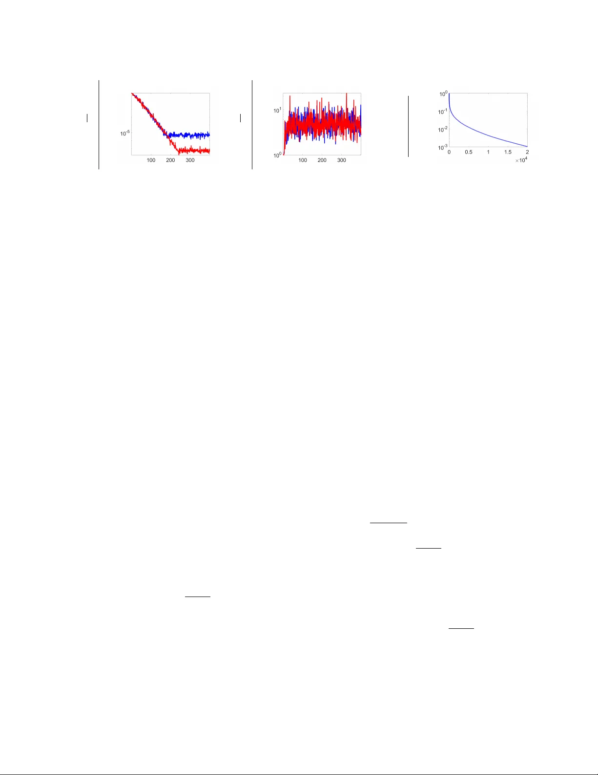
1 Con v er gence and sample complexity of gradient methods for the model-free linear quadratic re gulator problem Hesameddin Mohammadi, Armin Zare, Mahdi Soltanolkotabi, and Mihailo R. Jo vano vi ´ c Abstract Model-free reinforcement learning attempts to ﬁnd an optimal control action for an unknown dynamical system by directly searching ov er the parameter space of controllers. The conv ergence behavior and statistical properties of these approaches are often poorly understood because of the noncon ve x nature of the underlying optimization problems and the lack of exact gradient computation. In this paper, we take a step towards demystifying the performance and efﬁciency of such methods by focusing on the standard inﬁnite-horizon linear quadratic regulator problem for continuous-time systems with unknown state-space parameters. W e establish exponential stability for the ordinary differential equation (ODE) that governs the gradient-ﬂow dynamics over the set of stabilizing feedback gains and show that a similar result holds for the gradient descent method that arises from the forward Euler discretization of the corresponding ODE. W e also provide theoretical bounds on the conv ergence rate and sample complexity of the random search method with two-point gradient estimates. W e prove that the required simulation time for achieving  -accuracy in the model-free setup and the total number of function e valuations both scale as log (1 / ) . Index T erms Data-driv en control, gradient descent, gradient-ﬂow dynamics, linear quadratic regulator , model-free control, noncon ve x optimization, Polyak-Lojasiewicz inequality , random search method, reinforcement learning, sample complexity . I . I N T RO D U C T I O N In many emerging applications, control-oriented models are not readily av ailable and classical approaches from optimal control may not be directly applicable. This challenge has led to the emergence of Reinforcement Learning (RL) approaches that often perform well in practice. Examples include learning complex locomotion tasks via neural network dynamics [1] and playing Atari games based on images using deep-RL [2]. RL approaches can be broadly divided into model-based [3], [4] and model-free [5], [6]. While model-based RL uses data to obtain approximations of the underlying dynamics, its model-free counterpart prescribes control actions based on estimated values of a cost function without attempting to form a model. In spite of the empirical success of RL in a variety of domains, our mathematical understanding of it is still in its infancy and there are many open questions surrounding con ver gence and sample complexity . In this paper, we take a step tow ards answering such questions with a focus on the inﬁnite-horizon Linear Quadratic Regulator (LQR) for continuous-time systems. The w ork of H. Mohammadi, A. Zare, and M. R. Jov anovi ´ c is supported in part by the National Science Foundation (NSF) under A wards ECCS-1708906 and ECCS-1809833 and the Air Force Ofﬁce of Scientiﬁc Research (AFOSR) under A ward F A9550-16-1-0009. The work of M. Soltanolkotabi is supported in part by the Packard Fellowship in Science and Engineering, a Sloan Research Fello wship in Mathematics, a Google Faculty Research A ward, as well as A wards from NSF , Darpa LwLL program, and AFOSR Y oung In vestigator Program. H. Mohammadi, M. Soltanolkotabi, and M. R. Jov anovi ´ c are with the Ming Hsieh Department of Electrical and Computer Engineering, Univ ersity of Southern California, Los Angeles, CA 90089. A. Zare is with the Department of Mechanical Engineering, Univ ersity of T e xas at Dallas, Richardson, TX 75080. Emails: { hesamedm, soltanol, mihailo } @usc.edu, armin.zare@utdallas.edu. March 17, 2021 DRAFT 2 The LQR problem is the cornerstone of control theory . The globally optimal solution can be obtained by solving the Riccati equation and efﬁcient numerical schemes with prov able con ver gence guarantees hav e been de veloped [7]. Howe v er , computing the optimal solution becomes challenging for large-scale problems, when prior kno wledge is not available, or in the presence of structural constraints on the controller . This motiv ates the use of direct search methods for controller synthesis. Unfortunately , the noncon ve x nature of this formulation complicates the analysis of ﬁrst- and second-order optimization algorithms. T o make matters worse, structural constraints on the feedback gain matrix may result in a disjoint search landscape limiting the utility of con ventional descent-based methods [8]. Furthermore, in the model-free setting, the exact model (and hence the gradient of the objective function) is unknown so that only zeroth-order methods can be used. In this paper, we study con v ergence properties of gradient-based methods for the continuous-time LQR problem. In spite of the lack of con v exity , we establish (a) e xponential stability of the ODE that gov erns the gradient-ﬂow dynamics over the set of stabilizing feedback gains; and (b) linear conver gence of the gradient descent algorithm with a suitable stepsize. W e employ a standard con ve x reparameterization for the LQR problem [9], [10] to establish the con v ergence properties of gradient-based methods for the noncon ve x formulation. In the model-free setting, we also examine con ver gence and sample complexity of the random search method [11] that attempts to emulate the behavior of gradient descent via gradient approximations resulting from objective function values. For the two-point gradient estimation setting, we prov e linear conv ergence of the random search method and show that the total number of function ev aluations and the simulation time required in our results to achieve  -accuracy are proportional to log (1 / ) . For the discr ete-time LQR, global con ver gence guarantees were recently provided in [12] for gradient decent and the random search method with one-point gradient estimates. The authors established a bound on the sample complexity for reaching the error tolerance  that requires a number of function ev aluations that is at least proportional to (1 / 4 ) log (1 / ) . If one has access to the inﬁnite-horizon cost v alues, the number of function ev aluations for the random search method with one-point gradient estimates can be improved to 1 / 2 [13]. In contrast, we focus on the continuous-time LQR and examine the two-point gradient estimation setting. The use of two-point gradient estimates reduces the required number of function ev aluations to 1 / [13]. W e signiﬁcantly improv e this result by showing that the required number of function ev aluations is proportional to log (1 / ) . Similarly , the simulation time required in our results is proportional to log (1 / ) ; this is in contrast to [12] that requires p oly (1 / ) simulation time and [13] that assumes an inﬁnite simulation time. Furthermore, our con ver gence results hold both in terms of the error in the objecti ve value and the optimization v ariable (i.e., the feedback gain matrix) whereas [12] and [13] only prov e con ver gence in the objective value. W e note that the literature on model-free RL is rapidly expanding and recent extensions to Markovian jump linear systems [14], H ∞ robustness analysis through implicit regularization [15], learning distrib uted LQ problems [16], and output-feedback LQR [17] hav e been made. Our presentation is structured as follows. In Section II, we revisit the LQR problem and present gradient-ﬂow dynamics, gradient descent, and the random search algorithm. In Section III, we highlight the main results of the paper . In Section IV, we utilize conv ex reparameterization of the LQR problem and establish exponential stability of the resulting gradient-ﬂow dynamics and gradient descent method. In Section V, we extend our analysis to the noncon ve x landscape of feedback gains. In Section VI, we quantify the accuracy of two-point gradient estimates and, in Section VII, we discuss con ver gence and sample complexity of the random search method. In Section VIII, March 17, 2021 DRAFT 3 we provide an example to illustrate our theoretical dev elopments and, in Section IX, we offer concluding remarks. Most technical details are relegated to the appendices. Notation: W e use v ec( M ) ∈ R mn to denote the vectorized form of the matrix M ∈ R m × n obtained by concatenating the columns on top of each other . W e use k M k 2 F = h M , M i to denote the Frobenius norm, where h X, Y i : = trace ( X T Y ) is the standard matricial inner product. W e denote the largest singular v alue of linear operators and matrices by k · k 2 and the spectral induced norm of linear operators by k · k S kMk 2 : = sup M kM ( M ) k F k M k F , kMk S : = sup M kM ( M ) k 2 k M k 2 . W e denote by S n ⊂ R n × n the set of symmetric matrices. For M ∈ S n , M  0 means M is positive deﬁnite and λ min ( M ) is the smallest eigen value. W e use S d − 1 ⊂ R d to denote the unit sphere of dimension d − 1 . W e denote the expected value by E [ · ] and probability by P ( · ) . T o compare the asymptotic beha vior of f (  ) and g (  ) as  goes to 0 , we use f = O ( g ) (or , equiv alently , g = Ω( f ) ) to denote lim sup  → 0 f (  ) /g (  ) < ∞ ; f = ˜ O ( g ) to denote f = O ( g log k g ) for some integer k ; and f = o (  ) to signify lim  → 0 f (  ) / = 0 . I I . P RO B L E M F O R M U L ATI O N The inﬁnite-horizon LQR problem for continuous-time L TI systems is given by minimize x, u E  Z ∞ 0 ( x T ( t ) Qx ( t ) + u T ( t ) Ru ( t )) d t  (1a) sub ject to ˙ x = Ax + B u, x (0) ∼ D (1b) where x ( t ) ∈ R n is the state, u ( t ) ∈ R m is the control input, A and B are constant matrices of appropriate dimensions, Q and R are positive deﬁnite matrices, and the expectation is taken over a random initial condition x (0) with distribution D . For a controllable pair ( A, B ) , the solution to (1) is giv en by u ( t ) = − K ? x ( t ) = − R − 1 B T P ? x ( t ) (2a) where P ? is the unique positiv e deﬁnite solution to the Algebraic Riccati Equation (ARE) A T P ? + P ? A + Q − P ? B R − 1 B T P ? = 0 . (2b) When the model is known, the LQR problem and the corresponding ARE can be solved efﬁciently via a variety of techniques [18]–[21]. Howe ver , these methods are not directly applicable in the model-free setting, i.e., when the matrices A and B are unknown. Exploiting the linearity of the optimal controller , we can alternativ ely formulate the LQR problem as a direct search for the optimal linear feedback gain, namely minimize K f ( K ) (3a) where f ( K ) : = ( trace  ( Q + K T R K ) X ( K )  , K ∈ S K ∞ , otherwise. (3b) March 17, 2021 DRAFT 4 Here, the function f ( K ) determines the LQR cost in (1a) associated with the linear state-feedback law u = − K x , S K : = { K ∈ R m × n | A − B K is Hurwitz } (3c) is the set of stabilizing feedback gains and, for any K ∈ S K , X ( K ) : = Z ∞ 0 E  x ( t ) x T ( t )  = Z ∞ 0 e ( A − B K ) t Ω e ( A − B K ) T t d t (4a) is the unique solution to the L yapunov equation ( A − B K ) X + X ( A − B K ) T + Ω = 0 (4b) and Ω : = E [ x (0) x T (0)] . T o ensure f ( K ) = ∞ for K / ∈ S K , we assume Ω  0 . This assumption also guarantees K ∈ S K if and only if the solution X to (4b) is positive deﬁnite. In problem (3) , the matrix K is the optimization variable, and ( A , B , Q  0 , R  0 , Ω  0 ) are the problem parameters. This alternativ e formulation of the LQR problem has been studied for both continuous-time [7] and discrete-time systems [12], [22] and it serves as a building block for several important control problems including optimal static-output feedback design [23], optimal design of sparse feedback gain matrices [24]–[27], and optimal sensor/actuator selection [28]–[30]. For all stabilizing feedback gains K ∈ S K , the gradient of the objecti ve function is determined by [23], [24] ∇ f ( K ) = 2( R K − B T P ( K )) X ( K ) . (5) Here, X ( K ) is giv en by (4a) and P ( K ) = Z ∞ 0 e ( A − B K ) T t ( Q + K T R K ) e ( A − B K ) t d t (6a) is the unique positiv e deﬁnite solution of ( A − B K ) T P + P ( A − B K ) = − Q − K T R K. (6b) T o simplify our presentation, for any K ∈ R m × n , we deﬁne the closed-loop L yapuno v operator A K : S n → S n as A K ( X ) : = ( A − B K ) X + X ( A − B K ) T . (7a) For K ∈ S K , both A K and its adjoint A ∗ K ( P ) = ( A − B K ) T P + P ( A − B K ) (7b) are in v ertible and X ( K ) , P ( K ) are determined by X ( K ) = −A − 1 K (Ω) , P ( K ) = − ( A ∗ K ) − 1 ( Q + K T RK ) . In this paper, we ﬁrst examine the global stability properties of the gradient-ﬂow dynamics ˙ K = −∇ f ( K ) , K (0) ∈ S K (GF) March 17, 2021 DRAFT 5 associated with problem (3) and its discretized variant, K k +1 : = K k − α ∇ f ( K k ) , K 0 ∈ S K (GD) where α > 0 is the stepsize. Next, we use this analysis as a building block to study the con ver gence of a search method based on random sampling [11], [31] for solving problem (3) . As described in Algorithm 1, at each iteration we form an empirical approximation ∇ f ( K ) to the gradient of the objective function via simulation of system (1b) for randomly perturbed feedback gains K ± U i , i = 1 , . . . , N , and update K via, K k +1 : = K k − α ∇ f ( K k ) , K 0 ∈ S K . (RS) W e note that the gradient estimation scheme in Algorithm 1 does not require knowledge of system matrices A and B in (1b) but only access to a simulation engine. Algorithm 1 T wo-point gradient estimation Input: Feedback gain K ∈ R m × n , state and control weight matrices Q and R , distribution D , smoothing constant r , simulation time τ , number of random samples N . for i = 1 , . . . , N do – Deﬁne perturbed feedback gains K i, 1 : = K + rU i and K i, 2 : = K − rU i , where v ec( U i ) is a random vector uniformly distrib uted on the sphere √ mn S mn − 1 . – Sample an initial condition x i from distrib ution D . – For j ∈ { 1 , 2 } , simulate system (1b) up to time τ with the feedback gain K i,j and initial condition x i to form ˆ f i,j = Z τ 0 ( x T ( t ) Qx ( t ) + u T ( t ) Ru ( t )) d t . end f or Output: The gradient estimate ∇ f ( K ) = 1 2 r N N X i = 1  ˆ f i, 1 − ˆ f i, 2  U i . I I I . M A I N R E S U LT S Optimization problem (3) is not con v ex [8]; see Appendix A for an example. The function f ( K ) , howe ver , has two important properties: uniqueness of the critical points and the compactness of sublevel sets [32], [33]. Based on these, the LQR objective error f ( K ) − f ( K ? ) can be used as a maximal L yapuno v function (see [34] for a deﬁnition) to prove asymptotic stability of gradient-ﬂow dynamics (GF) ov er the set of stabilizing feedback gains S K . Howe ver , this approach does not provide any guarantee on the rate of con v ergence and additional analysis is necessary to establish exponential stability; see Section V for details. A. Known model W e ﬁrst summarize our results for the case when the model is known. In spite of the nonconv ex optimization landscape, we establish the exponential stability of gradient-ﬂo w dynamics (GF) for any stabilizing initial feedback gain K (0) . This result also provides an explicit bound on the rate of con v ergence to the LQR solution K ? . Theor em 1: For any initial stabilizing feedback gain K (0) ∈ S K , the solution K ( t ) to gradient-ﬂow dynamics (GF) March 17, 2021 DRAFT 6 satisﬁes f ( K ( t )) − f ( K ? ) ≤ e − ρ t ( f ( K (0)) − f ( K ? )) k K ( t ) − K ? k 2 F ≤ b e − ρ t k K (0) − K ? k 2 F where the conv er gence rate ρ and constant b depend on K (0) and the parameters of the LQR problem (3). The proof of Theorem 1 along with explicit expressions for the con ver gence rate ρ and constant b are provided in Section V -A . Moreover , for a sufﬁciently small stepsize α , we show that gradient descent method (GD) also con ver ges over S K at a linear rate. Theor em 2: For any initial stabilizing feedback gain K 0 ∈ S K , the iterates of gradient descent (GD) satisfy f ( K k ) − f ( K ? ) ≤ γ k  f ( K 0 ) − f ( K ? )  k K k − K ? k 2 F ≤ b γ k k K 0 − K ? k 2 F where the rate of con ver gence γ , stepsize α , and constant b depend on K 0 and the parameters of the LQR problem (3) . B. Unknown model W e no w turn our attention to the model-free setting. W e use Theorem 2 to carry out the con ver gence analysis of the random search method (RS) under the following assumption on the distribution of initial condition. Assumption 1: Let the distribution D of the initial conditions have i.i.d. zero-mean unit-variance entries with bounded sub-Gaussian norm, i.e., for a random vector v ∈ R n distributed according to D , E [ v i ] = 0 and k v i k ψ 2 ≤ κ , for some constant κ and i = 1 , . . . , n ; see Appendix J for the deﬁnition of k · k ψ 2 . Our main con v ergence result holds under Assumption 1. Speciﬁcally , for a desired accuracy lev el  > 0 , in Theorem 3 we establish that iterates of (RS) with constant stepsize (that does not depend on  ) reach accuracy level  at a linear rate (i.e., in at most O (log (1 / )) iterations) with high probability . Furthermore, the total number of function ev aluations and the simulation time required to achieve an accuracy level  are proportional to log (1 / ) . This signiﬁcantly improv es the existing results for discrete-time LQR [12], [13] that require O (1 / ) function e valuations and poly (1 / ) simulation time. Theor em 3 (Informal): Let the initial condition x 0 ∼ D of system (1b) obey Assumption 1. Also let the simulation time τ and the number of samples N in Algorithm 1 satisfy τ ≥ θ 1 log (1 / ) and N ≥ c  1 + β 4 κ 4 θ 1 log 6 n  n for some β > 0 and desired accuracy  > 0 . Then, we can choose the smoothing parameter r < θ 3 √  in Algorithm 1 and the constant stepsize α such that the random search method (RS) that starts from any initial stabilizing feedback gain K 0 ∈ S K achiev es f ( K k ) − f ( K ? ) ≤  in at most k ≤ θ 4 log  ( f ( K 0 ) − f ( K ? )) /  iterations with probability not smaller than 1 − c 0 k ( n − β + N − β + N e − n 8 + e − c 0 N ) . Here, the positive scalars c and c 0 are absolute constants and θ 1 , . . . , θ 4 > 0 depend on K 0 and the parameters of the LQR problem (3). The formal version of Theorem 3 along with a discussion of parameters θ i and stepsize α is presented in Section VII. March 17, 2021 DRAFT 7 I V . C O N V E X R E PA R A M ET E R I Z AT I O N The main challenge in establishing the exponential stability of (GF) arises from noncon v exity of problem (3) . Herein, we use a standard change of variables to reparameterize (3) into a conv ex problem, for which we can provide exponential stability guarantees for gradient-ﬂow dynamics. W e then connect the gradient ﬂow on this con ve x reparameterization to its noncon v ex counterpart and establish the exponential stability of (GF). A. Change of variables The stability of the closed-loop system with the feedback gain K ∈ S K in problem (3) is equiv alent to the positiv e deﬁniteness of the matrix X ( K ) giv en by (4a) . This condition allo ws for a standard change of v ariables K = Y X − 1 , for some Y ∈ R m × n , to reformulate the LQR design as a con ve x optimization problem [9], [10]. In particular , for any K ∈ S K and the corresponding matrix X , we have f ( K ) = h ( X, Y ) : = trace ( Q X + Y T R Y X − 1 ) where h ( X, Y ) is a jointly con v ex function of ( X, Y ) for X  0 . In the ne w variables, L yapuno v equation (4b) takes the afﬁne form A ( X ) − B ( Y ) + Ω = 0 (8a) where A and B are the linear maps A ( X ) : = A X + X A T , B ( Y ) : = B Y + Y T B T . (8b) For an in vertible map A , we can express the matrix X as an afﬁne function of Y X ( Y ) = A − 1 ( B ( Y ) − Ω) (8c) and bring the LQR problem into the con ve x form minimize Y h ( Y ) (9) where h ( Y ) : = ( h ( X ( Y ) , Y ) , Y ∈ S Y ∞ , otherwise and S Y : = { Y ∈ R m × n | X ( Y )  0 } is the set of matrices Y that correspond to stabilizing feedback gains K = Y X − 1 . The set S Y is open and con v ex because it is deﬁned via a positi v e deﬁnite condition imposed on the afﬁne map X ( Y ) in (8c) . This positiv e deﬁnite condition in S Y is equiv alent to the closed-loop matrix A − B Y ( X ( Y )) − 1 being Hurwitz. Remark 1: Although our presentation assumes in v ertibility of A , this assumption comes without loss of generality . As shown in Appendix B, all results carry ov er to nonin vertible A with an alternativ e change of variables A = ˆ A + B K 0 , K = ˆ K + K 0 , and ˆ K = ˆ Y X − 1 , for some K 0 ∈ S K . B. Smoothness and str ong con vexity of h ( Y ) Our con v ergence analysis of gradient methods for problem (IV -A) relies on the L -smoothness and µ -strong con ve xity of the function h ( Y ) ov er its sublev el sets S Y ( a ) : = { Y ∈ S Y | h ( Y ) ≤ a } . These two properties March 17, 2021 DRAFT 8 were recently established in [30] where it was shown that ov er any sublev el set S Y ( a ) , the second-order term D ˜ Y , ∇ 2 h ( Y ; ˜ Y ) E in the T aylor series expansion of h ( Y + ˜ Y ) around Y ∈ S Y ( a ) can be upper and lo wer bounded by quadratic forms L k ˜ Y k 2 F and µ k ˜ Y k 2 F for some positi ve scalars L and µ . While an explicit form for the smoothness parameter L along with an existence proof for the strong con ve xity modulus µ were presented in [30], in Proposition 1 we establish an explicit expression for µ in terms of a and parameters of the LQR problem. This allows us to provide bounds on the conv ergence rate for gradient methods. Pr oposition 1: Over any non-empty sublev el set S Y ( a ) , the function h ( Y ) is L -smooth and µ -strongly conv ex with L = 2 a k R k 2 ν 1 + a kA − 1 B k 2 p ν λ min ( R ) ! 2 (10a) µ = 2 λ min ( R ) λ min ( Q ) a (1 + a 2 η ) 2 (10b) where the constants η : = kB k 2 λ min ( Q ) λ min (Ω) p ν λ min ( R ) (10c) ν : = λ 2 min (Ω) 4 k A k 2 p λ min ( Q ) + k B k 2 p λ min ( R ) ! − 2 (10d) only depend on the problem parameters. Pr oof: See Appendix C. C. Gr adient methods over S Y The LQR problem can be solved by minimizing the con ve x function h ( Y ) whose gradient is giv en by [30, Appendix C] ∇ h ( Y ) = 2 R Y ( X ( Y )) − 1 − 2 B T W ( Y ) (11a) where W ( Y ) is the solution to A T W + W A = ( X ( Y )) − 1 Y T R Y ( X ( Y )) − 1 − Q. (11b) Using the strong conv exity and smoothness properties of h ( Y ) established in Proposition 1, we next show that the unique minimizer Y ? of the function h ( Y ) is the exponentially stable equilibrium point of the gradient-ﬂow dynamics ov er S Y , ˙ Y = −∇ h ( Y ) , Y (0) ∈ S Y . (GFY) Pr oposition 2: For any Y (0) ∈ S Y , the gradient-ﬂow dynamics (GFY) are exponentially stable, i.e., k Y ( t ) − Y ? k 2 F ≤ ( L/µ ) e − 2 µ t k Y (0) − Y ? k 2 F where µ and L are the strong con v exity and smoothness parameters of the function h ( Y ) ov er the sublev el set S Y ( h ( Y (0))) . March 17, 2021 DRAFT 9 Pr oof: The deri vati v e of the L yapuno v function candidate V ( Y ) : = h ( Y ) − h ( Y ? ) along the ﬂow in (GFY) satisﬁes ˙ V = D ∇ h ( Y ) , ˙ Y E = −k∇ h ( Y ) k 2 F ≤ − 2 µV . (12) Inequality (12) is a consequence of the strong con ve xity of h ( Y ) and it yields [35, Lemma 3.4] V ( Y ( t )) ≤ e − 2 µ t V ( Y (0)) . (13) Thus, for any Y (0) ∈ S Y , h ( Y ( t )) con ver ges exponentially to h ( Y ? ) . Moreover , since h ( Y ) is µ -strongly conv ex and L -smooth, V ( Y ) can be upper and lower bounded by quadratic functions and the exponential stability of (GFY) ov er S Y follows from L yapunov theory [35, Theorem 4.10]. In Section V, we use the abov e result to prov e exponential/linear con v ergence of gradient ﬂow/descent for the noncon ve x optimization problem (3) . Before we proceed, we note that similar conv ergence guarantees can be established for the gradient descent method with a sufﬁciently small stepsize α , Y k +1 : = Y k − α ∇ h ( Y k ) , Y 0 ∈ S Y (GY) Since the function h ( Y ) is L -smooth ov er the sublev el set S Y ( h ( Y 0 )) , for any α ∈ [0 , 1 /L ] the iterates Y k remain within S Y ( h ( Y 0 )) . This property in conjunction with the µ -strong con v exity of h ( Y ) imply that Y k con ver ges to the optimal solution Y ? at a linear rate of γ = 1 − α µ . V . C O N T RO L D E S I G N W I T H A K N OW N M O D E L The asymptotic stability of (GF) is a consequence of the following properties of the LQR objective function [32], [33]: 1) The function f ( K ) is twice continuously differentiable over its open domain S K and f ( K ) → ∞ as K → ∞ and/or K → ∂ S K . 2) The optimal solution K ? is the unique equilibrium point ov er S K , i.e., ∇ f ( K ) = 0 if and only if K = K ? . In particular , the deri v ati ve of the maximal L yapunov function candidate V ( K ) : = f ( K ) − f ( K ? ) along the trajectories of (GF) satisﬁes ˙ V = D ∇ f ( K ) , ˙ K E = −k∇ f ( K ) k 2 F ≤ 0 where the inequality is strict for all K 6 = K ? . Thus, L yapuno v theory [34] implies that, starting from any stabilizing initial condition K (0) , the trajectories of (GF) remain within the suble vel set S K ( f ( K (0))) and asymptotically con ver ge to K ? . Similar arguments were employed for the con ver gence analysis of the Anderson-Moore algorithm for output- feedback synthesis [32]. While [32] shows global asymptotic stability , it does not provide any information on the rate of con v ergence. In this section, we ﬁrst demonstrate exponential stability of (GF) and prov e Theorem 1. Then, we establish linear con ver gence of the gradient descent method (GD) and prov e Theorem 2. A. Gr adient-ﬂow dynamics: pr oof of Theorem 1 W e start our proof of Theorem 1 by relating the con ve x and noncon ve x formulations of the LQR objective function. Speciﬁcally , in Lemma 1, we establish a relation between the gradients ∇ f ( K ) and ∇ h ( Y ) ov er the sublevel sets March 17, 2021 DRAFT 10 of the objective function S K ( a ) : = { K ∈ S K | f ( K ) ≤ a } . Lemma 1: For any stabilizing feedback gain K ∈ S K ( a ) and Y : = K X ( K ) , we hav e k∇ f ( K ) k F ≥ c k∇ h ( Y ) k F (14a) where X ( K ) is giv en by (4a), the constant c is determined by c = ν p ν λ min ( R ) 2 a 2 kA − 1 k 2 k B k 2 + a p ν λ min ( R ) (14b) and the scalar ν giv en by Eq. (10d) depends on the problem parameters. Pr oof: See Appendix D. Using Lemma 1 and the exponential stability of gradient-ﬂo w dynamics (GFY) ov er S Y , established in Proposition 2, we next show that (GF) is also exponentially stable. In particular , for any stabilizing K ∈ S K ( a ) , the deriv ativ e of V ( K ) : = f ( K ) − f ( K ? ) along the gradient ﬂow in (GF) satisﬁes ˙ V = −k∇ f ( K ) k 2 F ≤ − c 2 k∇ h ( Y ) k 2 F ≤ − 2 µ c 2 V (15) where Y = K X ( K ) and the constants c and µ are provided in Lemma 1 and Proposition 1, respectiv ely . The ﬁrst inequality in (15) follo ws from (14a) and the second follows from f ( K ) = h ( Y ) combined with k∇ h ( Y ) k 2 F ≥ 2 µV (which in turn is a consequence of the strong con v exity of h ( Y ) established in Proposition 1). Now , since the sublev el set S K ( a ) is in v ariant with respect to (GF) , follo wing [35, Lemma 3.4], inequality (15) guarantees that system (GF) con ver ges exponentially in the objective value with rate ρ = 2 µc 2 . This concludes the proof of part (a) in Theorem 1. In order to prove part (b), we use the following lemma which connects the errors in the objecti ve value and the optimization variable. Lemma 2: For any stabilizing feedback gain K , the objecti ve function f ( K ) in problem (3) satisﬁes f ( K ) − f ( K ? ) = trace  ( K − K ? ) T R ( K − K ? ) X ( K )  where K ? is the optimal solution and X ( K ) is giv en by (4a). Pr oof: See Appendix D. From Lemma 2 and part (a) of Theorem 1, we have k K ( t ) − K ? k 2 F ≤ f ( K ( t )) − f ( K ? ) λ min ( R ) λ min ( X ( K ( t ))) ≤ e − ρ t f ( K (0)) − f ( K ? ) λ min ( R ) λ min ( X ( K ( t ))) ≤ b 0 e − ρ t k K (0) − K ? k 2 F where b 0 : = k R k 2 k X ( K (0)) k 2 / ( λ min ( R ) λ min ( X ( K ( t )))) . Here, the ﬁrst and third inequalities follow form basic properties of the matrix trace combined with Lemma 2 applied with K = K ( t ) and K = K (0) , respectively . The second inequality follows from part (a) of Theorem 1. Finally , to upper bound parameter b 0 , we use Lemma 23 presented in Appendix K that provides the lower and upper bounds ν /a ≤ λ min ( X ( K )) and k X ( K ) k 2 ≤ a/λ min ( Q ) on the matrix X ( K ) for any K ∈ S K ( a ) , where the constant ν is gi ven by (10d) . Using these bounds and the in v ariance of S K ( a ) with respect to (GF) , we obtain b 0 ≤ b : = a 2 k R k 2 ν λ min ( R ) λ min ( Q ) (16) which completes the proof of part (b). March 17, 2021 DRAFT 11 Remark 2 (Gradient domination): Expression (15) implies that the objectiv e function f ( K ) ov er any gi ven sublev el set S K ( a ) satisﬁes the Polyak-Łojasiewicz (PL) condition [36] k∇ f ( K ) k 2 F ≥ 2 µ f ( f ( K ) − f ( K ? )) (17) with parameter µ f : = µ c 2 , where µ and c are functions of a that are given by (10b) and (14b) , respecti vely . This condition is also known as gradient dominance and it was recently used to sho w con ver gence of gradient-based methods for discrete-time LQR problem [12]. B. Geometric interpr etation The solution Y ( t ) to gradient-ﬂo w dynamics (GFY) over the set S Y induces the trajectory K ind ( t ) : = Y ( t )( X ( Y ( t ))) − 1 (18) ov er the set of stabilizing feedback gains S K , where the af ﬁne function X ( Y ) is gi ven by (8c) . The induced trajectory K ind ( t ) can be viewed as the solution to the differential equation ˙ K = g ( K ) (19a) where g : S K → R m × n is gi ven by g ( K ) : =  K A − 1 ( B ( ∇ h ( Y ( K )))) − ∇ h ( Y ( K ))  ( X ( K )) − 1 . (19b) Here, the matrix X = X ( K ) is giv en by (4a) and Y ( K ) = K X ( K ) . System (19) is obtained by differentiating both sides of Eq. (18) with respect to time t and applying the chain rule. Figure 1 illustrates an induced trajectory K ind ( t ) and a trajectory K ( t ) resulting from gradient-ﬂow dynamics (GF) that starts from the same initial condition. Moreov er , using the deﬁnition of h ( Y ) , we hav e h ( Y ( t )) = f ( K ind ( t )) . (20) Thus, the exponential decay of h ( Y ( t )) established in Proposition 2 implies that f decays exponentially along the vector ﬁeld g , i.e., for K ind (0) 6 = K ? , we have f ( K ind ( t )) − f ( K ? ) f ( K ind (0)) − f ( K ? ) = h ( Y ( t )) − h ( Y ? ) h ( Y (0)) − h ( Y ? ) ≤ e − 2 µ t . This inequality follows from inequality (13) , where µ denotes the strong-con ve xity modulus of the function h ( Y ) ov er the suble vel set S Y ( h ( Y (0))) ; see Proposition 1. Herein, we provide a geometric interpretation of the exponential decay of f under the trajectories of (GF) that is based on the relation between the vector ﬁelds g and −∇ f . Differentiating both sides of Eq. (20) with respect to t yields k∇ h ( Y ) k 2 = h−∇ f ( K ) , g ( K ) i . (21) Thus, for each K ∈ S K , the inner product between the vector ﬁelds −∇ f ( K ) and g ( K ) is nonneg ativ e. Howe ver , this is not sufﬁcient to ensure exponential decay of f along (GF) . T o address this challenge, our proof utilizes March 17, 2021 DRAFT 12 K 0 K  Fig. 1. T rajectories K ( t ) of (GF) (solid black) and K ind ( t ) resulting from Eq. (18) (dashed blue) along with the lev el sets of the function f ( K ) . inequality (14a) in Lemma 1. Based on (21), (14a) can be equiv alently restated as k − ∇ f ( K ) k F k Π −∇ f ( K ) ( g ( K )) k F = k∇ f ( K ) k 2 F h−∇ f ( K ) , g ( K ) i ≥ c 2 where Π b ( a ) denotes the projection of a onto b . Thus, Lemma 1 ensures that the ratio between the norm of the vector ﬁeld −∇ f ( K ) associated with gradient-ﬂow dynamics (GF) and the norm of the projection of g ( K ) onto −∇ f ( K ) is uniformly lower bounded by a positiv e constant. This lo wer bound is the key geometric feature that allows us to deduce exponential decay of f along the vector ﬁeld −∇ f from the exponential decay of the vector ﬁeld g . C. Gr adient descent: pr oof of Theorem 2 Gi ven the exponential stability of gradient-ﬂow dynamics (GF) established in Theorem 1, the con ver gence analysis of gradient descent (GD) amounts to ﬁnding a suitable stepsize α . Lemma 3 provides a Lipschitz continuity parameter for ∇ f ( K ) , which facilitates ﬁnding such a stepsize. Lemma 3: Over any non-empty suble vel set S K ( a ) , the gradient ∇ f ( K ) is Lipschitz continuous with parameter L f : = 2 a k R k 2 λ min ( Q ) + 8 a 3 k B k 2 λ 2 min ( Q ) λ min (Ω)  k B k 2 λ min (Ω) + k R k 2 p ν λ min ( R )  where ν given by (10d) depends on the problem parameters. Pr oof: See Appendix D. Let K α : = K − α ∇ f ( K ) , α ≥ 0 parameterize the half-line starting from K ∈ S K ( a ) with K 6 = K ? along −∇ f ( K ) and let us deﬁne the scalar β m : = max β such that K α ∈ S K ( a ) , for all α ∈ [0 , β ] . The existence of β m follows from the compactness of S K ( a ) [32]. W e next show that β m ≥ 2 /L f . For the sake of contradiction, suppose β m < 2 /L f . From the continuity of f ( K α ) with respect to α , it follows that f ( K β s ) = a . Moreover , since −∇ f ( K ) is a descent direction of the function f ( K ) , we hav e β m > 0 . Thus, for α ∈ (0 , β m ] , f ( K α ) − f ( K ) ≤ − α (2 − L f α ) 2 k∇ f ( K ) k 2 F < 0 . Here, the ﬁrst inequality follows from the L f -smoothness of f ( K ) ov er S K ( a ) (Descent Lemma [37, Eq. (9.17)]) and the second inequality follows from ∇ f ( K ) 6 = 0 in conjunction with β m ∈ (0 , 2 /L f ) . This implies f ( K β m ) < f ( K ) ≤ a , which contradicts f ( K β m ) = a . Thus, β m ≥ 2 /L f . March 17, 2021 DRAFT 13 W e can no w use induction on k to show that, for any stabilizing initial condition K 0 ∈ S K ( a ) , the iterates of (GD) with α ∈ [0 , 2 /L f ] remain in S K ( a ) and satisfy f ( K k +1 ) − f ( K k ) ≤ − α (2 − L f α ) 2 k∇ f ( K k ) k 2 F . (22) Inequality (22) in conjunctions with the PL condition (17) e valuated at K k guarantee linear conv er gence for gradient descent (GD) with the rate γ ≤ 1 − α µ f for all α ∈ (0 , 1 /L f ] , where µ f is the PL parameter of the function f ( K ) . This completes the proof of part (a) of Theorem 2. Using part (a) and Lemma 2, we can make a similar argument to what we used for the proof of Theorem 1 to establish part (b) with constant b in (16). W e omit the details for brevity . Remark 3: Using our results, it is straightforward to show linear con v ergence of K k +1 = K k − αH k 1 ∇ f ( K k ) H k 2 with K 0 ∈ S K and small enough stepsize, where H k 1 and H k 2 are uniformly upper and lo wer bounded positi ve deﬁnite matrices. In particular , the Kleinman iteration [18] is recovered for α = 0 . 5 , H k 1 = R − 1 , and H k 2 = ( X ( K k )) − 1 . Similarly , con ver gence of gradient descent may be improv ed by choosing H k 1 = I and H k 2 = ( X ( K k )) − 1 . In this case, the corresponding update direction provides the continuous-time variant of the so-called natural gradient for discrete-time systems [38]. V I . B I A S A N D C O R R E L A T I O N I N G R A D I E N T E S T I M A T I O N In the model-free setting, we do not hav e access to the gradient ∇ f ( K ) and the random search method (RS) relies on the gradient estimate ∇ f ( K ) resulting from Algorithm 1. According to [12], achieving k∇ f ( K ) − ∇ f ( K ) k F ≤  may take N = Ω(1 / 4 ) samples using one-point gradient estimates. Our computational experiments (not included in this paper) also suggest that to achiev e k∇ f ( K ) − ∇ f ( K ) k F ≤  , N must scale as p oly (1 / ) ev en when a two-point gradient estimate is used. T o avoid this poor sample complexity , in our proof we take an alternativ e route and give up on the objectiv e of controlling the gradient estimation error . By exploiting the problem structure, we show that with a linear number of samples N = ˜ O ( n ) , where n is the number of states, the estimate ∇ f ( K ) concentrates with high pr obability when projected to the direction of ∇ f ( K ) . Our proof strategy allows us to signiﬁcantly improv e upon the existing literature both in terms of the required function ev aluations and simulation time. Speciﬁcally , using the random search method (RS) , the total number of function ev aluations required in our results to achie ve an accuracy lev el  is proportional to log (1 / ) compared to at least (1 / 4 ) log (1 / ) in [12] and 1 / in [13]. Similarly , the simulation time that we require to achie ve an accuracy lev el  is proportional to log (1 / ) ; this is in contrast to p oly (1 / ) simulation times in [12] and inﬁnite simulation time in [13]. Algorithm 1 produces a biased estimate ∇ f ( K ) of the gradient ∇ f ( K ) . Herein, we ﬁrst introduce an unbiased estimate b ∇ f ( K ) of ∇ f ( K ) and establish that the distance k b ∇ f ( K ) − ∇ f ( K ) k F can be readily controlled by choosing a large simulation time τ and an appropriate smoothing parameter r in Algorithm 1; we call this distance the estimation bias. Next, we show that with N = ˜ O ( n ) samples, the unbiased estimate b ∇ f ( K ) becomes highly correlated with ∇ f ( K ) . W e exploit this fact in our con v ergence analysis. March 17, 2021 DRAFT 14 A. Bias in gradient estimation due to ﬁnite simulation time W e ﬁrst introduce an unbiased estimate of the gradient that is used to quantify the bias. For any τ ≥ 0 and x 0 ∈ R n , let f x 0 ,τ ( K ) : = Z τ 0  x T ( t ) Qx ( t ) + u T ( t ) Ru ( t )  d t denote the τ -truncated version of the LQR objectiv e function associated with system (1b) with the initial condition x (0) = x 0 and feedback law u = − K x for all K ∈ R m × n . Note that for any K ∈ S K and x (0) = x 0 ∈ R n , the inﬁnite-horizon cost f x 0 ( K ) : = f x 0 , ∞ ( K ) (23a) exists and it satisﬁes f ( K ) = E x 0 [ f x 0 ( K )] . Furthermore, the gradient of f x 0 ( K ) is giv en by (cf. (5)) ∇ f x 0 ( K ) = 2 ( RK − B T P ( K )) X x 0 ( K ) (23b) where X x 0 ( K ) = −A − 1 K ( x 0 x T 0 ) is determined by the closed-loop L yapuno v operator in (7) and P ( K ) = − ( A ∗ K ) − 1 ( Q + K T RK ) . Note that the gradients ∇ f ( K ) and ∇ f x 0 ( K ) are linear in X ( K ) = −A − 1 K (Ω) and X x 0 ( K ) , respectiv ely . Thus, for any zero-mean random initial condition x (0) = x 0 with cov ariance E [ x 0 x T 0 ] = Ω , the linearity of the closed-loop L yapunov operator A K implies E x 0 [ X x 0 ( K )] = X ( K ) , E x 0 [ ∇ f x 0 ( K )] = ∇ f ( K ) . Let us deﬁne the following three estimates of the gradient ∇ f ( K ) : = 1 2 r N N X i = 1 ( f x i ,τ ( K + r U i ) − f x i ,τ ( K − r U i )) U i e ∇ f ( K ) : = 1 2 r N N X i = 1 ( f x i ( K + r U i ) − f x i ( K − r U i )) U i b ∇ f ( K ) : = 1 N N X i = 1 h∇ f x i ( K ) , U i i U i (24) where U i ∈ R m × n are i.i.d. random matrices with v ec( U i ) uniformly distributed on the sphere √ mn S mn − 1 and x i ∈ R n are i.i.d. initial conditions sampled from distrib ution D . Here, e ∇ f ( K ) is the inﬁnite-horizon version of the output ∇ f ( K ) of Algorithm 1 and b ∇ f ( K ) provides an unbiased estimate of ∇ f ( K ) . T o see this, note that by the independence of U i and x i we ha ve E x i ,U i h v ec( b ∇ f ( K )) i = E U 1 [ h∇ f ( K ) , U 1 i v ec( U 1 )] = E U 1 [v ec( U 1 )v ec( U 1 ) T ]v ec( ∇ f ( K )) = v ec( ∇ f ( K )) and thus E [ b ∇ f ( K )] = ∇ f ( K ) . Here, we hav e utilized the fact that for the uniformly distributed random variable v ec( U 1 ) over the sphere √ mn S mn − 1 , E U 1 [v ec( U 1 )v ec( U 1 ) T ] = I . 1) Local boundedness of the function f ( K ) : An important requirement for the gradient estimation scheme in Algorithm 1 is the stability of the perturbed closed-loop systems, i.e., K ± r U i ∈ S K ; violating this condition leads to an exponential growth of the state and control signals. Moreov er , this condition is necessary and sufﬁcient for e ∇ f ( K ) to be well deﬁned. In Proposition 3, we establish a radius within which any perturbation of K ∈ S K March 17, 2021 DRAFT 15 remains stabilizing. Pr oposition 3: For any stabilizing feedback gain K ∈ S K , we have { ˆ K ∈ R m × n | k ˆ K − K k 2 < ζ } ⊂ S K where ζ : = λ min (Ω) / (2 k B k 2 k X ( K ) k 2 ) and X ( K ) is giv en by (4a). Pr oof: See Appendix E. If we choose the parameter r in Algorithm 1 to be smaller than ζ , then the sample feedback gains K ± r U i are all stabilizing. In this paper, we further require that the parameter r is small enough so that K ± r U i ∈ S K (2 a ) for all K ∈ S K ( a ) . Such upper bound on r is provided in the next lemma. Lemma 4: For any U ∈ R m × n with k U k F ≤ √ mn and K ∈ S K ( a ) , K + r ( a ) U ∈ S K (2 a ) where r ( a ) : = ˜ c/a for some positive constant ˜ c that depends on the problem data. Pr oof: See Appendix E. Note that for any K ∈ S K ( a ) , and r ≤ r ( a ) in Lemma 4, e ∇ f ( K ) is well deﬁned because K + r U i ∈ S K (2 a ) for all i . 2) Bounding the bias: Herein, we establish an upper bound on the difference between the output ∇ f ( K ) of Algorithm 1 and the unbiased estimate b ∇ f ( K ) of the gradient ∇ f ( K ) . This is accomplished by bounding the difference between these two quantities and e ∇ f ( K ) through the use of the triangle inequality k b ∇ f ( K ) − ∇ f ( K ) k F ≤ k e ∇ f ( K ) − ∇ f ( K ) k F + k b ∇ f ( K ) − e ∇ f ( K ) k F . (25) The ﬁrst term on the right-hand side of (25) arises from a bias caused by the ﬁnite simulation time in Algorithm 1. The next proposition quantiﬁes an upper bound on this term. Pr oposition 4: For any K ∈ S K ( a ) , the output of Algorithm 1 with parameter r ≤ r ( a ) (giv en by Lemma 4) satisﬁes k e ∇ f ( K ) − ∇ f ( K ) k F ≤ √ mn max i k x i k 2 r κ 1 (2 a ) e − κ 2 (2 a ) τ where κ 1 ( a ) > 0 is a degree 5 polynomial and κ 2 ( a ) > 0 is in v ersely proportional to a and they are giv en by (53) . Pr oof: See Appendix F. Although small v alues of r may result in a lar ge error k e ∇ f ( K ) − ∇ f ( K ) k F , the exponential dependence of the upper bound in Proposition 4 on the simulation time τ implies that this error can be readily controlled by increasing τ . In the next proposition, we handle the second term in (25). Pr oposition 5: For any K ∈ S K ( a ) and r ≤ r ( a ) (given by Lemma 4), we hav e k b ∇ f ( K ) − e ∇ f ( K ) k F ≤ ( r mn ) 2 2 ` (2 a ) max i k x i k 2 where the function ` ( a ) > 0 is a degree 4 polynomial and it is giv en by (57). Pr oof: See Appendix G. The third-deriv ati v es of the functions f x i ( K ) are utilized in the proof of Proposition 5. It is also worth noting that unlike ∇ f ( k ) and e ∇ f ( K ) , the unbiased gradient estimate b ∇ f ( K ) is independent of the parameter r . Thus, Proposition 5 provides a quadratic upper bound on the estimation error in terms of r . March 17, 2021 DRAFT 16 B. Corr elation between gradient and gradient estimate As mentioned earlier , one approach to analyzing con v ergence for the random search method in (RS) is to control the gradient estimation error ∇ f ( K ) − ∇ f ( K ) by choosing a large number of samples N . For the one-point gradient estimation setting, this approach was taken in [12] for the discrete-time LQR (and in [39] for the continuous-time LQR) and has led to an upper bound on the required number of samples for reaching  -accuracy that grows at least proportionally to 1 / 4 . Alternati vely , our proof exploits the problem structure and shows that with a linear number of samples N = ˜ O ( n ) , where n is the number of states, the gradient estimate b ∇ f ( K ) concentrates with high pr obability when projected to the direction of ∇ f ( K ) . In particular , in Propositions 7 and 8 we sho w that the following ev ents occur with high probability for some positiv e scalars µ 1 , µ 2 , M 1 : = nD b ∇ f ( K ) , ∇ f ( K ) E ≥ µ 1 k∇ f ( K ) k 2 F o (26a) M 2 : = n k b ∇ f ( K ) k 2 F ≤ µ 2 k∇ f ( K ) k 2 F o . (26b) T o justify the deﬁnitions of these e vents, we ﬁrst show that if they both take place then the unbiased estimate b ∇ f ( K ) can be used to decrease the objecti ve error by a geometric factor . Pr oposition 6: [Approximate GD] If the matrix G ∈ R m × n and the feedback gain K ∈ S K ( a ) are such that h G, ∇ f ( K ) i ≥ µ 1 k∇ f ( K ) k 2 F (27a) k G k 2 F ≤ µ 2 k∇ f ( K ) k 2 F (27b) for some positive scalars µ 1 and µ 2 , then K − αG ∈ S K ( a ) for all α ∈ [0 , µ 1 / ( µ 2 L f )] , and f ( K − αG ) − f ( K ? ) ≤ γ ( f ( K ) − f ( K ? )) with γ = 1 − µ f µ 1 α. Here, L f and µ f are the smoothness and the PL parameters of the function f over S K ( a ) . Pr oof: See Appendix H. Remark 4: The fastest con v ergence rate guaranteed by Proposition 6, γ = 1 − µ f µ 2 1 / ( L f µ 2 ) , is achieved with the stepsize α = µ 1 / ( µ 2 L f ) . This rate bound is tight in the sense that if G = c ∇ f ( K ) , for some c > 0 , we recover the standard conv er gence rate γ = 1 − µ f /L f of gradient descent. W e next quantify the probability of the events M 1 and M 2 . In our proofs, we exploit modern non-asymptotic statistical analysis of the concentration of random v ariables around their a verage. While in Appendix J we set notation and provide basic deﬁnitions of key concepts, we refer the reader to a recent book [40] for a comprehensiv e discussion. Herein, we use c , c 0 , c 00 , etc. to denote positiv e absolute constants. 1) Handling M 1 : W e ﬁrst exploit the problem structure to conﬁne the dependence of b ∇ f ( K ) on the random initial conditions x i into a zero-mean random vector . In particular , for any K ∈ S K and x 0 ∈ R n , ∇ f ( K ) = E X , ∇ f x 0 ( K ) = E X x 0 March 17, 2021 DRAFT 17 where E : = 2( RK − B T P ( K )) ∈ R m × n is a ﬁxed matrix, X = −A − 1 K (Ω) , and X x 0 = −A − 1 K ( x 0 x T 0 ) . This allows us to represent the unbiased estimate b ∇ f ( K ) of the gradient as b ∇ f ( K ) = 1 N N X i = 1 h E X x i , U i i U i = b ∇ 1 + b ∇ 2 (28a) b ∇ 1 = 1 N N X i = 1 h E ( X x i − X ) , U i i U i (28b) b ∇ 2 = 1 N N X i = 1 h∇ f ( K ) , U i i U i . (28c) Note that b ∇ 2 does not depend on the initial conditions x i . Moreover , from E [ X x i ] = X and the independence of X x i and U i , we have E [ b ∇ 1 ] = 0 and E [ b ∇ 2 ] = ∇ f ( K ) . In Lemma 5, we show that D b ∇ 1 , ∇ f ( K ) E can be made arbitrary small with a large number of samples N . This allows us to analyze the probability of the ev ent M 1 in (26). Lemma 5: Let U 1 , . . . , U N ∈ R m × n be i.i.d. random matrices with each v ec( U i ) uniformly distributed on the sphere √ mn S mn − 1 and let X 1 , . . . , X N ∈ R n × n be i.i.d. random matrices distributed according to M ( xx T ) . Here, M is a linear operator and x ∈ R n is a random vector whose entries are i.i.d., zero-mean, unit-variance, sub-Gaussian random variables with sub-Gaussian norm less than κ . For any ﬁxed matrix E ∈ R m × n and positi ve scalars δ and β , if N ≥ C ( β 2 κ 2 /δ ) 2 ( kM ∗ k 2 + kM ∗ k S ) 2 n log 6 n (29) then, with probability not smaller than 1 − C 0 N − β − 4 N e − n 8 ,      1 N N X i = 1 h E ( X i − X ) , U i i h E X , U i i      ≤ δ k E X k F k E k F where X : = E [ X 1 ] = M ( I ) . Pr oof: See Appendix I. In Lemma 6, we show that D b ∇ 2 , ∇ f ( K ) E concentrates with high probability around its average k∇ f ( K ) k 2 F . Lemma 6: Let U 1 , . . . , U N ∈ R m × n be i.i.d. random matrices with each v ec( U i ) uniformly distributed on the sphere √ mn S mn − 1 . Then, for any W ∈ R m × n and t ∈ (0 , 1] , P ( 1 N N X i = 1 h W , U i i 2 < (1 − t ) k W k 2 F ) ≤ 2 e − cN t 2 . Pr oof: See Appendix I. In Proposition 7, we use Lemmas 5 and 6 to address M 1 . Pr oposition 7: Under Assumption 1, for any stabilizing feedback gain K ∈ S K and positi ve scalar β , if N ≥ C 1 β 4 κ 4 λ 2 min ( X )  k ( A ∗ K ) − 1 k 2 + k ( A ∗ K ) − 1 k S  2 n log 6 n then the event M 1 in (26) with µ 1 : = 1 / 4 satisﬁes P ( M 1 ) ≥ 1 − C 2 N − β − 4 N e − n 8 − 2e − C 3 N . March 17, 2021 DRAFT 18 Pr oof: W e use Lemma 5 with δ : = λ min ( X ) / 4 to show that    D b ∇ 1 , ∇ f ( K ) E    ≤ δ k E X k F k E k F ≤ 1 4 k E X k 2 F = 1 4 k∇ f ( K ) k 2 F . (30a) holds with probability not smaller than 1 − C 0 N − β − 4 N e − n 8 . Furthermore, Lemma 6 with t : = 1 / 2 implies that D b ∇ 2 , ∇ f ( K ) E ≥ 1 2 k∇ f ( K ) k 2 F (30b) holds with probability not smaller than 1 − 2e − cN . Since b ∇ f ( K ) = b ∇ 1 + b ∇ 2 , we can use a union bound to combine (30a) and (30b). This together with a triangle inequality completes the proof. 2) Handling M 2 : In Lemma 7, we quantify a high probability upper bound on k b ∇ 1 k F / k∇ f ( K ) k . This lemma is analogous to Lemma 5 and it allows us to analyze the probability of the e vent M 2 in (26). Lemma 7: Let X i and U i with i = 1 , . . . , N be random matrices deﬁned in Lemma 5, X : = E [ X 1 ] , and let N ≥ c 0 n . Then, for any E ∈ R m × n and positi ve scalar β , 1 N k N X i = 1 h E ( X i − X ) , U i i U i k F ≤ c 1 β κ 2 ( kM ∗ k 2 + kM ∗ k S ) k E k F √ mn log n with probability not smaller than 1 − c 2 ( n − β + N e − n 8 ) . Pr oof: See Appendix J. In Lemma 8, we quantify a high probability upper bound on k b ∇ 2 k F / k∇ f ( K ) k . Lemma 8: Let U 1 , . . . , U N ∈ R m × n be i.i.d. random matrices with v ec( U i ) uniformly distrib uted on the sphere √ mn S mn − 1 and let N ≥ C n . Then, for any W ∈ R m × n , P  1 N k N X j = 1 h W , U j i U j k F > C 0 √ m k W k F  ≤ 2 N e − mn 8 + 2e − ˆ cN . Pr oof: See Appendix J. In Proposition 8, we use Lemmas 7 and 8 to address M 2 . Pr oposition 8: Let Assumption 1 hold. Then, for any K ∈ S K , scalar β > 0 , and N ≥ C 4 n, the ev ent M 2 in (26) with µ 2 : = C 5  β κ 2 k ( A ∗ K ) − 1 k 2 + k ( A ∗ K ) − 1 k S λ min ( X ) √ mn log n + √ m  2 satisﬁes P ( M 2 ) ≥ 1 − C 6 ( n − β + N e − n 8 + e − C 7 N ) . Pr oof: W e use Lemma 7 to show that, with probability at least 1 − c 2 ( n − β + N e − n 8 ) , b ∇ 1 satisﬁes k b ∇ 1 k F ≤ c 1 β κ 2 ( k ( A ∗ K ) − 1 k 2 + k ( A ∗ K ) − 1 k S ) k E k F √ mn log n ≤ c 1 β κ 2 k ( A ∗ K ) − 1 k 2 + k ( A ∗ K ) − 1 k S λ min ( X ) k∇ f ( K ) k F √ mn log n. Furthermore, we can use Lemma 8 to show that, with probability not smaller than 1 − 2 N e − mn 8 − 2e − ˆ cN , b ∇ 2 satisﬁes k b ∇ 2 k F ≤ C 0 √ m k∇ f ( K ) k F . No w , since b ∇ f ( K ) = b ∇ 1 + b ∇ 2 , we can use a union bound to combine the last two inequalities. This together with a triangle inequality completes the proof. March 17, 2021 DRAFT 19 V I I . M O D E L - F R E E C O N T RO L D E S I G N In this section, we prov e a more formal version of Theorem 3. Theor em 4: Consider the random search method (RS) that uses the gradient estimates of Algorithm 1 for ﬁnding the optimal solution K ? of LQR problem (3) . Let the initial condition x 0 obey Assumption 1 and let the simulation time τ , the smoothing constant r , and the number of samples N satisfy τ ≥ θ 0 ( a ) log 1 r  , r < min { r ( a ) , θ 00 ( a ) √  } , N ≥ c 1 (1 + β 4 κ 4 θ ( a ) log 6 n ) n (31) for some β > 0 and a desired accuracy  > 0 . Then, for any initial condition K 0 ∈ S K ( a ) , (RS) with the constant stepsize α ≤ 1 / (32 µ 2 ( a ) L f ) achie ves f ( K k ) − f ( K ? ) ≤  with probability not smaller than 1 − k p − 2 k N e − n in at most k ≤  log f ( K 0 ) − f ( K ? )   log 1 1 − µ f ( a ) α/ 8  iterations. Here, p : = c 2 ( n − β + N − β + N e − n 8 + e − c 3 N ) , µ 2 : = c 4  √ m + β κ 2 θ ( a ) √ mn log n  2 , c 1 , . . . , c 4 are positiv e absolute constants, µ f and L f are the PL and smoothness parameters of the function f ov er the sublevel set S K ( a ) , θ , θ 0 , θ 00 are positive functions that depend only on the parameters of the LQR problem, and r ( a ) is giv en by Lemma 4. Pr oof: The proof combines Propositions 4, 5, 6, 7, and 8. W e ﬁrst show that for any r ≤ r ( a ) and τ > 0 , k∇ f ( K ) − b ∇ f ( K ) k F ≤ σ (32) with probability not smaller than 1 − 2 N e − n , where σ : = c 5 ( κ 2 + 1) n √ m r κ 1 (2 a )e − κ 2 (2 a ) τ + r 2 m 2 n 5 2 2 ` (2 a ) ! . Here, r ( a ) , κ i ( a ) , and ` ( a ) are positi ve functions that are gi ven by Lemma 4, Eq. (53) , and Eq. (57) , respecti vely . Under Assumption 1, the vector v ∼ D satisﬁes [40, Eq. (3.3)], P  k v k ≤ c 5 ( κ 2 + 1) √ n  ≥ 1 − 2e − n . Thus, for the random initial conditions x 1 , . . . , x N ∼ D , we can apply the union bound (Boole’ s inequality) to obtain P n max i k x i k ≤ c 5 ( κ 2 + 1) √ n o ≥ 1 − 2 N e − n . (33) Now , we combine Propositions 4 and 5 to write k∇ f ( K ) − b ∇ f ( K ) k F ≤  √ mn r κ 1 (2 a )e − κ 2 (2 a ) τ + ( r mn ) 2 2 ` (2 a )  max i k x i k 2 ≤ σ. The ﬁrst inequality is obtained by combining Propositions 4 and 5 through the use of the triangle inequality , and the second inequality follows from (33). This completes the proof of (32). Let θ ( a ) be a uniform upper bound on k ( A ∗ K ) − 1 k 2 + k ( A ∗ K ) − 1 k S λ min ( X ) ≤ θ ( a ) for all K ∈ S K ( a ) ; see Appendix L for a discussion on θ ( a ) . Since, the number of samples satisﬁes (31) , for any March 17, 2021 DRAFT 20 giv en K ∈ S K ( a ) , we can combine Propositions 7 and 8 with a union bound to show that D b ∇ f ( K ) , ∇ f ( K ) E ≥ µ 1 k∇ f ( K ) k 2 F (34a) k b ∇ f ( K ) k 2 F ≤ µ 2 k∇ f ( K ) k 2 F (34b) holds with probability not smaller than 1 − p , where µ 1 = 1 / 4 , and µ 2 and p are determined in the statement of the theorem. W ithout loss of generality , let us assume that the initial error satisﬁes f ( K 0 ) − f ( K ? ) >  . W e next sho w that  ∇ f ( K 0 ) , ∇ f ( K 0 )  ≥ µ 1 2 k∇ f ( K 0 ) k 2 F (35a) k∇ f ( K 0 ) k 2 F ≤ 4 µ 2 k∇ f ( K 0 ) k 2 F (35b) holds with probability not smaller than 1 − p − 2 N e − n . Since the function f is gradient dominant over the sublevel set S K ( a ) with parameter µ f , combining f ( K 0 ) − f ( K ? ) >  and (17) yields k∇ f ( K 0 ) k F ≥ p 2 µ f . Also, let the positive scalars θ 0 ( a ) and θ 00 ( a ) be such that for any pair of τ and r satisfying τ ≥ θ 0 ( a ) log(1 / ( r  )) and r < min { r ( a ) , θ 00 ( a ) √  } , the upper bound σ in (32) becomes smaller than σ ≤ p 2 µ f  min { µ 1 / 2 , √ µ 2 } . The choice of θ 0 and θ 00 with the abov e property is straightforward using the deﬁnition of σ . Combining k∇ f ( K 0 ) k F ≥ p 2 µ f  and σ ≤ p 2 µ f  min { µ 1 / 2 , √ µ 2 } yields σ ≤ k∇ f ( K 0 ) k F min { µ 1 / 2 , √ µ 2 } . (36) Using the union bound, we hav e  ∇ f ( K 0 ) , ∇ f ( K 0 )  = D b ∇ f ( K 0 ) , ∇ f ( K 0 ) E + D ∇ f ( K 0 ) − b ∇ f ( K 0 ) , ∇ f ( K 0 ) E ( a ) ≥ µ 1 k∇ f ( K 0 ) k 2 F − k∇ f ( K 0 ) − b ∇ f ( K 0 ) k F k∇ f ( K 0 ) k F ( b ) ≥ µ 1 k∇ f ( K 0 ) k 2 F − σ k∇ f ( K 0 ) k F ( c ) ≥ µ 1 2 k∇ f ( K 0 ) k 2 F with probability not smaller than 1 − p − 2 N e − n . Here, ( a ) follo ws from combining (34a) and the Cauchy-Schwartz inequality , ( b ) follows from (32), and ( c ) follows from (36). Moreover , k∇ f ( K 0 ) k F ( a ) ≤ k b ∇ f ( K 0 ) k F + k∇ f ( K 0 ) − b ∇ f ( K 0 ) k F ( b ) ≤ √ µ 2 k∇ f ( K 0 ) k F + σ ( c ) ≤ 2 √ µ 2 k∇ f ( K 0 ) k F where ( a ) follows from the triangle inequality , ( b ) from (32) , and ( c ) from (36) . This completes the proof of (35) . Inequality (35) allo ws us to apply Proposition 6 and obtain with probability not smaller than 1 − p − 2 N e − n that for the stepsize α ≤ µ 1 / (8 µ 2 L f ) , we hav e K 1 ∈ S K ( a ) and also f ( K 1 ) − f ( K ? ) ≤ γ  f ( K 0 ) − f ( K ? )  , with γ = 1 − µ f µ 1 α/ 2 , where L f is the smoothness parameter of the function f ov er S K ( a ) . Finally , using the union bound, we can repeat this procedure via induction to obtain that for some k ≤  log f ( K 0 ) − f ( K ? )   log 1 γ  March 17, 2021 DRAFT 21 the error satisﬁes f ( K k ) − f ( K ? ) ≤ γ k  f ( K 0 ) − f ( K ? )  ≤  with probability not smaller than 1 − k p − 2 k N e − n . Remark 5: For the failure probability in Theorem 4 to be negligible, the problem dimension n needs to be large. Moreov er , to account for the conﬂicting term N e − n/ 8 in the failure probability , we can require a crude exponential bound N ≤ e n/ 16 on the sample size. W e also note that although Theorem 4 only guarantees conv er gence in the objectiv e value, similar to the proof of Theorem 1, we can use Lemma 2 that relates the error in optimization variable, K , and the error in the objectiv e function, f ( K ) , to obtain con ver gence guarantees in the optimization variable as well. Remark 6: Theorem 4 requires the lower bound on the simulation time τ in (31) to ensure that, for any desired accuracy  , the smoothing constant r satisﬁes r ≥ (1 / ) e − τ /θ 0 ( a ) . As we demonstrate in the proof, this requirement accounts for the bias that arises from a ﬁnite value of τ . Since this form of bias can be readily controlled by increasing τ , the above lower bound on r does not contradict the upper bound r = O ( √  ) required by Theorem 4. Finally , we note that letting r → 0 can cause large bias in the presence of other sources of inaccuracy in the function approximation process. V I I I . C O M P U T A T I O NA L E X P E R I M E N T S W e consider a mass-spring-damper system with s masses, where we set all mass, spring, and damping constants to unity . In state-space representation (1b) , the state x = [ p T v T ] T contains the position and velocity vectors and the dynamic and input matrices are given by A = " 0 I − T − T # , B = " 0 I # where 0 and I are s × s zero and identity matrices, and T is a T oeplitz matrix with 2 on the main diagonal and − 1 on the ﬁrst super and sub-diagonals. A. Known model T o compare the performance of gradient descent methods (GD) and (GY) on K and Y , we solve the LQR problem with Q = I + 100 e 1 e T 1 , R = I + 1000 e 4 e T 4 , and Ω = I for s ∈ { 10 , 20 } masses (i.e., n = 2 s state variables), where e i is the i th unit vector in the standard basis of R n . Figure 2 illustrates the con ver gence curves for both algorithms with a stepsize selected using a backtracking procedure that guarantees stability of the closed-loop system. Both algorithms were initialized with Y 0 = K 0 = 0 . Even though Fig. 2 suggests that gradient decent/ﬂow on S K con ver ges faster than that on S Y , this observation does not hold in general. B. Unknown model T o illustrate our results on the accuracy of the gradient estimation in Algorithm 1 and the efﬁcienc y of our random search method, we consider the LQR problem with Q and R equal to identity for s = 10 masses (i.e., n = 20 state variables). W e also let the initial conditions x i in Algorithm 1 be standard normal and use N = n = 2 s samples. March 17, 2021 DRAFT 22 (a) (b) f ( K k ) − f ( K ? ) f ( K 0 ) − f ( K ? ) k k Fig. 2. Con v ergence curves for gradient descent (blue) over the set S K , and gradient descent (red) over the set S Y with (a) s = 10 and (b) s = 20 masses. Figure 3(a) illustrates the dependence of the relative error k b ∇ f ( K ) − ∇ f ( K ) k F / k b ∇ f ( K ) k F on the simulation time τ for K = 0 and two values of the smoothing parameter r = 10 − 4 (blue) and r = 10 − 5 (red). W e observe an exponential decrease in error for small values of τ . In addition, the error does not pass a saturation level which is determined by r . W e also see that, as r decreases, this saturation level becomes smaller . These observations are in harmony with our theoretical dev elopments; in particular , combining Propositions 4 and 5 through the use of the triangle inequality yields k b ∇ f ( K ) − ∇ f ( K ) k F ≤  √ mn r κ 1 (2 a ) e − κ 2 (2 a ) τ + r 2 m 2 n 2 2 ` (2 a )  max i k x i k 2 . This upper bound clearly captures the exponential dependence of the bias on the simulation time τ as well as the saturation le vel that depends quadratically on the smoothing parameter r . In Fig. 3(b), we demonstrate the dependence of the total relativ e error k∇ f ( K ) − ∇ f ( K ) k F / k∇ f ( K ) k F on the simulation time τ for two values of the smoothing parameter r = 10 − 4 (blue) and r = 10 − 5 (red), resulting from the use of N = n samples. W e observe that the distance between the approximate gradient and the true gradient is rather large. This is exactly why prior analysis of sample complexity and simulation time is subpar to our results. In contrast to the existing results which rely on the use of the estimation error shown in Fig. 3(b), our analysis shows that the simulated gradient ∇ f ( K ) is close to the gradient estimate b ∇ f ( K ) . While b ∇ f ( K ) is not close to the true gradient ∇ f ( K ) , it is highly correlated with it. This is sufﬁcient for establishing con ver gence guarantees and it allows us to signiﬁcantly improve upon existing results [12], [13] in terms of sample complexity and simulation time reducing both to O (log (1 / )) . Finally , Fig. 3(c) demonstrates linear con ver gence of the random search method (RS) with stepsize α = 10 − 4 , r = 10 − 5 , and τ = 200 in Algorithm 1, as established in Theorem 4. In this experiment, we implemented Algorithm 1 using the o de45 and trapz subroutines in MA TLAB to numerically integrate the state/input penalties with the corresponding weight matrices Q and R . Ho we ver , our theoretical results only account for an approximation error that arises from a ﬁnite simulation horizon. Clearly , employing empirical ODE solvers and numerical integration may introduce additional errors in our gradient approximation that require further scrutiny . March 17, 2021 DRAFT 23 (a) (b) (c) k b ∇ f ( K ) − ∇ f ( K ) k F k b ∇ f ( K ) k F τ k∇ f ( K ) − ∇ f ( K ) k F k∇ f ( K ) k F τ f ( K k ) − f ( K ? ) f ( K 0 ) − f ( K ? ) k Fig. 3. (a) Bias in gradient estimation and (b) total error in gradient estimation as functions of the simulation time τ . The blue and red curves correspond to two values of the smoothing parameter r = 10 − 4 and r = 10 − 5 , respectiv ely . (c) Conv ergence curve of the random search method (RS). I X . C O N C L U D I N G R E M A R K S W e prove exponential/linear con v ergence of gradient ﬂo w/descent algorithms for solving the continuous-time LQR problem based on a nonconv ex formulation that directly searches for the controller . A salient feature of our analysis is that we relate the gradient-ﬂow dynamics associated with this noncon ve x formulation to that of a con ve x reparameterization. This allows us to deduce conv er gence of the noncon ve x approach from its conv ex counterpart. W e also establish a bound on the sample complexity of the random search method for solving the continuous-time LQR problem that does not require the knowledge of system parameters. W e have recently proved similar result for the discrete-time LQR problem [41]. Our ongoing research directions include: (i) providing theoretical guarantees for the con ver gence of gradient-based methods for sparsity-promoting and structured control synthesis; and (ii) extension to nonlinear systems via successiv e linearization techniques. A P P E N D I X A. Lac k of con vexity of function f The function f is noncon ve x in general because its effecti v e domain, namely , the set of stabilizing feedback gains S K can be nonconv ex. In particular , for A = 0 and B = − I , the closed-loop A -matrix is given by A − B K = K . Now , let K 1 = " − 1 2 − 2  0 − 1 # , K 2 = " − 1 0 2 − 2  − 1 # , K 3 = K 1 + K 2 2 = " − 1 1 −  1 −  − 1 # (37) where 0 ≤   1 . It is straightforward to show that for  > 0 , the entire line-segment K 1 K 2 lies in S K . Ho we ver , if we let  → 0 , while the endpoints K 1 and K 2 con ver ge to stabilizing gains, the middle point K 3 con ver ges to the boundary of S K . Thus, f ( K 1 ) and f ( K 2 ) are bounded whereas f ( K 3 ) → ∞ . This implies the existence of a point on the line-segment K 1 K 2 for some   1 for which the function f has negati ve curvature. For  = 0 . 1 , Fig. 4 illustrates the value of the LQR objectiv e function f ( K ( γ )) associated with the above example and the problem parameters Q = R = Ω = I , where K ( γ ) : = γ K 1 + (1 − γ ) K 2 is the line-segment K 1 K 2 . W e observe the neg ativ e curvature of f around the middle point K 3 . Alternati vely , we can verify the negati ve curvature using the second-order term  J, ∇ 2 f ( K ); J  in the T aylor series expansion of f ( K + J ) around K gi ven in Appendix G. For the abov e example, letting J = ( K 1 − K 2 ) / k K 1 − K 2 k yields the negati ve value  J, ∇ 2 f ( K 3 ); J  = − 135 . 27 . March 17, 2021 DRAFT 24 f ( K ( γ )) γ Fig. 4. The LQR objective function f ( K ( γ )) , where K ( γ ) : = γ K 1 + (1 − γ ) K 2 is the line-segment between K 1 and K 2 in (37) with  = 0 . 1 . B. In vertibility of the linear map A The in vertibility of the map A is equiv alent to the matrices A and − A T not having any common eigen v alues. If A is non-in vertible, we can use K 0 ∈ S K to introduce the change of variables ˆ K : = K − K 0 and ˆ Y : = ˆ K X and obtain f ( K ) = ˆ h ( X, ˆ Y ) : = trace ( Q 0 X + X − 1 ˆ Y T R ˆ Y + 2 ˆ Y T RK 0 ) for all K ∈ S K , where Q 0 : = Q + ( K 0 ) T R K 0 . Moreov er , X and ˆ Y satisfy the afﬁne relation A 0 ( X ) − B ( ˆ Y ) + Ω = 0 , where A 0 ( X ) : = ( A − B K 0 ) X + X ( A − B K 0 ) T . Since the matrix A − B K 0 is Hurwitz, the map A 0 is inv ertible. This allows us to write X as an afﬁne function of ˆ Y , X ( ˆ Y ) = A − 1 0 ( B ( ˆ Y ) − Ω) . Since the function ˆ h ( ˆ Y ) : = ˆ h ( X ( ˆ Y ) , ˆ Y ) has a similar form to h ( Y ) except for the linear term 2 trace ( ˆ Y T R K 0 ) , the smoothness and strong con ve xity of h ( Y ) established in Proposition 1 carry ov er to the function ˆ h ( Y ) . C. Pr oof of Pr oposition 1 The second-order term in the T aylor series expansion of h ( Y + ˜ Y ) around Y is gi ven by [30, Lemma 2] D ˜ Y , ∇ 2 h ( Y ; ˜ Y ) E = 2 k R 1 2 ( ˜ Y − K ˜ X ) X − 1 2 k 2 F (38) where ˜ X is the unique solution to A ( ˜ X ) = B ( ˜ Y ) . W e sho w that this term is upper and lower bounded by L k ˜ Y k 2 F and µ k ˜ Y k 2 F , where L and µ are gi ven by (10a) and (10b) , respecti vely . The proof for the upper bound is borrowed from [30, Lemma 1]; we include it for completeness. W e repeatedly use the bounds on the variables presented in Lemma 23; see Appendix K. Smoothness: For any Y ∈ S Y ( a ) and ˜ Y with k ˜ Y k F = 1 , D ˜ Y , ∇ 2 h ( Y ; ˜ Y ) E = 2 k R 1 2 ( ˜ Y − K ˜ X ) X − 1 2 k 2 F ≤ 2 k R k 2 k X − 1 k 2 k ˜ Y − K A − 1 B ( ˜ Y ) k 2 F ≤ 2 k R k 2 λ min ( X )  k ˜ Y k F + k K k 2 kA − 1 B k 2 k ˜ Y k F  2 ≤ 2 a k R k 2 ν 1 + a kA − 1 B k 2 p ν λ min ( R ) ! 2 = : L. Here, the ﬁrst and second inequalities are obtained from the deﬁnition of the 2 -norm in conjunction with the triangle inequality , and the third inequality follows from (72b) and (72c). This completes the proof of smoothness. Str ong con vexity: Using the positive deﬁniteness of matrices R and X , the second-order term (38) can be lower bounded by D ˜ Y , ∇ 2 h ( Y ; ˜ Y ) E ≥ 2 λ min ( R ) k H k 2 F k X k 2 (39) March 17, 2021 DRAFT 25 where H : = ˜ Y − K ˜ X . Next, we sho w that k H k F k ˜ X k F ≥ λ min (Ω) λ min (Ω) a kB k 2 . (40) W e substitute H + K ˜ X for ˜ Y in A ( ˜ X ) = B ( ˜ Y ) to obtain Γ = B ( H ) (41) where Γ : = A K ( ˜ X ) . The closed-loop stability implies ˜ X = A − 1 K (Γ) and from Eq. (41) we have k H k F ≥ k Γ k F kB k 2 . (42) This allows us to use Lemma 25, presented in Appendix L, to write a k Γ k F ≥ λ min (Ω) λ min ( Q ) k ˜ X k F . This inequality in conjunction with (42) yield (40). Next, we derive an upper bound on k ˜ Y k F , k ˜ Y k F = k H + K ˜ X k F ≤ k H k F + k K k F k ˜ X k F ≤ k H k F  1 + a 2 η  (43) where η is given by (10c) and the second inequality follo ws from (72d) and (40) . Finally , inequalities (39) and (43) yield D ˜ Y , ∇ 2 f ( Y ; ˜ Y ) E k ˜ Y k 2 F ≥ 2 λ min ( R ) k H k 2 F k X k 2 k ˜ Y k 2 F ≥ 2 λ min ( R ) k X k 2 (1 + a 2 η ) 2 ≥ 2 λ min ( R ) λ min ( Q ) a (1 + a 2 η ) 2 = : µ (44) where the last inequality follows from (72a). D. Pr oofs for Section V Pr oof of Lemma 1: The gradients are giv en by ∇ f ( K ) = E X and ∇ h ( Y ) = E + 2 B T ( P − W ) , where E : = 2( RK − B T P ) , P is determined by (6a) , and W is the solution to (11b) . Subtracting (11b) from (6b) yields A T ( P − W ) + ( P − W ) A = − 1 2  K T E + E T K  , which in turn leads to k P − W k F ≤ kA − 1 k 2 k K k F k E k F ≤ a kA − 1 k 2 k E k F p ν λ min ( R ) where the second inequality follows from (72d) in Appendix K. Thus, by applying the triangle inequality to ∇ h ( Y ) , we obtain k∇ h ( Y ) k F k E k F ≤ 1 + 2 a kA − 1 k 2 k B k 2 p ν λ min ( R ) . Moreov er , using the lower bound (72c) on λ min ( X ) , we hav e k∇ f ( K ) k F = k E X k F ≥ ( ν /a ) k E k F . Combining the last two inequalities completes the proof. Pr oof of Lemma 2: For any pair of stabilizing feedback gains K and ˆ K : = K + ˜ K , we hav e [32, Eq. (2.10)], f ( ˆ K ) − f ( K ) = trace  ˜ K T  R ( K + ˆ K ) − 2 B T ˆ P  X  , where X = X ( K ) and ˆ P = P ( ˆ K ) are gi ven by (4a) and (6a) , respectiv ely . Letting ˆ K = K ? in this equation and using the optimality condition B T ˆ P = R ˆ K completes the proof. Pr oof of Lemma 3: W e show that the second-order term D ˜ K , ∇ 2 f ( K ; ˜ K ) E in the T aylor series expansion of f ( K + ˜ K ) around K is upper bounded by L f k ˜ K k 2 F for all K ∈ S K ( a ) . From [42, Eq. (2.3)], it follows D ˜ K , ∇ 2 f ( K ; ˜ K ) E = 2 trace ( ˜ K T R ˜ K X − 2 ˜ K T B T ˜ P X ) March 17, 2021 DRAFT 26 where ˜ P = ( A ∗ K ) − 1 ( C ) and C : = ˜ K T ( B T P − RK ) + ( B T P − RK ) T ˜ K . Here, X = X ( K ) and P = P ( K ) are giv en by (4a) and (6a) respectiv ely . Thus, using basic properties of the matrix trace and the triangle inequality , we hav e D ˜ K , ∇ 2 f ( K ; ˜ K ) E k ˜ K k 2 F ≤ 2 k X k 2 k R k 2 + 2 k B k 2 k ˜ P k F k ˜ K k F ! . (45) Now , we use Lemma 25 to upper bound the norm of ˜ P , k ˜ P k F ≤ a k C k F / ( λ min (Ω) λ min ( Q )) . Moreov er , from the deﬁnition of C , the triangle inequality , and the submultiplicativ e property of the 2 -norm, we hav e k C k F ≤ 2 k ˜ K k F ( k B k 2 k P k 2 + k R k 2 k K k 2 ) Combining the last two inequalities giv es k ˜ P k F k ˜ K k F ≤ 2 a λ min (Ω) λ min ( Q ) ( k B k 2 k P k 2 + k R k 2 k K k 2 ) which in conjunction with (45) lead to D ˜ K , ∇ 2 f ( K ; ˜ K ) E k ˜ K k 2 F ≤ 2 k X k 2  k R k 2 + 4 a λ min (Ω) λ min ( Q ) ( k B k 2 2 k P k 2 + k B k 2 k R k 2 k K k 2 )  . Finally , we use the bounds provided in Appendix K to obtain D ˜ K , ∇ 2 f ( K ; ˜ K ) E k ˜ K k 2 F ≤ 2 a k R k 2 λ min ( Q ) + 8 a 3 λ 2 min ( Q ) λ min (Ω) k B k 2 2 λ min (Ω) + k B k 2 k R k 2 p ν λ min ( R ) ! which completes the proof. E. Pr oofs for Section VI-A1 W e ﬁrst present two technical lemmas. Lemma 9: Let Z  0 and let the Hurwitz matrix F satisfy " δ 2 I + F T Z + Z F Z Z − I # ≺ 0 . (46) Then F + δ ∆ is Hurwitz for all ∆ with k ∆ k 2 ≤ 1 . Pr oof: The matrix F + δ ∆ is Hurwitz if and only if the linear map from w to x with the state-space realization { ˙ x = F x + w + u, z = δ x } in feedback with u = ∆ z is input-output stable. From the small-gain theorem [10, Theorem 8.2], this system is stable for all ∆ in the unit ball if and only if the induced gain of the map u 7→ z with the state-space realization { ˙ x = F x + u, z = δ x } is smaller than one. The KYP Lemma [10, Lemma 7.4] implies that this norm condition is equi valent to (46). Lemma 10: Let the matrices F , X  0 , and Ω  0 satisfy F X + X F T + Ω = 0 . (47) Then the matrix F + ∆ is Hurwitz for all ∆ that satisfy k ∆ k 2 < λ min (Ω) / (2 k X k 2 ) . Pr oof: From (47) , we obtain that F is Hurwitz and F ˆ X + ˆ X F T + I  0 where ˆ X : = X/λ min (Ω) . Multiplication of this inequality from both sides by ˆ X − 1 and division by 2 yields Z F + F T Z + 2 Z 2  0 where Z : = (2 ˆ X ) − 1 . For any positi v e scalar δ < λ min ( Z ) = λ min (Ω) / (2 k X k 2 ) the last matricial inequality implies δ 2 I + Z F + F T Z + Z 2 ≺ 0 . March 17, 2021 DRAFT 27 The result follows from Lemma 9 by observing that the last inequality is equiv alent to (46) via the use of Schur complement. Pr oof of Pr oposition 3: For any feedback gain ˆ K such that k ˆ K − K k 2 < ζ , the closed-loop matrix A − B ˆ K satisﬁes k A − B ˆ K − ( A − B K ) k 2 ≤ k K − ˆ K k 2 k B k 2 < ζ k B k 2 . This bound on the distance between the closed-loop matrices A − B K and A − B ˆ K allows us to apply Lemma 10 with F : = A − B K and X : = X ( K ) to complete the proof. W e next present a technical lemma. Lemma 11: For any K ∈ S K and ˆ K ∈ R m × n such that k ˆ K − K k 2 < δ , with δ : = 1 4 k B k F min  λ min (Ω) trace ( X ( K )) , λ min ( Q ) trace ( P ( K ))  the feedback gain matrix ˆ K ∈ S K , and k X ( ˆ K ) − X ( K ) k F ≤  1 k ˆ K − K k 2 (48a) k P ( ˆ K ) − P ( K ) k F ≤  2 k ˆ K − K k 2 (48b) k∇ f ( ˆ K ) − ∇ f ( K ) k F ≤  3 k ˆ K − K k 2 (48c) | f ( ˆ K ) − f ( K ) | ≤  4 k ˆ K − K k 2 (48d) where X ( K ) and P ( K ) are given by (4a) and (6a) , respectively . Furthermore, the parameters  i which only depend on K and problem data are given by  1 : = k X ( K ) k 2 /δ,  2 : = 2 trace( P )(2 k P k 2 k B k F + ( δ + 2 k K k 2 ) k R k F ) /λ min ( Q ) ,  4 : =  2 k Ω k F ,  3 : = 2(  1 k K k 2 + 2 k X ( K ) k 2 ) k R k F + 2  1 ( k P ( K ) k 2 + 2  2 k X ( K ) k 2 ) k B k F . Pr oof: Note that δ ≤ ζ , where ζ is giv en in Proposition 3. Thus, we can use Proposition 3 to show that ˆ K ∈ S K . W e next prove (48a) . For K and ˆ K ∈ S K , we can represent X = X ( K ) and ˆ X = X ( ˆ K ) as the positiv e deﬁnite solutions to ( A − B K ) X + X ( A − B K ) T + Ω = 0 (49a) ( A − B ˆ K ) ˆ X + ˆ X ( A − B ˆ K ) T + Ω = 0 . (49b) Subtracting (49a) from (49b) and rearranging terms yield ( A − B K ) ˜ X + ˜ X ( A − B K ) T = B ˜ K ˆ X + ˆ X ( B ˜ K ) T where ˜ X : = ˆ X − X and ˜ K : = ˆ K − K . No w , we use Lemma 24, presented in Appendix L, with F : = A − B K to upper bound the norm of ˜ X = F ( − B ˜ K ˆ X − ˆ X ( B ˜ K ) T ) , where the linear map F is deﬁned in (76), as follows k ˜ X k F ≤ kF k 2 k B ˜ K ˆ X + ˆ X ( B ˜ K ) T k F ≤ trace( X ) λ min (Ω) k B ˜ K ˆ X + ˆ X ( B ˜ K ) T k F ≤ 2 trace( X ) k B k F k ˜ K k 2 λ min (Ω)  k X k 2 + k ˜ X k 2  ≤ 2 trace( X ) k B k F k ˜ K k 2 k X k 2 λ min (Ω) + 1 2 k ˜ X k F . (50) Here, the second inequality follo ws from Lemma 24, the third inequality follows from a combination of the sub-multiplicativ e property of the Frobenius norm and the triangle inequality , and the last inequality follows from k ˜ K k ≤ δ and k ˜ X k 2 ≤ k ˜ X k F . Rearranging the terms in (50) completes the proof of (48a). March 17, 2021 DRAFT 28 W e next prove (48b) . Similar to the proof of (48a) , subtracting the L yapuno v equation (6b) from that of ˆ P = P ( ˆ K ) yields ( A − B K ) T ˜ P + ˜ P ( A − B K ) = W where ˜ P : = ˆ P − P and W : = ( B ˜ K ) T ˆ P + ˆ P B ˜ K − ˜ K T R ˜ K − ˜ K T R K − K T R ˜ K . This allows us to use Lemma 24, presented in Appendix L, with F : = ( A − B K ) T to upper bound the norm of ˜ P = F ( − W ) , where the linear map F is deﬁned in (76), as follows k ˜ P k F ≤ kF k 2 k W k F ≤ trace( F ( Q + K T RK )) λ min ( Q + K T RK ) k W k F = trace( P ) λ min ( Q + K T RK ) k W k F ≤ trace( P ) λ min ( Q ) k W k F . Here, the second inequality follows from Lemma 24. This inequality in conjunction with applying the triangle inequality to the deﬁnition of W yield k ˜ P k F ≤ trace( P ) λ min ( Q )  k ( B ˜ K ) T ˜ P + ˜ P B ˜ K k F + k ( B ˜ K ) T P + P B ˜ K − ˜ K T R ˜ K − ˜ K T R K − K T R ˜ K k F  ≤ k ˜ P k F 2 + trace( P ) λ min ( Q )  2 k P k 2 k B k F + ( δ + 2 k K k 2 ) k R k F  k ˜ K k 2 . The second inequality is obtained by bounding the two terms on the left-hand side using basic properties of norm, where, for the ﬁrst term, k ˜ K k 2 ≤ δ ≤ λ min ( Q ) / (4 k B k F trace ( P ( K ))) and, for the second term, k ˜ K k 2 ≤ δ . Rearranging the terms in abov e completes the proof of (48b). W e next prov e (48c). It is straightforward to show that the gradient (5) satisﬁes ˜ ∇ : = ∇ f ( ˆ K ) − ∇ f ( K ) = 2 R ( ˜ K X + K ˜ X + ˜ K ˜ X ) − 2 B T ( ˜ P X + P ˜ X + ˜ P ˜ X ) where P : = P ( K ) and ˜ P : = ˆ P − P . The triangle inequality in conjunction with k ˜ X k F ≤  1 k ˜ K k 2 , k ˜ P k F ≤  2 k ˜ K k 2 , and k ˜ K k 2 < δ , yield k ˜ ∇k F / k ˜ K k 2 ≤ 2 k R k F ( k X k 2 +  1 ( k K k 2 + δ )) + 2 k B k F (  2 k X k 2 +  1 ( k P k 2 +  2 δ )) . Rearranging terms completes the proof of (48c). Finally , we prov e (48d) . Using the deﬁnitions of f ( K ) in (3b) and P ( K ) in (6a) , it is easy to verify that f ( K ) = trace ( P ( K )Ω) . Application of the Cauchy-Schwartz inequality yields | f ( ˆ K ) − f ( K ) | = | trace ( ˜ P Ω) | ≤ k ˜ P k F k Ω k F , which completes the proof. Pr oof of Lemma 4: For any K ∈ S K ( a ) , we can use the bounds provided in Appendix K to show that c 1 /a ≤ δ and  4 ≤ c 2 a 2 , where δ and  4 are giv en in Lemma 11 and each c i is a positiv e constant that depends on the problem data. No w , Lemma 11 implies f ( K + r ( a ) U ) − f ( K ) ≤  4 r ( a ) k U k 2 ≤ a where r ( a ) : = min { c 1 , 1 /c 2 } / ( a √ mn ) . This inequality together with f ( K ) ≤ a complete the proof. F . Pr oof of Pr oposition 4 W e ﬁrst present two technical lemmas. Lemma 12: Let the matrices F , X  0 , and Ω  0 satisfy F X + X F T + Ω = 0 . Then, for any t ≥ 0 , k e F t k 2 2 ≤ ( k X k 2 /λ min ( X )) e − ( λ min (Ω) / k X k 2 ) t . Pr oof: The function V ( x ) : = x T X x is a L yapunov function for ˙ x = F T x because ˙ V ( x ) = − x T Ω x ≤ − cV ( x ) , where c : = λ min (Ω) / k X k 2 . For any initial condition x 0 , this inequality together with the comparison lemma [35, Lemma 3.4] yield V ( x ( t )) ≤ V ( x 0 ) e − ct . Noting that x T ( t ) = x T 0 e F t , we let x 0 be the normalized left singular March 17, 2021 DRAFT 29 vector associated with the maximum singular value of e F t to obtain k e F t k 2 2 = k x ( t ) k 2 ≤ V ( x ( t )) λ min ( X ) ≤ V ( x 0 ) λ min ( X ) e − ct which along with V ( x 0 ) ≤ k X k 2 complete the proof. Lemma 13 establishes an exponentially decaying upper bound on the difference between f x 0 ( K ) and f x 0 ,τ ( K ) ov er any sublev el set S K ( a ) of the LQR objectiv e function f ( K ) . Lemma 13: For any K ∈ S K ( a ) and v ∈ R n , | f v ( K ) − f v ,τ ( K ) | ≤ k v k 2 κ 1 ( a )e − κ 2 ( a ) τ , where the positive functions κ 1 ( a ) and κ 2 ( a ) , given by (53), depend on problem data. Pr oof: Since x ( t ) = e ( A − B K ) t v is the solution to (1b) with u = − K x and the initial condition x (0) = v , it is easy to verify that f v ,τ ( K ) = trace  ( Q + K T R K ) X v ,τ ( K )  and f v ( K ) = trace  ( Q + K T R K ) X v ( K )  , where X v ,τ ( K ) : = Z τ 0 e ( A − B K ) t v v T e ( A − B K ) T t d t and X v : = X v , ∞ . Using the triangle inequality , we hav e k X v ( K ) − X v ,τ ( K ) k F ≤ k v k 2 Z ∞ τ k e ( A − B K ) t k 2 2 d t. (51) Equation (4b) allows us to use Lemma 12 with F : = A − B K , X : = X ( K ) to upper bound k e ( A − B K ) t k 2 , λ min ( X ) k e ( A − B K ) t k 2 2 ≤ k X k 2 e − ( λ min (Ω) / k X k 2 ) t . Integrating this inequality over [ τ , ∞ ] in conjunction with (51) yield k X v ( K ) − X v ,τ ( K ) k F ≤ k v k 2 κ 0 1 e − κ 0 2 τ (52) where κ 0 1 : = k X ( K ) k 2 2 / ( λ min (Ω) λ min ( X ( K ))) and κ 0 2 : = λ min (Ω) / k X ( K ) k 2 . Furthermore, | f v ( K ) − f v ,τ ( K ) | =   trace  ( Q + K T R K ) ( X v − X v ,τ )    ≤ ( k Q k F + k R k 2 k K k 2 F ) k X v − X v ,τ k F ≤ k v k 2 ( k Q k F + k R k 2 k K k 2 F ) κ 0 1 e − κ 0 2 τ where we use the Cauchy-Schwartz and triangle inequalities for the ﬁrst inequality and (52) for the second inequality . Combining this result with the bounds on the variables provided in Lemma 23 completes the proof with κ 1 ( a ) : =  k Q k F + a 2 k R k 2 ν λ min ( R )  a 3 ν λ min (Ω) λ 2 min ( Q ) (53a) κ 2 ( a ) : = λ min (Ω) λ min ( Q ) /a (53b) where the constant ν is gi ven by (10d). Pr oof of Pr oposition 4: Since K ∈ S K ( a ) and r ≤ r ( a ) , Lemma 4 implies that K ± r U i ∈ S K (2 a ) . Thus, f x i ( K ± r U i ) is well deﬁned for i = 1 , . . . , N , and e ∇ f ( K ) − ∇ f ( K ) = 1 2 r N  X i  f x i ( K + r U i ) − f x i ,τ ( K + r U i )  U i − X i  f x i ( K − r U i ) − f x i ,τ ( K − r U i )  U i  . March 17, 2021 DRAFT 30 Furthermore, since K ± r U i ∈ S K (2 a ) , we can use triangle inequality and apply Lemma 13, 2 N times, to bound each term individually and obtain k e ∇ f ( K ) − ∇ f ( K ) k F ≤ ( √ mn/r ) max i k x i k 2 κ 1 (2 a )e − κ 2 (2 a ) τ where we used k U i k F = √ mn . This completes the proof. G. Pr oof of Pr oposition 5 W e ﬁrst establish bounds on the smoothness parameter of ∇ f ( K ) . For J ∈ R m × n , v ∈ R n , and f v ( K ) giv en by (23a) , let j v ( K ) : =  J, ∇ 2 f v ( K ; J )  , denote the second-order term in the T aylor series expansion of f v ( K + J ) around K . Follo wing similar ar guments as in [42, Eq. (2.3)] leads to j v ( K ) = 2 trace ( J T ( RJ − 2 B T D ) X v ) , where X v and D are the solutions to A K ( X v ) = − v v T (54a) A ∗ K ( D ) = J T ( B T P − R K ) + ( B T P − R K ) T J (54b) and P is giv en by (6a). The follo wing lemma provides an analytical expression for the gradient ∇ j v ( K ) . Lemma 14: For any v ∈ R n and K ∈ S K , ∇ j v ( K ) = 4  B T W 1 X v + ( RJ − B T D ) W 2 + ( RK − B T P ) W 3  , where W i are the solutions to the linear equations A ∗ K ( W 1 ) = J T R J − J T B T D − D B J (55a) A K ( W 2 ) = B J X v + X v J T B T (55b) A K ( W 3 ) = B J W 2 + W 2 J T B T . (55c) Pr oof: W e expand j v ( K +  ˜ K ) around K and to obtain j v ( K +  ˜ K ) − j v ( K ) = 2  trace ( J T ( R J − 2 B T D ) ˜ X v ) − 4  trace ( J T B T ˜ D X v ) + o (  ) . Here, o (  ) denotes higher-order terms in  , whereas ˜ X v , ˜ D , and ˜ P are obtained by perturbing Eqs. (54a), (54b), and (6b), respectively , A K ( ˜ X v ) = B ˜ K X v + X v ˜ K T B T (56a) A ∗ K ( ˜ D ) = ˜ K T B T D + D B ˜ K + A ∗ K ( ˜ D ) = J T ( B T ˜ P − R ˜ K ) + ( B T ˜ P − R ˜ K ) T J (56b) A ∗ K ( ˜ P ) = ˜ K T B T P + P B ˜ K − K T R ˜ K − ˜ K T RK. (56c) Applying the adjoint identity on Eqs. (56a) and (56b) yields j v ( K +  ˜ K ) − j v ( K ) ≈ 2  trace (( B ˜ K X v + X v ˜ K T B T ) W 1 ) − 2  trace (( ˜ K T B T D + DB ˜ K + J T ( B T ˜ P − R ˜ K )+( B T ˜ P − R ˜ K ) T J ) W 2 ) = 4  trace ( ˜ K T B T W 1 X v ) − 4  trace ( ˜ K T ( B T D − R J ) W 2 ) − 4  trace ( W 2 J T B T ˜ P ) , where we hav e neglected o (  ) terms, and W 1 and W 2 are giv en by (55a) and (55b) , respecti vely . Moreov er , the adjoint identity applied to (56c) allo ws us to simplify the last term as, 2 trace ( W 2 J T B T ˜ P ) = trace (( ˜ K T B T P + P B ˜ K − K T R ˜ K − ˜ K T RK ) W 3 ) , where W 3 is giv en by (55c) . Finally , this yields j ( K +  ˜ K ) − j ( K ) ≈ 4  trace ( ˜ K T (( RK − B T P ) W 3 + B T W 1 X v + ( R J − B T D ) W 2 )) . W e next establish a bound on k∇ j v ( K ) k F . Lemma 15: Let K, K 0 ∈ R m × n be such that the line segment K + t ( K 0 − K ) with t ∈ [0 , 1] belongs to S K ( a ) and let J ∈ R m × n and v ∈ R n be ﬁxed. Then, the function j v ( K ) satisﬁes | j v ( K 1 ) − j v ( K 2 ) | ≤ March 17, 2021 DRAFT 31 ` ( a ) k J k 2 F k v k 2 k K 1 − K 2 k F , where l ( a ) is a positi ve function giv en by ` ( a ) : = ca 2 + c 0 a 4 (57) and c , c 0 are positi ve scalars that depend only on problem data. Pr oof: W e show that the gradient ∇ j v ( K ) giv en by Lemma 14 is upper bounded by k∇ j v ( K ) k F ≤ ` ( a ) k J k 2 F k v k 2 . Applying Lemma 25 on (54) , the bounds in Lemma 23, and the triangle inequality , we hav e k X v k F ≤ c 1 a k v k 2 and k D k F ≤ c 2 a 2 k J k F , where c 1 and c 2 are positive constants that depend on problem data. W e can use the same technique to bound the norms of W i in Eq. (55) , k W 1 k F ≤ ( c 3 a + c 4 a 3 ) k J k 2 F , k W 2 k F ≤ c 5 a 2 k v k 2 k J k F , k W 3 k F ≤ c 6 a 3 k v k 2 k J k 2 F , where c 3 , . . . , c 6 are positi ve constants that depend on problem data. Combining these bounds with the Cauchy-Schwartz and triangle inequalities applied to ∇ f v ( K ) completes the proof. Pr oof of Pr oposition 5: Since r ≤ r ( a ) , Lemma 4 implies that K ± sU ∈ S K (2 a ) for all s ≤ r . Also, the mean-value theorem implies that, for any U ∈ R m × n and v ∈ R n , f v ( K ± r U ) = f v ( K ) ± r h∇ f v ( K ) , U i + r 2 2  U, ∇ 2 f v ( K ± s ± U ; U )  where s ± ∈ [0 , r ] are constants that depend on K and U . No w , if k U k F = √ mn , the above identity yields 1 2 r ( f v ( K + r U ) − f v ( K − r U )) − h∇ f v ( K ) , U i = r 4 (  U, ∇ 2 f v ( K + s + U ; U )  −  U, ∇ 2 f v ( K − s − U ; U )  ) ≤ r 4 ( s + + s − ) k U k 3 F ` (2 a ) k v k 2 ≤ r 2 2 mn √ mn ` (2 a ) k v k 2 where the ﬁrst inequality follows from Lemma 15. Combining this inequality with the triangle inquality applied to the deﬁnition of b ∇ f ( K ) − e ∇ f ( K ) completes the proof. H. Pr oof of Pr oposition 6 From inequality (27a) , it follows that G is a descent direction of the function f ( K ) . Thus, we can use the descent lemma [37, Eq. (9.17)] to sho w that K + : = K − α G satisﬁes f ( K + ) − f ( K ) ≤ ( L f α 2 / 2) k G k 2 F − α h∇ f ( K ) , G i (58) for any α for which the line segment between K + and K lies in S K ( a ) . Using (27) , for any α ∈ [0 , 2 µ 1 / ( µ 2 L f )] , we ha ve ( L f α 2 / 2) k G k 2 F − α h∇ f ( K ) , G i ≤ ( α ( L f µ 2 α − 2 µ 1 ) / 2) k∇ f ( K ) k 2 F ≤ 0 (59) and the right-hand side of inequality (58) is nonpositive for α ∈ [0 , 2 µ 1 / ( µ 2 L f )] . Thus, we can use the continuity of the function f ( K ) along with inequalities (58) and (59) to conclude that K + ∈ S K ( a ) for all α ∈ [0 , 2 µ 1 / ( µ 2 L f )] , and f ( K + ) − f ( K ) ≤ ( α ( L f µ 2 α − 2 µ 1 ) / 2) k∇ f ( K ) k 2 F . Combining this inequality with the PL condition (17) , it follows that, for any α ∈ [0 , c 1 / ( c 2 L f )] , f ( K + ) − f ( K ) ≤ − ( µ 1 α/ 2) k∇ f ( K ) k 2 F ≤ − µ f µ 1 α ( f ( K ) − f ( K ? )) . Subtracting f ( K ? ) and rearranging terms complete the proof. March 17, 2021 DRAFT 32 I. Pr oofs of Section VI-B1 W e ﬁrst present two technical results. Lemma 16 extends [43, Theorem 3.2] on the norm of Gaussian matrices presented in Appendix J to random matrices with uniform distribution on the sphere √ mn S mn − 1 . Lemma 16: Let E ∈ R m × n be a ﬁxed matrix and let U ∈ R m × n be a random matrix with v ec( U ) uniformly distributed on the sphere √ mn S mn − 1 . Then, for any s ≥ 1 and t ≥ 1 , we hav e P ( B ) ≤ 2e − s 2 q − t 2 n + e − mn/ 8 , where B : =  k E T U k 2 > c 0 ( s k E k F + t √ n k E k 2 )  , and q : = k E k 2 F / k E k 2 2 is the stable rank of E . Pr oof: For a matrix G with i.i.d. standard normal entries, we have k E T U k 2 ∼ √ mn k E T G k 2 / k G k F . Let the constant κ be the ψ 2 -norm of the standard normal random v ariable and let us deﬁne two auxiliary e vents, C 1 : = { √ mn > 2 k G k F } and C 0 : = { √ mn k E T G k 2 > 2 cκ 2 k G k F ( s k E k F + t √ n k E k 2 ) } . For c 0 : = 2 cκ 2 , we hav e P ( B ) = P ( C 0 ) ≤ P ( C 1 ∪ A ) ≤ P ( C 1 ) + P ( A ) , where the ev ent A is given by Lemma 21. Here, the ﬁrst inequality follo ws from C 0 ⊂ C 1 ∪ A and the second follows from the union bound. Now , since k · k F is Lipschitz continuous with parameter 1 , from the concentration of Lipschitz functions of standard normal Gaussian vectors [40, Theorem 5.2.2], it follows that P ( C 1 ) ≤ e − mn/ 8 . This in conjunction with Lemma 21 complete the proof. Lemma 17: In the setting of Lemma 16, we hav e P  k E T U k F > 2 √ n k E k F  ≤ e − n/ 2 . Pr oof: W e begin by observing that k E T U k F = k v ec( E T U ) k F = k  I ⊗ E T  v ec( U ) k F , where ⊗ denotes the Kronecker product. Thus, it is easy to verify that k E T U k F is a Lipschitz continuous function of U with parameter k I ⊗ E T k 2 = k E k 2 . Now , from the concentration of Lipschitz functions of uniform random v ariables on the sphere √ mn S mn − 1 [40, Theorem 5.1.4], for all t > 0 , we have P  k E T U k F > p E [ k E T U k 2 F ] + t  ≤ e − t 2 / (2 k E k 2 2 ) . No w , since E [ k E T U k 2 F ] = E [ k ( I ⊗ E T ) v ec( U ) k 2 F ] = E [trace (( I ⊗ E T )v ec( U )v ec( U ) T ( I ⊗ E ))] = trace (( I ⊗ E T )( I ⊗ E )) = n k E k 2 F , we can rewrite the last inequality for t = √ n k E k F to obtain P {k E T U k F > 2 √ n k E k F } ≤ e − n k E k 2 F / (2 k E k 2 2 ) ≤ e − n/ 2 where the last inequality follows from k E k F ≥ k E k 2 . Pr oof of Lemma 5: W e deﬁne the auxiliary ev ents D i : = {kM ∗ ( E T U i ) k 2 ≤ c √ n k M ∗ k S k E k F } ∩ {kM ∗ ( E T U i ) k F ≤ 2 √ n k M ∗ k 2 k E k F } for i = 1 , . . . , N . Since kM ∗ ( E T U i ) k 2 ≤ kM ∗ k S k E T U i k 2 and kM ∗ ( E T U i ) k F ≤ kM ∗ k 2 k E T U i k F , we hav e P ( D i ) ≥ {k E T U i k 2 ≤ c √ n k E k F } ∩ {k E T U i k F ≤ 2 √ n k E k F } . Applying Lemmas 16 and 17 to the right-hand side of the abov e events together with the union bound yield P ( D c i ) ≤ 2e − n + e − mn/ 8 + e − n/ 2 ≤ 4e − n/ 8 , where D c i is the complement of D i . This in turn implies P ( D c ) = P ( N [ i = 1 D c i ) ≤ N X i = 1 P ( D c i ) ≤ 4 N e − n 8 (60) March 17, 2021 DRAFT 33 where D : = ∩ i D i . W e can now use the conditioning identity to bound the failure probability , P {| a | > b } = P  | a | > b   D  P ( D ) + P  | a | > b   D c  P ( D c ) ≤ P  | a | > b   D  P ( D ) + P ( D c ) = P {| a 1 D | > b } + P ( D c ) ≤ P {| a 1 D | > b } + 4 N e − n/ 8 (61) where a : = (1 / N ) P i h E ( X i − X ) , U i i h E X , U i i , b : = δ k E X k F k E k F , and 1 D is the indicator function of D . It is no w easy to v erify that P {| a 1 D | > b } ≤ P {| Y | > b } , where Y : = (1 / N ) P i Y i , Y i : = h E ( X i − X ) , U i i h E X , U i i 1 D i . The rest of the proof uses the ψ 1 / 2 -norm of Y to establish an upper bound on P {| Y | > b } . Since Y i are linear in the zero-mean random variables X i − X , we hav e E [ Y i | U i ] = 0 . Thus, the law of total expectation yields E [ Y i ] = E [ E [ Y i | U i ]] = 0 . Therefore, Lemma 22 implies k Y k ψ 1 / 2 ≤ ( c 0 / √ N )(log N ) max i k Y i k ψ 1 / 2 . (62) Now , using the standard properties of the ψ α -norm, we have k Y i k ψ 1 / 2 ≤ c 00 k h E ( X i − X ) , U i i 1 D i k ψ 1 k h E X , U i i k ψ 1 ≤ c 000 k h E ( X i − X ) , U i i 1 D i k ψ 1 k E X k F (63) where the second inequality follows from [40, Theorem 3.4.6], k h E X , U i i k ψ 1 ≤ k h E X , U i i k ψ 2 ≤ c 0 k E X k F . (64) W e can now use h E ( X i − X ) , U i i = h X i − X , E T U i i = hM ( x i x T i ) , E T U i i−hM ( I ) , E T U i i = x T i M ∗ ( E T U i ) x i − trace ( M ∗ ( E T U i )) to bound the right-hand side of (63) . This identity allows us to use the Hanson-Write inequality (Lemma 20) to upper bound the conditional probability P  |h E ( X i − X ) , U i i| > t   U i  ≤ 2e − ˆ c min { t 2 κ 4 kM ∗ ( E T U i ) k 2 F , t κ 2 kM ∗ ( E T U i ) k 2 } . Thus, we have P {|h E ( X i − X ) , U i i 1 D i | > t } = E U i  1 D i E x i  1 {|h E ( X i − X ) ,U i i| >t }  = E U i  1 D i P  |h E ( X i − X ) , U i i| > t   U i  ≤ E U i " 1 D i 2e − ˆ c min { t 2 κ 4 kM ∗ ( E T U i ) k 2 F t κ 2 kM ∗ ( E T U i ) k 2 } # ≤ 2e − ˆ c min { t 2 4 nκ 4 kM ∗ k 2 2 k E k 2 F t c √ nκ 2 kM ∗ k S k E k F } where the deﬁnition of D i was used to obtain the last inequality . The abov e tail bound implies [44, Lemma 11] k h E ( X i − X ) , U i i 1 D i k ψ 1 ≤ ˜ cκ 2 √ n ( kM ∗ k 2 + kM ∗ k S ) k E k F . (65) Using (29) , it is easy to obtain the lo wer bound on the number of samples, N ≥ C 0 ( β 2 κ 2 /δ ) 2 ( kM ∗ k 2 + March 17, 2021 DRAFT 34 kM ∗ k S ) 2 n log 6 N . W e can now combine (62), (65) and (63) to obtain k Y k ψ 1 / 2 ≤ C 0 κ 2 √ n log N √ N ( kM ∗ k 2 + kM ∗ k S ) k E k F k E X k F ≤ δ β 2 log 2 N k E k F k E X k F where the last inequality follo ws from the above lo wer bound on N . Combining this inequality and (71) with t : = δ k E k F k E X k F / k Y k ψ 1 / 2 yields P {| Y | > δ k E k F k E X k F } ≤ 1 /N β , which completes the proof. Pr oof of Lemma 6: The marginals of a uniform random variable hav e bounded sub-Gaussian norm (see inequality (64) ). Thus, [40, Lemma 2.7.6] implies k h W , U i i 2 k ψ 1 = k h W, U i i k 2 ψ 2 ≤ ˆ c k W k 2 F , which together with the triangle inequality yield k h W , U i i 2 − k W k 2 F k ψ 1 ≤ c 0 k W k 2 F . Now since h W , U i i 2 − k W k 2 F are zero-mean and independent, we can apply the Bernstein inequality (Lemma 19) to obtain P (      1 N N X i = 1 h W , U i i 2 − k W k 2 F      > t k W k 2 F ) ≤ 2e − cN min { t 2 ,t } (66) which together with the triangle inequality complete the proof. J. Pr oofs for Section VI-B2 and pr obabilistic toolbox W e ﬁrst present a technical lemma. Lemma 18: Let v 1 , . . . , v N ∈ R d be i.i.d. random vectors uniformly distributed on the sphere √ d S d − 1 and let a ∈ R d be a ﬁxed vector . Then, for any t ≥ 0 , we have P    1 N k N X j = 1 h a, v j i v j k > ( c + c √ d + t √ N ) k a k    ≤ 2e − t 2 + N e − d/ 8 + 2e − ˆ cN . Pr oof: It is easy to verify that P j h a, v j i v j = V v , where V : = [ v 1 · · · v n ] ∈ R d × N is the random matrix with the j th column giv en by v j and v : = V T a ∈ R N . Thus, k P j h a, v j i v j k = k V v k ≤ k V k 2 k v k . Now , let G ∈ R d × N be a random matrix with i.i.d. standard normal Gaussian entries and let ˆ G ∈ R d × N be a matrix obtained by normalizing the columns of G as ˆ G j : = √ d G j / k G j k , where G j and ˆ G j are the j th columns of G and ˆ G , respecti vely . From the concentration of norm of Gaussian vectors [40, Theorem 5.2.2], we hav e k G j k ≥ √ d/ 2 with probability not smaller than 1 − e − d/ 8 . This in conjunction with a union bound yield k ˆ G k 2 ≤ 2 k G k 2 with probability not smaller than 1 − N e − d/ 8 . Furthermore, from the concentration of Gaussian matrices [40, Theorem 4.4.5], we hav e k G k 2 ≤ C ( √ N + √ d + t ) with probability not smaller than 1 − 2e − t 2 . By combining this inequality with the abov e upper bound on k ˆ G k 2 , and using V ∼ ˆ G in conjunction with a union bound, we obtain k V k 2 ≤ 2 C ( √ N + √ d + t ) (67) with probability not smaller than 1 − 2e − t 2 − N e − d/ 8 . Moreov er , using (66) in the proof of Lemma 6, gi ves k v k ≤ C 0 √ N k a k with probability not smaller than 1 − 2e − ˆ cN . Combining this inequality with (67) and employing a union bound complete the proof. Pr oof of Lemma 7: W e begin by noting that k N X i =1 h E ( X i − X ) , U i i U i k F = k U u k ≤ k U k 2 k u k (68) March 17, 2021 DRAFT 35 where U ∈ R mn × N is a matrix with the i th column v ec( U i ) and u ∈ R N is a vector with the i th entry h E ( X i − X ) , U i i . Using (67) in the proof of Lemma 18, for s ≥ 0 , we hav e k U k 2 ≤ c ( √ N + √ mn + s ) (69) with probability not smaller than 1 − 2e − s 2 − N e − mn/ 8 . T o bound the norm of u , we use similar arguments as in the proof of Lemma 5. In particular, let D i be deﬁned as above and let D : = ∩ i D i . Then for any b ≥ 0 , P {k u k > b } ≤ P {k u 1 D k > b } + 4 N e − n/ 8 (70) where 1 D is the indicator function of D ; cf. (61) . Moreover , it is straightforward to verify that k u 1 D k ≤ k z k , where the entries of z ∈ R N are gi ven z i = u i 1 D i . Since kk z k 2 k ψ 1 / 2 = k P i z 2 i k ψ 1 / 2 , we have k N X i = 1 z 2 i k ψ 1 / 2 ( a ) ≤ k N X i = 1 z 2 i − E [ z 2 i ] k ψ 1 / 2 + N k E [ z 2 1 ] k ψ 1 / 2 ( b ) ≤ ¯ c 1 k z 2 1 k ψ 1 / 2 √ N log N + ¯ c 2 N k z 1 k 2 ψ 1 ( c ) ≤ ¯ c 3 N k z 1 k 2 ψ 1 ( d ) ≤ ¯ c 4 N κ 4 n ( kM ∗ k 2 + kM ∗ k S ) 2 k E k 2 F . Here, ( a ) follows from the triangle inequality , ( b ) follows from combination of Lemma 22, applied to the ﬁrst term, and E [ z 2 1 ] ≤ ˜ c 0 k z 1 k 2 ψ 1 (e.g., see [40, Proposition 2.7.1]) applied to the second term, ( c ) follows from k z 2 1 k ψ 1 / 2 ≤ ˜ c 1 k z 1 k 2 ψ 1 , and ( d ) follows from (65) . This allows us to use (71) with ξ = k z k 2 and t = r 2 to obtain P {k z k > r √ nN κ 2 ( kM ∗ k 2 + kM ∗ k S ) k E k F } ≤ ¯ c 5 e − r , for all r > 0 . Combining this inequality with (70) yield P n k u k > r √ nN κ 2 ( kM ∗ k 2 + kM ∗ k S ) k E k F o ≤ ¯ c 5 e − r + 4 N e − n/ 8 . Finally , substituting r = β log n in the last inequality and letting s = √ mn in (69) yield P ( 1 N k X i h E ( X i − X ) , U i i U i k F > c 1 β √ mn log nκ 2 ( kM ∗ k 2 + kM ∗ k S ) k E k F ) ≤ c 0 n − β + 2e − mn + N e − mn/ 8 + 4 N e − n/ 8 ≤ c 2 ( n − β + N e − n/ 8 ) where we used inequality (68), N ≥ c 0 n , and applied the union bound. This completes the proof. Pr oof of Lemma 8: This result is obtained by applying Lemma 18 to the vectors v ec( U i ) and setting t = √ mn . Pr obabilistic toolbox: In this subsection, we summarize known technical results which are useful in establishing bounds on the correlation between the gradient estimate and the true gradient. Herein, we use c , c 0 , and c i to denote positi ve absolute constants. For any positiv e scalar α , the ψ α -norm of a random variable ξ is gi ven by [45, Section 4.1], k ξ k ψ α : = inf t { t > 0 | E [ ψ α ( | ξ | /t )] ≤ 1 } , where ψ α ( x ) : = e x α − 1 (linear near the origin when 0 < α < 1 in order for ψ α to be conv ex) is an Orlicz function. Finiteness of the ψ α -norm implies the tail bound P {| ξ | > t k ξ k ψ α } ≤ c α e − t α for all t ≥ 0 (71) March 17, 2021 DRAFT 36 where c α is an absolute constant that depends on α ; e.g., see [46, Section 2.3] for a proof. The random v ariable ξ is called sub-Gaussian if its distribution is dominated by that of a normal random variable. This condition is equiv alent to k ξ k ψ 2 < ∞ . The random variable ξ is sub-exponential if k ξ k ψ 1 < ∞ . It is also well-known that for any random variables ξ and ξ 0 and any positive scalar α , k ξ ξ 0 k ψ α ≤ ˆ c α k ξ k ψ 2 α k ξ 0 k ψ 2 α and the abov e inequality becomes equality with c α = 1 if α ≥ 1 . Lemma 19 (Bernstein inequality [40, Cor ollary 2.8.3]): Let ξ 1 , . . . , ξ N be independent, zero-mean, sub-exponential random v ariables with κ ≥ k ξ i k ψ 1 . Then, for any scalar t ≥ 0 , P {| (1 / N ) P i ξ i | > t } ≤ 2e − cN min { t 2 /κ 2 ,t/κ } . Lemma 20 (Hanson-Wright inequality [43, Theor em 1.1]): Let A ∈ R N × N be a ﬁxed matrix and let x ∈ R N be a random vector with independent entries that satisfy E [ x i ] = 0 , E [ x 2 i ] = 1 , and k x i k ψ 2 ≤ κ . Then, for any nonnegati v e scalar t , we hav e P {   x T A x − E [ x T A x ]   > t } ≤ 2e − c min { t 2 / ( κ 4 k A k 2 F ) ,t/ ( κ 2 k A k 2 ) } . Lemma 21 (Norms of random matrices [43, Theor em 3.2]): Let E ∈ R m × n be a ﬁxed matrix and let G ∈ R m × n be a random matrix with independent entries that satisfy E [ G ij ] = 0 , E [ G 2 ij ] = 1 , and k G ij k ψ 2 ≤ κ . Then, for any scalars s, t ≥ 1 , P ( A ) ≤ 2e − s 2 q − t 2 n , where q : = k E k 2 F / k E k 2 2 is the stable rank of E and A : = {k E T G k 2 > cκ 2 ( s k E k F + t √ n k E k 2 ) } . The next lemma pro vides us with an upper bound on the ψ α -norm of sum of random variables that is by T alagrand. It is a straightforward consequence of combining [45, Theorem 6.21] and [47, Lemma 2.2.2]; see e.g. [48, Theorem 8.4] for a formal argument. Lemma 22: For any scalar α ∈ (0 , 1] , there exists a constant C α such that for any sequence of independent random v ariables ξ 1 , . . . , ξ N we ha ve k P i ξ i − E  P i ξ i  k ψ α ≤ C α (max i k ξ i k ψ α ) √ N log N . K. Bounds on optimization variables Building on [32], in Lemma 23 we provide useful bounds on K , X = X ( K ) , P = P ( K ) , and Y = K X ( K ) . Lemma 23: Over the suble vel set S K ( a ) of the LQR objectiv e function f ( K ) , we have trace ( X ) ≤ a/λ min ( Q ) (72a) k Y k F ≤ a/ p λ min ( R ) λ min ( Q ) (72b) ν /a ≤ λ min ( X ) (72c) k K k F ≤ a/ p ν λ min ( R ) (72d) trace ( P ) ≤ a/λ min (Ω) (72e) where the constant ν is gi ven by (10d). Pr oof: F or K ∈ S K ( a ) , we have trace ( QX + Y T R Y X − 1 ) ≤ a (73) which along with trace ( QX ) ≥ λ min ( Q ) k X 1 / 2 k 2 F yield (72a). T o establish (72b), we combine (73) with trace ( R Y X − 1 Y T ) ≥ λ min ( R ) k Y X − 1 / 2 k 2 F to obtain k Y X − 1 / 2 k 2 F ≤ a/λ min ( R ) . Thus, k Y k 2 F ≤ a k X k 2 /λ min ( R ) . This inequality along with (72a) gi ve (72b) . T o show (72c) , let v be the normalized eigenv ector corresponding to the smallest eigen value of X . Multiplication of Eq. (8a) from the left and the right by v T and v , respectively , giv es v T ( D X 1 / 2 + X 1 / 2 D T ) v = p λ min ( X ) v T ( D + March 17, 2021 DRAFT 37 D T ) v = − v T Ω v , where D : = AX 1 / 2 − B Y X − 1 / 2 . Thus, λ min ( X ) = ( v T Ω v ) 2 ( v T ( D + D T ) v ) 2 ≥ λ 2 min (Ω) 4 k D k 2 2 (74) where we applied the Cauchy-Schwarz inequality on the denominator . Using the triangle inequality and submulti- plicativ e property of the 2 -norm, we can upper bound k D k 2 , k D k 2 ≤ k A k 2 k X 1 / 2 k 2 + k B k 2 k Y X − 1 / 2 k 2 ≤ √ a ( k A k 2 / p λ min ( Q ) + k B k 2 / p λ min ( R )) (75) where the last inequality follows from (72a) and the upper bound on k Y X − 1 / 2 k 2 F . Inequality (72c) , with ν giv en by (10d) , follo ws from combining (74) and (75) . T o show (72d) , we use the upper bound on k Y X − 1 / 2 k 2 F , which is equi valent to k K X 1 / 2 k 2 F ≤ a/λ min ( R ) , to obtain k K k 2 F ≤ a/λ min ( R ) λ min ( X ) ≤ a 2 / ( ν λ min ( R )) . Here, the second inequality follo ws from (72c) . Finally , to prove (72e) , note that the deﬁnitions of f ( K ) in (3b) and P in (6a) imply f ( K ) = trace ( P Ω) . Thus, from f ( K ) ≤ a , we have trace ( P ) ≤ a/λ min (Ω) , which completes the proof. L. A bound on the norm of the in verse Lyapuno v operator Lemma 24 provides an upper bound on the norm of the in verse L yapuno v operator for stable L TI systems. Lemma 24: For any Hurwitz matrix F ∈ R n × n , the linear map F : S n → S n F ( W ) : = Z ∞ 0 e F t W e F T t d t (76) is well deﬁned and, for any Ω  0 , kF k 2 ≤ trace ( F ( I )) ≤ trace ( F (Ω)) /λ min (Ω) . (77) Pr oof: Using the triangle inequality and the sub-multiplicati ve property of the Frobenius norm, we can write kF ( W ) k F ≤ Z ∞ 0 k e F t W e F T t k F d t ≤ k W k F Z ∞ 0 k e F t k 2 F d t = k W k F trace ( F ( I )) . (78) Thus, kF k 2 = max k W k F = 1 kF ( W ) k F ≤ trace ( F ( I )) , which proves the ﬁrst inequality in (77) . T o sho w the second inequality , we use the monotonicity of the linear map F , i.e., for any symmetric matrices W 1 and W 2 with W 1  W 2 , we hav e F ( W 1 )  F ( W 2 ) . In particular , λ min (Ω) I  Ω implies λ min (Ω) F ( I )  F (Ω) which yields λ min (Ω) trace( F ( I )) ≤ trace( F (Ω)) and completes the proof. W e next use Lemma 24 to establish a bound on the norm of the in verse of the closed-loop L yapuno v operator A K ov er the sublevel sets of the LQR objectiv e function f ( K ) . Lemma 25: For any K ∈ S K ( a ) , the closed-loop L yapuno v operators A K giv en by (7) satisﬁes kA − 1 K k 2 = k ( A ∗ K ) − 1 k 2 ≤ a/λ min (Ω) λ min ( Q ) . Pr oof: Applying Lemma 24 with F = A − B K yields kA − 1 K k 2 = k ( A ∗ K ) − 1 k 2 ≤ trace( X ) /λ min (Ω) . Combining this inequality with (72a) completes the proof. P arameter θ ( a ) in Theor em 4: As discussed in the proof, ov er any sublev el set S K ( a ) of the function f ( K ) , we require the function θ in Theorem 4 to satisfy ( k ( A ∗ K ) − 1 k 2 + k ( A ∗ K ) − 1 k S ) /λ min ( X ) ≤ θ ( a ) for all K ∈ S K ( a ) . Clearly , Lemma 25 in conjunction with Lemma 23 can be used to obtain k ( A ∗ K ) − 1 k 2 ≤ a/ ( λ min ( Q ) λ min Ω) and λ − 1 min ( X ) ≤ a/ν, where ν is giv en by (10d) . The existence of θ ( a ) , follows from the fact that there is a scalar M ( n ) > 0 such that kAk S ≤ M kAk 2 for all linear operators A : S n → S n . March 17, 2021 DRAFT 38 R E F E R E N C E S [1] A. Nagabandi, G. Kahn, R. Fearing, and S. Le vine, “Neural network dynamics for model-based deep reinforcement learning with model-free ﬁne-tuning, ” in IEEE Int Conf. Robot. Autom. , 2018, pp. 7559–7566. [2] V . Mnih, K. Kavukcuoglu, D. Silver , A. Graves, I. Antonoglou, D. Wierstra, and M. Riedmiller , “Playing Atari with deep reinforcement learning, ” 2013, arXi v:1312.5602. [3] S. Dean, H. Mania, N. Matni, B. Recht, and S. T u, “On the sample complexity of the linear quadratic regulator, ” F ound. Comput. Math. , pp. 1–47, 2017. [4] M. Simchowitz, H. Mania, S. T u, M. I. Jordan, and B. Recht, “Learning without mixing: T owards a sharp analysis of linear system identiﬁcation, ” in Pr oc. Mach. Learn. Res. , 2018, pp. 439––473. [5] D. Bertsekas, “ Approximate policy iteration: A survey and some new methods, ” J. Contr ol Theory Appl. , vol. 9, no. 3, pp. 310–335, 2011. [6] Y . Abbasi-Y adkori, N. Lazic, and C. Szepesv ´ ari, “Model-free linear quadratic control via reduction to expert prediction, ” in Proc. Mach. Learn. Res. , vol. 89, 2019, pp. 3108–3117. [7] B. Anderson and J. Moore, Optimal Contr ol; Linear Quadratic Methods . New Y ork, NY : Prentice Hall, 1990. [8] J. Ackermann, “Parameter space design of robust control systems, ” IEEE Tr ans. Automat. Control , vol. 25, no. 6, pp. 1058–1072, 1980. [9] E. Feron, V . Balakrishnan, S. Boyd, and L. El Ghaoui, “Numerical methods for H 2 related problems, ” in Proceedings of the 1992 American Contr ol Conference , 1992, pp. 2921–2922. [10] G. E. Dullerud and F . Paganini, A course in r obust contr ol theory: a conve x approac h . New Y ork: Springer-V erlag, 2000. [11] H. Mania, A. Guy , and B. Recht, “Simple random search of static linear policies is competitive for reinforcement learning, ” in NeurIPS , vol. 31, 2018. [12] M. Fazel, R. Ge, S. M. Kakade, and M. Mesbahi, “Global conv ergence of policy gradient methods for the linear quadratic regulator , ” in Pr oc. Int’l Conf. Machine Learning , 2018, pp. 1467–1476. [13] D. Malik, A. Panajady , K. Bhatia, K. Khamaru, P . L. Bartlett, and M. J. W ainwright, “Deriv ati ve-free methods for policy optimization: Guarantees for linear-quadratic systems, ” J. Mach. Learn. Res. , vol. 51, p. 1–51, 2019. [14] J. P . Jansch-Porto, B. Hu, and G. E. Dullerud, “Conv ergence guarantees of policy optimization methods for Markovian jump linear systems, ” in Proceedings of the American Control Confer ence , 2020. [15] K. Zhang, B. Hu, and T . Ba s ¸ ar , “Policy optimization for H 2 linear control with H ∞ robustness guarantee: Implicit regularization and global conv ergence, ” in Learning for Dynamics and Control , vol. 120, 2020. [16] L. Furieri, Y . Zheng, and M. Kamgarpour , “Learning the globally optimal distributed LQ regulator , ” in Learning for Dynamics and Contr ol , 2020, pp. 287–297. [17] I. Fatkhullin and B. Polyak, “Optimizing static linear feedback: gradient method, ” 2020, [18] D. Kleinman, “On an iterativ e technique for Riccati equation computations, ” IEEE Tr ans. Automat. Control , vol. 13, no. 1, pp. 114–115, 1968. [19] S. Bittanti, A. J. Laub, and J. C. W illems, The Riccati Equation . Berlin, Germany: Springer-V erlag, 2012. [20] P . L. D. Peres and J. C. Geromel, “ An alternate numerical solution to the linear quadratic problem, ” IEEE T r ans. Automat. Control , vol. 39, no. 1, pp. 198–202, 1994. [21] V . Balakrishnan and L. V andenberghe, “Semideﬁnite programming duality and linear time-in variant systems, ” IEEE Tr ans. Automat. Contr ol , vol. 48, no. 1, pp. 30–41, 2003. [22] J. Bu, A. Mesbahi, M. Fazel, and M. Mesbahi, “LQR through the lens of ﬁrst order methods: Discrete-time case, ” 2019, [23] W . S. Levine and M. Athans, “On the determination of the optimal constant output feedback gains for linear multiv ariable systems, ” IEEE T r ans. Automat. Control , vol. 15, no. 1, pp. 44–48, 1970. [24] F . Lin, M. Fardad, and M. R. Jovano vi ´ c, “ Augmented Lagrangian approach to design of structured optimal state feedback gains, ” IEEE T r ans. Automat. Control , vol. 56, no. 12, pp. 2923–2929, 2011. [25] M. Fardad, F . Lin, and M. R. Jov anovi ´ c, “Sparsity-promoting optimal control for a class of distributed systems, ” in Proceedings of the 2011 American Control Confer ence , 2011, pp. 2050–2055. [26] F . Lin, M. Fardad, and M. R. Jov anovi ´ c, “Design of optimal sparse feedback gains via the alternating direction method of multipliers, ” IEEE T rans. Automat. Control , vol. 58, no. 9, pp. 2426–2431, 2013. [27] M. R. Jov anovi ´ c and N. K. Dhingra, “Controller architectures: tradeoffs between performance and structure, ” Eur . J. Contr ol , vol. 30, pp. 76–91, 2016. [28] B. Polyak, M. Khlebnikov , and P . Shcherbakov , “ An LMI approach to structured sparse feedback design in linear control systems, ” in Pr oceedings of the 2013 Eur opean Control Confer ence , 2013, pp. 833–838. [29] N. K. Dhingra, M. R. Jov anovi ´ c, and Z. Q. Luo, “ An ADMM algorithm for optimal sensor and actuator selection, ” in Proceedings of the 53r d IEEE Confer ence on Decision and Contr ol , 2014, pp. 4039–4044. March 17, 2021 DRAFT 39 [30] A. Zare, H. Mohammadi, N. K. Dhingra, T . T . Georgiou, and M. R. Jov anovi ´ c, “Proximal algorithms for large-scale statistical modeling and sensor/actuator selection, ” IEEE T rans. Automat. Contr ol , vol. 65, no. 8, pp. 3441–3456, 2020. [31] B. Recht, “ A tour of reinforcement learning: The view from continuous control, ” Annu. Rev . Contr ol Robot. Auton. Syst. , vol. 2, pp. 253–279, 2019. [32] H. T . T oivonen, “ A globally con ver gent algorithm for the optimal constant output feedback problem, ” Int. J. Contr ol , vol. 41, no. 6, pp. 1589–1599, 1985. [33] T . Rautert and E. W . Sachs, “Computational design of optimal output feedback controllers, ” SIAM J. Optim , vol. 7, no. 3, pp. 837–852, 1997. [34] A. V annelli and M. V idyasagar , “Maximal Lyapunov functions and domains of attraction for autonomous nonlinear systems, ” Automatica , vol. 21, no. 1, pp. 69 – 80, 1985. [35] H. K. Khalil, Nonlinear Systems . New Y ork: Prentice Hall, 1996. [36] H. Karimi, J. Nutini, and M. Schmidt, “Linear con ver gence of gradient and proximal-gradient methods under the Polyak- Ł ojasiewicz condition, ” in In European Confer ence on Machine Learning , 2016, pp. 795–811. [37] S. Boyd and L. V andenberghe, Conve x optimization . Cambridge University Press, 2004. [38] S.-I. Amari, “Natural gradient works efﬁciently in learning, ” Neural Comput. , vol. 10, no. 2, pp. 251–276, 1998. [39] H. Mohammadi, M. Soltanolkotabi, and M. R. Jovano vi ´ c, “Random search for learning the linear quadratic regulator , ” in Proceedings of the 2020 American Control Confer ence , 2020, pp. 4798–4803. [40] R. V ershynin, High-dimensional pr obability: An introduction with applications in data science . Cambridge University Press, 2018. [41] H. Mohammadi, M. Soltanolkotabi, and M. R. Jov anovi ´ c, “On the linear con ver gence of random search for discrete-time LQR, ” IEEE Contr ol Syst. Lett. , vol. 5, no. 3, pp. 989–994, July 2021. [42] H. T . T oivonen and P . M. M ¨ akil ¨ a, “Newton’ s method for solving parametric linear quadratic control problems, ” Int. J. Contr ol , vol. 46, no. 3, pp. 897–911, 1987. [43] M. Rudelson and R. V ershynin, “Hanson-Wright inequality and sub-Gaussian concentration, ” Electr on. Commun. Pr obab . , vol. 18, 2013. [44] M. Soltanolkotabi, A. Javanmard, and J. D. Lee, “Theoretical insights into the optimization landscape of over -parameterized shallo w neural networks, ” IEEE T rans. Inf. Theory , vol. 65, no. 2, pp. 742–769, 2019. [45] M. Ledoux and M. T alagrand, Pr obability in Banach Spaces: isoperimetry and processes . Springer Science & Business Media, 2013. [46] D. Pollard, “Mini empirical, ” 2015. [Online]. A vailable: http://www .stat.yale.edu/ ∼ pollard/Books/Mini/ [47] A. W . V aart and J. A. W ellner, W eak conver gence and empirical pr ocesses: with applications to statistics . Springer, 1996. [48] T . Ma and A. W igderson, “Sum-of-Squares lower bounds for sparse PCA, ” in Advances in Neural Information Processing Systems , 2015, pp. 1612–1620. March 17, 2021 DRAFT

Convergence and sample complexity of gradient methods for the model-free linear quadratic regulator problem

Original Paper

Comments & Academic Discussion

Leave a Comment

Original Paper

Related Papers

Comments & Academic Discussion

Leave a Comment