A slice tour for finding hollowness in high-dimensional data

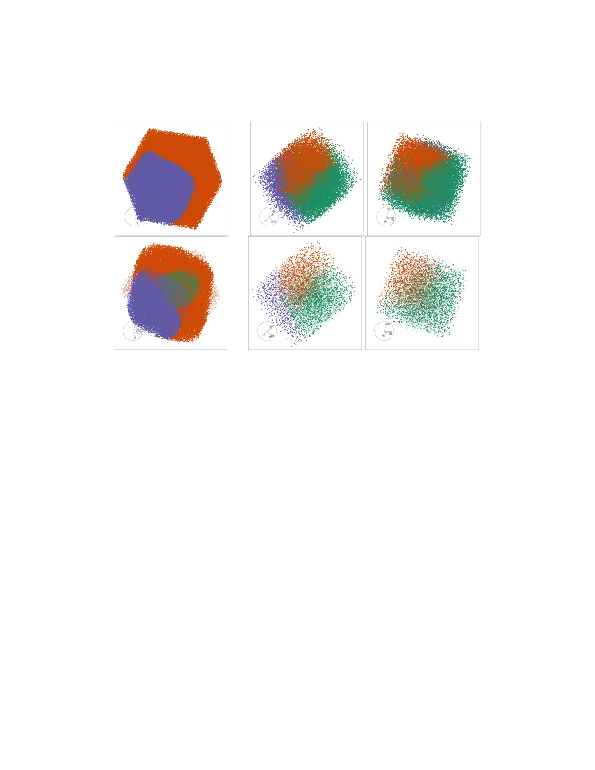
A slice tour for finding hollo wness in high-dimensional data Ursula Laa 1,2 , Dianne Co ok 2 , and German V alencia 1 1 Sc ho ol of Physics and Astronom y , Monash Univ ersit y 2 Departmen t of Econometrics and Business Statistics, Monash Univ ersity Octob er 25, 2019 Abstract T aking pro jections of high-dimensional data is a common analyt- ical and visualisation technique in statistics for w orking with high- dimensional problems. Sectioning, or slicing, through high dimensions is less common, but can b e useful for visualising data with conca vities, or non-linear structure. It is asso ciated with conditional distributions in statistics, and also link ed brushing betw een plots in in teractive data visualisation. This short tec hnical note describ es a simple approac h for slicing in the orthogonal space of pro jections obtained when run- ning a tour, thus presen ting the view er with an in terp olated sequence of sliced pro jections. The metho d has b een implemented in R as an extension to the tourr pack age, and can b e used to explore for conca ve and non-linear structures in multiv ariate distributions. Keyw ords: data visualisation; grand tour; sectioning; statistical com- puting; statistical graphics; high-dimensional data 1 In tro duction Data is commonly high-dimensional, and visualisation often relies on some form of dimension reduction. This can b e done by taking linear pro jections, 1 or nonlinear if one considers tec hniques like multidimensional scaling (MDS) (Krusk al and Wish 1978) or t-Distributed Sto c hastic Neighbour Em b edding (t-SNE) (v an der Maaten and Hinton 2008). F or the purp oses here, the fo cus is on linear pro jections, in particular as provided by the grand tour (Asimo v 1985; Buja et al. 2005). Interactiv e and dynamic displays can pro- vide information b eyond what can b e ac hiev ed in a static display . The grand tour sho ws a smooth sequence of in terp olated lo w dimensional pro jections, and allo ws the viewer to extrap olate from the low-dimensional shap es to the m ultidimensional distribution. It is particularly useful for detecting clusters, outliers and non-linear dep endence. A ma jor limitation of pro jections is their opacit y . It is mitigated some, when scatterplots are used to render the pro jected data, through a pseudo- transparency of sparseness of p oints. This is improv ed further if p oints are also drawn using an alpha level that pro vides transparent dots on most dis- pla y devices. Some features of m ultiv ariate distributions may b e visible, but a lot is easily hidden, esp ecially in the case of concav e structures. Consid- ering the example of a simple geometric shape suc h as a hypershere, it is difficult to distinguish betw een a full or a hollow sphere, that is, whether p oin ts are uniformly distributed within the sphere or on the surface of a sphere. Similarly we can think of small scale structures hidden in the cen tre of a multiv ariate distribution, that might b e considered to b e “needles in a ha ystack”, which can b e difficult to detect in pro jections. Pro jections also obscure non-linear b oundaries as migh t b e constructed from a classification mo del, or nonlinear mo del fits in high-dimensions. Slicing, or sectioning, is a wa y that the in ternal distribution of high- dimensional data can b e explored. F urnas and Buja (1994) discusses a tech- nique for combining pro jections with sections constructed by slicing in the dimensions orthogonal to the pro jection. It is also p ossible to think of linked brushing (e.g. Swa yne et al. (2003), O’Connell, Hurley , and Domijan (2017)) as slicing. In this note, w e discuss an approach to sectioning, where obser- v ations in the space orthogonal to the pro jection are highlighted if they are close to a pro jection plane through the mean of the data, and faded if fur- ther afield. This is com bined with the grand tour to pro vide a new dynamic displa y that can b e used to systematically searc h for features hidden in high dimensions. The new section tour metho d is describ ed in Section 2, and it is imple- men ted in the tourr (Wickham et al. 2011) pack age in R (R Core T eam 2018) (Section 3). Section 4 illustrates the use on several high-dimensional 2 geometric shap es and established data sets, sho wing ho w conca v e or o ccluded structures can b e visualised and explored with a slice tour. F uture work is discussed in Section 5. 2 Metho d 2.1 T our review A tour pro vides a con tinuous sequence of d -dimensional (t ypically d = 1 or 2) pro jections from p -dimensional Euclidean space. It is constructed by com bining a metho d for basis selection with geo desic in terp olation b etw een pairs of bases. In a grand tour, the basis selection is random, each new basis is c hosen from all p ossible pro jections. In a guided tour, the bases are chosen based on an index of interestingness. Differen t basis selection metho ds as well as the geo desic in terp olation are implemented in the tourr pac k age (Wickham et al. 2011), whic h also provides sev eral display functions for viewing the tour. F or the explanation of the slice tour, the actual mechanics of the tour are not imp ortant, and only the notion of a pro jection plane in high dimensions is needed. The notation used for explanations starts with denoting eac h pro jec- tion as X the n × p dimensional data matrix ( n observ ations in p dimensions) and A an orthonormal p × d pro jection matrix. The d -dimensional pro jection of the data is thus given by Y = X · A , pro ducing the n × d dimensional pro jected data matrix to b e plotted in each frame of the tour display . T o mak e a section, w e are in terested in the orthogonal distance of the data p oin ts from a pro jection plane, particularly using d = 2, but the approac h theoretically w orks for any d . 2.2 Slicing in the orthogonal space 2.2.1 Distance from the origin The orthogonal distance of the data p oints from the curren t pro jection plane is calculated as, ˜ v 2 i = || x 0 i || 2 , (1) 3 where x 0 i = x i − ( x i · a 1 ) a 1 − ( x i · a 2 ) a 2 (2) and x i , i = 1 , ..., n is a p -dimensional observ ation in X and a k , k = 1 , 2(= d ) denoting the columns of the pro jection matrix, A = ( a 1 , a 2 ). A is assumed to b e through 0, b ecause the data has b een cen tred on its mean. x 0 i can b e considered to b e a normal from the pro jection plane to x i , and then the norm of this v ector giv es the orthogonal distance b et w een p oin t and plane. This can b e generalized for d > 2. The distance can then b e used to display a slice tour b y highlighting points for whic h the orthogonal distance is smaller than a selected cutoff v alue h . In 3D, where for eac h plane there is only a single orthogonal direction, this defines a flat slice of height 2 h . W e could use this single direction to slice systematically from one side of the space to the other. It is also p ossible to think of fron t and bac k, some p oin ts are closer to the view er, and some are far, and depth cues could b e used. When going b ey ond 3D, the dimension of the orthogonal space is > 1, and all sense of direction is lost. In general, there are ( p − d ) dimensions orthogonal to the pro jection plane, and using distance from the p oints to the plane is the simplest approach to generating slices. Using the Euclidean distance results in rotation inv ariant slicing in the orthogonal space, where a “slice” is spherical in the orthogonal subspace, and has radius h . Figure 1 sho ws slices through 4D solid and hollow geometric shap es. F or eac h shap e, the p oin ts are generated either uniformly within the shap e, or on the surface. This illustrates the ease of distinguishing the solid from the hollo w, once slices are made. Figure 2 illustrates the slicing metho d for 3D and higher dimensions. 2.2.2 Slice thic kness Cho osing the slice thickness is a compromise b etw een what feature size can b e resolved and the sparseness of the data. As p increases, the relative n umber of points that are inside a slice of fixed thic kness h will decrease. The exact relation dep ends on the distribution of the data p oints. T o get a b est estimate for h , giv en p , assume that the points are uniformly distributed in a hypersphere. This is a rotation in v ariant uniform distribution in p space, and b ecause with slicing we are mostly interested in hollowness this is more relev an t than assuming a multiv ariate normal distribution. 4 The fraction of p oin ts inside a slice of thickness h can b e estimated as the relativ e v olume of the slice compared to the v olume of the full hypersphere, V rel = 1 2 h p − 2 R p ( pR 2 − ( p − 2) h 2 ) ≈ 1 2 ( h R ) p − 2 , (3) where R is the radius of the h yp ersphere. The appro ximation is v alid when h  R , as is typically exp ected to b e the case. T o keep the relative num b er of p oints (i.e. V rel ) approximately constant for slices in different dimensions p , we calculate h from a volume parameter as h =  1 / ( p − 2) , where  is a pre-c hosen v alue indicating a fraction of the ov erall v olume to slice, say 0.1. 2.2.3 Non-cen tral slice The equations abov e assume that the pro jection plane, and thus the the slice, passes through 0, whic h will be the mean of cen tred data. This (cen tre p oin t) is generally a go od option for the slice tour, because as the tour progresses the pro jection plane c hanges and can catch non-cen tral conca vities, too. How ever it is straigh tforward to generalize the equations to use any centre p oin t, c . In general c can b e any p oint in the p -dimensional parameter space, but w e are only in terested in the orthogonal comp onen t, the part of the v ector extending out of the pro jection plane, c 0 = c − ( c · a 1 ) a 1 − ( c · a 2 ) a 2 . The generalized measure of orthogonal distance is then v 2 i = || x 0 i − c 0 || 2 = x 0 2 i + c 0 2 − 2 x 0 i · c 0 (4) where the cross term can b e expressed as x 0 i · c 0 = x i · c − ( c · a 1 )( x i · a 1 ) − ( c · a 2 )( x i · a 2 ) . (5) Using the generalized distance measure with a cutoff volume,  , then corresp onds to moving a slice of fixed thickness, corresp onding to a neigh- b ourhoo d of the pro jection plane through the cen tre point c . In 3D, this simply corresponds to mo ving up or down along the orthogonal direction. Note that mo ving c off-centre will result in few er p oints inside a s lice for most data. 3 Implemen tation The slice tour has b een implemen ted in R (R Core T eam 2018) as a new displa y metho d display slice in the tourr pack age (Wickham et al. 2011). 5 a b c d Figure 1: Sliced pro jections through 4D geometric shap es. On the left a full (hollo w) h yp ersphere (a, b), on the righ t a full (hollo w) h yp ercub e (c, d). P oints inside the slice are sho wn as blac k bullets, p oin ts outside the slice are sho wn as grey dots. W e can clearly distinguish the full from the hollow ob jects based on the slice display . In addition to usual parameters the user can choose the volume parameter  b y setting eps and, if required, the cen tre p oin t c is set b y the anchor argumen t. By default eps=0.1 and anchor=NULL , resulting in slicing through the mean. In addition the user can select the marker sym b ols for p oin t inside and outside the slice. By default p oin ts in the slice are highlighted as pch slice = 20 and pch other = 46 , i.e. plotting a bullet for p oints inside the slice, and a dot for p oin ts outside. Belo w we sho w example co de for displa ying slices through a hollow 3D sphere. library (tourr) # use geozoo to generate points on a hollow 3D sphere sphere3 <- geozoo :: sphere.hollow ( 3 ) $ points colnames (sphere3) <- c ( "x1" , "x2" , "x3" ) # naming variables # slice tour animation with default settings animate_slice (sphere3) # trying an off-center anchor point, thicker slice, and # we use pch=26 to hide points outside the slice anchor3 <- rep ( 0.7 , 3 ) animate_slice (sphere3, anchor = anchor3, eps = 0.2 , pch_other= 26 ) 6 o c c’ A h  1 o A x x || x ⊥ Figure 2: Illustrations of slicing, through a 3D sphere (left), and demonstrat- ing the calculation of the orthogonal distance (right). 3D slicing can b e done b y sliding the pro jection plane along the orthogonal direction: centred at the origin (green) and one off-cen tre at c (blue). This intuition do es not transfer to higher dimensions, and it is b est to use orthogonal distance b etw een p oint and pro jection plane for computing the slice. Because a pro jection plane has no specific lo cation, for slicing w e can prescribe this, as through the data cen tre, or any other p oint, c . 4 Examples 4.1 Geometric shap es Using the geozoo pac k age (Sc hlo erke 2016) a num b er of ideal shap es are generated. 4.1.1 Hollo w sphere W e sample points on the surface of a sphere with radius R = 1 in p = 3 and p = 5 dimensions. Using the sphere.hollow() function, w e generate t wo sample data sets by generating 2000 and 5000 p oin ts from a uniform distribution on the surface of a 3D and 5D spheres. F or b oth examples w e start b y slicing through the origin with the default parameters, in particular  = 0 . 1, i.e. h = 0 . 1 in 3D and h = 0 . 46 in 5D. Slicing through the origin results in sections where the p oints inside the slice are appro ximately on a circle with the full radius, and eac h view is similar to that shown in Figure 1. It is especially instructive to look at spheres that are sliced off-cen tre. In this case the differen t views obtained in the slice tour reveal more of 7 the concav e structure of the distribution. The first ro w of Figure 3 sho ws example views from a slice tour on a 3D sphere with R = 1 and cen tre p oin t (0 . 7 , 0 . 7 , 0 . 7). Notice that this was c hosen to fall outside the sphere. Dep ending on the viewing angle selected b y the tour the slice con tains p oin ts on the circle with radius R (when the centre p oin t has a negligible orthogonal comp onen t to the viewing plane); a circle with radius < R as the viewing angle is tilted aw ay from the axis connecting the centre p oin t to the origin; a full circle with small radius as the angle increases; and finally we see an empt y slice when the pro jection plane is orthogonal to the centre p oin t axis. A similar picture is found for the 5D sphere, see second ro w of Figure 3. F or this example we generate 20k p oints on a hollo w 5D sphere to resolve the features. Since h increases with p the resolution is reduced compared to the 3D example. Note also that as dimensionalit y increases, the larger orthogonal space means that the centre p oint will ha ve a large orthogonal comp onen t in most views. Figure 3: Different slices through a 3D (first ro w) and 5D (second ro w) hollo w sphere with R = 1, with shifted centre p oint, showing full circle with small radius (left), circle with radius < R (middle) and circle with radius R (righ t). 4.1.2 Other geometric shap es T o better understand the slice tour w e lo ok at differen t examples of geometric shap es, see Figure 4. F or each shap e tw o selected views are sho wn. The first column sho ws views from the slice tour on a 3D Roman surface. The second column sho ws slices through a 4D torus, revealing different asp ects of the 8 shap e. The last column sho ws a 6d cub e, where the upp er plot sho ws a view along tw o of the original parameters, allo wing to clearly iden tify the rectangular shap e. The panel b elo w shows that this is not typically the case when lo oking at a randomly selected slice. Figure 4: Differen t slices through a Roman surface (left), 4D torus (middle) and a 6d cub e (right). 4.2 Other examples 4.2.1 Needle in a haystac k W e use the p ollen data as an example for a hidden feature generally o ccluded in pro jections. This is a classic 5D data set, originally simulated by David Coleman of R CA Labs, for the Joint Statistics Meetings 1986 Data Expo (Coleman 1986). The standardised data is observ ed in a slice tour with a thin slice (  = 0 . 0005). Selected views are shown in the first tw o plots in Figure 5. They indicate the presence of an interesting feature hidden in the cen tre, which can b e identified as the w ord “EUREKA” b y zo oming. 4.2.2 Non-linear b oundaries Wic kham, Co ok, and Hofmann (2015) describ ed some principles and ap- proac hes for visualising mo dels in the data space. Much of this is based on ex- amining pro jections provided by a tour of the mo del in the high-dimensional 9 Figure 5: Differen t slices through the classic p ollen dataset. The first tw o plots hav e slice v olume  = 0 . 0005, the last t w o plots zo om in on the centre and hav e increased v olume  = 0 . 005. The hidden w ord can b e seen in the zo omed slice. space. Classification b oundaries are explored for the wine data set (Asun- cion and Newman 2007). It is difficult to digest the b oundaries fully – for example, where one group’s b oundary wraps another, if they are linear or nonlinear, or whether the boundary go es through the space or is only carving out a corner of it. The sliced pro jections makes this easier. Selected views of pro jections and sliced pro jections from a radial basis SVM on 3 v ariables, and a p olynomial basis SVM on 5 v ariables are shown in Figure 6. The slicing allows exploring the cen tre of the space. With 3D it rev eals the spherical boundary of the group (green) hidden b y the pro jection. In 5D with the polynomial basis, pro jection migh t suggest that the boundary b et ween classes is almost linear, but the slicing shows that it to b e nonlinear near the cen tre. 5 Discussion This pap er has in tro duced a new visualization metho d for dynamic slicing of high-dimensional spaces. It is based on interpolated pro jections obtained in a (grand) tour and generates an in terp olated sequence of sliced pro jec- tions. The examples sho wn in Section 4 demonstrate the potential of this new display to find and explore concav e structures, as well as other hidden features. A default slice thickness is provided with the algorithm, that takes di- mensionalit y into account. As the data dimension increases, more p oin ts in the sample are needed, and a thick er slice ma y b e needed. Generally , the tour can b e slow to view when there are a large num b er of samples, and the slicing, where only p oints inside the slice are drawn, might also b e a w a y to 10 Figure 6: Exploring classification b oundaries of the wine dataset using pro- jection (top ro w) and sliced pro jection (bottom r o w). Radial basis SVM (first column) of 3 v ariables sho ws ho w the slicing rev eals the spherical shape of the b oundary of one group (green) that was hidden in the pro jection. Polyno- mial basis SVM (second and third columns) of 5 v ariables. The orange group do es tend to b e wrapp ed by the green group, and the blue group disapp ears with slicing, sho wing that it is on the outer edge of the space. impro ve the display drawing, with a fo cus on the imp ortan t features. Sliced 2D tours w ere a v ailable in XGobi (Swa yne, Co ok, and Buja 1998) but w ere not do cumented. This w ork makes them av ailable in the tourr pac k age. It is a simple, but effective, approach to taking slices. The approach b y F urnas and Buja (1994) is more complex, and slices a subspace of the p − d = p − 2 dimensional space orthogonal to the pro jection. This generates a more parameters, making it more difficult to navigate. More parameters mean more decisions on what to show. Ho wev er, it is one of the next steps to explore differen t definitions of a slice tour, and the types of structure that migh t b e captured by v ariations in slicing algorithms. Lastly , there is a large literature on pro jection pursuit, and some of this w ork is av ailable in the pro jection pursuit guided tour in the tourr pack age. 11 The pro jections shown are more in teresting in a guided tour than might b e seen using a grand tour. The slicing migh t be in tro duced in to pro jection pur- suit by defining weigh ted pro jection pursuit indexes. The resulting indexes could b e incorp orated into a guided slice tour, finding pro jections where the slice rev eals something new. 6 Ac kno wledgemen ts The authors gratefully ackno wledge the supp ort of the Australian Research Council. The pap er was written in rmarkdown (Xie, Allaire, and Grolemund 2018) using knitr (Xie 2015). The source material and animated gifs for this pap er are av ailable at https://github.com/uschiLaa/paper- slice- tour . An app endix deriving the relativ e slice volume for the h yp ersphere is included as supplemen tal material. References Asimo v, D. 1985. “The Grand Tour: A To ol for Viewing Multidimensional Data.” SIAM Journal of Scientific and Statistic al Computing 6 (1): 128–143. Asuncion, A., and D.J. Newman. 2007. “UCI Machine Learning Rep ository .” http:// www.ics.uci.edu/ ~ mlearn/MLRepository.html . Buja, A., D. Co ok, D. Asimov, and C. Hurley . 2005. “Computational Metho ds for High- Dimensional Rotations in Data Visualization.” 391–413. Coleman, David. 1986. “Geometric F eatures of Pollen Grains.” http://lib.stat.cmu. edu/data- expo/ . F urnas, George W., and Andreas Buja. 1994. “Prosection Views: Dimensional Inference through Sections and Pro jections.” Journal of Computational and Gr aphic al Statistics 3 (4): 323–353. http://www.jstor.org/stable/1390897 . Krusk al, J.B., and M. Wish. 1978. “Multidimensional Scaling.” Sage University Pap er Series on Quantitative Applic ations in the So cial Scienc es No. 07-011. O’Connell, Mark, Catherine Hurley , and Katarina Domijan. 2017. “Conditional Visualiza- tion for Statistical Mo dels: An Introduction to the condvis Pac k age in R.” Journal of Statistic al Softwar e, Articles 81 (5): 1–20. https://www.jstatsoft.org/v081/i05 . R Core T eam. 2018. R: A L anguage and Envir onment for Statistic al Computing . Vienna, Austria: R F oundation for Statistical Computing. https://www.R- project.org/ . 12 Sc hlo erk e, Barret. 2016. ge ozo o: Zo o of Ge ometric Obje cts . R pac k age version 0.5.1, https: //CRAN.R- project.org/package=geozoo . Sw a yne, D. F., D. Co ok, and A. Buja. 1998. “XGobi: Interactiv e Dynamic Graphics in the X Window System.” Journal of Computational and Gr aphic al Statistics 7 (1): 113–130. Sw a yne, Deb orah F., Duncan T emple Lang, Andreas Buja, and Dianne Co ok. 2003. “GGobi: evolving from XGobi into an extensible framework for interactiv e data vi- sualization.” Computational Statistics & Data Analysis 43: 423–444. v an der Maaten, L., and G. Hinton. 2008. “Visualizing Data using t-SNE.” Journal of Machine L e arning R ese ar ch 9: 2579–2605. Wic kham, Hadley , Dianne Cook, and Heik e Hofmann. 2015. “Visualizing statistical mo d- els: Remo ving the blindfold.” Statistic al Analysis and Data Mining: The ASA Data Scienc e Journal 8 (4): 203–225. https://onlinelibrary.wiley.com/doi/abs/10. 1002/sam.11271 . Wic kham, Hadley , Dianne Co ok, Heike Hofmann, and Andreas Buja. 2011. “tourr: An R Pac k age for Exploring Multiv ariate Data with Pro jections.” Journal of Statistic al Softwar e 40 (2): 1–18. http://www.jstatsoft.org/v40/i02/ . Xie, Yihui. 2015. Dynamic Do cuments with R and knitr . 2nd ed. Bo ca Raton, Florida: Chapman and Hall/CR C. https://yihui.name/knitr/ . Xie, Yihui, Joseph J. Allaire, and Garrett Grolemund. 2018. R Markdown: The Definitive Guide . Chapman and Hall/CR C. https://bookdown.org/yihui/rmarkdown . 13