Sparse Representation-based Image Quality Assessment

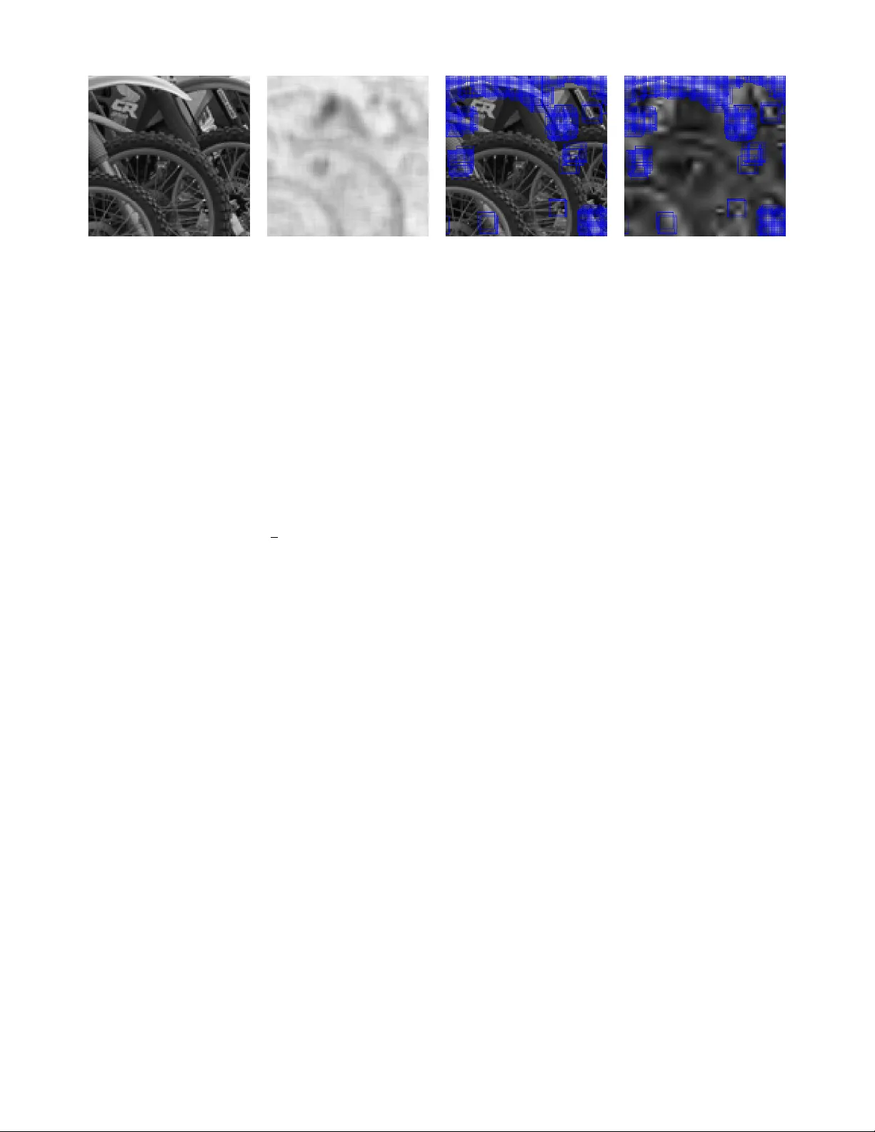
JOURNAL OF L A T E X CLASS FILES, VOL. 6, NO. 1, J ANU AR Y 2007 1 Sparse Representation-based Image Quality Assessment T anaya Guha, Student Member , IEEE, Ehsan Nezhadarya, Student Member , IEEE, and Rabab K W ard, F ellow , IEEE Abstract —A successful approach to image quality assessment in volves comparing the structural information between a dis- torted and its refer ence image. However , extracting structural information that is per ceptually important to our visual system is a challenging task. This paper addresses this issue by employing a sparse repr esentation-based approach and proposes a new metric called the sparse representation-based quality (SP ARQ) index . The proposed method learns the inherent structur es of the refer ence image as a set of basis vectors, such that any structure in the image can be r epresented by a linear combination of only a few of those basis vectors. This sparse strategy is employed because it is known to generate basis vectors that are qualitatively similar to the recepti ve field of the simple cells present in the mammalian primary visual cortex [1]. The visual quality of the distorted image is estimated by comparing the structures of the r eference and the distorted images in terms of the learnt basis vectors resembling cortical cells. Our approach is ev aluated on six publicly av ailable subject-rated image quality assessment datasets. The proposed SP ARQ index consistently exhibits high corr elation with the subjective ratings on all datasets and perf orms better or at par with the state-of- the-art. Index T erms —Dictionary learning, Image quality , sparse rep- resentation, structural similarity . I . I N T R O D U C TI O N D IGIT AL images incur a v ariety of distortions during the process of image acquisition, compression, transmission, storage or reconstruction. These often degrade the visual quality of images. In order to monitor, control and improve the quality of images produced at the various stages, it is important to automatically quantify the image quality . Since the end-users of the majority of image-based applications are humans, this requires the understanding of human perception of image quality , and mimicking it as closely as possible. The mean squar ed error (MSE) and the peak signal-to- noise ratio (PSNR) hav e been traditionally used to measure the image quality degradations. These metrics, although math- ematically con venient, f ail to correlate well with human per - ception [2]. A considerable amount of research effort has been put towards quantifying the quality of images as percei ved by humans, and a number of objective image quality assessment algorithms that agree with the subjecti ve judgment of human beings hav e been developed. The objective quality assessment methods, depending on whether or not they use some or all the information about the original undistorted image, are The authors are with the Image and Signal Processing Lab, department of Electrical and Computer Engineering, the University of British Columbia, V ancouver , BC, Canada. email: { tanaya, ehsann, rababw } @ece.ubc.ca broadly classified into three categories: no-refer ence , r educed- r efer ence and full-r eference [3]. This paper concentrates on the full-reference quality estimation approach. The earlier focus of full-reference image quality assess- ment research has been on building a comprehensive and accurate model of the human visual system (HVS) and its psychophysical properties, such as the contrast sensiti vity function. In this approach, the errors between the distorted and the reference images are quantized and pooled according to the HVS properties [4]. These methods require precise knowledge of the viewing conditions and are computationally demanding. Despite this complexity , the HVS modeling-based methods can only mak e linear or quasilinear approximations of the highly non-linear HVS. Our current understanding of the HVS is also limited in many aspects. Consequently , these methods are not highly superior to MSE or PSNR [5]. The interest of modern image quality estimation research lies in modeling the content of the images based on cer- tain significant properties of the HVS. This visual fidelity- based approach is more attractiv e because of its practicality and mathematical foundation [6], [7]. The majority of these fidelity-based methods attempt to quantify the perceptual qual- ity either in terms of statistical information [8], [9] or in terms of structural information of the images [5], [10]–[14]. The statistical approaches hypothesize that the HVS has ev olved ov er the years to extract information from natural scenes and therefore, use natural scene statistics to estimate the perceptual quality of images. The structural approaches on the other hand operate on the basis of a rather important aspect of the HVS - its sensitivity towards the image structures for dev eloping cognitiv e understanding. In this approach, image quality is estimated in terms of the fidelity of structures between the reference and the distorted images. The representative image quality metric of the class of structural information-based metrics is the structural similarity index (SSIM) [10]. SSIM treats the non-structural distortions (such as, luminance and contrast change) separately from the structural distortions. The quality of a patch in the distorted image is measured by comparing it with the corresponding patch in the original image in terms of three components: luminance, contrast and structure. A global quality score is computed by combining the effects of the three compo- nents ov er all image patches. SSIM achiev ed much success because of its simplicity , and its ability to tackle a wide variety of distortions. Due to its pixel-domain implementa- tion, SSIM is highly sensitive to geometric distortions like scaling, translation, rotation and other misalignments [4]. T o JOURNAL OF L A T E X CLASS FILES, VOL. 6, NO. 1, J ANU AR Y 2007 2 Fig. 1. Overview of the proposed image quality assessment approach improv e the performance of SSIM, multiscale extension [11], wa velet transform-based modification [14], gradient-domain implementation [12] and various pooling strategies [13], [15] hav e been proposed. The underlying assumption behind utilizing the structural information is that the HVS uses the structures extracted from the vie wing field for its cogniti ve understanding. Therefore, a high-quality image is expected to preserve all the structural information of the reference image. From this vie wpoint, efficiently capturing the structural information of images is the key to developing successful image quality assessment algorithms. But extracting the structural information in a perceptually meaningful way is a non-trivial task. A widely used mathematical tool for analyzing image structures is the wa velet transform. Its basis elements, being spatially localized, oriented and of bandpass in nature, resemble the receptiv e field of simple cells in the mammalian primary visual cortex (also known as the striate cortex and V1) [1], [4]. Howe ver , the wa velet transform uses a set of predefined, data-independent basis functions - the success of which is often limited by the degree as to how suitable they are in capturing the structure of the signals under consideration. W e consider a more generalized approach to analyzing signal structures. This in volv es learning a set of basis elements that are adapted to represent the inherent structures of the signal in question. These learnt basis elements are collectiv ely known as a dictionary . Such learning can be accomplished by fitting a set of basis vectors to a collection of training samples. As each basis vector is tailored to represent a significant part of the structures present in the given data, a learnt dictionary is more ef ficient in capturing the structural information compared to a predefined set of bases. More importantly , this approach empowers us to build a cortex-lik e r epresentation of an image. In 1996, Olshausen and Field hav e sho wn that basis elements that r esemble the pr operties of the r eceptive field of simple cells in the primary visual cortex can be learnt fr om the input images [1]. They showed that the keys to building such a cortex-like dictionary are: (i) a sparsity prior - an assumption that it is possible to describe the input image using a small number of basis elements, and (ii) over completeness - the number of basis elements in the dictionary is greater than the vector space spanned by the input. Until recently , this important result was not exploited to its full strength in the field of signal or image processing. In the last few years, se veral practical dictionary learning algorithms ha ve been dev eloped [16], [17]. It has been shown that the data-dependent, learnt dictionaries, due to their superior ability to model the inherent structures in the data, can outperform predefined dictionaries like wav elets in several image processing tasks [16], [18], [19]. In this paper, we de velop a full-reference image quality assessment metric which we name the spar se r epr esentation- based quality (SP ARQ) index . The metric relies on capturing the inherent structures of the reference image in a perceptually meaningful way . T o achiev e this, an o vercomplete dictionary and its corresponding sparse representation are learnt from local patches of the image. The local structures in the distorted image are decomposed using the basis vectors of the learnt dictionary and the resulting sparse coef ficients are used to quantify the perceptual quality of the distorted image with respect to the reference image. As our method analyzes the image structures by building a cortex-like model of the stim- uli, the extracted information is expected to be perceptually meaningful. This is much different from existing structural information-based methods which, although successful, pro- vide no e vidence on the perceptual importance of the structural information they extract from images. T o ev aluate the efficac y of the proposed metric, we perform various experiments on six publicly a vailable, subject-rated image quality assessment datasets: LIVE [20], A57 [21], CSIQ [22], MICT [23] and WIQ [24]. The proposed SP ARQ index consistently exhibits JOURNAL OF L A T E X CLASS FILES, VOL. 6, NO. 1, J ANU AR Y 2007 3 high correlation with the subjectiv e scores and often outper- forms its competitors. The rest of the paper is organized as follo ws. Section II describes the proposed quality estimation approach, follo wed by the experimental results and discussions in Section III. Sec- tion IV concludes the article and suggests possible directions to future work. I I . T H E P R O P O S E D A P P RO AC H Our image quality assessment method is divided into two phases: a tr aining phase and a quality estimation phase. The goal of the training phase is to model the inherent structures of the reference image in a perceptually meaningful way . This is achiev ed by learning an ov ercomplete dictionary from the reference image. In the quality estimation phase, a quality score, namely the SP ARQ index, is computed by comparing the information in selected regions of the reference image with those in the distorted image. Figure 1 presents an ov erview of the proposed method, and the steps are described below in detail. A. T raining Phase This step in volv es learning (i) a dictionary i.e. set of basis vectors whose properties resemble those of the receptiv e field of simple cells in primary visual cortex, and (ii) the weights by which these basis elements are mixed together . 1) Motivation behind learning a cortex-lik e dictionary: The motiv ation of this approach comes from the very process of image formation and how is it perceived by the HVS. The nat- ural viewing field is highly structured and spatially correlated. The light rays that reflect off various structures in the viewing field, get focused onto an array of photoreceptors present in the retina. The information is then encoded in the form of complex statistical dependencies among the photoreceptor activities [25]. The goal of primary visual cortex, as indicated in se veral seminal studies [1], [25], is to reduce these statistical dependencies in order to discov er the intrinsic structures that gav e rise to the image. A reasonable strategy towards mimicking this phenomena is to describe an image in terms of a linear superposition of a few basis vectors. These basis vectors form a subset of an ov ercomplete set of basis vectors (dictionary) that are adapted to the given image so as to best represent the structures in the images [1], [25]. It has been shown that on employment of this strategy , the basis elements that emerge are qualitati vely similar to the receptiv e field of the cortical simple cells [1]. The conjecture that sparsity is an important prior is based on the observation that natural images contain sparse structures and can be described by a small number of structural primitiv es like lines and edges [25], [26]. Due to ov ercompleteness, the basis vectors are also non-orthogonal and the input-output relationship deviates from being purely linear . The justification of de viating from a strictly linear approach is to account for a weak form of nonlinearity exhibited by the simple cells themselves [25]. 2) Learning a dictionary: Given a reference image, I ref ∈ R N , we intend to learn an overcomplete dictionary . This can be achie ved by fitting the basis vectors in the dictionary to represent the local structures of the image. T o account for the local structures in an image, a large number of distinct, possibly overlapping patches of dimension √ n × √ n are extracted randomly from I ref . Ideally , one patch centerd at e very pixel should be extracted; but in practice, extracting any large number of patches is sufficient for learning a good dictionary . After extracting a large number of random patches, the patches with lo w or no structural information i.e. the homogeneous patches are discarded. This is done by removing the patches whose variance is zero or close to zero after mean removal. A number of k patches are then selected from the set of the informativ e patches. Each image patch is con verted to a vector of length n . These patches are concatenated to form a matrix P ∈ R n × k where k is the number of patches extracted from I ref and the columns of P are the patch vectors. From these patches, a dictionary Φ = { φ i } m i =1 , φ i ∈ R n is learnt. W e are interested in the over complete case where n < m i.e. when Φ has more basis vectors than the dimensionality of the input. An o vercomplete dictionary offers greater flexibility in representing the essential structures in a signal. It is also robust to additi ve noise, occlusion and small translation [27]. Howe ver , greater difficulties arise with overcompleteness, because a full-rank, overcomplete Φ creates an underdeter- mined system of linear equations having an infinite number of solutions. T o narro w down the choice to one well-defined solution, an additional constraint of sparsity is enforced. Let, the sparse representation of P ov er the dictionary Φ be denoted by X = { x i } k i =1 , x i ∈ R m where any patch vector in P can be represented by a linear superposition of no more than τ dictionary columns where τ << m . This is formally written as the follo wing optimization problem: min { Φ , X } n k P − ΦX k 2 F o sub ject to k x k 0 ≤ τ (1) where k . k F is the Frobenius norm (square root of the sum of the squared v alues of all elements in a matrix) and k . k 0 is the ` 0 semi-norm that counts the number of non-zero elements in a vector . Although the ` 0 norm provides a straightforward notion of sparsity , it renders the problem non-con vex. Thus obtaining an accurate solution of (1) is NP hard. Nevertheless, in the last few years researchers hav e found practical and stable ways to solve such underdetermined systems via con vex optimization [28] and greedy pursuit algorithms [29]. T o solve (1), a recently de veloped learning algorithm, known as the K-SVD [16] is employed. K-SVD iterativ ely solves (1) by performing two steps at each iteration: (i) sparse coding and (ii) dictionary update. In the sparse coding step, Φ is kept fixed and the coefficients in X are computed by a greedy algorithm called the orthogonal matching pursuit (OMP) [29]. min X n k P − ΦX k 2 F o sub ject to k x k 0 ≤ τ (2) In the dictionary update step, each basis element φ i ∈ Φ is updated sequentially , allowing the corresponding coefficients JOURNAL OF L A T E X CLASS FILES, VOL. 6, NO. 1, J ANU AR Y 2007 4 in X to change as well. Updating an element φ i in volv es computing a rank-one approximation of a residual matrix E i . E i = f Y i − f Φ i f X i (3) where f Φ i and f X i are formed by removing the i -th column from Φ and the i -th row from X , and f Y i contains only those columns of Y that use φ i for their approximation. The rank- one approximation is computed by subjecting E i to a Singular V alue Decomposition (SVD). For the details of this learning algorithm, please refer to the original K-SVD paper [16]. B. The Quality Estimation Phase This part of our method first compares the reference and the distorted images locally , and then yields a global value as the measure of perceptual quality of the distorted image. This is accomplished through the follo wing steps: 1) Detection of salient patches: It is well-known that not ev ery pixel (or region) in an image receives the same lev el of visual attention. Sev eral studies have shown that significant improv ement in performance of the quality metrics can be achiev ed by incorporating information about visual attention i.e. by detecting perceptually important regions [30]–[32]. A common hypothesis is that the HVS is an efficient extrac- tor of information, and therefore the image re gions that contain high information attract more visual attention [13], [15]. Based on this hypothesis, we take an information theoretic approach tow ards detecting the visually important regions or patches. One way to quantify the local information content of an image is by computing the Shannon’ s entropy of each patch. The information content or entropy of a discrete random variable z with probability distrib ution P z = { p 1 , p 2 , ..., p J } is defined as H ( z ) = H ( P z ) = − J X j =1 p j log 2 p j (4) Similarly , an image patch can also be analyzed as a random variable. Let us consider an image patch z of dimension √ n × √ n where each pixel in z is independent and identically distributed. If z contains J distinct intensity v alues, its proba- bility distribution, P z , is giv en by P z = { p 1 , p 2 , ..., p J } , where J ≤ 2 8 for an 8-bit grayscale image; p j is the probability of the pixel intensity v alue j . The probability p j is defined as p j = f j /n , where f j is the number of pixels (frequency) with intensity value j occurs in the image patch z and n is the total number of pixels in z . The entropy of ev ery √ n × √ n patch (a patch around e very pixel) in the reference image I ref ∈ R N is computed as H ( z ) = − J X j =1 p j log 2 p j = − 1 n J X j =1 f j log 2 ( f j /n ) (5) The lar ger the v alue of H , the higher is the information content of a patch. A number of q patches having the highest entropy values are selected as the salient patc hes in I ref . These patches are vectorized and arranged as columns of a matrix P r ∈ R n × q . The locations of these q patches are used to extract the corresponding patches from the distorted image I dis ∈ R N . The matrix containing the patches from the distorted image is denoted as P d ∈ R n × q . An example of this process is provided in Fig. 2 which shows a reference image, its local entropy map, the salient patches selected in the reference image and the corresponding patches selected in the distorted image. 2) Computation of the SP ARQ index: At this point, we hav e two sets of corresponding salient patches P r and P d extracted from the same locations of the reference and the distorted images. The next task is to analyze and compare these structures (patches) w .r .t. the previously learnt dictionary Φ . Let us consider a patch vector p r ∈ P r from I ref and its corresponding patch vector p d ∈ P d from I dis . The patches p r and p d are decomposed using Φ to obtain their respecti ve sparse coefficients x r and x d . min x r n k p r − Φx r k 2 2 o sub ject to k x r k 0 ≤ τ (6) min x d n k p d − Φx d k 2 2 o sub ject to k x d k 0 ≤ τ (7) Note that, each of x r and x d contains only τ non-zero elements. The locations (indices) of these non-zero coef ficients indicate those specific basis vectors in Φ which actually contribute to the approximation of the input patch. These activ e basis vectors are called the support of the input. The amplitudes of these non-zero coefficients are the weights by which these support vectors are combined. The support vectors and their weights together are indicati ve of the structural and non-structural distortions between the two input patches. Ideally , these two patches would have different sets of support vectors whene ver there exist any structural distortions between them. Otherwise, if the two patches undergo purely non- structural distortions, the supports would remain the same b ut their weights may change. In order to quantify the perceptual quality of p d w .r .t. p r , we compare their sparse representations x d and x r . A simple but ef fective way to compare two vectors is to compute their normalized correlation coefficient . A parameter α is computed based on the correlation coef ficient between x r and x d as follows: α ( p r , p d ) =   x T r x d   + c k x r k 2 k x d k 2 + c (8) where c is a small positiv e constant added to av oid instability when the denominator is close to zero. Clearly , 0 < α ≤ 1 . When x r and x d are orthogonal,   x T r x d   = 0 ; but due to the presence of c , the parameter α is slightly greater than zero. Due to normalization, α is unaffected by the lengths of x r and x d . Thus α is not be able to measure non-structural distortions caused by multiplying the patch elements by a constant. T o account for these types of distortions as well, we intro- duce another parameter . An important measure of similarity (or difference) between two vectors is their pointwise difference. Hence, we compute another quantity β which uses the length of the vector ( x r − x d ) . β ( p r , p d ) = 1 − k x r − x d k 2 + c k x r k 2 + k x d k 2 + c (9) JOURNAL OF L A T E X CLASS FILES, VOL. 6, NO. 1, J ANU AR Y 2007 5 (a) (b) (c) (d) Fig. 2. Detection of salient regions: (a) Reference image, (b) Local entropy map of the reference image (brighter pixel value indicates higher entropy), (c) Salient patches detected in the reference image based on the entropy map, and (d) Corresponding patches in the distorted image. The images are cropped at the middle for display (best viewed in color). where c is the same positi ve constant used in (8) . It is easy to see that 0 < β < 1 . W e propose a function S ( p r , p d ) that measures the percep- tual quality of p d w .r .t p r as follows: S ( p r , p d ) = α ( p r , p d ) β ( p r , p d ) (10) Let S ( p i r , p i d ) be the quality measure between the i th pair of salient patches i.e. ( p i r , p i d ) . The proposed global image quality SP ARQ( I ref , I dis ) is computed by averaging over all q salient patches. SP ARQ( I ref , I dis ) = 1 q q X i =1 S ( p i r , p i d ) (11) Remarks: • The SP ARQ index is bounded: 0 < SP ARQ < 1 ; it is always non-negati ve since each of its components is non- negati ve. • The highest value of SP ARQ is attained when I ref = I dis . • The index is not symmetric i.e. SP ARQ( I ref , I dis ) 6 = SP ARQ( I dis , I ref ) . This is because the dictionary Φ is trained on the reference image only . For the purpose of full-reference image quality assessment, where clear information about the reference image is av ailable, this is not an issue. Nev ertheless, symmetry can be easily achiev ed by repeating the quality estimation stage with a dictionary trained on the distorted image and av eraging the resulting quality scores obtained using the two dictio- naries. Our experiments sho w that this step has little or no significance on the performance of the SP ARQ inde x. I I I . E X P E R I M E N TA L V A L I DA T I O N This section presents a critical ev aluation of the proposed metric on six publicly av ailable image databases whose sub- jectiv e quality ratings are av ailable. These databases exhibit a variety of distortions such as compression artifacts, blurring, flicker noise, wireless artifacts, etc. The performance of an objectiv e quality assessment metric is ev aluated by comparing its results to the subjectiv e scores. Follo wing an e valuation methodology suggested by the video quality expert group (VQEG) [33], this comparison is made by computing corre- lation coefficients and differences between the subjecti ve and the objectiv e scores. The objecti ve scores of the SP ARQ index and those of six existing image quality assessment metrics are compared to the subjective ratings on each dataset. The six image quality assessment metrics are: PSNR, SSIM [10], PHVS-M [34], IFC [8], VIF [9], and VSNR [6]. The existing quality metrics are compared to the SP ARQ index on the basis of their closeness to the subjecti ve scores. The SP ARQ index consistently exhibits high correlation with the subjectiv e ratings on all datasets and performs better or at par with the state-of-the-art. A. The databases A brief description of each of the six datasets used in this work is provided below . The LIVE database [10], [20] contains 779 distorted images created from 29 original color images. Each distorted image exhibits one of the fiv e types of distortions: JPEG2000 com- pression (JP2K), JPEG compression (JPEG), additiv e white gaussian noise (A WGN), Gaussian blur and fastfading channel distortion of JPEG2000 compressed bitstreams. The Cornell-A57 dataset [6], [21] consists of 54 distorted images created from 3 original grayscale images. The im- ages are subject to the following 6 types of distortions: JPEG compression, JP2K compression, A WGN, Gaussian blur , JPEG2000 compression with dynamic contrast-based quanti- zation algorithm, and uniform quantization of LH subbands of a 5-lev el discrete wa velet transform at all scales. The CSIQ database [22] has 30 original images which were used to create 866 distorted images. The 6 distortion types (at four to fiv e distortion lev els) include JPEG compression, JP2K compression, global contrast decrements, A WGN, and Gaussian blurring. The TID database [35] is so far the largest subject-rated image dataset for quality ev aluation. It has 1700 images gener- ated from 25 reference images with 17 distortion types at four distortion lev els. The distortion types are: A WGN, additiv e noise in color components, spatially correlated noise, masked noise, high frequency noise, impulse noise, quantization noise, Gaussian blur, image denoising, JPEG compression, JP2K compression, JPEG transmission errors, JP2K transmission errors, non-eccentricity pattern noise, local block-wise distor - tions of different intensity , mean shift, and contrast change. JOURNAL OF L A T E X CLASS FILES, VOL. 6, NO. 1, J ANU AR Y 2007 6 Fig. 3. Performance of the SP ARQ index (correlation with subjecti ve scores measured in terms of SROCC) varies with the percentage of high-entropy patches used in the quality estimation process. The MICT -T oyoma database [23] contains 168 distorted images created from 14 reference images. The images exhibit 2 types of distortions: JPEG and JP2K compression. The WIQ database [24], [36] consists of 80 distorted im- ages generated from 7 reference images. The images exhibit wireless imaging artifacts which are not considered in other datasets. Due to the complex nature of a wireless communi- cation channel, the images contain more than one artifacts. B. P arameter settings Before computing the SP ARQ index, two preprocessing steps are ex ecuted: (1) ev ery color image in each dataset is con verted to grayscale image, and (2) each image is downsam- pled by a factor F so as to account for the vie wing condition. The v alue of F is obtained by using the follo wing empirical formula [10]. F = max(1 , round( g / 256)) (12) where g = min (#ro ws in I ref , #columns in I ref ) . The computation of the SP ARQ index is di vided into a training phase and a quality estimation phase. In the training phase, there are 4 parameters to be set: • √ n : the patch size • k : the number of patches to be extracted from a reference image for training the dictionary • m : the number of basis vectors in the dictionary • τ : the sparsity constraint Unfortunately , there is no theoretical guidelines to determine the values of these parameter , so we rely on pre vious work and empirical methods. A patch size of √ n × √ n = 11 × 11 is used following the patch-size specification of SSIM [10]. A collection of as large as k = 3000 patches are extracted randomly from e very reference image to train its correspond- ing dictionary . W e set the overcompleteness factor ( m/n ) to 2 which yields m = 242 . It has been shown that for low ov ercompleteness factor , sparse representations are stable in the presence of noise [37]. The value of τ is set to 12 which is approximately 10% of the dimensionality of the input vectors. In the quality estimation phase, we need 2 additional parameters: • c : the stabilizing constant in (8) and (9) • q : the number of salient patches The constant c is chosen to have a very small value, c = 0 . 01 , so as to ha ve minimal influence on the quality score. The value of q is determined empirically . For each database, the number of salient patches, q , is varied and the performance of SP ARQ is measured in terms of the correlation between its scores and the subjectiv e scores. This is presented in Fig. 3 where the Spearman’ s Rank Correlation Coef ficient (SR OCC) is plotted against q . The value of q is varied from 2% to 100% of N where N is the total number of patches (one around each pixel) in I ref or I dis . In fi ve out of the six datasets, the best performance of the SP ARQ index is observed when q = 0 . 15 N i.e. 15% of N . Also notice that, when all patches in I ref are used, the performance of the SP ARQ index degrades. This confirms our assumption that only the visually important areas are useful for quality assessment. For all datasets, we use the same parameter v alues. C. Evaluation methodology The results of an objective image quality assessment metric is compared with the subjecti ve scores using a set of e valuation measures suggested by the video quality expert group (VQEG) [33]. These ev aluation measures are - the Spearman’ s rank order correlation coefficient (SR OCC), the K endall’ s rank order correlation coefficient (KR OCC), the Pearson linear correlation coef ficient (CC), mean absolute error (MAE) and root mean squared error (RMS). The SR OCC and KROCC are used to measure the pr ediction monotonicity , while CC, MAE and RMS measure the pr ediction accuracy of the objectiv e scores. In order to compute CC, MAE and RMS, a five- parameter logistic function (refer to (13) and (14)) is fitted to the objectiv e scores. A particular objectiv e score, s , is mapped to a new score, Q ( s ) using a non-linear mapping function Q ( · ) which is defined as follo ws. Q ( s ) = γ 1 logistic( γ 2 , ( s − γ 3 )) + sγ 4 + γ 5 (13) logistic( σ, s ) = 1 2 − 1 1 + exp( σ, s ) (14) A MA TLAB function called fminunc is used for fitting. CC, MAE and RMS v alues are computed after the abo ve non-linear mapping between the subjective and objectiv e scores. Note that, SR OCC and KROCC are non-parametric rank correla- tion metrics and are independent of any nonlinear mapping between the subjectiv e and the objectiv e scores. For details of the ev aluation methodology please see [9], [13], [33]. A good image quality assessment metric is expected to hav e high SR OCC, KROCC and CC scores, and lo w MAE and RMS values. The performance of SP ARQ is compared with those of PSNR, SSIM, PHVS-M, IFC, VIF and VSNR on the basis of their correlation and differences with the subjective ratings. PSNR is used as a baseline method. PHVS-M and VSNR JOURNAL OF L A T E X CLASS FILES, VOL. 6, NO. 1, J ANU AR Y 2007 7 T ABLE I P E RF O R M AN C E O F S PAR Q I N D E X O N V A R I OU S DA TA SE T S F O R D I FFE R E N T D I S TO RT I O N T Y PE S LIVE database SR OCC KR OCC CC MAE RMS JPEG 0.967 0.844 0.974 5.504 7.207 JP2K 0.939 0.781 0.946 6.201 8.164 A WGN 0.975 0.864 0.979 4.498 5.632 Blurring 0.932 0.775 0.927 5.123 6.923 Fastfading 0.904 0.747 0.905 9.129 12.134 A57 database SR OCC KR OCC CC MAE RMS JPEG 0.968 0.894 0.968 0.054 0.064 JP2K 0.973 0.917 0.943 0.069 0.074 A WGN 0.967 0.889 0.965 0.029 0.034 Blurring 0.912 0.772 0.953 0.046 0.060 Quantized 0.983 0.944 0.977 0.042 0.051 JP2K-DCQ 0.955 0.878 0.984 0.029 0.038 CSIQ database SR OCC KR OCC CC MAE RMS JPEG 0.972 0.858 0.986 0.041 0.054 JP2K 0.974 0.872 0.979 0.051 0.065 A WGN 0.952 0.811 0.939 0.045 0.058 Blurring 0.975 0.865 0.978 0.048 0.060 Contrast 0.911 0.761 0.916 0.050 0.067 Pink noise 0.947 0.794 0.946 0.060 0.073 TID database SR OCC KR OCC CC MAE RMS JPEG 0.917 0.7268 0.951 0.403 0.526 JP2K 0.963 0.8323 0.970 0.367 0.470 A WGN 0.756 0.5461 0.740 0.316 0.410 Blurring 0.946 0.7981 0.940 0.301 0.401 Contrast 0.375 0.2311 0.441 0.986 1.100 JPEG trans 0.820 0.6102 0.838 0.580 0.711 JP2K trans 0.807 0.6089 0.809 0.378 0.473 Color noise 0.788 0.5923 0.787 0.240 0.315 Corr noise 0.768 0.5758 0.760 0.309 0.406 Mask noise 0.856 0.6601 0.877 0.231 0.286 Hi frq noise 0.890 0.6889 0.901 0.297 0.404 Impluse 0.789 0.5918 0.769 0.257 0.327 Quantization 0.814 0.6275 0.811 0.374 0.481 Denoising 0.928 0.7702 0.939 0.429 0.549 Pattern noise 0.724 0.5287 0.705 0.538 0.740 Block wise 0.724 0.5321 0.755 0.350 0.434 Mean shift 0.591 0.4147 0.653 0.358 0.436 MICT database SR OCC KR OCC CC MAE RMS JPEG 0.877 0.691 0.883 0.462 0.580 JP2K 0.928 0.766 0.931 0.364 0.461 WIQ database SR OCC KR OCC CC MAE RMS Artifacts 1 0.822 0.640 0.823 10.899 12.929 Artifacts 2 0.836 0.688 0.894 7.437 10.291 are the HVS-based IQA metrics while SSIM, IFC, VIF and SP ARQ are visual fidelity-based metrics. For the implemen- tation of SSIM, PHVS-M, IFC, VIF and VSNR, we ha ve used the original MA TLAB codes provided by the respective authors. The parameters of each of these methods are set to their default values as suggested in the original references. D. P erformance comparison T able I lists the performance of SP ARQ when compared to the subjectiv e ratings on each database, for each distortion type separately . The high correlation v alues obtained in most of the cases show that SP ARQ works well for a variety of distortion types. T able II compares the overall performance of SP ARQ with the state-of-the-art image quality assessment metrics in terms of SR OCC, CC and RMS. KR OCC and MAE are left out since they reflect the same performance trend as SR OCC and RMS, respectively . In order to provide the big picture, the average SR OCC, CC and RMS values are computed over all six datasets. The av erage v alues are computed for two cases: in the first case the (SR OCC or CC or RMS) values are directly av eraged and in the second case the values are weighted by the size of the databases. The weight for a particular database is the number of distorted images it contains, e.g. 779 for LIVE and 54 for A57. In each case, the best two results are printed in boldface. JOURNAL OF L A T E X CLASS FILES, VOL. 6, NO. 1, J ANU AR Y 2007 8 T ABLE II O V E RA L L P E R F OR M A N CE CO M PAR I S O N O F I Q A A L G OR I T H MS SR OCC-based comparison Dataset PSNR SSIM [10] PHVSM [34] IFC [8] VIF [9] VSNR [6] SP ARQ LIVE 0.875 0.947 0.922 0.926 0.963 0.912 0.930 A57 0.598 0.806 0.896 0.318 0.622 0.935 0.931 CSIQ 0.800 0.858 0.822 0.767 0.919 0.809 0.951 TID 0.552 0.773 0.561 0.622 0.749 0.704 0.759 MICT 0.613 0.875 0.848 0.835 0.907 0.860 0.879 WIQ 0.626 0.758 0.757 0.716 0.692 0.656 0.822 performance over all datasets Direct average 0.677 0.837 0.801 0.697 0.809 0.813 0.878 W eighted average 0.685 0.838 0.722 0.729 0.839 0.783 0.851 CC-based comparison Dataset PSNR SSIM [10] PHVSM [34] IFC [8] VIF [9] VSNR [6] SP ARQ LIVE 0.860 0.941 0.917 0.853 0.944 0.917 0.929 A57 0.628 0.802 0.875 0.372 0.614 0.914 0.936 CSIQ 0.746 0.758 0.772 0.821 0.927 0.735 0.947 TID 0.519 0.727 0.552 0.660 0.809 0.682 0.788 MICT 0.632 0.705 0.839 0.833 0.902 0.855 0.883 WIQ 0.639 0.640 0.749 0.705 0.730 0.763 0.794 performance over all datasets Direct average 0.687 0.762 0.784 0.707 0.821 0.811 0.879 W eighted average 0.657 0.778 0.704 0.744 0.865 0.758 0.862 RMS-based comparison Dataset PSNR SSIM [10] PHVSM [34] IFC [8] VIF [9] VSNR [6] SP ARQ LIVE 13.990 9.985 10.892 14.263 9.240 10.772 10.118 A57 0.191 0.147 0.119 0.223 0.194 0.099 0.086 CSIQ 0.175 0.171 0.167 0.150 0.098 0.178 0.084 TID 1.147 0.921 1.119 1.008 0.789 0.981 0.805 MICT 0.969 0.887 0.680 0.692 0.540 0.648 0.588 WIQ 15.426 17.595 15.185 16.252 15.653 14.809 13.906 performance over all datasets Direct average 5.316 4.951 4.694 5.431 4.419 4.581 4.264 W eighted average 3.950 3.035 3.254 3.944 2.736 3.156 2.889 From T able II, we see that VIF is the closest competitor of SP ARQ. Hence we performed a detailed comparison between SP ARQ and VIF by comparing their performances for each distortion types separately . This comparison is presented in T able III. Remarks : • SP ARQ clearly outperforms PSNR, PHVS-M and IFC on all datasets. • SP ARQ outperforms VSNR on 5 out of 6 datasets. On the A57 dataset, SP ARQ’ s performances is comparable to VSNR in terms of SR OCC, but it is better than VSNR in terms of CC and RMS values. (see T able II) • In terms of ov erall performance, SP ARQ is better or comparable to VIF . Howe ver , the performance of VIF varies much (e.g. SR OCC = 0.963 on LIVE but SR OCC = 0.622 on A57) ov er the datasets, while SP ARQ’ s performance is more consistent . • The distortion-specific performance comparison in T able III shows that SP ARQ performs better than VIF . • The WIQ dataset is the only dataset that contains more than one artifacts due to the nature of wireless imaging. Notice that, SP ARQ handles such complex artifacts much better than an y other metric. This indicates the potential of SP ARQ index to be used in complex practical systems where degradation of images is likely to be caused by more than one factors. 1) Computational complexity: In order to compute the SP ARQ inde x, the tw o steps that require the b ulk of compu- tation are (i) the dictionary learning step in the training phase and (ii) the sparse coding step in the quality estimation phase. The computational load of the dictionary learning step in turn is dominated by the sparse coding step performed as part of the learning process. Hence, it is the sparse coding step that we should be concerned with. Our implementation uses an efficient sparse coding algo- rithm called the Batch-OMP [38]. Its computational com- plexity is O ( nmτ ) per training signal, where the dictionary dimension is n × m and τ is the sparsity constraint and τ << m [38]. T o giv e an idea of the computation time, a basic Matlab implementation (using a computer with Intel Q9400 processor at 2.66 GHz) takes about 3 . 4 seconds to learn a dictionary of size 121 × 242 with τ = 12 using k = 3000 training samples extracted from an image of dimension 256 × 256 . The quality estimation takes about 0 . 9 sec. The total time required to perform quality ev aluation on the LIVE dataset is 779 . 7 secs (learning: 29 × 3 . 4 secs + quality estimation: 779 × 0 . 9 secs) i.e. ∼ 1 sec processing time per distorted image. Like any method in volving training, the dictionary learning step can be performed offline and the dictionaries can be precomputed. 2) Limitations of SP ARQ: Due to its dependence on sparse coding, SP ARQ is computationally demanding. W e are hopeful that with further progress in this area faster algorithms will be av ailable in near future. The SP ARQ index works on grayscale images and thus is blind to the degradations in the color components. Like most of JOURNAL OF L A T E X CLASS FILES, VOL. 6, NO. 1, J ANU AR Y 2007 9 T ABLE III D I ST O RT IO N - SP E C I FIC P ER F O R MA N C E C O M P A R IS O N B E T W EE N VI F AN D S PAR Q IN T ER M S O F CC Distortion Database SP ARQ VIF [9] Distortion Database SP ARQ VIF [9] JPEG LIVE 0.974 0.987 JP2K LIVE 0.946 0.977 A57 0.968 0.950 A57 0.943 0.865 CSIQ 0.986 0.985 CSIQ 0.979 0.982 TID 0.951 0.911 TID 0.970 0.976 MICT 0.883 0.892 MICT 0.931 0.949 A WGN LIVE 0.979 0.990 Blur LIVE 0.927 0.974 A57 0.965 0.881 A57 0.953 0.945 CSIQ 0.939 0.952 CSIQ 0.978 0.966 TID 0.740 0.686 TID 0.940 0.952 Quantization A57 0.977 0.842 Contrast change CSIQ 0.916 0.915 TID 0.811 0.374 TID 0.441 0.945 Fastfading LIVE 0.905 0.956 JP2K-DCQ A57 0.984 0.967 Pink noise CSIQ 0.946 0.959 JPEG transmission TID 0.838 0.873 JP2K transmission TID 0.809 0.770 Color noise TID 0.787 0.618 Correlated noise TID 0.760 0.147 Mask noise TID 0.877 0.685 Hi Frequency noise TID 0.901 0.885 Impulse noise TID 0.769 0.831 Denoising TID 0.939 0.973 Pattern noise TID 0.705 0.686 Blockwise distortion TID 0.755 0.828 Mean shift TID 0.653 0.540 W ireless artifact 1 WIQ 0.823 0.762 W ireless artifact 2 WIQ 0.894 0.729 SP ARQ is better in 21 cases while VIF is better in 17 cases the existing IQA metrics, SP ARQ relies on fidelity to quantify perceptual quality where fidelity is one of the sev eral factors in determining the perceptual quality [39]. I V . C O N C L U S I O N In this paper , we dev elop a new full-reference image quality assessment metric, namely the SP ARQ index. This metric re- lies on learning an overcomplete dictionary from the reference image. The basis elements of this dictionary are learnt using a sparse optimization approach and they resemble the recepti ve field of simple cells in the primary visual cortex. The SP ARQ index measures the structural fidelity between the reference and the distorted image in order to quantify the visual quality of the distorted image. The SP ARQ index is shown to be consistently performing better or comparable to the state-of-the-art. The success of SP ARQ can be attributed to the new frame work that can extract per ceptually meaningful structural information by modeling the response of the primary visual cortex to the stimuli. The SP ARQ index can be easily applied to other problems in volving similarity measurement such as clustering. Because of its generic data-dependent approach, SP ARQ is also suit- able (may require minor modifications) for v arious datatypes including images, videos and audio signals. The SP ARQ index can be improved in sev eral ways. Possi- ble directions include combining SP ARQ with various pooling strategies, learning multiscale dictionaries, using more ef ficient sparse solvers and extending it to w ork for color images and videos. R E F E R E N C E S [1] B. A. Olshausen and D. J. Field, “Emergence of simple-cell recepti ve field properties by learning a sparse code for natural images, ” Nature , vol. 381, pp. 607–609, 1996. [2] B. Girod, “What’s wrong with mean-squared-error?” Digital Images and Human V ision , 1993. [3] S. Winkler , Digital video quality: vision models and metrics . W iley , 2005. [4] Z. W ang and A. C. Bovik, Modern Imag e Quality Assessment . Morgan Claypool, 2006. [5] A. Shnayderman, A. Gusev , and A. M. Eskicioglu, “ An svd-based gray- scale image quality measure for local and global assessment, ” IEEE T ran. Image Pr ocessing , 2006. [6] D. Chandler and S. Hemami, “Vsnr: A wav elet-based visual signal-to- noise ratio for natural images, ” IEEE T ran. Image Pr ocessing , vol. 16, no. 9, pp. 2284 –2298, sep 2007. [7] W . Lin and C. Kuo, “Perceptual visual quality metrics: A survey , ” J V isual Comm Image Representation , vol. 22, no. 4, pp. 297 – 312, 2011. [8] H. R. Sheikh, A. C. Bovik, and G. de V eciana, “ An information fidelity criterion for image quality assessment using natural scene statistics, ” IEEE T ran. Image Pr ocessing , vol. 14, no. 12, pp. 2117–2128, 2005. [9] H. Sheikh and A. Bovik, “Image information and visual quality , ” IEEE T ran. Image Pr ocessing , vol. 15, no. 2, pp. 430 –444, feb. 2006. [10] Z. W ang, A. Bovik, H. Sheikh, and E. Simoncelli, “Image quality assessment: from error visibility to structural similarity , ” IEEE T rans. Image Pr ocessing , vol. 13, no. 4, pp. 600 –612, Apr 2004. [11] Z. W ang, E. Simoncelli, and A. Bovik, “Multiscale structural similarity for image quality assessment, ” in Asilomar Conference on Signals, Systems and Computers , vol. 2, nov . 2003, pp. 1398 – 1402. [12] G.-H. Chen, C.-L. Y ang, and S.-L. Xie, “Gradient-based structural similarity for image quality assessment, ” in ICIP , oct. 2006, pp. 2929 –2932. [13] Z. W ang and Q. Li, “Information content weighting for perceptual image quality assessment, ” IEEE T rans Image Pr ocessing , vol. 20, no. 5, pp. 1185 –1198, may 2011. [14] Z. W ang and E. Simoncelli, “Translation insensitive image similarity in complex wavelet domain, ” in ICASSP , vol. 2, 18-23, 2005, pp. 573 – 576. [15] Z. W ang and X. Shang, “Spatial pooling strategies for perceptual image quality assessment, ” in ICIP 2006 , oct. 2006, pp. 2945 –2948. [16] M. Aharon, M. Elad, and A. Bruckstein, “K-svd: An algorithm for designing overcomplete dictionaries for sparse representation, ” IEEE T rans. Signal Pr ocessing , vol. 54, pp. 4311–4322, 2006. [17] K. Engan, S. O. Aase, and J. H. Huso y , “Frame based signal compression using method of optimal directions (mod), ” in Pr oc. ISCAS , 1999. [18] M. Elad and M. Aharon, “Image denoising via sparse and redundant rep- resentations over learned dictionaries, ” IEEE Tr ans. Image Pr ocessing , vol. 15, no. 12, pp. 3736–3745, Dec. 2006. [19] J. Mairal, M. Elad, and G. Sapiro, “Sparse representation for color image restoration, ” IEEE T rans. Imag e Processing , v ol. 17, no. 1, pp. 53 –69, jan 2008. [20] H. Sheikh, Z. W ang, and A. Bovik, “Liv e image quality assessment database release 2. ” [Online]. A vailable: http://live.ece.utexas.edu/ research/quality [21] [Online]. A vailable: http://foulard.ece.cornell.edu/dmc27/vsnr/vsnr .html [22] E. Larson and D. M. Chandler , “Categorical image quality assessment (csiq) database. ” [Online]. A vailable: http://vision.okstate.edu/?loc=csiq JOURNAL OF L A T E X CLASS FILES, VOL. 6, NO. 1, J ANU AR Y 2007 10 [23] Y . Horita, K. Shibata, Y . Kawayoke, and Z. Sazzad, “Mict image quality ev aluation database. ” [Online]. A v ailable: http://mict.eng.u- toyama.ac. jp/mictdb .html [24] U. Engelke, T . Kusuma, H. Zepernick, and M. Caldera, “Reduced- reference metric design for objecti ve perceptual quality assessment in wireless imaging, ” Signal Pr ocessing: Image Communication , vol. 24, no. 7, pp. 525 –547, 2009. [25] B. Olshausen and D. Field, “Sparse coding with an overcomplete basis set: A strategy employed by vi?” V ision r esear ch , vol. 37, no. 23, pp. 3311–3326, 1997. [26] D. J. Field, “What is the goal of sensory coding?” Neural Computation , vol. 6, pp. 559 – 601, 1994. [27] M. S. Lewicki and T . J. Sejnowski, “Learning overcomplete representa- tions, ” Neural Computation , vol. 12, no. 2, pp. 337–365, 2000. [28] S. S. Chen, D. L. Donoho, and M. A. Saunders, “ Atomic decomposition by basis pursuit, ” SIAM J. Scientific Computing , vol. 20, pp. 33–61, 1998. [29] Y . Pati, R. Rezaiifar , and P . Krishnaprasad, “Orthogonal matching pursuit: recursi ve function approximation with applications to wavelet decomposition, ” in Proc. Asilomar Signals, Systems and Computers , 1993. [30] E. Larson and D. Chandler , “Un veiling relationships between re gions of interest and image fidelity metrics, ” in V isual Communications and Image Pr ocessing , vol. 6822, 2008, pp. 68 222A–68 222A. [31] E. Larson, C. V u, and D. Chandler , “Can visual fixation patterns improv e image fidelity assessment?” in Image Pr ocessing, 2008. ICIP 2008. 15th IEEE International Conference on . IEEE, 2008, pp. 2572–2575. [32] U. Engelke, V . Nguyen, and H. Zepernick, “Regional attention to structural de gradations for perceptual image quality metric design, ” in Acoustics, Speech and Signal Pr ocessing, 2008. ICASSP 2008. IEEE International Conference on . IEEE, 2008, pp. 869–872. [33] “Final report from the video quality experts group on the v alidation of objectiv e models of video quality assessment, ” 2000. [Online]. A v ailable: http://www .vqeg.org [34] N. Ponomarenko, F . Silvestri, K. Egiazarian, M. Carli, J. Astola, and V . Lukin, “On between-coefficient contrast masking of dct basis functions, ” in Int. W orkshop V ideo Pr oc. and Quality metrics , 2007. [35] N. Ponomarenko and K. Egiazarian, “T ampere image database 2008 tid2008. ” [Online]. A vailable: http://www .ponomarenko.info/tid2008. htm [36] U. Engelke, H. Zepernick, and T . Kusuma, “W ireless imaging quality database. ” [Online]. A vailable: http://www .bth.se/tek/rcg.nsf/ pages/wiq- db [37] B. W ohlberg, “Noise sensitivity of sparse signal representations: recon- struction error bounds for the in verse problem, ” IEEE T rans. Signal Pr ocessing , vol. 51, no. 12, pp. 3053 – 3060, 2003. [38] R. Rubinstein, M. Zibule vsky , and M. Elad, “Ef ficient implementation of the k-svd algorithm using batch orthogonal matching pursuit, ” CS T echnion , 2008. [39] S. W inkler , “V isual fidelity and percei ved quality: T owards comprehen- siv e metrics, ” in Pr oc. SPIE , vol. 4299, 2001, pp. 114–125.