Handheld Multi-Frame Super-Resolution
Compared to DSLR cameras, smartphone cameras have smaller sensors, which limits their spatial resolution; smaller apertures, which limits their light gathering ability; and smaller pixels, which reduces their signal-to noise ratio. The use of color f…
Authors: Bartlomiej Wronski, Ignacio Garcia-Dorado, Manfred Ernst
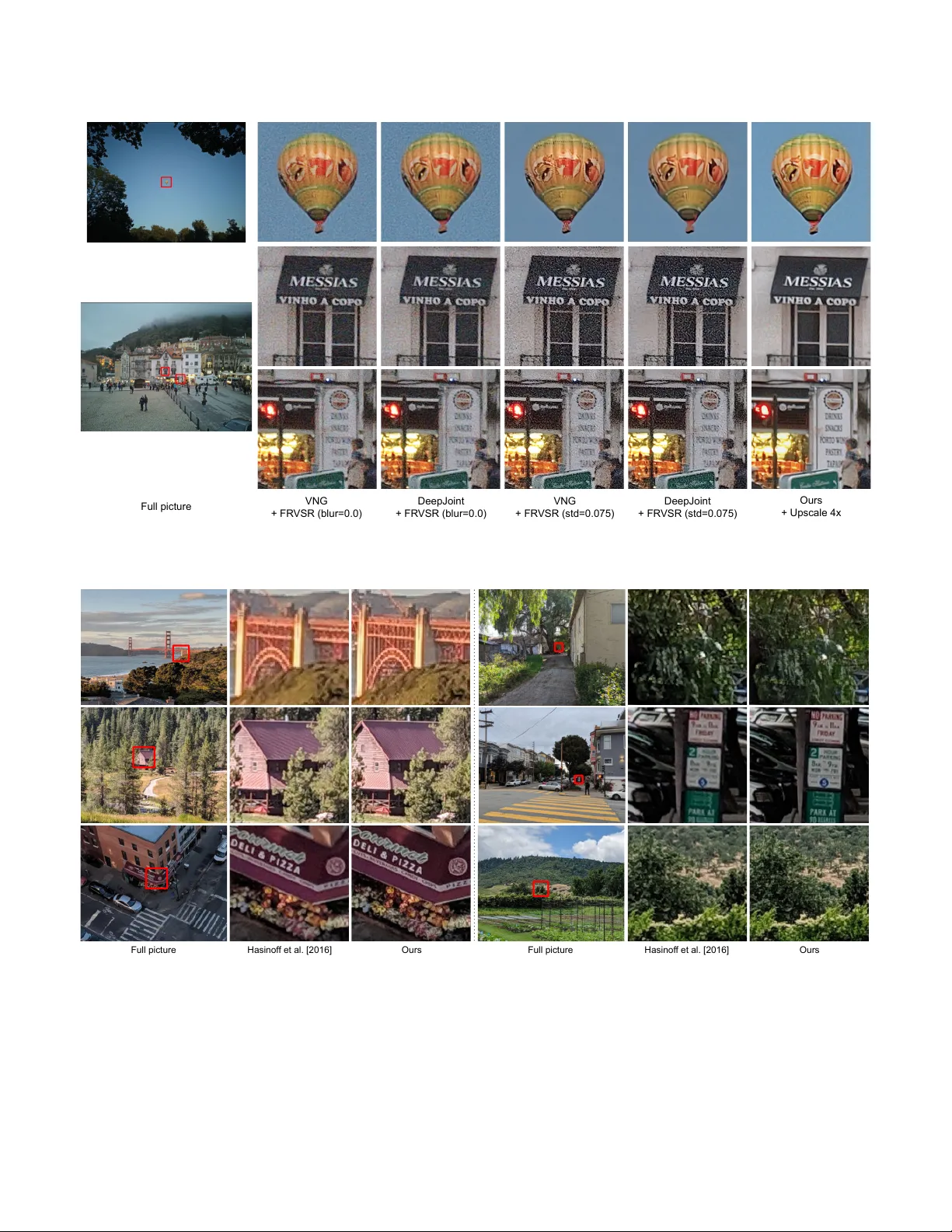
Handheld Multi-Frame Super-Resolution BARTLOMIEJ WRONSKI, IGNA CIO GARCIA -DORADO, MANFRED ERNST, D AMIEN KELL Y, MICHAEL KRAININ, CHIA -KAI LIANG, MARC LEV O Y, and PEYMAN MILANF AR, Google Research Fig. 1. W e present a multi-frame super-resolution algorithm that supplants the need for demosaicing in a camera pipeline by merging a burst of raw images. W e show a comparison to a method that merges frames containing the same-color channels together first, and is then follow ed by demosaicing ( top ). By contrast, our method ( boom ) cr eates the full RGB dir ectly from a burst of raw images. This burst was captur ed with a hand-held mobile phone and processed on device. Note in the third (r ed) inset that the demosaice d result exhibits aliasing (Moiré), while our result takes advantage of this aliasing, which changes on every frame in the burst, to produce a merged result in which the aliasing is gone but the cloth texture becomes visible. Compared to DSLR cameras, smartphone cameras have smaller sensors, which limits their spatial resolution; smaller apertures, which limits their light gathering ability; and smaller pixels, which reduces their signal-to- noise ratio . The use of color lter arrays (CF As) r equires demosaicing, which further degrades resolution. In this paper , we supplant the use of traditional demosaicing in single-frame and burst photography pipelines with a multi- frame super-resolution algorithm that cr eates a complete RGB image directly from a burst of CF A raw images. W e harness natural hand tremor , typical in handheld photography , to acquire a burst of raw frames with small osets. These frames are then aligned and merged to form a single image with red, green, and blue values at every pixel site. This approach, which includes no explicit demosaicing step, serves to b oth increase image resolution and boost signal to noise ratio. Our algorithm is robust to challenging scene conditions: local motion, occlusion, or scene changes. It runs at 100 milliseconds per 12-megapixel RA W input burst frame on mass-produced mobile phones. Specically , the algorithm is the basis of the Sup er-Res Zoom feature, as well as the default merge method in Night Sight mo de (whether zooming or not) on Google’s agship phone. Authors’ address: Bartlomiej W ronski, bwronski@google.com; Ignacio Garcia- Dorado, ignaciod@google.com; Manfred Ernst, ernstm@google.com; Damien Kelly, damienkelly@google.com; Michael Krainin, mkrainin@google.com; Chia-Kai Liang, ckliang@google.com; Marc Levo y, levoy@google.com; Peyman Milanfar , milanfar@ google.com Google Research, 1600 Amphitheatre Parkway , Mountain View, CA, 94043. Permission to make digital or hard copies of part or all of this work for p ersonal or classroom use is granted without fee provided that copies are not made or distributed for prot or commercial advantage and that copies bear this notice and the full citation on the rst page. Cop yrights for third-party components of this work must be honored. For all other uses, contact the owner /author(s). © 2019 Copyright held by the owner/author(s). 0730-0301/2019/7- ART28 https://doi.org/10.1145/3306346.3323024 CCS Concepts: • Computing methodologies → Computational pho- tography ; Image processing . Additional Key W ords and Phrases: computational photography , super- resolution, image processing, photography A CM Reference Format: Bartlomiej W ronski, Ignacio Garcia-Dorado, Manfred Ernst, Damien Kelly, Michael Krainin, Chia-Kai Liang, Mar c Levoy, and Peyman Milanfar. 2019. Handheld Multi-Frame Super-Resolution. A CM Trans. Graph. 38, 4, Article 28 ( July 2019), 24 pages. https://doi.org/10.1145/3306346.3323024 1 IN TRODUCTION Smartphone camera technology has advanced to the p oint that tak- ing pictures with a smartphone has become the most p opular form of photography [CIP A 2018; Flickr 2017]. Smartphone photography oers high portability and convenience, but many challenges still exist in the hardware and software design of a smartphone cam- era that must be overcome to enable it to compete with dedicate d cameras. Foremost among these challenges is limited spatial resolution. The r esolution produced by digital image sensors is limited not only by the physical pixel count (e.g., 12-megapixel camera), but also by the presence of color lter arrays (CF A) 1 like the Bayer CF A [Bayer 1976]. Given that human vision is more sensitive to green, a quad of pixels in the sensor usually follows the Bayer pattern RGGB; i.e., 50% green, 25% red, and 25% blue . The nal full-color image is generated from the spatially undersampled color channels through an interpolation process called demosaicing [Li et al. 2008]. 1 Also known as a color lter mosaic (CFM). ACM T rans. Graph., V ol. 38, No. 4, Article 28. Publication date: July 2019. 28:2 • W ronski et al. Demosaicing algorithms operate on the assumption that the color of an area in a given image is relatively constant. Under this as- sumption, the color channels are highly correlated, and the aim of demosaicing is to reconstruct the undersampled color informa- tion while avoiding the introduction of any visual artifacts. T ypical artifacts of demosaicing include false color artifacts such as chro- matic aliases, zippering (abrupt or unnatural changes of intensity over consecutive pixels that look like a zipper), maze, false gradient, and Moiré patterns (Figure 1 top). Often, the challenge in eective demosaicing is trading o resolution and detail recovery against introducing visual artifacts. In some cases, the underlying assump- tion of cross-channel correlation is violated, resulting in reduced resolution and loss of details. A signicant advancement in smartphone camera technology in recent years has been the application of software-based computa- tional photography techniques to over come limitations in camera hardware design. Examples include te chniques for increasing dy- namic range [Hasino et al. 2016], improving signal-to-noise ratio through denoising [Godard et al . 2018; Mildenhall et al . 2018] and wide aperture eects to synthesize shallow depth-of-eld [W adhwa et al . 2018]. Many of these recent advancements have been achieved through the introduction of burst processing 2 where on a shutter press multiple acquired images are combined to produce a photo that is of greater quality than that of a single acquired image. In this paper , we introduce an algorithm that uses signals cap- tured across multiple shifted frames to produce higher resolution images (Figure 1 bottom). Although the underlying techniques can be generalized to any shifted signals, in this work we focus on ap- plying the algorithm to the task of resolution enhancement and denoising in a smartphone image acquisition pipeline using burst processing. By using a multi-frame pipeline and combining dierent undersampled and shifted information present in dierent frames, we remov e the nee d for an explicit demosaicing step. T o work on a smartphone camera, any such algorithm must: • W ork handheld from a single shutter press – without a tripod or deliberate motion of the camera by the user . • Run at an interactive rate – the algorithm should produce the nal enhanced resolution with low latency (within at most a few seconds). • Be robust to local motion and scene changes – users might capture scenes with fast moving objects or scene changes. While the algorithm might not increase r esolution in all such scenarios, it should not produce appreciable artifacts. • Be robust to noisy input data – in low light the algorithm should not amplify noise, and should strive to reduce it. With these criteria in mind, we have developed an algorithm that processes multiple successively captur ed raw frames in an online fashion. The algorithm tackles the tasks of demosaicing and super- resolution jointly and formulates the problem as the reconstruction and interpolation of a continuous signal from a set of sparse samples. Red, green and blue pixels are treated as separate signals on dierent planes and reconstructed simultane ously . This approach enables the 2 W e use the terms multi-frame and burst processing interchangeably to refer to the process of generating a single image from multiple images captured in rapid succession. production of highly detailed images even when ther e is no cross- channel correlation – as in the case of saturated single-channel colors. The algorithm requires no spe cial capturing conditions; nat- ural hand-motion produces osets that are suciently random in the subpixel domain to apply multi-frame sup er-resolution. Addi- tionally , since our super-resolution approach creates a continuous representation of the input, it allows us to directly create an image with a desired target magnication / zoom factor without the nee d for additional resampling. The algorithm works on a mobile device and incurs a computational cost of only 100 ms per 12-megapixel processed frame. The main contributions of this work are: (1) Replacing raw image demosaicing with a multi-frame super- resolution algorithm. (2) The introduction of an adaptive kernel interpolation / merge method from sparse samples (Section 5) that takes into ac- count the local structure of the image, and adapts accordingly . (3) A motion robustness model (Section 5.2) that allo ws the algo- rithm to work with bursts containing local motion, disocclu- sions, and alignment/registration failures (Figure 12). (4) The analysis of natural hand tremor as the sour ce of subpixel coverage sucient for super-resolution (Section 4). 2 BA CKGROUND 2.1 Demosaicing Demosaicing has been studied extensively [Li et al . 2008], and the literature presents a wide range of algorithms. Most methods inter- polate the missing green pixels rst (since they have double sam- pling density) and reconstruct the red and blue pixel values using color ratio [Lukac and P lataniotis 2004] or color dierence [Hi- rakawa and Parks 2006]. Other approaches w ork in the frequency domain [Leung et al . 2011], residual space [Monno et al . 2015], use LAB homogeneity metrics [Hirakawa and Parks 2005] or non local approaches [Duran and Buades 2014]. More recent w orks use CNNs to solve the demosaicing pr oblem such as the joint demosaicing and denoising technique by Gharbi et al. [2016]. Their key insight is to create a better training set by dening metrics and techniques for mining dicult patches from community photographs. 2.2 Multi-frame Super-resolution (SR) Single-image approaches exploit strong priors or training data. They can suppress aliasing 3 well, but are often limited in how much they can reconstruct from aliasing. In contrast to single frame techniques, the goal of multi-frame super-resolution is to increase the true (optical) resolution. In the sampling theory literature, multi-frame super-resolution techniques date as far back as the ’50s [Y en 1956] and the ’70s [Pa- poulis 1977]. The work of T sai [1984] started the modern concept of sup er-resolution by showing that it was possible to improve resolution by registering and fusing multiple aliase d images. Irani and Peleg [1991], and then Elad and Feuer [1997] formulate d the 3 In this work we refer to aliasing in signal processing terms – a signal with frequency content above half of the sampling rate that manifests as a lower frequency after sampling [Nyquist 1928]. ACM T rans. Graph., V ol. 38, No. 4, Article 28. Publication date: July 2019. Handheld Multi-Frame Super-Resolution • 28:3 a) RA W Input Burst b) Local Gradients d) Alignment V ectors e) Local Statistics c) Kernels f) Motion Robustness g) Accumulation h) Merged Result Fig. 2. Overview of our method: A captured burst of raw (Bayer CF A) images (a) is the input to our algorithm. Every frame is aligned lo cally (d) to a single frame, called the base frame . W e estimate each frame ’s contribution at every pixel through kernel r egression (Section 5.1). These contributions are accumulated separately per color channel (g) . The kernel shapes (c) are adjusted based on the estimated local gradients (b) and the sample contributions are w eighted based on a robustness model (f ) (Section 5.2). This robustness model computes a per-pixel weight for ev ery frame using the alignment field (d) and local statistics (e) gathered from the neighborhood around each pixel. The final merged RGB image (h) is obtained by normalizing the accumulated results per channel. W e call the steps depicted in (b) - (g) the merge . algorithmic side of super-resolution. The ne ed for accurate sub- pixel registration, existence of aliasing, and goo d signal-to-noise levels wer e identied as the main requirements of practical super- resolution [Baker and Kanade 2002; Robinson and Milanfar 2004, 2006]. In the early 2000s, Farsiu et al. [2006] and Gotoh and Okutomi [2004] formulated super-resolution from arbitrary motion as an optimiza- tion pr oblem that w ould be infeasible for interactive rates. Ben-Ezra et al. [2005] created a jitter camera prototype to do super-resolution using controlled subpixel detector shifts. This and other works in- spired some commercial cameras (e .g., Sony A6000 , Pentax FF K1 , Olympus OM-D E-M1 or Panasonic Lumix DC-G9 ) to adopt multi- frame techniques, using controlled pixel shifting of the physical sensor . However , these approaches require the use of a tripod or a static scene. Video super-resolution approaches [Belekos et al . 2010; Liu and Sun 2011; Sajjadi et al . 2018] counter those limitations and extend the idea of multi-frame super-resolution to video sequences. 2.3 Kernel Based Super-resolution and Interpolation T akeda et al. [2006; 2007] formulated super-resolution as a kernel regression and reconstruction problem, which allows for faster pro- cessing. Around the same time, Müller et al. [2005] introduced a technique to model uid-uid interactions that can be rendered us- ing kernel methods introduced by Blinn [1982]. Y u and Turk [2013] proposed an adaptive solution to the r econstructing of surfaces of particle-based uids using anisotropic kernels. These kernels, like T akeda et al. ’s, are based on local gradient Principal Component Analysis (PCA), where the anisotropy of the kernels allows for si- multaneous preservation of sharp features and smooth rendering of at surfaces. Similar adaptive kernel based method were proposed for single image super-resolution by Hunt [2004] and for general upscaling and interpolation by Lee and Y oon [2010]. W e adopt some of these ideas and generalize them to t our use case. 2.4 Burst Photography and Raw Fusion Burst fusion methods based on raw imagery are relatively uncom- mon in the literature, as the y require knowledge of the photographic pipeline [Farsiu et al . 2006; Gotoh and Okutomi 2004; Heide et al . 2014; W u and Zhang 2006]. V andewalle et al. [2007] described an al- gorithm where information from multiple Bayer frames is separate d into luminance and chrominance components and fused together to improve the CF A demosaicing. Most relevant to our work is Hasino et al. [2016] which introduced an end-to-end burst photography pipeline fusing multiple frames for increased dynamic range and signal-to-noise ratio. Our paper is a more general fusion approach that (a) dispenses with demosaicing, (b) produces increased reso- lution, and (c) enables merging onto an arbitrary grid, allowing for high quality digital zo om at modest factors (Section 7). Most recently , Li et al. [2018] proposed an optimization based algorithm for forming an RGB image directly from fused, unregistered raw frames. 2.5 Multi-frame Rendering This work also draws on multi-frame and temporal super-resolution techniques widely used in real-time rendering (for example , in video games). Herzog et al. combined information from multiple r endered frames to increase resolution [2010]. Sousa et al. [2011] mentioned the rst commercial use of robustly combining information from two frames in real-time in a video game, while Malan [2012] expanded its use to produce a 1920 × 1080 image from four 1280 × 720 frames. ACM T rans. Graph., V ol. 38, No. 4, Article 28. Publication date: July 2019. 28:4 • W ronski et al. Subsequent work [Drobot 2014; Karis 2014; Sousa 2013] established temporal super-resolution techniques as state-of-the-art and stan- dard in real-time r endering for various eects, including dynamic resolution rendering and temporal denoising. Salvi [2016] provided a theoretical explanation of commonly used local color neighborhood clipping techniques and proposed an alternative based on statistical analysis. While most of those ideas are used in a dierent context, we generalize their insights about detecting aliasing, misalignment and occlusion in our robustness model. 2.6 Natural Hand Tr emor While holding a camera (or any obje ct), a natural, involuntary hand tremor is always present. The tremor is comprised of low amplitude and high frequency motion components that occur while holding steady limb postures [Schäfer 1886]. The movement is highly peri- odic, with a frequency in the range of 8–12 Hz, and its movement is small in magnitude but random [Marshall and W alsh 1956]. The mo- tion also consists of a mechanical-reex component that depends on the limb , and a second component that causes micro-contractions in the limb muscles [Riviere et al . 1998]. This behavior has been sho wn to not change with age [Sturman et al . 2005] but it can change due to disease [NIH 2018]. In this paper , we show that the hand tremor of a user holding a mobile camera is sucient to pr ovide subpixel coverage for super-resolution. 3 O VERVIEW OF OUR METHOD Our approach is visualized in Figure 2. First, a burst of raw (CF A Bayer) images is captured. For every captured frame, we align it locally with a single frame from the burst (called the base frame ). Next, we estimate each frame ’s local contributions through kernel regression (Section 5.1) and accumulate those contributions across the entire burst. The contributions are accumulated separately per color plane. W e adjust kernel shapes based on the estimated signal features and w eight the sample contributions based on a robustness model (Se ction 5.2). W e perform per-channel normalization to obtain the nal merged RGB image. 3.1 Frame Acquisition Since our algorithm is designed to work within a typical burst pro- cessing pip eline, it is important that the processing does not increase the overall photo capture latency . T ypically , a smartphone operates in a mode called Zero-Shutter Lag , where raw frames are b eing captured continuously to a ring buer when the user opens and operates the camera application. On a shutter pr ess, the most recent captured frames are sent to the camera processing pipeline. Our al- gorithm operates on an input burst (Figur e 2 (a)) formed from those images. Relying on previously captur ed frames creates challenges for the super-resolution algorithm – the user can b e freely moving the camera prior to the capture. The merge process must be able to deal with natural hand motion (Se ction 4) and cannot require additional movement or user actions. 3.2 Frame Registration and Alignment Prior to combining frames, we place them into a common co ordinate system by registering frames against the base frame to create a set of alignment vectors (Figure 2 (d)). Our alignment solution is a rened version of the algorithm used by Hasino et al. [2016]. The core alignment algorithm is coarse-to-ne, pyramid-based blo ck matching that creates a pyramid representation of every input frame and performs a limited window search to nd the most similar tile. Through the alignment process we obtain p er patch/tile (with tile sizes of 𝑇 𝑠 ) alignment vectors relative to the base frame. Unlike Hasino et al. [2016], we require subpixel accurate align- ment to achieve super-resolution. T o address this issue we could use a dierent, dedicated registration algorithm designed for accurate subpixel estimation (e.g., Fleet and Jepson [1990]), or rene the block matching results. W e opted for the latter due to its simplicity and computational ecency . W e have explored estimating the subpixel osets by tting a quadratic curve to the blo ck matching align- ment error and nding its minimum [K anade and Okutomi 1991]; howev er , we found that super-resolution requires a mor e accurate method. Therefore, we rene the block matching alignment vectors by three iterations of Lucas-K anade [1981] optical ow image warp- ing. This approach reached the necessary accuracy while keeping the computational cost low . 3.3 Merge Process After frames are aligned, the remainder of the merge pr ocess (Fig- ure 2 (b-g)) is responsible for fusing the raw frames into a full RGB image. These steps constitute the core of our algorithm and will be described in greater detail in Section 5. The merge algorithm works in an online fashion, se quentially computing the contributions of each processed frame to every out- put pixel by accumulating colors from a 3 × 3 neighborhoo d. Those contributions are weighted by kernel weights (Section 5.1, Figure 2 (c)), modulated by the robustness mask (Section 5.2, Figure 2 (f )), and summed together separately for the red, green and blue color planes. At the end of the process, we divide the accumulated color contributions by the accumulated weights, obtaining three color planes. The result of the merge process is a full RGB image, which can be dened at any desired resolution. This can be processe d further by the typical camera pipeline (spatial denoising, color correction, tone-mapping, sharpening) or alternatively saved for further oine processing in a non-CF A raw format like Linear DNG [Adobe 2012]. Before we explain the algorithm details, we analyze the key char- acteristics that enable the hand-held super-resolution. 4 HAND-HELD SUPER-RESOLU TION Multi-frame super-resolution requires two conditions to be ful- lled [T sai and Huang 1984]: (1) Input frames need to b e aliased, i.e., contain high frequen- cies that manifest themselves as false low frequencies after sampling. (2) The input must contain multiple aliased images, sampled at dierent subpixel osets. This will manifest as dierent phases of false low frequencies in the input frames. Having multiple lower resolution shifted and aliased images allows us to both remove the eects of aliasing in low frequencies as well as reconstruct the high frequencies. In a (mobile) camera pipeline, ACM T rans. Graph., V ol. 38, No. 4, Article 28. Publication date: July 2019. Handheld Multi-Frame Super-Resolution • 28:5 -1.5 -1 -0.5 0 0.5 1 1.5 Horizontal Angular Displacement (radians 10 -3 ) -1.5 -1 -0.5 0 0.5 1 1.5 Vertical Angular Displacement (radians 10 -3 ) 0 0.05 0.1 0.15 0.2 0.25 0.3 0.3 5 Angular Velocity (radians/sec) 0 0.05 0.1 0.15 0.2 Bin Count / Total Count a) b) Fig. 3. (a) Horizontal and vertical angular displacement (i.e., not including translational displacement) arising from handheld motion evaluated over a test set of 86 captured bursts. The red circle corr esponds to one standard deviation (which maps to a pixel displacement magnitude of 0.89 pixels ) showing that the distribution is roughly symmetrical. (b) Histogram of angular velocity magnitude measured over the test set showing that during captures the rotational velocity remains r elatively low . ( 1 ) means an image sensor having distances between pixels larger than the spot size of the lens. Our algorithm assumes that the input raw frames are aliased (see discussion in Section 7). Most existing multi-frame super-resolution approaches impose restrictions on the types of motion noted in ( 2 ) . This includes com- mercially available products like DSLR cameras using sensor shifts of a camera placed on a trip od. Those requirements are impractical for casual photography and violate our algorithm goals; therefor e we make use of natural hand motion. Some publications like Li et al. [2018] use unregister ed, randomly oset images for the pur- pose of super-resolution or multi-frame demosaicing, ho wever to our knowledge no prior work analyzes if the subpixel coverage produced by hand tremor is sucient to obtain consistent results. W e show that using hand tremor alone is enough to move the de vice adequately during the burst acquisition. T o analyze the actual b ehavior when capturing bursts of pho- tographs while holding a mobile device, we hav e examined the hand movement in a set of 86 bursts. The analyze d bursts were captured by 10 dierent users during casual photography and not for the purpose of this experiment. Mobile devices pro vide precise informa- tion about rotational movement measured by a gyroscope, which we use in our analysis. As we lack measurements about translation of the device, w e ignore translations in this analysis, although we recognize that the y also occur . In Section 5.2, we sho w how our algo- rithm is robust to parallax, and occlusions or disocclusions, caused by translational camera displacement. First, we used the phone gyroscope rotational velocity measure- ments and integrate d them to nd the relativ e rotation of the phone compared to the burst capture start. W e plotted them along with a histogram of angular velocities in Figure 3. Our analysis con- rms that the hand movement introduces uniformly random (no directions are preferred) angular displacements and relatively slow rotation of the capture device during the burst acquisition. The fol- lowing section analyzes movement in the subpixel space and how it facilitates random sampling. 4.1 Handheld Motion in subpixel Space Although handshake averaged over the course of a long time interval is random and isotropic, handshake over the course of a short burst might be nearly a straight line or gentle curve in X- Y [Hee Park and Levoy 2014]. Will this provide a uniform enough distribution of subpixel samples? It does, but for non-obvious reasons. Consider each pixel as a point sample, and assume a pessimistic, least random scenario – that the hand motion is regular and lin- ear . After alignment to the base frame, the p oint samples from all frames combined will be approximately uniformly distributed in the subpixel space (Figure 4). This follows from the equidistribution theorem [W eyl 1910], which states that the sequence { 𝑎, 2 𝑎, 3 𝑎, . . . mod 1 } is uniformly distributed (if 𝑎 is an irrational number). Note that while the equidistribution the orem assumes innite sequences, the closely related concept of rank-1 lattices is use d in practice to generate nite point sets with low discrepancy for image synthe- sis [Dammertz and Keller 2008] in computer graphics. Obviously , not all the assumptions above hold in practice. There- fore, we veried empirically that the resulting sample locations are indeed distributed as expected. W e measured the subpixel osets by registration (Section 3.2) for 16 × 16 tiles aggregated across 20 handheld burst sequences. The biggest deviation from a uniform distribution is caused by a phenomenon known as pixel locking and is visible in the histogram as bias towards whole pixel values. As can be seen in Figure 5, pixel lo cking causes non-uniformity in the distribution of subpixel displacements. Pixel locking is an artifact of any subpixel registration process [Robinson and Milanfar 2004; Shimiziu and Okutomi 2005] that depends on the image content (high spatial frequencies and more aliasing cause a str onger bias). Despite this eect, the subpixel coverage of displacements remains suciently large in the range ( 0 , 1 ) to motivate the application of super-resolution. 5 PROPOSED MULTI-FRAME SUPER-RESOLU TION APPRO ACH Super-resolution techniques reconstruct a high resolution signal from multiple lower resolution representations. Given the stochastic nature of pixel shifts resulting from natural hand motion, a good reconstruction technique to use in our case is kernel regression (Section 5.1) that reconstructs a continuous signal. Such continu- ous representation can be resampled at any r esolution equal to or higher than the original input frame resolution (see Section 7 for discussion of the eective resolution). W e use anisotropic Gaussian Radial Basis Function (RBF) kernels (Section 5.1.1) that allow for locally adaptive detail enhancement or spatio-temporal denoising. Finally , we present a robustness model (Se ction 5.2) that allows our algorithm to work in scenes with complex motion and to degrade gracefully to single frame upsampling in cases where alignment fails. ACM T rans. Graph., V ol. 38, No. 4, Article 28. Publication date: July 2019. 28:6 • W ronski et al. 1 st frame (base frame) 2 nd frame 3 rd frame 4 th frame All frames aligned to base frame Fig. 4. Subpixel displacements from handheld motion: Illustration of a burst of four frames with linear hand motion. Each frame is oset from the previous frame by half a pixel along the x-axis and a quarter pixel along the y-axis due to the hand motion. Aer alignment to the base frame, the pixel centers (black dots) uniformly cov er the resampling grid ( grey lines) at an incr eased density . In practice, the distribution is more random than in this simplifie d example. 0.05 0.15 0.25 0.35 0.45 0.55 0.65 0.75 0.85 0.95 Sub-pixel Displacement 0 0.05 0.1 0.15 Bin Count / Total Count x displacement y displacement Fig. 5. Distribution of estimate d subpixel displacements: Histogram of x and y subpixel displacements as computed by the alignment algorithm (Section 3.2). While the alignment process is biase d towards whole-pixel values, we observe suicient coverage of subpixel values to motivate sup er- resolution. Note that displacements in x and y are not correlated. 5.1 Kernel Reconstruction The core of our algorithm is built on the idea of treating pixels of multiple raw Bayer frames as irregularly oset, aliased and noisy measurements of three dierent underlying continuous signals, one for each color channel of the Bayer mosaic. Though the color channels are often correlated, in the case of saturate d colors (for example red, green or blue only) they are not. Given sucient spatial coverage, separate per-channel reconstruction allows us to r ecover the original high resolution signal even in those cases. T o produce the nal output image we processes all frames se quen- tially – for ev er y output image pixel, w e evaluate local contributions to the red, green and blue color channels from dierent input frames. Every input raw image pixel has a dierent color channel, and it con- tributes only to a spe cic output color channel. Lo cal contributions are weighted; therefore , we accumulate weighted contributions and weights. At the end of the pipeline, those contributions are normal- ized. For each color channel, this can be formulated as: 𝐶 ( 𝑥 , 𝑦 ) = Í 𝑛 Í 𝑖 𝑐 𝑛,𝑖 · 𝑤 𝑛,𝑖 · ˆ 𝑅 𝑛 Í 𝑛 Í 𝑖 𝑤 𝑛,𝑖 · ˆ 𝑅 𝑛 , (1) E dge F lat Det ailed A rea Fig. 6. Sparse data reconstruction with anisotropic kernels: Exagger- ated example of very sharp (i.e., narrow , 𝑘 𝑑 𝑒 𝑡 𝑎𝑖𝑙 = 0 . 05 𝑝 𝑥 ) kernels on a real captured burst. For demonstration purposes, we r epresent samples corre- sponding to whole RGB input pictures instead of separate color channels. Kernel adaptation allo ws us to apply dierently shaped kernels on edges (orange), flat ( blue) or detailed areas (green). The orange kernel is aligned with the edge, the blue one covers a large area as the region is f lat, and the green one is small to enhance the resolution in the presence of details. where ( 𝑥 , 𝑦 ) are the pixel coordinates, the sum Í 𝑛 is over all con- tributing frames, Í 𝑖 is a sum over samples within a local neighb or- hood (in our case 3 × 3), 𝑐 𝑛,𝑖 denotes the value of the Bayer pixel at given frame 𝑛 and sample 𝑖 , 𝑤 𝑛,𝑖 is the local sample weight and ˆ 𝑅 𝑛 is the local robustness (Section 5.2). In the case of the base frame , ˆ 𝑅 is equal to 1 as it does not get aligned, and we have full condence in its local sample values. T o compute the local pixel weights, we use local radial basis function kernels, similarly to the non-parametric kernel regression framework of T akeda et al. [2006; 2007]. Unlike T ake da et al., we don’t determine kernel basis function parameters at sparse sample positions. Instead, we evaluate them at the nal resampling grid positions. Furthermore, we always look at the nine closest sam- ples in a 3 × 3 neighb orhood and use the same kernel function for all those samples. This allows for ecient parallel evaluation on a GP U. Using this "gather" approach every output pixel is indep en- dently processed only once per frame. This is similar to work of ACM T rans. Graph., V ol. 38, No. 4, Article 28. Publication date: July 2019. Handheld Multi-Frame Super-Resolution • 28:7 Fig. 7. Anisotropic Kernels: Le: When isotropic kernels ( 𝑘 𝑠 𝑡 𝑟 𝑒 𝑡 𝑐ℎ = 1 , 𝑘 𝑠ℎ𝑟 𝑖 𝑛𝑘 = 1 , see supplemental material) are used, small misalignments cause heavy zipper artifacts along edges. Right: Anisotropic kernels ( 𝑘 𝑠 𝑡 𝑟 𝑒 𝑡 𝑐ℎ = 4 , 𝑘 𝑠ℎ𝑟 𝑖 𝑛𝑘 = 2 ) fix the artifacts. Y u and T urk [2013], developed for uid rendering. T wo steps de- scribed in the following sections are: estimation of the kernel shape (Section 5.1.1) and robustness based sample contribution weighting (Section 5.2). 5.1.1 Lo cal A nisotropic Merge Kernels. Given our pr oblem formula- tion, kernel weights and kernel functions dene the image quality of the nal merge d image: kernels with wide spatial support pro- duce noise-free and artifact-free, but blurr y images, while kernels with v er y narro w support can produce sharp and detailed images. A natural choice for kernels used for signal reconstruction are Radial Basis Function kernels - in our case anisotropic Gaussian kernels. W e can adjust the kernel shape to dierent local pr operties of the input frames: amounts of detail and the presence of edges (Figure 6). This is similar to kernel selection techniques used in other sparse data reconstruction applications [T akeda et al . 2006, 2007; Y u and T urk 2013]. Specically , we use a 2D unnormalized anisotropic Gaussian RBF for 𝑤 𝑛,𝑖 : 𝑤 𝑛,𝑖 = exp − 1 2 𝑑 𝑇 𝑖 Ω − 1 𝑑 𝑖 , (2) where Ω is the kernel covariance matrix and 𝑑 𝑖 is the oset vector of sample 𝑖 to the output pixel ( 𝑑 𝑖 = [ 𝑥 𝑖 − 𝑥 0 , 𝑦 𝑖 − 𝑦 0 ] 𝑇 ). One of the main motivations for using anisotropic kernels is that they increase the algorithm’s tolerance for small misalignments and uneven coverage around edges. Edges are ambiguous in the alignment procedure (due to the aperture problem) and result in alignment errors [Robinson and Milanfar 2004] more frequently compared to non-edge regions of the image. Subpixel misalignment as w ell as a lack of sucient sample coverage can manifest as zipper artifacts (Figure 7). By stretching the kernels along the edges, we can enforce the assignment of smaller weights to pixels not b elonging to edges in the image. 5.1.2 Kernel Co variance Computation. W e compute the kernel co- variance matrix by analyzing every frame’s local gradient structure tensor . T o improve runtime performance and resistance to image noise, we analyze gradients of half-resolution images forme d by decimating the original raw frames by a factor of two. T o decimate a Bayer image containing dierent color channels, we create a single P resence of an edge P resence of a sharp f eat ure 1. 0 0. 8 0. 6 0. 4 0. 2 0. 0 0. 1 0. 5 0. 9 0. 01 0. 015 0. 03 Fig. 8. Merge kernels: Plots of relative weights in dierent 3 × 3 sampling kernels as a function of local tensor features. pixel from a 2 × 2 Bayer quad by combining four dierent color channels together . This way , we can operate on single channel lumi- nance images and perform the computation at a quarter of the full resolution cost and with impr oved signal-to-noise ratio. T o estimate local information about strength and direction of gradients, we use gradient structure tensor analysis [Bigün et al . 1991; Harris and Stephens 1988]: b Ω = 𝐼 2 𝑥 𝐼 𝑥 𝐼 𝑦 𝐼 𝑥 𝐼 𝑦 𝐼 2 𝑦 , (3) where 𝐼 𝑥 and 𝐼 𝑦 are the lo cal image gradients in horizontal and vertical directions, respectively . The image gradients are computed by nite forward dierencing the luminance in a small, 3 × 3 color window (giving us four dierent horizontal and vertical gradient values). Eigenanalysis of the local structure tensor b Ω gives two orthogonal direction vectors e 1 , e 2 and two associated eigenvalues 𝜆 1 , 𝜆 2 . From this, we can construct the kernel covariance as: Ω = e 1 e 2 𝑘 1 0 0 𝑘 2 e 𝑇 1 e 𝑇 2 , (4) where 𝑘 1 and 𝑘 2 control the desired kernel variance in either edge or orthogonal direction. W e control those values to achieve adaptiv e super-resolution and denoising. W e use the magnitude of the struc- ture tensor’s dominant eigenvalue 𝜆 1 to drive the spatial supp ort of the kernel and the trade-o between the super-resolution and denoising, where 𝜆 1 − 𝜆 2 𝜆 1 + 𝜆 2 is used to drive the desired anisotropy of the kernels (Figure 8). The specic process we use to compute the nal kernel covariance can be found in the supplemental material along with the tuning values. Since Ω is computed at half of the Bayer image resolution, we upsample the kernel covariance values through bilinear sampling before computing the kernel weights. 5.2 Motion Robustness Reliable alignment of an arbitrary sequence of images is extremely challenging – because of both theoretical [Robinson and Milanfar 2004] and practical (available computational p ower ) limitations. Even assuming the existence of a perfect registration algorithm, changes in scene and occlusion can result in some areas of the photographed scene b eing unrepresented in many frames of the ACM T rans. Graph., V ol. 38, No. 4, Article 28. Publication date: July 2019. 28:8 • W ronski et al. Fig. 9. Motion robustness: Le: Photograph of a moving bus without any robustness model. Alignment errors and occlusions correspond to severe tiling and ghosting artifacts. Middle: an accumulated robustness mask produced by our model. White regions correspond to all frames geing merged and contributing to super-resolution, while dark regions have a smaller number of merged frames because of motion or incorrect alignment. Right: result of merging frames with the robustness model. sequence. Without taking this into account, the multi-frame fusion process as described so far would produce strong artifacts. T o fuse any sequence of frames robustly , we assign condence to the lo cal neighborhood of every pixel that we consider merging. W e call an image map with those condences a robustness mask where a value of one corresponds to fully merged regions and value of zero to rejected areas (Figure 9). 5.2.1 Statistical Robustness Model. The core idea behind our ro- bustness logic is to address the following question: how can we dis- tinguish between aliasing, which is necessar y for super-resolution, and frame misalignment which hampers it? W e observe that areas prone to aliasing have large spatial variance even within a single frame. This idea has previously been successfully used in temporal anti-aliasing techniques for real-time graphics [Salvi 2016]. Though our application in fusing information from multiple frames is dier- ent, we use a similar local variance computation to nd the highly aliased areas. W e compute the lo cal standard deviation in the images 𝜎 and a color dierence b etween the base frame and the aligne d input frame 𝑑 . Regions with dierences smaller than the local stan- dard deviation are deemed to be non-aliased and are merged, which contributes to temp oral denoising. Dier ences close to a pre-dened fraction of spatial standard deviation 4 are deemed to be aliased and are also merged, which contributes to super-resolution. Dier- ences larger than this fraction most likely signify misalignments or non-aligne d motion, and are discarded. Through this analysis, we interpret the dierence in terms of standard deviations (Fig- ure 10) as the probability of frames b eing safe to merge using a soft comparison function: 𝑅 = 𝑠 · exp − 𝑑 2 𝜎 2 − 𝑡 , (5) where 𝑠 and 𝑡 are tune d scale and threshold parameters used to guarantee that small dierences get a weight of one, while large dierence get fully rejected. The following subse ctions will describ e how we compute 𝑑 and 𝜎 as well as how we adjust the 𝑠 tuning based on the presence of local motion. 4 that depends on the presence of the motion in the scene, see Section 5.2.3. 0 0.2 0.4 0.6 0.8 1 0 0.1 0.2 0.3 0.4 0.5 0.6 0.7 0.8 0.9 1 Robustness Misalignment Aliasing Denoising 0 0.1 0.2 0.3 0.4 0.5 0.6 0.7 0.8 0.9 1 Fig. 10. Statistical robustness model: The relationship b etween color dierence 𝑑 and local standard deviation 𝜎 dictates how we merge a given frame with respect to the base frame. a) b) d) c) Fig. 11. Noise model: T op row: well aligned low-light photo merged with- out the noise model. Boom row: The same photo merged with the noise model included. Le: Accumulated robustness mask. Right: The merged image. Including the noise mo del in the statistical comparisons helps to avoid false low confidence in the case of relatively flat, noisy regions. 5.2.2 Noise-corrected Local Statistics and Color Dier ences. First, we create a half-resolution RGB image that we call the guide image . This guide image is formed by creating a single RGB pixel corre- sponding to each Bayer quad by taking red and blue values directly and averaging the green channels together . In this section, we will ACM T rans. Graph., V ol. 38, No. 4, Article 28. Publication date: July 2019. Handheld Multi-Frame Super-Resolution • 28:9 Fig. 12. Le: Merged photograph of a moving person without any robust- ness. Misalignment causes fusion artifacts. Middle: Merged image with statistical robustness only, some artifacts are still present (we advise the reader to zoom in). Right: Final merged image with both statistical robust- ness and motion prior . Inclusion of b oth motion robustness terms helps to avoid fusion artifacts. use the following notation: subscript 𝑚𝑠 signies variables mea- sured and computed locally from the guide image, 𝑚𝑑 denotes ones computed according to the noise estimation for given brightness level, and variables without those subscripts are noise-corrected measurements. For every pixel of the guide image, we compute the color mean and spatial standard deviation 𝜎 𝑚𝑠 in a 3 × 3 neigh- borhood. The local mean is used to compute local color dierence 𝑑 𝑚𝑠 between the base frame and the aligned input frame. Since the estimates for 𝜎 𝑚𝑠 and 𝑑 𝑚𝑠 are produced from a small number of samples, we need to correct them for the expected amount of noise in the image. Raw images taken with dierent e xposure times and ISOs have dierent levels of noise. The noise present in raw images is a het- eroscedastic Gaussian noise [Foi et al . 2008], with the noise variance being a linear function of the input signal brightness. Parameters of this linear function (slope and intercept) depend on the sensor and exposure parameters, which we call the noise mo del . In low light, noise causes even correctly aligned images to have a much larger 𝑑 𝑚𝑠 dierences compared to the good lighting scenario. W e estimate the 𝜎 𝑚𝑠 and 𝑑 𝑚𝑠 from just nine samples for the red and blue color pixels ( 3 × 3 neighb orhood) and are in eect unreliable due to noise. T o correct those noisy measurements, we incorp orate the noise model in two ways: we compute the spatial color standard devia- tion 𝜎 𝑚𝑑 and mean dierences between two frames 𝑑 𝑚𝑑 that are expected on patches of constant brightness. W e obtain 𝜎 𝑚𝑑 and 𝑑 𝑚𝑑 through a series of Monte Carlo simulations for dierent brightness levels to take into account non-linearities like sensor clipping values around the white point. Modelled variables are used to clamp 𝜎 𝑚𝑠 from below by 𝜎 𝑚𝑑 and to apply a Wiener shrinkage [Kuan et al . 1985] on 𝜎 𝑚𝑠 to compute nal values of 𝜎 and 𝑑 : 𝜎 = max ( 𝜎 𝑚𝑠 , 𝜎 𝑚𝑑 ) . 𝑑 = 𝑑 𝑚𝑠 𝑑 2 𝑚𝑠 𝑑 2 𝑚𝑠 + 𝑑 2 𝑚𝑑 , (6) Inclusion of the noise model allows us to correctly merge multiple noisy frames in low-light scenario (Figure 11). 5.2.3 Additional Robustness Refinement. T o impr ove the robustness further , we use additional information that comes from analyzing local values of the alignment vectors. W e observe that in the case of just camera motion and correct alignment, the alignment eld is generally smooth. Therefore r egions with no alignment variation can b e attribute d to areas with no local motion. Combining this motion prior into the robustness calculation can remove many more artifacts, as shown in Figure 12. In the case of misalignments due to the aperture problem or presence of local motion in the scene, the local alignment shows large local variation even in the presence of strong image featur es. W e use this obser vation as an additional constraint in our robustness model. In the case of large local motion variation – computed as the length of local span of the displacement vectors magnitude – we mark such region as likely having incorrect motion estimates: 𝑀 𝑥 = max 𝑗 ∈ 𝑁 3 𝑣 𝑥 ( 𝑗 ) − min 𝑗 ∈ 𝑁 3 𝑣 𝑥 ( 𝑗 ) , 𝑀 𝑦 = max 𝑗 ∈ 𝑁 3 𝑣 𝑦 ( 𝑗 ) − min 𝑗 ∈ 𝑁 3 𝑣 𝑦 ( 𝑗 ) , 𝑀 = 𝑀 2 𝑥 + 𝑀 2 𝑦 , (7) where 𝑣 𝑥 and 𝑣 𝑦 are horizontal and vertical displacements of the tile, 𝑀 𝑥 and 𝑀 𝑦 are local motion extents in horizontal and vertical direction in a 3 × 3 neighb orhood 𝑁 3 , and 𝑀 is the nal lo cal motion strength estimation. If 𝑀 exceeds a threshold value 𝑀 𝑡 ℎ (see the supplemental material for details on the empirical tuning of 𝑀 𝑡 ℎ ), we consider such pixel to be either containing signicant lo cal displacement or be misaligne d and we use this information to scale up the robustness strength 𝑠 (Equation (5)): 𝑠 = 𝑠 1 𝑖 𝑓 𝑀 > 𝑀 𝑡 ℎ 𝑠 2 𝑜 𝑡 ℎ𝑒𝑟 𝑤 𝑖 𝑠 𝑒 (8) As a nal step in our robustness computations, we perform ad- ditional renement through morphological operations - we take a minimum condence value in a 5 × 5 window: ˆ 𝑅 = min 𝑗 ∈ 𝑁 5 𝑅 ( 𝑗 ) . (9) This way we improv e the robustness estimation in the case of mis- alignment in regions with high signal variance (like an edge on top of another one). 6 RESULTS T o evaluate the quality of our algorithm, we provide the following analysis: (1) Numerical and visual comparison against state of the art de- mosaicing algorithms using reference non-mosaic synthetic data. (2) Analysis of the ecacy of our motion robustness after intro- duction of articial corruption to the burst data. (3) Visual comparison against state of the art demosaicing al- gorithms applied to real bursts captured by a mobile phone camera. W e analyze demosaicing when applied to b oth a sin- gle frame and the results of the merge method described by Hasino et al. [2016]. (4) End-to-end quality comparison inside a camera pipeline. W e additionally investigate factors of relevance to our algorithm such as number of frames, target resolution, and computational eciency . ACM T rans. Graph., V ol. 38, No. 4, Article 28. Publication date: July 2019. 28:10 • W ronski et al. G round T rut h G round T rut h (crop) A DMM V NG DeepJoint O urs a) b) c) F lexI S P Fig. 13. Visual comparison of synthetic results. Comparison of dierent single-image demosaicing techniques with that of our algorithm. Our algorithm uses information present between multiple frames to avoid typical demosaicing artifacts and is able to reconstruct most details in the case of highly saturated color areas. 6.1 Synthetic Data Comparisons As we propose our algorithm as a replacement for the demosaic- ing step in classic camera pipelines, we compare against selected demosaicing algorithms: • V ariable Numb er of Gradients (VNG) [Chang et al . 1999] is used in the popular software open source processing to ol dcraw . • FlexISP reconstructs images using a global optimization based on a single objective function [2014]. • DeepJoint Demosaicing and Denoising is a state-of-the-art neural network based approach by Gharbi et al. [2016]. • ADMM is an optimization base d te chnique by T an et al. [2017]. T o provide numerical full reference measurements (PSNR and SSIM), we need reference data. W e create synthetic image bursts using two well-know datasets: Kodak (25 images) and McMaster (18 images) [Zhang et al . 2011]. From each image, we created a synthetic burst, i.e., we generated a set of 15 random osets ( bivariate Gaussian distribution with a standard deviation of two pixels). W e resampled the image using nearest neighbor interpolation and created a Bayer mosaic (by discarding two of three color channels) to simulate the aliasing. W e measur ed the performance of our full algorithm against the direct single frame demosaicing techniques by comparing each algorithm’s output to the original, non-resampled and non-Bay er image. T able 1 presents the average PSNR and SSIM of all evaluated techniques on both datasets ( box plots can be found in the sup- plemental material). Our algorithm is able to use the information present across multiple frames and achieves the highest PSNR ( over 3 dB better than the next best one, DeepJoint , on b oth datasets) and SSIM numbers ( 0 . 996 / 0 . 993 vs 0 . 991 / 0 . 986 ). W e additionally evaluate the results perceptually – the demosaicing algorithms are able to correctly reproduce most of the original information with an ex- ception of a few problematic areas. In Figure 13 we present some examples of demosaicing artifacts that our method avoids: color bleed (a), loss of details (b-c) and zipper artifacts ( d). In table Table 1 we also show the timings and computational performance of the used reference implementations. As our algorithm was designe d to run on a mobile device , it was highly optimized and uses a fast GP U processor , we achieve much better performance – even when merging 15 frames. T able 1. ality analysis of our algorithm on synthetic data. A verage PSNR and SSIM of selected demosaicing algorithms and our technique. Our algorithm has more information available across multiple frames and achieves the best quality results. Kodak K odak McM McM MPix/s PSNR SSIM PSNR SSIM (higher is better) ADMM 31.79 0.935 32.66 0.957 0.0005 (CP U) VNG 34.71 0.978 32.74 0.961 3.22 (CP U) FlexISP 35.08 0.967 35.15 0.975 3.07 (GP U) DeepJoint 39.67 0.991 37.58 0.986 0.33 (GPU) Ours 42.86 0.996 41.26 0.993 1756.9 (GP U) 6.2 Motion robustness eicacy T o evaluate the ecacy of motion robustness, we use the synthetic bursts generated in (Se ction 6.1) and additionally introduce two types of distortions. The rst distortion is to replace random align- ment vectors with incorrect values belonging to a dierent area of the image. This is similar to the b ehavior of real registration ACM T rans. Graph., V ol. 38, No. 4, Article 28. Publication date: July 2019. Handheld Multi-Frame Super-Resolution • 28:11 F ull pict ure O ne F rame + DeepJoint O ne F rame + V NG Hasinof f et al. [ 2016] + DeepJoint O urs Hasinof f et al. [ 2016] + V NG Fig. 14. Comparison with demosaicing techniques: Our method compared with dcraw’s V ariable Number of Gradients [Chang et al . 1999] and Deep- Joint [Gharbi et al . 2016]. Both demosaicing techniques are applie d to either one frame from a burst or result of burst merging as described in Hasino et al. [2016]. Readers are encouraged to zoom in aggressively (300% or more). algorithms in case of signicant movement and occlusion. W e cor- rupt this way with an increasing percentage of local alignment tiles 𝑝 = [ 10% , . ., 50% ] . The second type of distortion is to introduce random noise to the alignment vectors, thereby shifting each image tile by a small, random amount. This type of distortion is often cause d by the noise or aliasing in the real images, or alignment ambiguity due to the aperture problem. W e add such noise independently to each tile and use normally distributed noise with standard deviation 𝜎 = [ 0 . 05 , . ., 0 . 25 ] displacement pixels. Examples of both evaluations can be seen in (Figur e 17). Under very strong distortion, the algorithm fuses far fewer frames and behaves similarly to single-frame demosaicing algorithms. While it shows similar artifacts to the other demosaicing te chniques (color fringing, loss of detail), no multi-frame fusion artifact is present. In the supplemental material, we include the PSNR analysis of the error with increasing amount of corruption, and more examples of how our motion robustness works on many dierent real bursts containing complex local motion or scene changes. 6.3 Comparison on Real Captured Bursts W e perform comparisons on real raw bursts captured with a Google Pixel 3 phone camera. W e compar e against both single-frame demo- saicing and the spatio-temporal Wiener-lter described by Hasino et al. [2016], which also performs a burst merge. As the output of all techniques is in linear space and is blurred by the lens, we sharpen it with an unsharp mask lter (with a standard de viation of three pixels) and apply global tonemapping – an S-shaped curve with gamma correction. W e present some e xamples of this comparison in Figure 14. It shows that our algorithm produces the most detaile d images with the least amount of noise. Our results do not display artifacts like zippers in case of VNG or structured pattern noise in case of DeepJoint . W e show more examples in the supplemental material. W e also conducte d a user study to evaluate the quality of our method. For the study , we randomly generated four 250 × 250 pixel crops from each of the images presented in Figure 14. T o avoid crops with no image content, we discarded crops where the standard deviation of pixel intensity was measured to b e less than 0 . 1 . In the study , we examined all paired examples between our method ACM T rans. Graph., V ol. 38, No. 4, Article 28. Publication date: July 2019. 28:12 • W ronski et al. F ull pict ure V NG + F R V S R (blur= 0. 0) DeepJoint + F R V S R (blur= 0. 0) V NG + F R V S R (st d= 0. 075) O urs + Upscale 4x DeepJoint + F R V S R (st d= 0. 075) Fig. 15. Comparison with video super-resolution. Our method compared with FRVSR [Sajjadi et al . 2018] applied to bursts of images demosaiced with VNG [Chang et al. 1999] or DeepJoint [Gharbi et al. 2016]. Readers are encouraged to zoom aggressively (300% or more). F ull pict ure Hasinof f et al. [ 2016] O urs F ull pict ure Hasinof f et al. [ 2016] O urs Fig. 16. End-to-end comparison as a replacement for the merge and demosaicing steps used in a camera pipeline. Six bursts captured with a smartphone processed by a full camera pipeline describ ed by Hasino et al. [2016]. Image crops on the le show results of merging using a temporal Wiener filter together with demosaicing, while image crops on the right show r esults of our algorithm. Our results show higher image resolution with more visible details and no aliasing eects. ACM T rans. Graph., V ol. 38, No. 4, Article 28. Publication date: July 2019. Handheld Multi-Frame Super-Resolution • 28:13 Ref erence 20% Corrupt ed t iles 40% Corrupt ed t iles 40% corrupt ed t iles Robust ness of f Ref erence A lignment noise 0. 05 pixels A lignment noise 0. 3 pixels A lignment noise 0. 3 pixels Robust ness of f Fig. 17. Image quality degradation under misalignment. T op row: Visual quality degradation caused by randomly corrupte d and misaligned tiles. Boom row: Visual quality degradation caused by noise added to the alignment vectors. From le to right we show the outputs corresponding to progressively more corrupted input data. The far-right example shows how the algorithm would behave without the motion robustness component. W e obser ve that with increasing distortion rate, the algorithm tends to reject most frames, and results resemble a simple demosaicing algorithm with similar limitations and artifacts, but does not show fusion artifacts. T able 2. User study: W e used A mazon Mechanical T urk and asked 115 pe ople - ‘Which camera quality do y ou prefer?’ . Shown, is a confusion matrix with the participants’ nominated preference for each algorithm with respect to the other algorithms examined. Each entry is the fraction of cases where the row method was preferred relative to the column method. Our algorithm (highlighted in bold) was found to b e preferred in more that 79% of cases than that of the next best competing algorithm (Hasino et al. + DeepJoint). One Frame One Frame Hasino et al. Hasino et al. DeepJoint VNG + DeepJoint VNG Ours One Frame + DeepJoint - 0.495 0.198 0.198 0.059 One Frame + VNG 0.505 - 0.099 0.168 0.059 Hasino et al. + DeepJoint 0.802 0.901 - 0.624 0.208 Hasino et al. + VNG 0.802 0.832 0.376 - 0.099 Ours 0.941 0.941 0.792 0.901 - and the other compared methods. Using Amazon Mechanical Turk we titled each pair of crops, Camera A and Camera B , and aske d 115 people to choose their prefered camera quality by asking the question - ‘Which camera quality do you prefer?’ . The crops were displayed at 50% screen width and partipicants were limited to thr ee minutes to review each example pair (the average time spent was 45 seconds). T able 2 shows the participants’ preferences for each of the compared methods. The results show that our method (in b old) is preferred in more than 79% of cases than that of the next best method (Hasino et al. + DeepJoint). As our algorithm is designed to b e used inside a camera pipeline, we additionally evaluate the visual quality when our algorithm is used as a replacement of Wiener merge and demosaicing inside the [Hasino et al . 2016] pipeline. Some examples and comparisons can be seen in Figure 16. Finally , we compared our approach with FRVSR [Sajjadi et al . 2018], state-of-the-art deep learning based video super-resolution. W e present some examples of this comparison in Figure 15 (addi- tional examples can be found in the supplemental material). Note that our appr oach does not directly compete with this method since FRVSR : a. uses RGB images as the input (to be able to create the comparison we apply VNG and DeepJoint to the input Bayer im- ages); b. produces upscale d images (4x the input r esolution) making a direct PSNR comparison dicult; c. requires separate training for dierent light levels and amounts of noise present in the images. In consultation with the authors of FRVSR , we used two dierent versions of their network to enable the fairest possible comparison. These dierent versions were not trained by us, but had been traine d earlier and reported in their paper . The versions of their network ACM T rans. Graph., V ol. 38, No. 4, Article 28. Publication date: July 2019. 28:14 • W ronski et al. 2 4 6 8 10 12 14 Number of merged frames 30 35 40 45 PSNR (dB) Low SNR [0.0, 20.0) Mid. SNR [20.0, 30.0) High SNR (30.0, 40.0] 2 4 6 8 10 12 14 Number of merged frames -16 -14 -12 -10 -8 -6 -4 -2 0 Difference in Squared Gradient Magnitude of Y Channel 10 -6 Low SNR [0.0, 20.0) Mid. SNR [20.0, 30.0) High SNR (30.0, 40.0] b) a) Fig. 18. (a) PSNR results across dierent SNR ranges. The PSNR is measured between the result of merging 15 frames to that of merging 𝑛 frames where 𝑛 = [ 1 , . ., 14 ] . (b) Plot presenting the sharpness (measured as average luminance gradient squared) dierence between the r esult of merging 15 frames to that of merging 𝑛 frames where 𝑛 = [ 1 , . ., 14 ] . W e observe dierent behavior between low and high SNR of the base frame. In goo d lighting conditions, sharpness reaches a peak around seven frames and then starts to degrade slowly . reported in our paper were the best performing for the given light- ing and noise conditions: one trained on noisy input images with noise standard deviation of 0.075, the other on training data without any blur applied. W e show our method (after upscaling 4x [Romano et al . 2017]) compared with those tw o versions of FRVSR . In all cases, our method outperforms the combination of VNG and FRVSR . In good light, our method shows amounts of detail comparable to the combination of DeepJoint and FRVSR at a fraction of their compu- tational costs (Section 6.5), while in low light, our method shows more detailed images, no visual artifacts, and less noise. 6.4 ality Dependence on the Numb er of Merged Frames W e use 586 bursts captured with a mobile camera across dier ent lighting to analyze the eect of merging dierent numbers of frames. Theoretically , with the increase in the number of frames w e have more information and obser ve better SNR. However , the registration is imperfect, and the scene can change if the overall e xposure time is too long. Therefore, the inclusion of too many frames in the burst can diminish the quality of the results (Figure 18 (b)). The algorithm’s current use of 15 merge d frames was chosen since it was found to produce high quality merged results from low-to-high SNR, and it was within the processing capabilities of a smartphone application. W e show in Figure 18 (a) behavior of the PSNR as a function of 𝑛 merged frames for 𝑛 = [ 1 , . . ., 15 ] and across three dierent SNR ranges. W e observe approximately linear PSNR increase due to frame noise variance reduction with the increasing number of frames. In case of good lighting conditions the imp ercep- tible error of PSNR 40 dB is achieved around eight frames, while in low light the dierence can b e observed up to 15 frames. This behavior is consistent with the perceptual evaluation presented in Figure 19. T able 3. Computational performance analysis of our algorithm. W e analyze timing and memory usage for two dierent hardware platforms, a mobile and a desktop GP U. Timing cost comprises a fixed cost part at beginning and the end of the pipeline, while cost per frame grows linearly with the number of merge d frames. The cost scales linearly with the number of pixels. Runtime computational and memory cost makes our algorithm practical for use on a mobile device. GP U Fixed cost Cost per frame Memory cost Adreno 630 15.4 ms 7.8 ms / MPix 22 MB / MPix GTX 980 0.83 ms 0.4 ms / MPix 22 MB / MPix 6.5 Computational Performance Our algorithm is implemented using Op enGL / OpenGL ES pixel shaders. W e analyze the computational p erformance of our method on both a Linux workstation with an nVidia GTX 980 GP U and on a mobile phone with a Qualcomm Adreno 630 GP U (included in many high-end 2018 mobile phones, including Google Pixel 3). Performance and memor y measurements to create a merged im- age can be found in T able 3. They are measured per output image megapixel and scale linearly with the pixel count. Be cause our algo- rithm merges the input images in an online fashion, the memor y consumption is not dependent on the frame count. The xed ini- tialization and nalizing cost is also not dependent on the frame count. Those numbers indicate that our algorithm is multiple or ders of magnitude faster than the neural network [Gharbi et al . 2016] or optimization [Heide et al. 2014] based techniques. Similarly , our metho d is approximately two orders of magnitude faster as compared to FRVSR [Sajjadi et al . 2018] reported time of 191ms to process a single Full HD image on an nVidia P100 (10.5 MPix/s), even without taking into account the costs of demosaicing every burst frame. Furthermore, the computational performance of our algorithm is comparable to that reported by Hasino et al. [2016] – 1200 ms for just their merge technique in low light conditions, excluding demosaicing. 7 DISCUSSION AND LIMI T A TIONS In this section, w e discuss some of the common limitations of multi- frame SR approaches due to har dware, noise, and motion r equire- ments. W e then show ho w our algorithm performs in some of the corner cases. 7.1 Device Optics and Sampling By default our algorithm produces full RGB images at the resolution of the raw burst, but we can take it further . The algorithm recon- structs a continuous representation of the image, which we can resample to the desired magnication and resolution enhancement factors. The achievable super-resolution factor is limited by physical factors imposed by the camera design. The most important factor is the sampling ratio 5 at the focal plane, or sensor array . In practical terms, this means the lens must be sharp enough to produce a rela- tively small lens spot size compared to the pixel size. The sampling ratio for the main cameras on leading mobile phones such as the 5 Ratio of the diraction spot size of the lens to the number of pixels in the spot. A sampling ratio of two and above avoids aliasing. ACM T rans. Graph., V ol. 38, No. 4, Article 28. Publication date: July 2019. Handheld Multi-Frame Super-Resolution • 28:15 F ull pict ure 4 f rames 7 f rames 10 f rames 15 f rames Low S NR scene High S NR scene Fig. 19. Visual dierences caused by merging a dier ent number of frames in the case of high (top) and low (boom) SNR scenes. In the case the of high SNR scenes, we do not observe any image quality increase when using more than seven frames. On the other hand, in the case of low light scenes with worse SNR, we can observe a quality increase and beer denoising. 3. 0x 2. 0x 1. 5x 1. 0x Fig. 20. Dierent target grid resolutions. T wo dierent crops fr om a photo of a test chart, from le to right 1 × , 1 . 5 × , 2 × , and 3 × . Results were upscaled using a 3-lobe Lanczos filter to the same size. The combination of our algorithm and the phone’s optical system with sampling ratio of 1 . 5 leads to significantly improved results at 1 . 5 × zoom, small improvement up to 2 × zoom (readers are encouraged to zoom in) and no additional resolution gains returns thereaer . Apple iPhone X and the Google Pixel 3 are in the range 1.5 to 1.8 (in the luminance channel) which are lower than the critical sampling ratio of two. Since the sensor is color-ltered, the result Bay er raw images are aliased more – the green channel is 50% more aliased, where as the blue and red ones can be as much as twice mor e aliased. W e analyze super-resolution limits of our algorithm used on a smartphone using a raw burst captured with a Google Pixel 3 cam- era with a sampling ratio of approximately 1 . 5 . W e use dierent magnication factors ranging from 1 × ( just replacing the demosaic- ing step) up to 3 × and use a handheld photo of a standar d test chart. Figure 20 presents a visual comparison between results achieved by running our algorithm on progr essively larger target grid reso- lutions. The combination of our algorithm and the phone ’s optical system leads to signicantly improv ed results at 1 . 5 × zoom, small improvement up to 2 × zoom and no additional resolution gains returns thereafter . Those results suggest that our algorithm is able to deliv er resolution comparable to a dedicated tele lenses at modest magnication factors (under 2 × ). 7.2 Noise-dependent T uning Beyond the optical/sensor design, there are also fundamental limits to super-resolution in the presence of noise. This idea has be en studied in a number of publications from both theoretical and ex- perimental standpoints [Helstrom 1969; Lu et al . 2018; Shahram and Milanfar 2006]. These works all note a power law relationship be- tween achievable resolution and (linear) SNR. Namely , the statistical likelihood of resolving two nearby point sources is proportional to SNR 𝑝 , where 0 < 𝑝 < 1 depends on the imaging system. As SNR ACM T rans. Graph., V ol. 38, No. 4, Article 28. Publication date: July 2019. 28:16 • W ronski et al. Fig. 21. Comparison of behavior in low light. Le: Single frame demo- saiced and denoised with a spatial denoiser . Middle: Wiener filter spatio- temporal denoising of a burst [Hasino et al . 2016] followed by demosaicing. Right: Spatio-temporal denoising of our merge algorithm while preser ving sharp local image details. Fig. 22. Occlusion and local motion in low light: Le: Our motion ro- bustness logic causes some regions to merge only single frame due to occlu- sions or misalignments. In low light it causes more noise in those regions. Right: Additional spatial denoising with strength inversely proportional to the merged frame count fixes those problems. Fig. 23. Fusion artifacts: Le: Aperture problem can create shied object edges. Right: High frequency regions with subpixel motion can contribute to distinctive high frequency artifacts. tends to zero, the ability to r esolve additional details will also tend to zero rapidly . Therefore, at low light levels, the ability to super- resolve is reduced, and most of the benets of our algorithm will be manifested as spatio-temporal denoising that preserves the image details (Figure 21). Due to the dierence between low and goo d light levels and the trade-os it enforces (e.g., r esolution enhance- ment vs. stronger noise reduction), we depend on the base frame signal-to-noise ratio for selecting the kernel tuning parameters. The estimated SNR is the only input parameter to our tuning and is com- puted based on the average image brightness and the noise model Section 5.2.2. When presenting all of the visual r esults in this text, we have not manually adjusted any of the parameters per image and instead utilized this automatic SNR-dependent parameter selection technique. The lo cally adaptive spatio-temp oral denoising of our algorithm motivate d its use as a part of the Night Sight mode on Google’s Pixel 3 smartphone. 7.3 Lack of Movement As we highlighted in the main text, a key aspect of our approach is the reliance on random, natural tremor that is ubiquitously present in hand-held photography . When the device is immobilize d (for example when used on a tripod), we can introduce additional mo ve- ment using active, mo ving camera components. Namely , if the gy- roscope on the device detects no motion, the sensor or the Optical Image Stabilization system can b e moved in a controlled pattern. This approach has been successfully used in practice using sensor shifts ( Sony A6000 , Pentax FF K1 , Olympus OM-D E-M1 or Panasonic Lumix DC-G9 ) or the OIS movement [W ronski and Milanfar 2018]. 7.4 Excessive Local Movement and Occlusion Our motion robustness calculation (Se ction 5.2) excludes misaligned, moving or occluded regions from fusion to prevent visual artifacts. Howev er , in cases of severe local movement or occlusion, a region might get contributions only from the base frame, and our algo- rithm produces results resembling single frame demosaicing with signicantly lower quality (Section 6.2). In lo w light condition, these regions would also be much noiser than others, but additional local- ized spatial denoising can improve the quality , as demonstrated in Figure 22. 7.5 Fusion Artifacts The proposed robustness logic (Section 5.2) can still allow for sp e- cic minor fusion artifacts. The alignment aperture problem can cause some regions to b e wrongly aligned with similarly looking regions in a dierent part of the image. If the dierence is only subpixel, our algorithm could incorrectly merge those regions (Fig- ure 23 left). This limitation could be improved by using a better alignment algorithm or a dedicated detector (we pr esent one in the supplemental material). Additionally , burst images may contain small, high frequency scene changes – for example caused by ripples on the water or small magnitude leaf movement (Figure 23 right). When those re- gions get corr ectly aligned, the similarity b etween the frames makes our algorithm occasionally not able to distinguish those changes from real subpixel details and fuses them together . Those problems have a characteristic visual structur e and could be addressed by a specialized artifact dete ction and correction algorithm. 8 CONCLUSIONS AND F U T URE WORK In this paper we have presented a super-resolution algorithm that works on bursts of raw , color-ltered images. W e have demon- strated that given random, natural hand tremor , reliable image super-resolution is indee d p ossible and practical. Our approach has low computational complexity that allows for pr ocessing at in- teractive rates on a mass-produce d mobile device. It does not require special equipment and can work with a variable number of input frames. ACM T rans. Graph., V ol. 38, No. 4, Article 28. Publication date: July 2019. Handheld Multi-Frame Super-Resolution • 28:17 Our approach extends existing non-parametric kernel regres- sion to merge Bayer raw images directly onto a full RGB frame, bypassing single-frame demosaicing altogether . W e have demon- strated (on both synthetic and real data) that the proposed method achieves better image quality than (a) state of the art demosaicing algorithms, and (b) state of the art burst processing pipelines that rst merge raw frames and then demosaic (e.g. Hasino et al. [2016]). By reconstructing the continuous signal, we are able to resample it onto a higher resolution discrete grid and r econstruct the image details of higher resolution than the input raw frames. With locally adaptive kernel parametrization, and a robustness model, we can si- multaneously enhance resolution and achieve local spatio-temporal denoising, making the approach suitable for capturing scenes in various lighting conditions, and containing complex motion. An avenue of future research is extending our work to video super- resolution, producing a sequence of images directly from a se quence of Bayer images. While our unmodied algorithm could produce such sequence by changing the anchor frame and re-running it multiple times, this would be inecient and result in redundant computations. For other future work, we note that computational photogra- phy , of which this paper is an example, has gradually changed the nature of photographic image processing pipelines. In particular , algorithms are no longer limite d to pixel-in / pixel-out arithmetic with only xed local access patterns to neighboring pixels. This change suggests that new approaches may be neede d for hardware acceleration of image processing. Finally , depending on handshake to place red, green, and blue samples b elow each pixel site suggest that perhaps the design of color lter arrays should be reconsidered; perhaps the classic RGGB Bayer mosaic is no longer optimal. Perhaps the second G pixel can be replaced with another sensing mo dality . More exotic CF As have traditionally suered from r econstruction artifacts, but our rather dierent approach to reconstruction might mitigate some of these artifacts. A CKNO WLEDGMEN TS W e gratefully acknowledge current and former colleagues from collaborating teams acr oss Google including: Haomiao Jiang, Jiaw en Chen, Y ael Pritch, James Chen, Sung-Fang Tsai, Daniel Vlasic, Pascal Getreuer , Dillon Sharlet, Ce Liu, Bill Freeman, Lun-Cheng Chu, Michael Milne, and Andrew Radin. Integration of our algorithm with the Google Camera App as Super-Res Zoom and Night Sight mode was facilitated with generous help from the Android camera team. W e also thank the anonymous reviewers for valuable fee dback that has improved our manuscript. REFERENCES Adobe. 2012. Digital Negative (DNG) Specication. https://www.adobe.com/content/ dam/acom/en/products/photoshop/pdfs/dng_spec_1.4.0.0.pdf . Simon Baker and T akeo Kanade. 2002. Limits on super-resolution and how to break them. IEEE Trans. P AMI 24, 9 (2002), 1167–1183. Bryce E Bayer . 1976. Color imaging array . US Patent 3,971,065. Stefanos P Belekos, Nikolaos P Galatsanos, and Aggelos K K atsaggelos. 2010. Maximum a p osteriori vide o sup er-resolution using a new multichannel image prior . IEEE Trans. Image Processing 19, 6 (2010), 1451–1464. Moshe Ben-Ezra, Assaf Zomet, and Shree K Nayar . 2005. Video super-resolution using controlled subpixel detector shifts. IEEE Trans. P AMI 27, 6 (2005), 977–987. Josef Bigün, Goesta H. Granlund, and Johan Wiklund. 1991. Multidimensional orienta- tion estimation with applications to textur e analysis and optical ow . IEEE Trans. P AMI 8 (1991), 775–790. James F Blinn. 1982. A generalization of algebraic surface drawing. ACM TOG 1, 3 (1982), 235–256. Edward Chang, Shiufun Cheung, and Davis Y Pan. 1999. Color lter array recovery using a threshold-based variable number of gradients. In Sensors, Cameras, and A pplications for Digital Photography , V ol. 3650. 36–44. CIP A. 2018. CIP A Report. www.cipa.jp/stats/r eport_e.html. [Online; accessed 29-Nov- 2018]. Sabrina Dammertz and Alexander Keller . 2008. Image synthesis by rank-1 lattices. In Monte Carlo and Quasi-Monte Carlo Methods 2006 . 217–236. Michael Dr obot. 2014. Hybrid reconstruction anti-aliasing. In A CM SIGGRAPH Courses . Joan Duran and Antoni Buades. 2014. Self-similarity and spectral correlation adaptive algorithm for color demosaicking. IEEE Trans. Image Processing 23, 9 (2014), 4031– 4040. Michael Elad and Arie Feuer . 1997. Restoration of a single superresolution image from several blurred, noisy, and undersampled measured images. IEEE Trans. Image Processing 6, 12 (1997), 1646–1658. Sina Farsiu, Michael Elad, and Peyman Milanfar . 2006. Multiframe demosaicing and super-resolution of color images. IEEE Trans. Image Processing 15, 1 (2006), 141–159. David J Fleet and Allan D Jepson. 1990. Computation of component image velocity from local phase information. IJCV 5, 1 (1990), 77–104. Flickr. 2017. T op Devices of 2017 on Flickr. https://blog.ickr .net/en/2017/12/07/top- devices- of- 2017/. [Online; accessed 11-Jan-2019]. Alessandro Foi, Mejdi Trimeche, Vladimir Katkovnik, and Karen Egiazarian. 2008. Practical Poissonian-Gaussian noise modeling and tting for single-image raw-data. IEEE Trans. Image Processing 17, 10 (2008), 1737–1754. Michaël Gharbi, Gaurav Chaurasia, Sylvain Paris, and Frédo Durand. 2016. Deep joint demosaicking and denoising. A CM TOG 35, 6 (2016), 191. Clément Godard, Kevin Matzen, and Matt Uyttendaele. 2018. Deep burst denoising. In Proc. ECCV , V ol. 11219. 560–577. T omomasa Gotoh and Masatoshi Okutomi. 2004. Direct super-resolution and registra- tion using raw CF A images. In Proc. CVPR , V ol. 2. Chris Harris and Mike Stephens. 1988. A combined corner and edge detector.. In Alvey Vision Conference , V ol. 15. 10–5244. Samuel W Hasino, Dillon Sharlet, Ryan Geiss, Andrew A dams, Jonathan T Barron, Florian Kainz, Jiawen Chen, and Marc Levoy . 2016. Burst photography for high dynamic range and low-light imaging on mobile cameras. ACM TOG 35, 6 (2016), 192. Sung He e Park and Marc Levoy . 2014. Gyro-based multi-image deconvolution for removing handshake blur . In Proc. ICCV . 3366–3373. Felix Heide, Markus Steinberger , Yun- T a T sai, Mushqur Rouf, Dawid Pajkk, Dikpal Reddy , Orazio Gallo, Jing Liu, W olfgang Heidrich, et al . 2014. FlexISP: A exible camera image processing framework. ACM TOG 33, 6 (2014), 231. Carl W Helstrom. 1969. Detection and resolution of incoherent objects by a background- limited optical system. JOSA 59, 2 (1969), 164–175. Robert Herzog, Elmar Eisemann, Karol Myszkowski, and H-P Seidel. 2010. Spatio- temporal upsampling on the GP U. In Proceedings of the 2010 ACM SIGGRAPH sym- posium on Interactive 3D Graphics and Games . 91–98. Keigo Hirakawa and Thomas W Parks. 2005. Adaptive homogeneity-directed demo- saicing algorithm. IEEE Trans. Image Processing 14, 3 (2005), 360–369. Keigo Hirakawa and Thomas W Parks. 2006. Joint demosaicing and denoising. IEEE Trans. Image Processing 15, 8 (2006), 2146–2157. T erence D Hunt. 2004. Image Super-Resolution Using Adaptive 2-D Gaussian Basis Function Interp olation . Technical Report. Air Force Inst of T ech Wright-Patterson AFB OH School of Engineering. Michal Irani and Shmuel Peleg. 1991. Improving resolution by image registration. CVGIP: Graphical models and image processing 53, 3 (1991), 231–239. Jorge Jimenez, Diego Gutierrez, Jason Yang, Alexander Reshetov , Pete Demoreuille, T obias Bergho, Cedric Perthuis, Henr y Y u, Morgan McGuire, Timothy Lottes, Hugh Malan, Emil Persson, Dmitry Andreev , and Tiago Sousa. 2011. Filtering Approaches for Real- Time Anti-Aliasing. In A CM SIGGRAPH Courses . T akeo Kanade and Masatoshi Okutomi. 1991. A stereo matching algorithm with an adaptive window: Theory and experiment. In Proc. IEEE ICRA . IEEE, 1088–1095. Brian Karis. 2014. High-Quality Temporal Supersampling. In ACM SIGGRAPH Courses . Darwin T Kuan, Alexander A Sawchuk, Timothy C Strand, and Pierre Chavel. 1985. Adaptive noise smoothing lter for images with signal-dependent noise. IEEE Trans. P AMI 2 (1985), 165–177. Y e on Ju Lee and Jungho Y oon. 2010. Nonlinear image upsampling method based on radial basis function interpolation. IEEE Trans. Image Processing 19, 10 (2010), 2682–2692. Brian Leung, Gwanggil Jeon, and Eric Dubois. 2011. Least-squares luma–chroma demultiplexing algorithm for Bayer demosaicking. IEEE Trans. Image Processing 20, 7 (2011), 1885–1894. ACM T rans. Graph., V ol. 38, No. 4, Article 28. Publication date: July 2019. 28:18 • W ronski et al. Tzu-Mao Li, Michaël Gharbi, Andrew Adams, Frédo Durand, and Jonathan Ragan- Kelley . 2018. Dierentiable programming for image processing and deep learning in Halide. A CM Trans. Graph. (Proc. SIGGRAPH) 37, 4 (2018), 139:1–139:13. Xin Li, Bahadir Gunturk, and Lei Zhang. 2008. Image demosaicing: A systematic survey . In Visual Communications and Image Processing 2008 , V ol. 6822. 68221J. Ce Liu and Deqing Sun. 2011. A Bayesian approach to adaptive vide o super resolution. In Proc. CVPR . IEEE, 209–216. Xiao-Ming Lu, Hari Krovi, Ranjith Nair , Saikat Guha, and Jerey H Shapiro. 2018. Quantum-optimal detection of one-versus-two incoherent optical sources with arbitrary separation. arXiv preprint arXiv:1802.02300 (2018). Bruce D Lucas and T akeo Kanade. 1981. An iterative image r egistration technique with an application to stereo vision. (1981). Rastislav Lukac and Konstantinos N Plataniotis. 2004. Normalize d color-ratio modeling for CF A interpolation. IEEE Trans. Consumer Electronics 50, 2 (2004), 737–745. Hugh Malan. 2012. Real- Time Global Illumination and Reections in Dust 514. In ACM SIGGRAPH Courses . John Marshall and E Georey W alsh. 1956. Physiological tremor . Journal of neurology , neurosurgery , and psychiatry 19, 4 (1956), 260. Ben Mildenhall, Jonathan T Barron, Jiawen Chen, Dillon Sharlet, Ren Ng, and Robert Carroll. 2018. Burst denoising with kernel prediction networks. In Proc. CVPR . 2502–2510. Y usuke Monno, Daisuke Kiku, Masayuki Tanaka, and Masatoshi Okutomi. 2015. Adap- tive residual interpolation for color image demosaicking. In Proc. IEEE ICIP . 3861– 3865. Matthias Müller , Barbara Solenthaler , Richard Keiser , and Markus Gross. 2005. Particle- based uid-uid interaction. In Proceedings of the 2005 A CM SIGGRAPH/Eurographics symposium on Computer animation . 237–244. NIH. 2018. Tr emor Fact. ww w .ninds.nih.gov/Disorders/Patient- Caregiver- Education/ Fact- She ets/Tremor- Fact- Sheet. [Online; accessed 29-Nov-2018]. Harry Nyquist. 1928. Certain topics in telegraph transmission theory . Transactions of the A merican Institute of Electrical Engineers 47, 2 (1928), 617–644. Athanasios Papoulis. 1977. Generalized sampling expansion. IEEE Trans. Circuits and Systems 24, 11 (1977), 652–654. Cameron N Riviere, R Scott Rader , and Nitish V Thakor . 1998. Adaptive cancelling of physiological tremor for improv ed precision in microsurgery . IEEE Trans. Biome dical Engineering 45, 7 (1998), 839–846. Dirk Robinson and Peyman Milanfar . 2004. Fundamental performance limits in image registration. IEEE Trans. Image Processing 13, 9 (2004), 1185–1199. Dirk Robinson and Peyman Milanfar . 2006. Statistical performance analysis of super- resolution. IEEE Trans. Image Processing 15, 6 (2006), 1413–1428. Y aniv Romano, John Isidoro , and Peyman Milanfar . 2017. RAISR: Rapid and accurate image super resolution. IEEE Trans. Computational Imaging 3, 1 (2017), 110–125. Mehdi S. M. Sajjadi, Raviteja V emulapalli, and Matthew Brown. 2018. Frame-recurrent video super-resolution. In Proc. CVPR . 6626–6634. Marco Salvi. 2016. An excursion in temporal super sampling. GDC2016 From the Lab Bench: Real- Time Rendering Advances from N VIDIA Research (2016). E. A. Schäfer . 1886. On the rhythm of muscular response to volitional impulses in man. The Journal of Physiology 7, 2 (1886), 111–117. Morteza Shahram and Peyman Milanfar . 2006. Statistical and information-theoretic analysis of resolution in imaging. IEEE Trans. Information The ory 52, 8 (2006), 3411–3437. Masao Shimiziu and Masatoshi Okutomi. 2005. Sub-pixel estimation error cancellation on area-based matching. IJCV 63 (2005), 207–224. Issue 3. Tiago Sousa. 2013. Graphics Gems CryENGINE3. In ACM SIGGRAPH Courses . Molly M Sturman, David E V aillancourt, and Daniel M Corcos. 2005. Eects of aging on the regularity of physiological tremor . Journal of Neurophysiology 93, 6 (2005), 3064–3074. H T akeda, S Farsiu, and P Milanfar. 2006. Robust kernel regression for restoration and reconstruction of images from sparse noisy data. Proc. IEEE ICIP (2006), 1257–1260. H T akeda, S Farsiu, and P Milanfar . 2007. Kernel regr ession for image processing and reconstruction. IEEE Trans. Image Processing 16, 2 (2007), 349. Hanlin T an, Xiangrong Zeng, Shiming Lai, Yu Liu, and Maojun Zhang. 2017. Joint demosaicing and denoising of noisy bayer images with ADMM. In Proc. IEEE ICIP . 2951–2955. R. Y. T sai and T .S. Huang. 1984. Multiframe image restoration and registration. Advance Computer Visual and Image Processing 1 (1984), 317–339. Patrick V andewalle, Karim Krichane, David Alleysson, and Sabine Süsstrunk. 2007. Joint demosaicing and super-resolution imaging from a set of unregistered aliased images. In Digital P hotography III , V ol. 6502. International Society for Optics and Photonics, 65020A. Neal W adhwa, Rahul Garg, David E Jacobs, Bryan E Feldman, Nori Kanazawa, Robert Carroll, Y air Movshovitz- Attias, Jonathan T Barron, Yael Pritch, and Marc Levo y . 2018. Synthetic depth-of-eld with a single-camera mobile phone. A CM TOG 37, 4 (2018), 64. Hermann W eyl. 1910. Über die Gibbs’sche Erscheinung und verwandte Konvergen- zphänomene. Rendiconti del Circolo Matematico di Palermo (1884-1940) 30, 1 (01 Dec 1910), 377–407. Bartlomiej Wronski and Peyman Milanfar . 2018. Se e Better and Further with Super Res Zoom on the Pixel 3. https://ai.googleblog.com/2018/10/see- better- and- further- with- sup er- res.html. Xiaolin Wu and Lei Zhang. 2006. Temporal color video demosaicking via motion estimation and data fusion. IEEE Trans. Circuits and Systems for Video Technology 16 (2006). Issue 2. J Y en. 1956. On nonuniform sampling of bandwidth-limite d signals. IRE Trans. Circuit Theory 3, 4 (1956), 251–257. Jihun Y u and Greg Turk. 2013. Reconstructing surfaces of particle-based uids using anisotropic kernels. ACM TOG 32, 1 (2013), 5. Lei Zhang, Xiaolin Wu, Antoni Buades, and Xin Li. 2011. Color demosaicking by local directional interpolation and nonlocal adaptive thresholding. Journal of Ele ctronic imaging 20, 2 (2011), 023016. ACM T rans. Graph., V ol. 38, No. 4, Article 28. Publication date: July 2019. Handheld Multi-Frame Super-Resolution • 28:i S SUPPLEMEN T S.1 Adaptive Super-Resolution and Denoising Fig. 24. Denoising: Example eect of local kernel denoising, Le : Low light image without local kernel denoising, 𝑘 𝑑 𝑒 𝑛𝑜𝑖 𝑠 𝑒 = 1 . 0 . Middle : image with strong local kernel denoising 𝑘 𝑑 𝑒 𝑛𝑜𝑖 𝑠 𝑒 = 5 . 0 . Right : local denoising mask. Black pixels denote areas where we do not apply any spatial denoising and adjust kernel values for super-resolution, while white pixels denote areas where we do not observe enough image details to justify super-resolution and adjust the kernel values for denoising. By analyzing the local struc- ture, our algorithm can cover a continuous balance between resolution enhancement and spatio-temporal denoising. In Section 5.1.2 we describe adapting the spatial support of the sampling kernel based on the local gradient structure tensor . W e use the magnitude of the structure tensor’s dominant eigenvalue 𝜆 1 to drive the spatial support of the kernel and the trade-o b etween the sup er-resolution and denoising, where 𝜆 1 − 𝜆 2 𝜆 1 + 𝜆 2 is use d to drive the desired anisotropy of the kernels (Figure 7 in the main paper text). W e use the following heuristics to estimate the kernel shap es ( 𝑘 1 and 𝑘 2 in Equation (4) in the main paper text): 𝐴 = 1 + 𝜆 1 − 𝜆 2 𝜆 1 + 𝜆 2 , 𝐷 = 𝑐 𝑙 𝑎 𝑚 𝑝 ( 1 − √ 𝜆 1 𝐷 𝑡 𝑟 + 𝐷 𝑡 ℎ , 0 , 1 ) , ˆ 𝑘 1 = 𝑘 𝑑 𝑒 𝑡 𝑎𝑖𝑙 · ( 𝑘 𝑠 𝑡 𝑟 𝑒 𝑡 𝑐ℎ · 𝐴 ) , ˆ 𝑘 2 = 𝑘 𝑑 𝑒 𝑡 𝑎𝑖𝑙 ( 𝑘 𝑠ℎ𝑟 𝑖 𝑛𝑘 · 𝐴 ) , 𝑘 1 = ( ( 1 − 𝐷 ) · ˆ 𝑘 1 + 𝐷 · 𝑘 𝑑 𝑒 𝑡 𝑎𝑖𝑙 · 𝑘 𝑑 𝑒 𝑛𝑜𝑖 𝑠 𝑒 ) 2 , 𝑘 2 = ( ( 1 − 𝐷 ) · ˆ 𝑘 2 + 𝐷 · 𝑘 𝑑 𝑒 𝑡 𝑎𝑖𝑙 · 𝑘 𝑑 𝑒 𝑛𝑜𝑖 𝑠 𝑒 ) 2 . W e use the symbol 𝐴 for the computed gradient anisotropy and 𝐷 for the estimated denoising strength. W e use the follo wing tuning parameters: 𝐷 𝑡 ℎ as the denoising threshold, 𝐷 𝑡 𝑟 as how fast we go from full denoising to no denoising dep ending on the gradient strength, 𝑘 𝑠 𝑡 𝑟 𝑒 𝑡 𝑐ℎ as the amount of kernel stretching along the e dges, 𝑘 𝑠ℎ𝑟 𝑖 𝑛𝑘 as the amount of kernel shrinking perpendicular to the edges, 𝑘 𝑑 𝑒 𝑡 𝑎𝑖𝑙 as the base kernel standard deviation, and 𝑘 𝑑 𝑒 𝑛𝑜𝑖 𝑠 𝑒 as the kernel standard deviation suitable for denoising. The denoising strength will make the whole kernel shape bigger and more radial, eectively also overriding the anisotropic stretching in regions that are candidates for denoising. The reasoning behind these heuristics is that small dominant eigenvalues (comparable to the amount of noise expected in the given raw image) signify r elatively at, noisy regions while large eigenvalues appear around features whose r esolution we want to enhance (Figure 24). Figure 24 left and middle show the visual im- pact of 𝑘 𝑑 𝑒 𝑛𝑜𝑖 𝑠 𝑒 parameter , while the contrast of the mask pr esented on the right dep ends on 𝐷 𝑡 ℎ and 𝐷 𝑡 𝑟 . S.2 T uning Procedure and Parameters In this section we describe the tuning parameters that we used for the results presented for our algorithm. Parameters that aect the trade-o between the resolution-increase and spatio-temporal denoising (Section S.1) depend on the signal-to-noise ratio of the input frames. In such case the parameters are piece-wise linear functions of SNR in the range [ 6 . . 30 ] . 𝑇 𝑠 = [ 16 , 32 , 64 ] 𝑝 𝑥 , 𝑘 𝑑 𝑒 𝑡 𝑎𝑖𝑙 = [ 0 . 25 , . . ., 0 . 33 ] 𝑝 𝑥 , 𝑘 𝑑 𝑒 𝑛𝑜𝑖 𝑠 𝑒 = [ 3 . 0 , . . ., 5 . 0 ] , 𝐷 𝑡 ℎ = [ 0 . 001 , . . ., 0 . 010 ] , 𝐷 𝑡 𝑟 = [ 0 . 006 , . . ., 0 . 020 ] , 𝑘 𝑠 𝑡 𝑟 𝑒 𝑡 𝑐 ℎ = 4 , 𝑘 𝑠ℎ𝑟 𝑖 𝑛𝑘 = 2 , 𝑡 = 0 . 12 , 𝑠 1 = 12 , 𝑠 2 = 2 , 𝑀 𝑡 ℎ = 0 . 8 𝑝𝑥 . The 𝑇 𝑠 , 𝑘 𝑑 𝑒 𝑡 𝑎𝑖𝑙 , and 𝑀 𝑡 ℎ are in units of pixels, 𝐷 𝑡 ℎ and 𝐷 𝑡 𝑟 are in units of gradient magnitude of the image normalized to the range [ 0 , . . ., 1 ] . The remaining parameters are either unitless multipliers ( 𝑘 𝑑 𝑒 𝑛𝑜𝑖 𝑠 𝑒 , 𝑘 𝑠 𝑡 𝑟 𝑒 𝑡 𝑐 ℎ , 𝑘 𝑠ℎ𝑟 𝑖 𝑛𝑘 ) or operate on color dierences normal- ized by the standard deviation ( 𝑡 , 𝑠 1 , 𝑠 1 ). Since our algorithm is designed to produce visually pleasing im- ages taken with a mobile camera, we tuned those parameters based on perceputal image quality assessment ensuring visual consistency for SNR values fr om 6 to over 30 where the SNR was measured from a single frame. Next, we discuss the impact of some of those pa- rameters on the nal image. The chosen kernel parameters balance the resolution enhancement with suppression of noise and artifacts in the image. Figure 25 shows the visual impact of adjusting the base kernel size 𝑘 𝑑 𝑒 𝑡 𝑎𝑖𝑙 . Figur e 7 pr esented earlier in the main paper shows how the 𝑘 𝑠 𝑡 𝑟 𝑒 𝑡 𝑐 ℎ and 𝑘 𝑠ℎ𝑟 𝑖 𝑛𝑘 impact the result, smoothing the edges and getting rid of alignment artifacts that can result from the aperture problem. The 𝑇 𝑠 is increased from 16 𝑝 𝑥 to up to 64 𝑝 𝑥 in very low light situations to increase the robustness of alignment to signicant amounts of noise. T uning of the 𝑠 and 𝑀 𝑡 ℎ is performe d to balance the false-p ositive and the false-negative rate of our robustness logic. A rejection rate that is too large leads to not merging some heavily aliased areas (like test chart images), while too small rejection rate leads to the manifestation of fusion artifacts. The eect of having this parameter ACM T rans. Graph., V ol. 38, No. 4, Article 28. Publication date: July 2019. 28:ii • W ronski et al. Fig. 25. Impact of 𝑘 𝑑 𝑒 𝑡 𝑎𝑖𝑙 on the visual results. Le: 𝑘 𝑑 𝑒 𝑡 𝑎𝑖𝑙 of 0.1px produces ver y sharp results with significant amounts of noise and some artifacts. Middle: 𝑘 𝑑 𝑒 𝑡 𝑎𝑖𝑙 of 0.25px produces results balanced between resolution enhancement and denoising. Right: 𝑘 𝑑 𝑒 𝑡 𝑎𝑖𝑙 of 0.4px produces over-smoothed results. Fig. 26. Impact of 𝑠 2 on the visual results. T op-le: T o o small 𝑠 2 of 1 produces small high-frequency artifacts. Boom-le: T o o large 𝑠 2 of 4 causes over-rejection in highly aliased regions and loss of super-resolution. Boom-right and top-right: 𝑠 2 of 2 correctly treats areas with local move- ment as well as heavily aliased regions. too small or too large can be observed in Figure 26. In practice, to balance those eects, we use the same xed values for all processed images. S.3 High Frequency Artifacts Removal Alignment algorithms (such as blo ck matching or gradient based) fail to correctly align high frequency repetitive patterns (due to the aperture problem). Our robustness logic makes use of b oth low-pass ltering and comparing local statistics. Therefore, the algorithm as describ ed is prone to producing blocky artifacts in regions containing only very high frequency signals, often observed on human-made test charts (Figure 27). T o prevent this ee ct, we detect those regions by analyzing the local variance loss caused by local lowpass ltering. In particular , we compare the local variance before and after the lowpass ltering. When we detect variance loss Fig. 27. High frequency artifacts caused by the aperture problem: Le: a high resolution and high frequency test chart image without the rejection logic described in Se ction S.3. Notice the numerous blo cky artifacts visible when zo omed-in. Right: the same image with the rejection logic detecting variance loss showing no fusion artifacts, but some aliasing and color fringing. ADMM VNG FlexISP DeepJoint Ours 25 30 35 40 45 PSNR (dB) Kodak PSNR ADMM VNG FlexISP DeepJoint Ours 0.88 0.9 0.92 0.94 0.96 0.98 1 SSIM Kodak SSIM ADMM VNG FlexISP DeepJoint Ours 30 35 40 45 PSNR (dB) McMaster PSNR ADMM VNG FlexISP DeepJoint Ours 0.9 0.95 1 SSIM McMaster SSIM Fig. 28. PSNR and SSIM comparisons on Kodak and McMaster dataset. Performance of our algorithm compared to alternate approaches using PSNR and SSIM on synthetic bursts created from the Kodak and McMaster datasets. Our solution can use information present across mul- tiple frames and is significantly beer than all other techniques on b oth synthetic datasets. and a large local variation in the alignment vector eld (the same as used in the motion prior in Section 5.2.3), we mark those regions as incorrectly aligned and fully reject them. An example comparison with and without this logic is presented in Figure 27. This heuristic has a trade-o: in some cases, even properly aligned high frequency regions do not get merged. S.4 Synthetic Data ality Analysis W e show detailed box plots of our algorithm’s p erformance com- pared to dierent demosaicing techniques in Figure 28. S.5 Robustness Analysis A PSNR analysis of the robustness on synthetic alignment corruption tests is shown in Figure 29. The strongest quality degradation (50% ACM T rans. Graph., V ol. 38, No. 4, Article 28. Publication date: July 2019. Handheld Multi-Frame Super-Resolution • 28:iii 0% 10% 20% 30% 40% 50% Percent of corrupted tiles 30 35 40 45 PSNR (dB) Corrupted tiles Example of corrupted tiles 0.00 0.05 0.10 0.15 0.20 0.25 Align noise (std dev in pixels) 30 35 40 45 PSNR (dB) Alignment noise Example of alignment noise Fig. 29. PSNR of image quality caused by alignment corruption of synthetic bursts created from Kodak dataset. T op-Le: PSNR of our algorithm output caused by randomly corrupted and misaligne d tiles. Boom-Le: Visual demonstration of this type of distortion at the high- est evaluated distortion value. T op-Right: PSNR of our algorithm output caused by noise added to the alignment vectors. Boom-Right: Visual demonstration of this type of distortion at the highest evaluated distortion value. With increasing distortion rate we observe gradual quality degrada- tion, as our algorithm rejects most of the frames in the synthetic burst and degrades to a simple gradient-based demosaicing technique. corrupted image tiles or wrong alignment with random osets of 0 . 25 pixels) leads to our algorithm merging only a single frame and PSNR values comparable to simple demosaicing techniques. Additionally , we show examples of burst merging with and without the robustness model in real captured bursts in dierent dicult conditions in Figure 30. S.6 Real Captured Bursts Additional Results W e show some additional comparisons with competing techniques on bursts captured with a mobile camera in Figure 32. ACM T rans. Graph., V ol. 38, No. 4, Article 28. Publication date: July 2019. 28:iv • W ronski et al. F ull pict ure F usion: Robust ness of f F usion: Robust ness on F ull pict ure F usion: Robust ness of f F usion: Robust ness on Fig. 30. Robustness examples: Le: Full photo. Middle: Crop of the photo merged without our r obustness model. Right: Same region of the photo merged with our robustness mo del. In real captured bursts, our algorithm is able to handle challenging scenarios including local scene motion, parallax or scene changes like water rippling. ACM T rans. Graph., V ol. 38, No. 4, Article 28. Publication date: July 2019. Handheld Multi-Frame Super-Resolution • 28:v F ull pict ure V NG + F R V S R (blur= 0. 0) DeepJoint + F R V S R (blur= 0. 0) V NG + F R V S R (st d= 0. 075) O urs + Upscale 4x DeepJoint + F R V S R (st d= 0. 075) Fig. 31. Additional comparison with video sup er-resolution. Our method compared with FRVSR [Sajjadi et al . 2018] applied to bursts of images demosaiced with VNG [Chang et al. 1999] or DeepJoint [Gharbi et al. 2016]. Readers are encouraged to zoom aggressively (300% or more). ACM T rans. Graph., V ol. 38, No. 4, Article 28. Publication date: July 2019. 28:vi • W ronski et al. F ull pict ure O ne F rame + DeepJoint O ne F rame + V NG Hasinof f et al. [ 2016] + DeepJoint O urs Hasinof f et al. [ 2016] + V NG Fig. 32. Addional comparison with demosaicing techniques: Our method compared with dcraw’s V ariable Number of Gradients [Chang et al . 1999] and DeepJoint [Gharbi et al . 2016]. Both demosaicing techniques are applied to either one frame from a burst or result of burst merging as described in Hasino et al. [2016]. Readers are encouraged to zoom in aggressively (300% or more). ACM T rans. Graph., V ol. 38, No. 4, Article 28. Publication date: July 2019.
Original Paper
Loading high-quality paper...
Comments & Academic Discussion
Loading comments...
Leave a Comment