On the human evaluation of audio adversarial examples

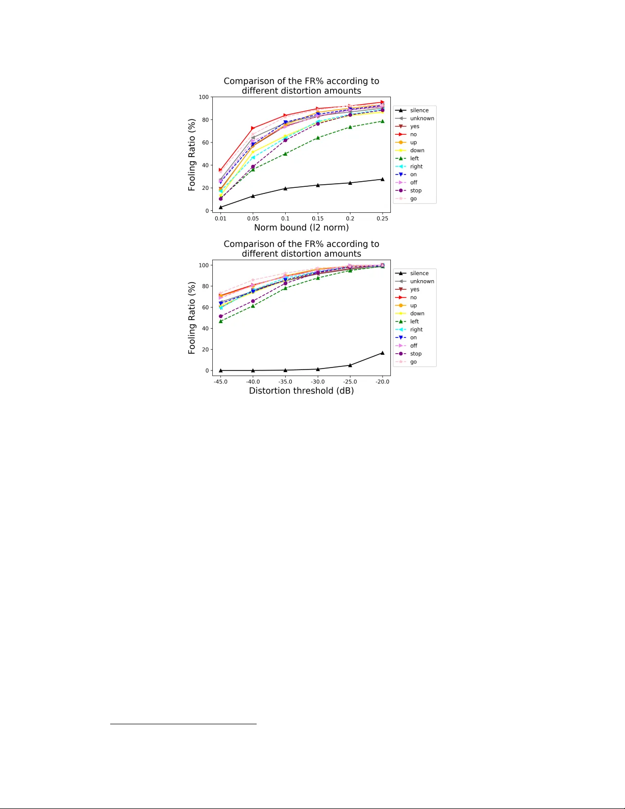
On the human e valuation of audio adv ersarial examples Jon V adillo and Roberto Santana Department of Computer Science and Artificial Intelligence Faculty of Informatics Univ ersity of the Basque Country (UPV/EHU) jvadillo005@ikasle.ehu.eus , roberto.santana@ehu.eus Abstract Human-machine interaction is increasingly dependent on speech communication. Machine Learning models are usually applied to interpret human speech com- mands. Howe v er , these models can be fooled by adversarial e xamples, which are inputs intentionally perturbed to produce a wrong prediction without being noticed. While much research has been focused on de veloping ne w techniques to generate adversarial perturbations, less attention has been gi ven to aspects that determine whether and ho w the perturbations are noticed by humans. This question is rele vant since high fooling rates of proposed adversarial perturbation strategies are only valuable if the perturbations are not detectable. In this paper we in vestigate to which extent the distortion metrics proposed in the literature for audio adv ersarial examples, and which are commonly applied to e valuate the ef fectiv eness of meth- ods for generating these attacks, are a reliable measure of the human perception of the perturbations. Using an analytical frame work, and an experiment in which 18 subjects e valuate audio adversarial examples, we demonstrate that the metrics employed by con vention are not a reliable measure of the perceptual similarity of adversarial e xamples in the audio domain. Keyw ords: Adversarial Examples, Deep Neural Networks, Speech Command Classification, Speech Recognition 1 Introduction Human-computer interaction increasingly relies on Machine Learning (ML) models such as Deep Neural Networks (DNNs) trained from, usually large, datasets [ 1 , 2 , 3 , 4 ]. The ubiquitous applications of DNNs in security-critical tasks, such as face identity recognition [ 5 , 6 ], speaker verification [ 7 , 8 ], voice controlled systems [ 9 , 10 , 11 ] or signal forensics [ 12 , 13 , 14 , 15 ] require a high reliability on these computational models. Howe ver , it has been demonstrated that such models can be fooled by perturbing an input sample with malicious and quasi-imperceptible perturbations. These attacks are known in the literature as adversarial examples [ 16 , 17 ]. Due to the fact that these attacks are designed to be hardly detectable, they suppose a serious concern regarding the reliable application of DNNs in adversarial scenarios. The study of adversarial e xamples has focused primarily on the image domain and computer vision tasks [ 18 ], whereas domains such as text or audio have recei ved much less attention. In fact, such domains imply additional challenges and dif ficulties. One of the evident dif ferences between domains is the way in which the information is represented, and, therefore, the way in which adversarial perturbations are measured, bounded and perceiv ed by human subjects. In the image domain, L p norms are mainly used as a basis to measure the distortion between the original signal and the adversarial example. Howe ver , recent works ha ve pointed out that such metrics do not always Figure 1: Illustration of an adversarial attack, in which an adversarial perturbation is added to a clean audio wa veform, forming an adversarial example which is misclassified by a target DNN model, while not altering the human perception of the audio. properly represent the perceptual distortion introduced by adversarial perturbations [ 19 , 20 , 21 ]. Although in some works L p norms are also used during the generation of adversarial examples to limit the amount of perturbation [ 22 , 23 ], in the audio domain more representative metrics are usually employed for acoustic signals, such as signal-to-noise ratio (SNR) [ 24 , 25 ] or Sound Pressure Lev el (SPL) [ 26 , 27 , 28 ]. These metrics are computed in decibels (dB), which is a standard scale employed for acoustic signals. Ho wever , e ven for such metrics, measuring the perceptual distortion of the attacks is not straightforward, as other characteristics hav e a high influence, such as time- frequency properties. In text problems the dif ficulty of characterizing the perceptual distortion is e ven greater , due to the fact that e very change is inevitably noticeable, and therefore, the aim is to produce semantically and syntactically similar adversarial e xamples [29]. In this paper we focus on the human ev aluation of adversarial examples in the audio domain. A more comprehensiv e approach to ev aluating adversarial distortions can serve to better understand the risks of adversarial attacks in the audio domain. For instance, the dev elopment of adversarial defenses or secure human machine interaction systems can focus on the more effecti ve, unnoticeable, attacks. Therefore, the goal of this study is to perform an analysis of the human perception of audio adversarial perturbations according to dif ferent factors. Based on these results, we will also study to which extent the similarity-metrics emplo yed in the literature are suitable to model such subjecti ve criterion. The remainder of the paper is or ganized as follows: In the following section we introduce the main concepts related to adv ersarial examples and re view previous approaches to e valuate the distortion produced by adversarial perturbation in the audio domain. This section also highlights a number of research questions related to the ev aluation of audio distortion that have not been previously addressed. Section 3 describes the selected task, tar get models and dataset, as well as the particular method employed for generating adversarial perturbation in the audio domain. Section 4 presents a preliminary ev aluation of the adversarial perturbation according to the metrics proposed in the literature. In Section 5, we present the design of an experiment to find answers to some of the issues in volved in the perceptual evaluation of the perturbations. The results of the experiment in which 18 human subjects e valuate dif ferent aspects of the adversarial perturbations are also presented and discussed. Section 6 concludes the paper and identifies lines for future research. 2 Related work The existence of adversarial examples which are able to fool DNNs have been reported for many dif ferent audio related tasks, such as automatic speech recognition [ 22 , 30 , 31 ], music content analysis [ 32 ] or sound classification [ 28 ]. A common adversarial attack scheme is represented in Fig. 1. Note that it is assumed that an adversary can feed the perturbed signal directly into the model. Even if this is a common assumption, some works ha ve demonstrated that such attacks can be designed to work in the physical world [24, 33, 34]. Our work builds on pre vious research where adversarial perturbations for audio command classifica- tion hav e been introduced [ 35 ]. Ho wever , the e valuation methods and type of analysis presented in this paper are valid for other approaches concei ved to generate audio adversarial e xamples for other ML tasks. 2 2.1 Adversarial example: formal description Let f ( x ) be a classification model f : X → Y , which classifies an input x from the input space X as one of the classes represented in Y = { y 1 , ..., y k } . An adversarial example x 0 is defined as x 0 = x + v , where v ∈ R d represents the adversarial perturbation capable of producing a misclassification of f for the (correctly classified) input x : f ( x ) 6 = f ( x 0 ) . A necessary requirement for an adversarial attack is that the perturbation should be imperceptible , and therefore, the goal is to minimize the distortion introduced by v as much as possible, according to a suitable distortion metric ϕ ( x, x 0 ) → R Depending on the objective of the attack, adversarial examples can be categorized in different ways. First of all, a tar geted adversarial e xample consists of a perturbed sample x 0 = x + v which satisfies f ( x 0 ) = t , where t represents the target (incorrect) label that we want to be produced by the model. In contrast, an untar geted adversarial e xample only requires the output label to be incorrect f ( x 0 ) 6 = f ( x ) , without any additional re gard about the output class assigned to x 0 . Furthermore, depending on the scope of the adversarial perturbation v , we can differentiate between individual or universal adv ersarial perturbations. In the first case, the perturbation is crafted specifi- cally to be applied to one particular input x . Therefore, it is not expected that the same perturbation will be able to fool the model for a different sample. In the second case, univ ersal adversarial examples are input agnostic perturbations able to fool the model independently of the input. In [ 35 ], different lev els of univ ersality are proposed, depending on the number of classes for which it is expected to work. The first uni versality lev el comprises single-class universal perturbations that are concei ved to fool the target model only for inputs of one particular class. W e will focus on single-class univ ersal perturbations, although our findings regarding the weaknesses and gaps in the ev aluation of adversarial perturbations are not restricted to this uni versality le vel. 2.2 Methods for assessing audio adv ersarial perturbations In this section we collect the strategies employed by previous works in order to verify that audio perturbations are not detectable by humans. Even if an essential requirement for adversarial perturba- tions to suppose a real threat is that they must be imperceptible, a good specification of such (mainly subjectiv e) a constraint is not straightforward, and, indeed, is not well established yet. Furthermore, ev en if the analysis is constrained to the audio domain, the understanding and definition of what can make a sample natural is very related to the ML task that is being solved by the model (e.g., it might be harder to categorize a music tune as “unnatural” than a spoken command). W ith a large v ariety of ML tasks related to the analysis of acoustic signals (e.g., speech recognition, music content analysis or ambient sound classification), each of them may require, therefore, a different criterion to assess the distortion of the adversarial examples according to human perception. Although a number of strategies ha ve been proposed in these domains [ 27 , 32 , 26 , 36 , 30 ], we focus on those suitable for spoken commands. Among these strategies are: • Thresholding the perturbation amount • Models of human perception and hearing system • Human e valuation 2.2.1 Thresholding the perturbation amount The methods discussed in this section rely on limiting or measuring the perturbation amount that is added to the original input, according to a distortion metric, to ensure that the perturbations are imperceptible or quasi-imper ceptible , or that the distortion levels are belo w a maximum acceptable threshold. In [ 22 ], the perturbation applied to spoken commands is restricted to the 8 least-significant-bits of a subset of samples in a 16 bits-per-sample audio file. Similarly , in [ 23 ], the effecti veness of the proposed attack for speech paralinguistic tasks is measured for different perturbation amounts under the ` ∞ norm. The restrictions applied in both cases guarantee that the maximum change applicable to each value of the signal is constrained. Howe ver , such thresholds are not representative for acoustic signals, as they do not guarantee a lo w perceptual distortion on audio attacks. In [ 30 , 31 , 37 ], in which audio adversarial perturbations for speech recognition models are addressed, the relati ve loudness of the adv ersarial perturbation v with respect to the original signal x is measured 3 in Decibels (dB), which is a more representativ e metric for acoustic signals: dB x,max ( v ) = dB max ( v ) − dB max ( x ) , (1) where dB max ( x ) = max i 20 log 10 ( x i ) (2) In [ 25 ], the signal to noise ratio (SNR) is used to measure the relativ e distortion of adversarial perturbations for speech recognition models, computed as: S N R ( x, v ) = 10 log 10 P ( x ) P ( v ) , (3) where P ( x ) and P ( v ) represent the power of the clean signal x and the perturbation v , respectiv ely . The SNR has been used in other works on audio adversarial examples [ 32 , 33 , 34 , 24 , 28 ]. Howe ver , these works are not based on speech signals, as their approaches rely on data with very different characteristics, such as urban sound classification, music content analysis or the injection of malicious commands into songs. Therefore, the results are not directly comparable to spoken speech recognition, the tasks addressed in this paper . 2.2.2 Models of human perception and hearing system The human hearing system is able to identify sounds in a range from 20Hz to 20kHz, so that perturbations outside this range can not be percei ved [ 38 , 39 ]. Based on this fact, in [ 26 ] and [ 27 ], high frequencies are used to generate audio inaudible to humans but which is captured and classified by a de vice. Although these attacks may not fit in our specification of adv ersarial examples (since humans cannot perceive the generated audio, and therefore cannot judge it as benign either), they introduce the idea of using frequenc y ranges that are out of the human hearing range in adv ersarial scenarios. A dif ferent strategy is employed in [ 36 ], where a psychoacoustic model [ 40 ] is used to compute the hearing thresholds of different zones of the clean audio signal, which is used to restrict the perturbation to the least perceptible parts. 2.2.3 Human evaluation In [ 41 ] and [ 42 ], an ABX test is performed, which is a standard method to identify detectable differences between tw o choices of sensory stimuli. In this method a subject is asked to listen to two audios A and B, and afterwards a third audio X, which will be either A or B, randomly selected. The objectiv e of this test is to assess if the user is able to distinguish between A and B. Optimally , the accuracy ratio would be 50%, equal to the probability of selecting randomly between the two choices. In our scenario, the two initial audios A and B would correspond to the clean and perturbed audio (in any order). In [ 24 ] and [ 34 ] the adversarial perturbations are embeded in songs, which can be deplo yed in the physical world without raising suspicions for humans listeners (e.g., in ele vators or TV advertisements) to force a target model to understand speech commands. In both works a human ev aluation is carried out on Amazon Mechanical T urk. According to the results presented by the authors, almost none of the participants perceived speech in the perturbed signals. Howe ver , a considerable percentage of people reported that an abnormal noise could be noticed in the songs. In [ 36 ], a Multiple Stimuli with Hidden Reference and Anc hor (MUSHRA) test is carried out [ 43 ], to perform a subjectiv e assessment of the audio quality of adversarial examples. The goal of the test is to score the quality of perturbed audio signals ( anc hors , e.g., adversarial examples) with respect to the original signal ( hidden r efer ence , in this context, the original audio). 1 According to the results, the adversarial e xamples obtained considerably lower scores than the clean audio signals. Finally , in [ 44 , 33 , 22 , 23 , 25 ], experiments with human subjects are performed with the aim of analyzing their response to the task, in order to assess if the adversarial perturbation has an y influence on the responses provided by human listeners. Ho wever , no analysis of the perceptual distortion introduced by the perturbations is reported, except in [ 25 ], in which the subjects are asked to e valuate the noise lev el of the audio signals. 1 It is w orth mentioning that this test is mainly used to assess the intermediate quality le vel of coding systems, whereas for small impairments, which should be the case of audio adversarial perturbations, dedicated tests have been proposed. 4 2.3 Summary Despite the f act that dif f erent methods have been proposed to measure the distortion levels introduced by audio adversarial perturbations, we found that the majority of the approaches are not enough to adequately represent the human perception of these attacks. Apart from that, some of the thresholds and acceptable distortion lev els assumed in previous works do not alw ays guarantee that the perturba- tions are imperceptible, and therefore, the detectability of the attacks can be questionable. W ith this paper , we intend to provide e vidence and raise awareness about these g aps. W e hope that the results reported may contribute to establish a more thorough measurement of the distortion, and therefore, to a more realistic study of audio adversarial e xamples. 3 Adversarial examples of speech commands Our goal is to e valuate the detectability of audio adv ersarial perturbation, and to determine to what extent the metrics commonly used in the literature agree with the human e valuation. T o accomplish this goal, we should first establish a number of stepping stones: 1. Identify a suitable and representati ve audio task. 2. Identify a model appropriate for the task 3. Collect or identify a dataset to train a model. 4. Using the model, generate the adv ersarial examples for the task. 5. Estimate the actual fooling rate of the adv ersarial examples. 3.1 Selection of the task, model, and dataset The task we have selected is speech command classification since it is an exemplar machine learning task which is part of the repertoire of extensi vely used speech-based virtual assistants. The DNN model we have selected is based on the architecture proposed for small-footprint keyw ord recognition [ 45 ]. This model takes as input an audio wav eform, computes the spectrogram of the signal and extracts a set of MFCC features for different time intervals. This results in a two- dimensional representation of the audio signal, which is fed into the following topology: two con volutional layers with a ReLU acti vation function, a fully-connected layer and a softmax layer . The same architecture has been used in related works on adversarial examples [ 22 , 25 ] and as a baseline model in other research tasks [46, 47]. W e used the Speech Command Dataset [ 46 ], which is a widely used dataset in the study of adversarial attacks for speech recognition systems [ 22 , 37 , 25 ]. The dataset is composed of recordings of 30 different spok en commands, provided by a large number of different people. Audio files are stored in a 16-bit W A V file, with a sample-rate of 16kHz and a fixed duration of one second. As in previous publications [ 46 , 22 ], we selected the following subset of commands to dev elop our work: “Y es”, “No”, “Up”, “Do wn”, “Left”, “Right”, “On”, “Off ”, “Stop”, and “Go”. Additionally , W e will also consider two special classes: “Unknown” (a spoken command not considered in the pre vious set), and “Silence” (no speech detected in the audio). Note that this selection comprises a wide variety of commands in terms of phonetic similarity . 3.2 Generating single-class universal perturbations As pre viously mentioned, we focus on single-class uni versal perturbations, an attack approach that attempts to generate a single perturbation which is able to fool the model for any input corresponding to a particular class y . W e decided to focus on univ ersal perturbations because an initial experimenta- tion with indi vidual perturbations (crafted using Deepfool algorithm) led us to the conclusion that the perturbations were undoubtedly imperceptible. This conclusion has been reported before in the literature [ 19 ] for the case of image adversarial examples. Therefore, we selected the more challeng- ing task of generating uni versal perturbations, which requires higher distortion le vels. Moreo ver , we selected single-class univ ersal attacks in order to study in more detail the results on different commands. The particular choice of the class to which the tar get perturbation is applied is a factor that may influence the perceptual distortion of the perturbations. 5 T able 1: Effecti veness of the generated single-class uni versal perturbations. Class Max. FR% Mean FR% T rain V alid T rain V alid Silence 23.80 19.46 22.24 19.61 Unknown 72.70 73.06 70.58 73.51 Y es 74.50 74.36 68.26 66.40 No 86.50 83.77 81.48 79.40 Up 84.20 75.45 82.20 74.73 Down 71.50 65.55 68.06 64.51 Left 52.30 49.73 42.20 40.59 Right 68.70 63.82 60.62 56.47 On 76.00 75.65 54.42 53.28 Off 80.10 73.48 75.18 70.85 Stop 61.40 61.82 56.92 57.30 Go 87.80 80.06 86.24 80.90 The selected attack method is based on the strategy proposed in [ 48 ], a state-of-the-art method to generate univ ersal perturbations based on accumulating individual perturbations created for a set of training samples using the Deepfool algorithm [ 49 ]. W e use the U AP-HC reformulation of this strategy for audio samples as presented in [ 35 ], where more details about the process to generate the perturbations can be found. W e generated 5 different uni versal perturbations per class, starting from a different training set of 1000 samples in each case. During the crafting process, the univ ersal perturbations were bounded by the ` 2 norm, with a threshold value of ξ = 0 . 1 . In addition, the Deepfool algorithm was limited to a maximum number of 100 iterations. The overshoot parameter of the Deepfool algorithm w as set to 0.1. Finally , the U AP-HC algorithm was restricted to 5 epochs, that is, 5 complete passes through the entire training set. 3.3 Effectiveness of the perturbations f ooling the model T o measure the effecti veness of the univ ersal perturbations, we compute the percentage of audios for which the prediction changes when the perturbation is applied. W e will refer to this metric as fooling ratio (FR) [ 48 ]. The effecti veness of the generated perturbations is shown in T able 1, for the training set (the set of samples used to optimize the univ ersal perturbation) and for the validation set (the set of samples used to compute the effecti veness of the attack for inputs not used during the optimization process). 2 Results are shown for the a verage ef fectiveness of the 5 perturbations generated for each class, as well as for the one that maximizes the FR on the training set. According to the results, the generated adversarial e xamples are highly effecti ve for the majority of the classes, with a maximum FR abo ve 70% for 7 out of 12 classes in both training and validation sets. Note that we obtain a considerably high effecti veness also in the class unknown , which is composed of a di verse set of spoken commands. Howe ver , the hardest class to fool is silence , in which the maximum FR is below 25% in both training and validation sets. This may be due to the fact that, according to the nature of the audios corresponding to that class, trying to fool the model by adding a small amount of noise is a challenging task. It is important to bear in mind that the effecti veness of a univ ersal perturbation is directly correlated to the distortion amount introduced. W e show in Fig. 2, for each class, the way in which the FR increases as the distortion amount introduced by the perturbations increases. These results hav e been obtained by scaling the magnitude of a uni versal perturbation v according to two distortion criteria: the ` 2 norm of the perturbation and the decibel difference between the perturbation and each sample of the dataset. In the first case, the perturbation signal is scaled in order to ensure that its norm equals the desired threshold, and it is equally applied to e very input sample. In the second case, the 2 The samples used to optimize the perturbation will be selected from the training set used to train the DNN. Equiv alently , the validation set of the algorithm will be selected from the validation set used during the training process of the model. 6 Figure 2: V ariation in the effecti veness (FR%) in the validation set of the generated single-class univ ersal adversarial perturbations according to two dif ferent criteria: ` 2 norm of the perturbation (top) and dB x,max ( v ) metric with respect to each input signal x (bottom). perturbation signal is scaled for ev ery input sample x , in order to ensure that the dB x,max ( v ) metric equals the specified threshold. The fact that the FR is directly correlated with the distortion lev el implies that there is a trade-off between the effecti veness and the detectability of the attacks. Therefore, to adequately study the risk posed by audio adversarial attacks, it is important to establish realistic and rigorous criteria for assessing the human perception of such attacks. 4 Evaluation of the distortion using similarity metrics While the ability to fool the model is an essential ingredient of adversarial examples, the other requirement is that the perturbation is not noticed by humans. In this section, we ev aluate the distortion produced by the generated adversarial perturbations, according to dif ferent criteria. 4.1 Evaluating the distortion: the standard, uninformed way W e first computed the distortion according to the standard approaches employed in pre vious works on adversarial e xamples in speech related tasks [ 30 , 31 , 37 ], as described in equation (1) (Section 2.2). In [ 30 ], where individual adv ersarial perturbations are created for speech transcription scenarios, the mean distortion of the generated perturbations is -31dB, and the 95% interv al for distortion ranges from -15dB to -45dB. 3 The same range of distortion is reported in [ 37 ]. In [ 31 ], where universal adversarial perturbations are generated also for speech transcription models, the distortion le vel of 3 Note that according to this metric, the lower the distortion v alue, the less detectable the perturbation. 7 T able 2: Distortion le vels produced by the generated single-class uni versal perturbations (standard ev aluation). Results are av eraged for the 5 experiments carried out for each class. Class Mean dB x,max ( v ) % of samples below -32dB Silence -29.52 48.04 Unknown -41.35 90.20 Y es -40.58 90.45 No -42.56 93.09 Up -40.24 89.18 Down -40.63 90.64 Left -48.10 99.03 Right -43.30 95.20 On -46.31 96.21 Off -42.01 94.03 Stop -43.92 96.11 Go -41.88 93.28 the perturbations is bounded under different thresholds, obtaining a mean distortion of ≈ − 42 dB in the best case, and a mean distortion of ≈ − 30 dB in the worst case. Overall, distortion le vels belo w -32dB are considered acceptable in these works. Fig. 3 sho ws the distortion lev el of the generated perturbation with respect to each input sample in the validation set, according to the same approach. Results are computed independently for each class, and averaged for the 5 trials carried out in each of them. T able 2 shows the mean distortion lev el obtained for each class. As can be seen, the mean distortion is belo w -40dB in all the classes except silence , in which the mean distortion is of -29.52dB 4 . Moreover , without considering the class silence , more than 90% of the samples are below -32dB in all the cases. Therefore, our perturbations can be considered as highly acceptable according to this standard. Figure 3: Distortion lev el of the generated single-class univ ersal perturbations, ev aluated in the validation set using the standard ev aluation approach: dB x,max ( v ) applied to the whole signals. Results are av eraged for the 5 perturbations generated for each class. 4.2 Evaluating the distortion: detailed and signal-part-informed way In order to measure the distortion in more detail, we employed the approach presented in [ 35 ]. In this case, the distortion induced by the perturbation v in the original sample x is computed in terms of 4 This effect can be e xplained by the fact that, due to the nature of the samples corresponding to the class silence , their loudness lev el is lower than for the rest of classes. 8 the difference between both the maximum (as defined in equation (1) ) and the mean decibel values, defined as: dB x,mean ( v ) = dB mean ( v ) − dB mean ( x ) , (4) where dB mean ( x ) = 20 · log 1 d d X i =1 | x i | ! (5) Furthermore, previous work on ev aluating the naturalness of adversarial examples in the audio domain compute the distortion between two signals by applying the metrics to the entire signals [ 30 , 37 , 31 ]. In this paper , we advocate the application of both metrics in two different parts of each audio signal: the vocal part and the bac kground part. This dif ferentiation is due to the fact that, for spoken commands, the amount of sound outside the vocal part is considerably lower . Thus, the same amount of perturbation would be percei ved differently depending on the infected part. By mapping the distorti ve effect of the perturbations to these parts of the signals we also get a better assessment of how the attack w orks better . As we are handling short single-command audio signals, the vocal part of an audio signal x = { x 1 ...x d } will be delimited by the continuous range [ x a , x b ] containing 95% of the energy of the signal, that is: P b i = a x 2 i P d i =1 x 2 i ≈ 0 . 95 . (6) Thus, we will assume that ranges [ x 1 , x a ) ∪ ( x b , x d ] will be composed just of background noise. Notice that this partition is well suited for single command audios in which it is assumed that the vocal part of the signal is contiguous. Audio signals belonging to the silence class will be omitted from the analysis of the vocal part, as they are composed only of background noise, without any vocal part. 4.3 Results of the different signal-part appr oach The results obtained with the described ev aluation approach are shown in Fig. 4. The first row of the figure shows the results obtained using dB x,max ( v ) metric, and the bottom row the results obtained using dB x,mean ( v ) metric. Notice the difference between the horizontal axis scales of the figures. By comparing the perturbations in the vocal part and the background part, it can be seen that perturbations in the vocal part are less noticeable, with a decibel dif ference significantly lower , which occurs using both dB max and dB mean distortion metrics. Regarding the distortion amount in the vocal part, the obtained results are significantly below the threshold of − 32 dB in almost all the samples, independently of the metric. Compared to the sound intensity le vel of a normal con versation, a distortion of − 30 dB corresponds to the weakest audible signal between 10kHz and 100Hz frequency range [ 50 ], which is roughly the difference between the ambient noise in a quiet room and a person talking [30]. While the distortion lev el outside the vocal part is still acceptable under the dB max metric, according to the dB mean metric the distortion exceeds the threshold of -32dB for a great majority of the samples. In fact, in about half of the cases the difference in decibels is greater than -20dB, which may indicate that the perturbations could be highly detectable in those parts. 5 Human ev aluation of voice command adversarial examples While the methods presented in the previous section provide a more accurate and detailed assessment on the quality of the adversarial examples, the metrics used are not expected to capture all the subtleties of a proper human e valuation. Therefore, we designed an experiment in which human subjects listen to audio adversarial examples and judge them according to dif ferent criteria. The main goal of the experiment w as to study to which extent the perturbations are detectable by humans. In this section we describe the experimental design and its results. 9 Figure 4: Distortion lev el of the generated single-class univ ersal perturbations, ev aluated in the validation set using dB x,max ( v ) metric (top ro w) and dB x,mean ( v ) metric (bottom ro w). For each audio, the distortion has been measured in the v ocal part as well as in the background part. Results are av eraged for the 5 perturbations generated for each class. 5.1 Experimental design A set of eighteen subjects (12 men and 6 women), independent of the research, was selected to conduct the experiment. Each participant was instructed to listen to dif ferent audio clips and answer some questions about them. The experiment is composed of two parts: • In the first part, the naturalness of the generated universal adversarial examples is in vestigated. The other question in vestigated is to what extent the distortion produced by the perturbation affects the understandability of the spoken commands. T o address these questions, the participants are asked to listen a set of 12 audio clips, either clean or adv ersarially perturbed, and provide the follo wing information: – Identify the command that can be heard in the audio clip, in order to determine if the adversarial perturbations af fect the understandability of the spoken commands. – Assess the lev el of naturalness of the audio clip, in order to study whether the adversarial examples are percei ved as perturbed audios in comparison to clean instances. As both clean and perturbed audios will be tested, the comparison between the results obtained in both cases may reflect if the perturbations are perceiv ed just as a regular background noise or other ordinary perturbations, or whether they are perceived as artificial or malicious. In the experiment, the subjects e valuated the naturalness on a scale from 1 to 5, with the following scale pro vided as reference: 1) Clearly perturbed audio with an artificial sound or noise. 2) The audio is slightly perturbed by an artificial sound or noise, not likely to be caused by the low quality of the microphones or ambient sounds. 3) Not sure 4) No obvious signs of an artificial perturbation. The detectable perturbations are likely to be caused by a low- or mid-quality microphone, ambient sounds or ordinary noises. 5) The audio clip clearly does not contain any artificial perturbation. 10 • In the second part of the experiment, each participant performed an ABX test, a method to identify detectable dif ferences between two choices of sensory stimuli. In this method, a subject is asked to listen to two audios A and B, and afterwards a third audio X, which will be either A or B, randomly selected. The goal of the test is to ev aluate if the subject is able to determine if X corresponds to A or to B. In our experiment, the two initial audios A and B will correspond to the clean and perturbed audio, in any order . Thus, this test will determine if the perturbations are detectable in comparison to the clean audio sample. Six trials were carried out in each experiment, that is, six sets of three audio clips A, B and X. Due to the f act that the audio clips of the dataset contain dif f erent characteristics, such as the intensity of the spoken command or the amount of background noise, the perception of a perturbation may change according to these features. For this reason, we decided to classify the audios considering three lev els of intensity: low , medium and high. The dB mean distortion metric presented in (5) will be used to measure the mean distortion of the audio signals. According to this metric, 99% of the intensities of the audio samples lie approximately in the decibel range [30 , 85] . By performing a rough uniform binning of the intensity range (kno wn as equal-width binning in the literature [ 51 ]), the lev els were defined as follows: • Lo w intensity lev el: audios with a mean distortion below 50dB. • Medium intensity le vel: audios with a mean distortion between 50dB and 70dB. • High intensity le vel: audios with a mean distortion above 70dB. T o ensure a uniform representation of the different le vels of intensity , each experiment was composed of audio signals of only one of these lev els. Nine different e xperiments were created, (three exper - iments per intensity lev el), and each of them was assigned to two different participants, making a total of 18 e xperiments and participants. A summary of the final e xperimental setup is provided in T able 3. The minor unbalance in the number of original and modified audios in the first part of the experiment is assumed to ensure greater uniformity in the frequency of each command, depending on the different factors influencing the experiment, as shown in T able 4, as well as to ensure that the model correctly classified the original audio samples but incorrectly classified the adversarial examples. 5.2 Analysis of the results 5.2.1 Command classification task The first factor to be analyzed is the accuracy percentage obtained by humans in the command classification task (first part of the experiment), that is, which percentage of samples hav e been correctly labeled by humans. According to the results, the total number of instances wrongly classified considering all the instances, clean and adversarial, is 13 out of 216 (9 corresponding to clean samples and 4 to adversarial samples), which corresponds to a total accurac y in the command classification of ∼ 94 %. In order T able 3: Summary of the experimental setup designed for the human ev aluation of the distortion produced by the univ ersal perturbations. Experiment Intensity Audio samples (part 1) ABX trials (part 2) Clean Adv . T otal 1 Low 6 6 12 6 2 Low 6 6 12 6 3 Low 5 7 12 6 4 Medium 6 6 12 6 5 Medium 6 6 12 6 6 Medium 7 5 12 6 7 High 6 6 12 6 8 High 6 6 12 6 9 High 7 5 12 6 11 T able 4: Number of audios per command used in the experiment (part 1). T ype Sil. Unk. Y es No Up Down Left Right On Of f Stop Go Low intensity 6 6 6 6 6 6 6 4 6 6 8 6 Medium intensity 6 4 8 6 6 6 6 6 6 6 6 6 High intensity 6 12 8 6 0 12 4 8 2 2 4 8 Clean 12 2 8 12 4 22 12 4 4 12 14 4 Adversarial 6 20 14 6 8 2 4 14 10 2 4 16 T otal Frequency 18 22 22 18 12 24 16 18 14 14 18 20 to provide more detailed information, the accuracies obtained for each intensity le vel are sho wn in Fig. 5, in which the percentages are computed independently for clean instances and for adversarial examples. Overall, these results indicate that the adversarially perturbed spoken commands are clearly recognizable and well classified by humans, independently of the intensity level of the original audio. In other words, although the adversarial perturbations are able to fool the tar get model, they do not affect the human understanding of the command. The obtained results are consistent with those achiev ed in [ 25 ], where the success rate of a set of people in classifying audio commands is reported using the same dataset as us, but without considering silence or unknown as classes and without differentiating between the intensity le vel of the original signals. According to the results reported in [ 25 ], the accuracy in recognizing the commands was 93.5% for clean samples and 92.0% for adversarial e xamples. Figure 5: Accuracy percentages achieved by the participants of the experiment in the speech command classification task. Results ha ve been split for each sample type (clean or adversarial) as well as for the intensity lev els of the original audios in the experiments (lo w , medium or high). 5.2.2 Naturalness Furthermore, the results obtained in the analysis of the naturalness lev el assigned to the instances is displayed in Fig. 6. The figure shows the frequencies with which samples are classified in each naturalness lev el, split according to the sample type (clean or adversarial). In addition, the results are jointly computed for all the experiments (top left) as well as for each intensity lev el individually: low (top right), medium (bottom left) and high (bottom right). Considering all the experiments, it can be observed that the adversarial examples obtained lower scores in comparison to the clean samples. W e verified by an e xact multinomial statistical test that there exist significant dif ferences regarding the scores assigned to clean and adv ersarial audios (achieving a p-value belo w a tolerance of 0 . 01 ). Indeed, while 65 . 5 % of the clean samples are classified with a naturalness lev el of 4 or 5, only 33 % of adversarial e xamples hav e been classified in the same range. These results indicate that, in general, the adversarial perturbations are percei ved in the audio signals as artificial sounds or noises with a considerably higher frequency than clean samples. Doing the same analysis independently for each intensity lev el, it can be observed that the main difference is gi ven in the lowest intensity le vel, in which 86 . 9 % of the adversarial examples achie ved a score of 1 or 2 , while only 14 . 7 % of clean samples were classified in that range. For the highest 12 intensity le vel, ho wev er, the percentage of adv ersarial examples scored with a 4 or 5 is e ven greater than the corresponding percentage for clean samples. Thus, the human perception of the adversarial examples is clearly related to the intensity le vel of the original audio signals. This is a remarkable fact that should be taken into consideration in the e valuation of audio adv ersarial examples. Figure 6: Analysis of the naturalness lev el assigned to the audio samples of the speech command classification task in all the experiments, split by sample type (clean or adversarial). The results are computed for all the experiments (top left) as well as for each intensity le vel individually: low (top right), medium (bottom left) and high (bottom right). 5.2.3 ABX test In order to better e valuate if the perturbations are percei vable, the results obtained in the ABX test (second part of the e xperiment) ha ve been analyzed. This is summarized in Fig. 7. The first ro w of the figure sho ws the percentage of success cases in the ABX test, that is, the percentage of cases in which the unknown audio (audio X) has been correctly classified. The second row shows the confidence lev el of the answers. All these results have been computed independently for each intensity le vel. The success rate of the experiments with low and medium intensity levels is of 97 . 2 % and 91 . 7 % respectiv ely , re vealing that the perturbations are clearly percei vable in such cases. On the contrary , only a 55 . 6 % success rate is achie ved for high intensity le vels, close to the optimum v alue of 50 %, which is equi valent to a random guessing. W e verified by an exact binomial test 5 that the achie ved success ratio is no significantly greater (achie ving a p-value of ≈ 0 . 31 ) than the probability p = 0 . 5 corresponding to a binomial distribution X ∼ B ( n = 36 , p = 0 . 5) , where n is the sample size. This fact indicates that, in such cases, the adversarial examples are not distinguishable from their corresponding clean audio examples. It is worth noting that, given our experimental setup, 95% (Clopper–Pearson) confidence interv als of the success ratio is [0 . 85 , 0 . 99] for lo w intensity audios, [0 . 78 , 0 . 98] for medium intensity audios and [0 . 38 , 0 . 72] for high intensity audios. The results provided can, therefore, be considered representati ve of the human perception of the distortion. Consistently with the success rates, the subjects were highly confident in providing their answers in more than 75 % of the cases in the experiments containing audios with lo w and medium intensity le vels. Contrarily , in 75 % of the answers the participants reported a lo w confidence in the experiments containing audios with high intensity lev els. 5 The alternativ e hypothesis of the test is that the empirical success ratio is greater than p = 0 . 5 . The same test with the alternativ e hypothesis that the empirical ratio is not equal to 0 . 5 obtained a p-value of ≈ 0 . 62 . 13 Overall, these analyses demonstrate that the detectability of the perturbations largely depends on the intensity lev el of the clean audio, being detectable for audios with low and medium intensity le vels, but not percei vable for audios with a high intensity le vel. It is worth mentioning that, according to the standard approach used in previous related works to measure the detectability of audio adversarial examples, the crafted perturbations were far below the maximum acceptable distortion. Howe ver , the results obtained in this section reinforce our proposal about the need to employ more rigorous approaches in order to measure and set a threshold on the distortion produced by the adversarial perturbations in a more representativ e way . W e encourage the reader to listen to some adv ersarial examples, to empirically assess the perceptual distortion of adversarial perturbations according to dif ferent characteristics. 6 Figure 7: Success percentages obtained in the ABX test (top) and confidence lev els of the answers in the test (bottom), both computed independently for each intensity lev el. 6 Conclusions In this paper we ha ve addressed the measurement of the perceptual distortion of audio adversarial examples, which remains a challenging task despite being a fundamental condition for effecti ve adversarial attacks. For this purpose, we ha ve performed an analysis of the human perception of audio adversarial perturbations for speech command classification tasks, and this analysis has been used to study whether the distortion metrics employed in the literature correlate with the human judgment. W e hav e found out that, while the distortion le vels of our perturbations are acceptable according to the standard ev aluation approaches employed by con vention, the same perturbations were highly detectable and judged as artificial by human subjects. F or this reason, we have proposed a novel framew ork to measure the distortion in a more comprehensi ve way , based on a dif ferential analysis in the vocal and background parts of the audio signals, which provide a more realistic and rigorous ev aluation of the perceptual distortion. Our experiments with single-class univ ersal perturbations for a set of varied commands also demonstrate that there exist dif ferences regarding the ef fectiveness of the attacks, related to the relati ve distortion, and ho w the perceptual distortion of the perturbations changes depending on the intensity lev els of the audio signal in which it is injected. 6 https://vadel.github.io/adversarialDistortion/AdversarialPerturbations.html 14 These results highlight the lack of audio metrics capable of modeling the human perception in a realistic and representative way , and stress the need to include human ev aluation as a necessary step for v alidating methods used to generate adversarial perturbation in the audio domain. W e hope that future works could adv ance in this direction in order to fairly e valuate the risk that adversarial examples suppose. Acknowledgments The authors would like to thank to the Intelligent Systems Group (Uni versity of the Basque Country , Spain) for providing the computational resources needed to dev elop the project. This work has receiv ed support form the predoctoral grant that Jon V adillo holds by the Basque Government (reference PRE_2019_1_0128). Roberto Santana acknowledges support by the Basque Go vernment (IT1244-19 and ELKAR TEK programs), and Spanish Ministry of Economy and Competitiveness MINECO (project TIN2016-78365-R). References [1] Bin Fang, Fuchun Sun, Huaping Liu, and Chunfang Liu. 3D human gesture capturing and recognition by the IMMU-based data glov e. Neur ocomputing , 277:198–207, 2018. [2] Jianfeng Gao, Michel Galle y , Lihong Li, et al. Neural approaches to conv ersational AI. F oundations and T r ends® in Information Retrieval , 13(2-3):127–298, 2019. [3] Mohammed Mehedi Hassan, Md Zia Uddin, Amr Mohamed, and Ahmad Almogren. A robust human activity recognition system using smartphone sensors and deep learning. Futur e Generation Computer Systems , 81:307–313, 2018. [4] Juan C Nunez, Raul Cabido, Juan J P antrigo, Antonio S Montemayor , and Jose F V elez. Conv olutional neu- ral networks and long short-term memory for skeleton-based human activity and hand gesture recognition. P attern Recognition , 76:80–94, 2018. [5] Y i Sun, Y uheng Chen, Xiaogang W ang, and Xiaoou T ang. Deep learning face representation by joint identification-verification. In Advances in neural information pr ocessing systems , pages 1988–1996, 2014. [6] Omkar M Parkhi, Andrea V edaldi, Andre w Zisserman, et al. Deep face recognition. In BMVC , volume 1, page 6, 2015. [7] Georg Heigold, Ignacio Moreno, Samy Bengio, and Noam Shazeer . End-to-end text-dependent speaker verification. In 2016 IEEE International Conference on Acoustics, Speech and Signal Pr ocessing (ICASSP) , pages 5115–5119. IEEE, 2016. [8] David Snyder , Daniel Garcia-Romero, Daniel Pove y , and Sanjeev Khudanpur . Deep neural network embeddings for text-independent speaker v erification. In Interspeech , pages 999–1003, 2017. [9] Huan Feng, Kassem Fawaz, and Kang G Shin. Continuous authentication for voice assistants. In Pr oceedings of the 23r d Annual International Conference on Mobile Computing and Networking , pages 343–355. A CM, 2017. [10] Andrew Boles and P aul Rad. V oice biometrics: Deep learning-based voiceprint authentication system. In 12th System of Systems Engineering Confer ence (SoSE) , pages 1–6. IEEE, 2017. [11] Y uan Gong and Christian Poellabauer . An overvie w of vulnerabilities of voice controlled systems. arXiv pr eprint arXiv:1803.09156 , 2018. [12] Belhassen Bayar and Matthew C Stamm. Constrained conv olutional neural networks: A new approach tow ards general purpose image manipulation detection. IEEE T ransactions on Information F or ensics and Security , 13(11):2691–2706, 2018. [13] Belhassen Bayar and Matthew C Stamm. A generic approach tow ards image manipulation parameter estimation using con volutional neural networks. In Pr oceedings of the 5th ACM W orkshop on Information Hiding and Multimedia Security , pages 147–157. A CM, 2017. [14] Jinhua Zeng, Jinfeng Zeng, and Xiulian Qiu. Deep learning based forensic face verification in videos. In 2017 International Confer ence on Pr ogress in Informatics and Computing (PIC) , pages 77–80. IEEE, 2017. 15 [15] MS Athulya, PS Sathidevi, et al. Mitigating effects of noise in forensic speaker recognition. In 2017 International Confer ence on W ireless Communications, Signal Pr ocessing and Networking (W iSPNET) , pages 1602–1606. IEEE, 2017. [16] Christian Szegedy , W ojciech Zaremba, Ilya Sutske ver , Joan Bruna, Dumitru Erhan, Ian Goodfellow , and Rob Fergus. Intriguing properties of neural networks. In 2nd International Confer ence on Learning Repr esentations , pages 1–10, 2014. [17] Ian J Goodfellow , Jonathon Shlens, and Christian Sze gedy . Explaining and harnessing adv ersarial examples. arXiv pr eprint arXiv:1412.6572 , 2014. [18] Nav eed Akhtar and Ajmal Mian. Threat of adversarial attacks on deep learning in computer vision: A surve y . IEEE Access , 6:14410–14430, 2018. [19] Sid Ahmed Fezza, Y assine Bakhti, W assim Hamidouche, and Olivier Défor ges. Perceptual ev aluation of adversarial attacks for CNN-based image classification. In 2019 Eleventh International Conference on Quality of Multimedia Experience (QoMEX) , pages 1–6. IEEE, 2019. [20] Matt Jordan, Naren Manoj, Surbhi Goel, and Alexandros G Dimakis. Quantifying perceptual distortion of adversarial e xamples. arXiv preprint , 2019. [21] Y onatan Dukler, W uchen Li, Alex T ong Lin, and Guido Montúfar . W asserstein of W asserstein loss for learning generativ e models. 2019. [22] Moustafa Alzantot, Bharathan Balaji, and Mani Sriv astav a. Did you hear that? Adversarial examples against automatic speech recognition. arXiv preprint , 2018. [23] Y uan Gong and Christian Poellabauer . Crafting adversarial examples for speech paralinguistics applications. arXiv pr eprint arXiv:1711.03280 , 2017. [24] Hiromu Y akura and Jun Sakuma. Robust audio adversarial e xample for a physical attack. arXiv pr eprint arXiv:1810.11793 , 2018. [25] T ianyu Du, Shouling Ji, Jinfeng Li, Qinchen Gu, T ing W ang, and Raheem Beyah. Sirenattack: Generating adversarial audio for end-to-end acoustic systems. arXiv pr eprint arXiv:1901.07846 , 2019. [26] Guoming Zhang, Chen Y an, Xiaoyu Ji, T ianchen Zhang, T aimin Zhang, and W enyuan Xu. Dolphinattack: Inaudible voice commands. In Pr oceedings of the 2017 ACM SIGSAC Conference on Computer and Communications Security , pages 103–117. A CM, 2017. [27] Nirupam Roy , Haitham Hassanieh, and Romit Roy Choudhury . Backdoor: Making microphones hear inaudible sounds. In Pr oceedings of the 15th Annual International Conference on Mobile Systems, Applications, and Services , pages 2–14. A CM, 2017. [28] Sajjad Abdoli, Luiz G Hafemann, Jerome Rony , Ismail Ben A yed, Patrick Cardinal, and Alessandro L K oerich. Univ ersal adversarial audio perturbations. arXiv preprint , 2019. [29] Moustafa Alzantot, Y ash Sharma, Ahmed Elgohary , Bo-Jhang Ho, Mani Srivasta va, and Kai-W ei Chang. Generating natural language adversarial e xamples. In Pr oceedings of the 2018 Confer ence on Empirical Methods in Natural Languag e Pr ocessing , pages 2890–2896, Brussels, Belgium, October-November 2018. Association for Computational Linguistics. [30] Nicholas Carlini and Da vid W agner . Audio adv ersarial examples: T argeted attacks on speech-to-text. arXiv pr eprint arXiv:1801.01944 , 2018. [31] Paarth Neekhara, Shehzeen Hussain, Prakhar Pande y , Shlomo Dubnov , Julian McAuley , and Fari- naz K oushanfar . Uni versal adversarial perturbations for speech recognition systems. arXiv pr eprint arXiv:1905.03828 , 2019. [32] Corey K ereliuk, Bob L Sturm, and Jan Larsen. Deep learning and music adversaries. IEEE T ransactions on Multimedia , 17(11):2059–2071, 2015. [33] Nicholas Carlini, Pratyush Mishra, T avish V aidya, Y uankai Zhang, Micah Sherr, Clay Shields, David W agner , and W enchao Zhou. Hidden voice commands. In 25th USENIX Security Symposium (USENIX Security 16) , pages 513–530, 2016. [34] Xuejing Y uan, Y uxuan Chen, Y ue Zhao, Y unhui Long, Xiaokang Liu, Kai Chen, Shengzhi Zhang, Heqing Huang, XiaoFeng W ang, and Carl A Gunter . Commandersong: A systematic approach for practical adversarial v oice recognition. In 27th USENIX Security Symposium (USENIX Security 18) , pages 49–64, 2018. 16 [35] Jon V adillo and Roberto Santana. Universal adv ersarial examples in speech command classification. arXiv pr eprint arXiv:1911.10182 , 2019. Submitted for publication. [36] Lea Schönherr , Katharina K ohls, Steffen Zeiler , Thorsten Holz, and Dorothea Kolossa. Adversarial attacks against automatic speech recognition systems via psychoacoustic hiding. arXiv pr eprint arXiv:1808.05665 , 2018. [37] Zhuolin Y ang, Bo Li, Pin-Y u Chen, and Dawn Song. Characterizing audio adversarial examples using temporal dependency . arXiv preprint , 2018. [38] Stuart Rosen and Peter Ho well. Signals and Systems for Speech and Hearing , volume 29. Brill, 2010. [39] Thomas Rossing. Springer Handbook of Acoustics . Springer Science & Business Media, 2007. [40] Eberhard Zwicker and Hugo F astl. Psychoacoustics: F acts and models , volume 22. Springer Science & Business Media, 2013. [41] Moustapha Cisse, Y ossi Adi, Natalia Nevero va, and Joseph Keshet. Houdini: Fooling deep structured prediction models. arXiv preprint , 2017. [42] Felix Kreuk, Y ossi Adi, Moustapha Cisse, and Joseph K eshet. Fooling end-to-end speaker verification with adversarial examples. In 2018 IEEE International Conference on Acoustics, Speech and Signal Pr ocessing (ICASSP) , pages 1962–1966. IEEE, 2018. [43] Nadja Schinkel-Bielefeld, Netaya Lotze, and Frederik Nagel. Audio quality ev aluation by experienced and inexperienced listeners. In Pr oceedings of Meetings on Acoustics ICA2013 , volume 19, page 060016. ASA, 2013. [44] T avish V aidya, Y uankai Zhang, Micah Sherr, and Clay Shields. Cocaine noodles: e xploiting the gap between human and machine speech recognition. In 9th USENIX W orkshop on Offensive T echnologies (WOO T 15) , pages 1–14, 2015. [45] T ara N Sainath and Carolina Parada. Conv olutional neural networks for small-footprint keyword spotting. In Sixteenth Annual Confer ence of the International Speech Communication Association , pages 1–5, 2015. [46] Pete W arden. Speech commands: A dataset for limited-vocab ulary speech recognition. arXiv pr eprint arXiv:1804.03209 , 2018. [47] Y undong Zhang, Nav een Suda, Liangzhen Lai, and V ikas Chandra. Hello edge: K eyword spotting on microcontrollers. arXiv preprint , 2017. [48] Seyed-Mohsen Moosa vi-Dezfooli, Alhussein Fawzi, Omar Fa wzi, and Pascal Frossard. Universal adv ersar- ial perturbations. In Pr oceedings of the IEEE Confer ence on Computer V ision and P attern Recognition , pages 1765–1773, 2017. [49] Seyed-Mohsen Moosa vi-Dezfooli, Alhussein Fawzi, and Pascal Frossard. Deepfool: a simple and accurate method to fool deep neural networks. In Proceedings of the IEEE Confer ence on Computer V ision and P attern Recognition , pages 2574–2582, 2016. [50] Ste ven W Smith et al. The Scientist and Engineer’ s Guide to Digital Signal Processing. 1997. [51] James Dougherty , Ron K ohavi, and Mehran Sahami. Supervised and unsupervised discretization of continuous features. In Machine Learning Pr oceedings 1995 , pages 194–202. Elsevier , 1995. 17