GENDIS: GENetic DIscovery of Shapelets

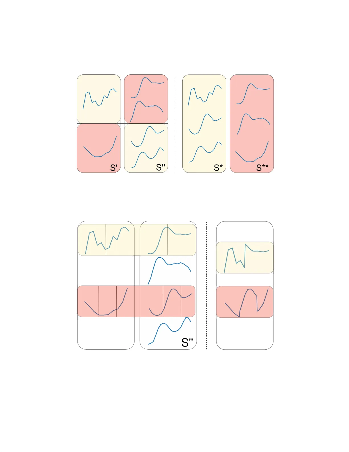
GENDIS: GENetic DIscovery of Shapelets Gilles V andewiele, Femke Ongenae, and Filip De T urck IDLab, Ghent University – imec, 9052 Ghent, B elgium { firstname } . { lastname } @ug ent.be Abstract. In the time series classification domain, shapelets are small time series that ar e discriminative for a cer tain class. It has been shown that classifiers are able to achieve state-of-the-art results on a p l ethora o f datasets by taking as input di s tances from the input time ser i es to different dis- criminative shapelets. Additionally , these shapelets can easily be visual- ized and thus pos sess an interpretable characteristic, making them very appealing in critical do mains, such as the health care domain, where lon- gitudinal d ata is ubiquitous. In this study , a new p ar adigm for shapelet discovery is propos ed, which is based upon evolutionary computation. The advantages of the proposed approach are that (i) it i s g r adient-free, which co ul d allow to es cape from local optima more easi ly and to find suited candidates more easily and supports non-differentiable objectives, (ii) no brute-force search i s required, which dr astically reduces the com- putational complexity by several orders of magnitude, (iii) the total amount of shapelets and length of each of these shapelets are evolved jointly with the shapelets themselves, alleviating the need to specif y this beforehand, (iv) e ntire sets are evaluated at once as oppose d to single shapelets, which results in smaller final se ts with less similar shapelets that result in similar predictive perfor mances, and ( v) di scovered shapelets do not need to be a subsequence of the input time seri es. W e present the results of ex p e ri- ments which validate the enumerated advantages. Keywords: genetic a lgorithms, time series classification, time serie s analysis, interpretable machine learning, da ta mining. 1 Introduction 1.1 Background Due to the uprise of the Internet-of-Things (IoT), mass adoption of sensors in all domains, including c r itical domains such as health care, ca n be noticed. These sensors produce d ata of a longitudinal form, i.e. time series. T ime series differ from classical tabula r data, since a temporal dependency is present where each value in the time series correlates with its neighboring values. One important task that emerges from this type of da ta is the cla ssification of time series in their entirety . A model able to solve such a task can be applied for a wide variety of 2 Gilles V andewiele, Femk e Ongenae, and F ilip De T urck applications, such as distinguishing betwee n normal brain activity and epilep- tic a ctivity (Chaovalitwongse et al., 200 6), determining different types of phys- ical activity (Liu et al., 20 1 5), or profiling electronic appliance usage in smart homes ( Li et al., 201 6). Often, the largest discriminative power can be found in smaller subsequences of these time serie s, ca lled shapelets. Sha pelets semanti- cally represent intelligence on how to discriminate between the different targets of a time series dataset ( Gra bocka et al., 20 14). W e can use a set of shapelets and the corresponding distances from each of these shapelets to ea ch of the input time series as features for a c la ssifier . It has been shown that such an approach outperforms a nearest neighbor search based on d ynamic time warping dis- tance on almost every dataset, which was deemed to be the state - of-the-art for a long time (Abanda et al., 2019). Moreover , shape lets possess an interpretable characteristic since they can easily be visualiz ed a nd be retrac e d back to the in- put signal, making them very interesting for decision support ap plications in critical domains, such as the medica l domain. In these critical domains, it is of vital importance that a corresponding explanation can be provided alongside a prediction, since a wrong decision can have a significant negative impact. 1.2 Relate d W ork Shapelet discovery was initially proposed by Y e and Keogh (2009). Unfortu- nately , the initial algorithm quickly becomes intractable, eve n for smaller da tasets, because of its la rge c omputational complexity ( O ( N 2 M 4 ) , with N the number of time series a nd M the length of the smallest time series in the da taset). This complexity wa s improved two years later , when Mueen et al. (20 11) proposed an extension to this algorithm, that make s use of caching for fa ster distance computation a nd a be tter upper bound for ca ndida te pruning. These improve- ments reduce the complexity to O ( N 2 M 3 ) , but have a la rger memory footprint. Rakthanmanon and Keogh (2013) proposed an approximative algorithm, called Fast S hapelets ( F S ), that finds a suboptimal shapelet in O ( N M 2 ) by first tra ns- forming the time series in the original set to Symbolic Aggregate ap p roXima- tion ( S A X ) representation s (Lin et al., 2003). A lthough no gua rantee can be ma d e that the discovered shapelet is the one that maximizes a pre-defined metric, they show they are able to achieve very similar classification performances, em- pirically on 32 d a tasets. All the aforementioned techniques search for a single shapelet that optimizes a cer tain metric, such as information gain. Often, one shapelet is not enough to a chieve good predictive performance s, especially f or multi-class classifica- tion problems. Therefore, the shape let discovery is applied in a recursive fa sh- ion in order to construct a decision tree. Lines et a l. (2012) p roposed Shape le t T ransform ( S T ), which performs only a single pa ss through the time series dataset a nd maintains a n ordered list of shapelet c andidates, ra nked by a met- ric, and then finally takes the top-k from this list in order to construct f eatures. While the algorithm only performs a single pa ss, the computational complexity still remains to be O ( N 2 M 4 ) , which makes the technique intractable for larger GENDIS: GENetic DIscovery of Shapelets 3 datasets. Extensions to this te chnique ha ve been proposed in the subsequent years which drastically improved the performance of the technique (Hills e t al., 2014; Bostrom and Bagnall, 201 7). Lines et al. (201 2) compared their technique to 36 other algorithms for time series classification on 85 datasets (Bagnall et al., 2017), which showed that their technique is one of the top-performing algo- rithms for time series classification and the be st- p e rforming shapelet extra ction technique in terms of predictive perf ormance. Grabocka et al. (2014) proposed a technique where shapelets are learned throug h gradient descent, in which the linear separa bility of the classes after transforma- tion to the distance space is optimized, called L earning T ime Series S ha pelets ( L T S ). The technique is competitive to S T , while not requiring a brute-force search, making it tracta ble for larger datasets. Unfortunately , L T S requir es the user to specify the number of shapelets and the length of ea ch of these shapelets, which can result in a rather time-intensive hyper-para meter tuning process in order to achieve a good predictive pe rformance. Three extensions of L T S which im- prove the computational runtime of the algorithm, have been proposed in the subsequent years. Unfortunately , in order to achieve these speedups, predic- tive performance had to b e sacrificed. A first extension is ca lled Sca lable Dis- covery ( S D ) (Grabocka et a l., 2 015). It is the fastest of the three e x tensions, im- proving the runtime two to three orders of magnitude, but at a cost of having a worse predictive performance than L T S on almost every tested dataset. Second, in 2 015, Ultra- Fa st Shapelets ( U F S ) (W istuba et al., 2015) wa s proposed. It is a better compromis e of runtime and predictive performance, as it is a n order of magnitude slower than S D , but sacrifices less of its predictive per formance. A final and most recent exte nsion is called Fused L A sso Generalized eigenvector method ( F L A G ) (Hou et a l., 2 016). It is the most notable of the three extensions as it has runtimes competitive to S D while being only slightly worse than L T S in terms of predictive performance. 1.3 Our Contribut i on In this pap e r , we introduce an evolutionary algorithm, G E N D I S , that discov- ers a set of shapelets from a collection of labeled time series. The aim of the proposed a lgorithm is to a chieve state - of-the-art p redictive perf ormances sim- ilar to the best-perf orming algorithm, S T , with a smaller number of shapelets, while having a low computational complexity similar to L T S . The goal of G E N D I S is to retain some of the positive properties from L T S such as its scalab le computational complexity , the fact that entire sets of shapelets are discovered as opposed to single shapelets and that it can discover shapelets outside the original dataset. W e de monstrate the a dded value of these two fi- nal properties through intuitive exp e riments in Subsections 3.2 and 3. 3 respec- tively . Moreover , G E N D I S has some benefits over L T S . First, genetic algorithms are gradient-free, allowing for any objective function a nd an easier escape from local optima. Second, the total amount of shapelets and the length of each of 4 Gilles V andewiele, Femk e Ongenae, and F ilip De T urck these shapelets do not need to be defined p r ior to the discovery , allevia ting the need to tune this, which could be computationally expensive a nd may require domain knowledge. Finally , we show by a thorough comparison, in Subsec- tion 3.5, that G E N D I S empirically outperforms L T S in terms of predictive per- formance. 2 Methodology In the f ollowing section we will first explain some general concepts from the time series analysis and shapelet discovery domain, on which we will then build further to elab orate our proposed algorithm, G E N D I S . 2.1 T ime serie s Matrix & Labe l V ector The input to a shapelet discovery algorithm is a collection of N time series. For ease of notation, we will assume that the time series are synchr onized a nd have a fixed length of M , resulting in a n input matrix T ∈ R N × M . It is important to note that G E N D I S could pe rfectly work with variable length time series as well. In that case, M would be e qual to the minimal time ser ies length in the collection. Since shapelet discovery is a supervised approach, we also require a label vector y of length N , with each element y i ∈ { 1 , . . . , C } a nd C the number of classes and y i corresponding to the label of the i -th time series in T . 2.2 Shapel e ts and Shap e let Se ts Shapelets are small time series which semantically represent intelligence on how to discriminate between the d ifferent targets of a time ser ies d ataset. In other words, they are very similar to subsequences from time series of ce rtain (groups of) c la sses, while be ing dissimilar to subsequences of time series of other classes. The output of a shapelet discovery algorithm is a collection of K shapelets, S = { s 1 , . . . , s K } , called a shapelet set. In G E N D I S , K and the length of ea c h shapelet does not need to be set beforehand and each shapelet can have a variable length, smaller than M . These K shapelets can then be used to extract features for the time series, a s we will expla in subsequently . 2.3 Distance Matrix Calcu lation Given an input matrix T and a shapelet set S , we can construct a p airwise distance matrix D ∈ R N × K : dist ( S , T ) = D The distance matrix, D , is constructed by calculating the distance be tween each ( t , s ) -pair , where t ∈ T i s an input time series and s ∈ S a shapelet from the candidate shapelet set. This matrix can then be f ed to a machine learning cla s- sifier . Often, K << M such that we effectively reduce the dimension of our GENDIS: GENetic DIscovery of Shapelets 5 data. In order to calculate the distance from a shapelet s in S to a time ser ie s t from T , we convolute the shapelet across the time series and take the minimum distance: dist ( s, t ) = min 1 ≤ i ≤ | t |−| s | d ( s, t [ i : i + | s | − 1]) with d ( . ) a distance metric, such a s the Euclidean distance, and t [ i : i + | s | − 1] a slice from t starting at index i and having the same length as s . 2.4 Shapel e t Set Discovery Obj ective Conceptually , the goal of a shapelet set extra ction tec hnique is to find a set of shapelets, S , that produces a distance matrix, D , that minimizes the loss f unc- tion, L , of the machine lea rning technique to which it is f ed, h ( . ) , given the ground truth, y . min S L ( h ( dist ( T , S )) , y ) It should be noted that the shapelet extra ction and classification phases a re completely decoupled, a s depicted in Figure 1. A set of shapelets ( S ) is first independently mined, which is then used to transform the time series into fea- tures that correspond to distances from ea ch of the time series to the shapelets in the set. These f e atures are then fed to a machine learning classifier . T raining timeseries T esting timeseries Shapelets T rain distances GENDIS T est distances Classi fi er fi t evaluat e fi t transform transform Fig. 1: A schematic overview of shapelet discovery . First, shapelets are indepen- dently extra cted using the training set. These shapelets are then used to trans- form the train and test set in features. A classifier can af terwards be fit on the training features a nd evaluated on the test features. 6 Gilles V andewiele, Femk e Ongenae, and F ilip De T urck 2.5 G E N D I S : GENe tic Discovery of Int erpretable S h apelet s In this paper , we propose a genetic algorithm that evolves a set of variable- length shapelets, S , in O ( N M 2 ) which produces a distance matrix D , based on a c ollection of time series T , that results in optimal predictive performance when provided to a machine le a rning classifier . The intuition behind the ap- proach is similar to L T S , which we mentioned in Section 1.2, but the adva ntage is that b oth the size of S , K , and the le ngth of ea c h shapelet s ∈ S are evolved jointly , alleviating the need to specify the number of shapelets a nd the length of each shapelet prior to the extra c tion. M oreover , the technique is gra dient-free, which allows for non-differentiable objectives a nd to escape local optima more easily . The building blocks of a genetic a lgorithm consist of at least a crossover , mu- tation and selection operator (Mitchell, 1998). Add itionally , we seed, or initial- ize, the algorithm with specific candidate s instead of completely random can- didates (Julstrom, 1994) and apply elitism (Shebl ´ e, 199 5) to make sure the fittest candidate set is never disca rded from the population or never experie nce s mu- tations that detriment its fitness. Each of these opera tions are elaborated upon in the following subsections. Initiali zation In order to seed the algorithm with initial candidate sets, we generate P candidate sets S ′ containing K shapelets, with K a ra ndom integer picked uniformly f rom [2 , W ] , W a hyper-par ameter of the algorithm, and P the population size. K is randomly chosen for each individual and the def ault value of W is set to be √ M . These two boundaries are chosen to be low in order to start with smaller candidate sets and grow them incrementally . This is beneficial f or both the size of the final shape let set as well as the runtime of each generation. For eac h candidate set we initialize, we randomly pick one of following two strategies with equal probability: Initiali zation 1: apply K - means on a set of random subser ie s of a fixed ra ndom length sampled from T . The K resulting centroids form a candidate set. Initiali zation 2: generate K candida tes of ra ndom lengths ( ∈ { 4 , . . . , max l en } ) by sampling them from T . The max l en is a hyper-parameter that limits the length of the discovered shapelets, in order to combat over fitting. While Initia lizati on 1 results in strong initial in- dividuals, Init i aliza t ion 2 is included in order to increase population diver sity and to decrease the time required to initialize the entire population. Fitness One of the most important components of a genetic algorithm, is its fitness function. In order to determine the fitness of a candida te set S ′ we first construct D ′ , which is the distance matrix obtained by ca lculating the distances between S ′ and T . The goal of our genetic algorithm is find a n S ′ which pro- duces a D ′ that results in the most optimal predictive perf ormance when pro- vided to a classifier . W e mea sure the p redictive per formance directly by means GENDIS: GENetic DIscovery of Shapelets 7 of an error function de fined on the predictions of a logistic regression model and the provided label vector y . When two candida te shapelet sets produce the same error , the set with the lowest complexity is d eemed to be the fittest. The complexity of a shapelet set is exp ressed as the sum of shapelet lengths ( P s ∈ S | s | ). The fitness ca lculation is the bottleneck of the algorithm. Calculating the dis- tance of a shapelet with length L to a time series of length M requires ( M − L + 1) × L pointwise comparisons. Thus, in the worst case, O ( M 2 ) operations need to be performed per time series, resulting in a computational complexity of O ( N M 2 ) . W e a pply these distance calculations to each individual representing a collection of shapelets f rom our population, in each generation. Therefore, the complexity of the entire a lgorithm is equal to O ( GP K N M 2 ) , with G the total number of genera tions, P the population size, and K the ( maximum) number of shapelets in the bag each individual of the population represents. Crossover W e define three different crosso ver operations, which take two can- didate shapelet sets, S ′ and S ′′ , as input and produce two new sets, S ∗ and S ∗∗ : Crossover 1: apply one- or two-point cro ssover on two shapelet sets (each with a probability of 5 0 %). In other words, we create two new shapelet sets that are composed of shapelets from both S ′ and S ′′ . An example of this opera- tion is provided in Figure 2. Crossover 2: iterate over e ach shapelet s in S ′ and apply one- or two-point crossover (aga in with a probability of 50% ) with another ra ndomly cho- sen shapelet from S ′′ to create S ∗ . Apply the same, vice versa, to obtain S ∗∗ . This differs from the first crossover opera tion as the one- or two-point crossover a re performed on individual shape lets as opposed to entire sets. An example of this operation can be see n in Figure 3 . Crossover 3: iterate over each shapelet s in S ′ and merge it with a nother ran- domly chosen shapelet from S ′′ . The merging of two shapelets ca n be done by calculating the mean (or barycenter) of the two time series. When two shapelets being merged have va r ying length, we merge the shorter shapelet with a random part of the longer shapelet. A schematic overview of this strategy , on shapelets having the same length, is depicted in Figure 4. It is possible that all or no techniques are a pplied on a pair of individuals. Each technique has a probability equal to the configur ed crossover probabil- ity ( p crossover ) of being app lied . Mutations The mutation operators a re a vital part of the genetic algorithm, as they ensure population diversity and allow to esca pe from local optima in the search spa ce. They take a ca ndidate set S ′ as input and produce a new , modified S ∗ . In our approach, we define three simple mutation operators: 8 Gilles V andewiele, Femk e Ongenae, and F ilip De T urck Fig. 2: A n example of a one-point crossover operation on two shapelet sets. Each original set is partitioned in two, and we take a partition from ea ch set in order to construct a new set. S' S* Fig. 3: An example of one- and two-poin t cros sover applied on individual shapelets. GENDIS: GENetic DIscovery of Shapelets 9 S* Fig. 4: An example of the shape le t merging crossover operation. Mutation 1: take a random s ∈ S ′ and randomly remove a variab le a mount of data points from the beginning or ending of the time series. Mutation 2: remove a random s ∈ S ′ . Mutation 3: create a new candidate using Init ializa tion 2 and add it to S ′ . Again, all techniques ca n be applied on a single individual, each having a p rob- ability equal to the configured mutation probability ( p mutation ). Select i on, El itism & Early S topping After e ach generation, a fixed number of candidate sets a re chosen based on their fitness for the next generation. M any different techniques exist to select these candidate sets. W e chose to a pply tour- nament selection with small tournament sizes. In this strategy , a number of candidate sets are sampled uniformly from the entire population to form a tour- nament. Afterwards, one c a ndidate set is sampled from the tournament, where the probability of being sampled is d e termined by its fitness. S maller tourna- ment sizes ensure better population diversity as the p robability of the fittest individual being included in the tournament decreases. Using this strategy , it is however possible that the fittest candida te set from the population is never chosen to compete in a tournament. Therefore, we a p p ly elitism and guar antee that the fittest candidate set is always transferred to the next generation’s popu- lation. Finally , since it can be hard to determine the ideal number of generations that a genetic algorithm should run, we implemented early stopping where the algorithm preemptively stops as soon as no candidate set with a better fitness has been found for a certain number of iterations ( patie nce ). 10 Gilles V andewiele, Femk e Ongenae, and F ilip De T urck List of all hyper-parame t ers W e now present an overview of a ll hyper-parameters included in G E N D I S , along with their corresponding explanation and d efault values. – Maximum shapelets per candida te ( W ) : the maximum number of shapelets in a newly genera ted individual during initialization ( default: √ M ). – Population size ( P ): the total number of candida tes that are eva luated and evolved in eve r y iter ation (default: 100 ). – Maximum number of genera tions ( G ): the max imum number of iter a tions the algorithm runs (def ault: 1 00 ). – Early stopping patience ( pati ence ): the algorithm preemptively stops evolv- ing when no bette r individual has b e en f ound for patie nce iterations ( de- fault: 10 ). – Mutation probability ( p mutation ): the probability that a mutation operator gets applied to a n individual in ea ch ite r ation (default: 0 . 1 ). – Crosso ver probability ( p crossover ): the probability that a crosso ver operator is applied on a pair of individuals in each iteration (def ault: 0 . 4 ). – Maximum shapelet length ( max l en ): the maximum length of the shapelets in each shapelet set (individual). (def ault: M ) . – The operations used during the initialization, c rossover a nd mutation phases are configurable a s well. (de fault: a ll mentioned operations). 3 Results In the following subsections, we will present the setup of different expe riments and the corresponding results in order to highlight the advanta ge s of G E N D I S . 3.1 Efficiency of genetic operators In this section, we a ssess the efficiency of the introduced genetic operators by evaluating the fitness in function of the number of generations using differ- ent sets of operators. It should be noted that our implementation easily allows to configure the number a nd type of operators used f or e a ch of the different steps in the genetic a lgorithm, allowing the user to tune these according to the dataset. Dataset s W e pick six datasets, with varying charac te ristics, to ev a luate the fit- ness of d ifferent configurations on. The chosen datase ts, and their correspond- ing properties a re summarize d in T able 1. Initiali zation ope rators W e first compare the fitness of GENDIS using three different sets of initialization oper ators: – Initializing the individuals with K-M eans (Initialization 1) – Randomly initializing the shapelet sets (Initialization 2) GENDIS: GENetic DIscovery of Shapelets 11 Dataset #Cls TS len #T rain #T es t ItalyPowerDemand 2 24 67 1029 SonyAIBORo bo tSurface2 2 65 27 953 FaceAll 14 131 560 1690 W ine 2 234 57 54 PhalangesOutlinesCorrect 2 80 1800 858 Herring 2 512 64 64 T able 1: The chosen data sets, having varying character istics, for the eva luation of the genetic operators’ efficiency . #Cls = number of classes, TS len = length of time series, #T rain = number of training time ser ies, #T rain = number of testing time series – Using all two initialization operations Each configuration was tested using a small population ( 25 individuals), in or- der to reduce the required c omputational time, for 7 5 generations, a s the im- pact of the initialization is highest in the e a rlier generations. All mutation a nd crossover operators were used. W e show the average fitness of all individu- als in the population in Figure 5. From these results, we can conclude that the two initializa tion operators are competitive to e a ch other , a s one operator will outperform the other on several datasets and vice versa on the others. Fig. 5: The fitness in function of the number of genera tions, for six data sets, using three different configurations of initialization operations. Crossover operat ors W e now compare the a verage fitness of a ll individuals in the population, in function of the number of generations, when configuring GENDIS to use f our different sets of crossover operators: 12 Gilles V andewiele, Femk e Ongenae, and F ilip De T urck – Using solely point crossovers on the shapelet sets (Crossover 1) – Using solely point crossovers on individual shapelets (Crossover 2 ) – Using solely merge crossovers ( Crossover 3) – Using all three crossover operations Each run had a population of 2 5 individuals and ran f or 2 00 generations. All mutation and initialization operators were used. As the average fitness is rather similar in the earlier generations, we truncate the first 5 0 measurements to bet- ter highlight the d ifferences. The results a re presented in Figure 6. As can be seen, it is aga in difficult to single out an opera tion that significantly outper- forms the others. Fig. 6: The fitness in function of the number of genera tions, for six data sets, using four different configurations of crossover opera tions. Mutation operat ors T he same ex periment was perf ormed to assess the effi- ciency of the mutation operators. Four different configurations were used: – Masking a random par t of a shapelet (Mutation 1 ) – Removing a random shapelet f rom the set (Mutation 2) – Adding a shapelet, ra ndomly sampled from the d ata, to the set (M utation 3) – Using all three mutation operations The ave rage fitness of the individuals, in function of the number of generations is depicted in Figure 7 . It is clea r that the ad d ition of shapelets (M utation 3) is the most significant operator . W ithout it, the fitness quickly converges to a sub- optimal value. The removal and masking of shapelets does not seem to increase the average fitness often, but are important operators in order to keep the the number of shapelets and the length of the shapelets small. GENDIS: GENetic DIscovery of Shapelets 13 Fig. 7: The fitness in function of the number of genera tions, for six data sets, using four different configurations of mutation operations. 3.2 Evaluati ng sets of ca ndidate s versus single cand idates A key factor of G E N D I S , is that it evaluates entire sets of shapelets ( a de pen- dency between the shapelets is introduced), as opposed to eva lua ting single candidates independently and taking a top-k. The disad vantage of the latter approach is that similar shapelets will achieve similar values given a certain metric. When entire sets are evaluated, we ca n both optimize a quality met- ric for candidate sets, as the size of each of these sets. This results in smaller sets with less similar shapelets. M oreover , intera c tions b e tween shapelets can be exp licitly taken into account. T o demonstrate these adva ntages, we compare G E N D I S to S T , which evaluates candidate shapelets individually , on an artifi- cial three-class dataset, depicted in Figure 8 . The constructed d ataset contains a large number of very similar time series of class 0, while ha v ing a smaller number of more dissimilar time series of class 1 a nd 2 . The distribution of time series across the three classes in both the train a nd test dataset is thus skewed, with the number of sa mples in cla ss 0 , 1 , 2 being equal to 25 , 5 , 5 respectively . This imba la nce causes the indepe nde nt approach to focus solely on extracting shapelets that c an discriminate cla ss 0 from the two others, since the informa- tion gain will be highest for these individual shapelets. Clear ly , this is not ideal as subsequences taken f rom time series of class 0 possess little to no discrimina- tive power f or the two other classes, as the distances to time series f rom these two classes will be nearly equal. W e extract two shapelets with both techniques, which allows us to visualize the different te st samples in a two-dimensional transformed distance space, a s shown in Figure 9. Each a xis of this space represents the distances to a certain shapelet. For the independent a pproach, we can clearly see that the distances of 14 Gilles V andewiele, Femk e Ongenae, and F ilip De T urck the samples for all three cla sses to both shap e lets are clustered near the origin of the space, making it very hard f or a cla ssifier to draw a separa tion boundary . On the other hand, a very clear separation can be seen for the sa mples of the three classes when using the shapelets discovered by G E N D I S , a dependent ap- proach. The low discriminative power of the indepent approach is confirmed by fitting a Logistic Regression model with tuned regulariza tion type and strength on the obtained distances. The classifier fitted on the distances extra cted by the independent approach is only a ble to achieve an accuracy of 0 . 82 86 ( 29 35 ) on the rather stra ight-forward dataset. The accuracy score of G E N D I S , a depe ndent approach, equals 1 . 0 . Fig. 8: The generated train a nd test set for the a rtificial classification problem. 3.3 Discovering shape lets outs i de the d ata Another a dvantage of G E N D I S , is that the discovery of shapelets is not lim- ited to be a subseries f rom T . Due to the nature of the evolutionary process, the discovered shapelets can have a distance greater than 0 to a ll time series in the data set. More formally: ∃ s ∈ S . ∀ t ∈ T . dist ( s, t ) > 0 . While this can be somewhat detrimental concerning interpretability , it can be necessary to ge t an excellent predictive performance. W e demonstrate this through a very simple, artificial example. Assume we hav e a two-class classification problem and are provided two time series pe r class, as illustrated in Figure 10a. The ex tracted shapelet, and the distances to each time series, by a brute force approach and a slightly modified v e rsion of G E N D I S ca n be found in Figure 10b. The modifi- cation we made to G E N D I S is that we specifically search for only one shapelet instead of an e ntire set of shap e lets. W e can see that the e x haustive search ap- proach is not able to find a subseries in a ny of these four time series that sepa - rates both classes while the shapelet extra cted by G E N D I S ensures p e rfect sep- aration. It is important to note here that discovering shapelets outside the data sacrifices interpretability for a n increase in predictive performance of the shapelets. As GENDIS: GENetic DIscovery of Shapelets 15 Fig. 9: The samples of the test set are represented by mar kers (circles for G E N D I S ) a nd crosses for S T ) while the axes correspond to the distance to a shapelet. the oper ators that are used d uring the genetic algorithm are completely con- figurable for G E N D I S , one can use only the first crossover operation (one- or two-point crossover on shapelet sets) to ensure a ll shapelets come from within the data. 3.4 Stabil i ty In order to eva luate the stability of our algorithm, we compare the extr acted shapelets of two different runs on the ItalyPowerDemand data set. W e set the algorithm to e volve a large population (1 00 individuals) for a large number of generations (500) in order to ensure convergence. Moreover , we limit the max - imum number of ex tr acted shapelets to 10, in order to kee p the visualization clear . W e then calculated the similarity of the d iscovered shapelets between the two runs, using Dynamic T ime W a rping (Ber ndt a nd Clifford , 199 4). A heatmap of the distances is d epicted in Figure 11. While the discovered shapelets are not exactly the same, we can often find pa ir s that c ontain the same semantic intelli- gence, such as a sa w pattern or straight lines. 16 Gilles V andewiele, Femk e Ongenae, and F ilip De T urck (a) (b) Fig. 10: A two-class problem with two time series per class and the extr a cted shapelets with corresponding d istances on a n ordered line by a brute-f orce ap- proach versus G E N D I S . The crosses on the ordered line correspond to distances of the shapele t to the time series f rom Class 1 while the circles on the ordered line correspond to distances to Class 0 (the more to the right, the higher the distance). 3.5 Comparing G E N D I S to F S , S T and L T S In this section, we compare our algorithm G E N D I S to the results from (Bagnall et a l., 2017), which are hosted online 1 . In that study , 31 different algorithms, includ- ing three shapelet discovery techniques, have been compared on 85 da tasets. The 85 da tasets stem from different da ta sources and different domains, includ- ing electrocardiogram data from the medical domain and sensor data from the IoT domain. The three included shapelet techniques are S hapelet T ransform ( S T ) ( L ines et al., 2 012), Learning T ime Series Shap e lets ( L T S ) ( Gra bocka et al., 2014), and Fast Shapelets ( F S ) (Rakthanmanon and Keogh, 201 3). A d iscussion of all three techniques can be f ound in Section 1.2. For 8 4 of the 85 da tasets, we conducted twelve measurements by concatenat- ing the provided training and testing data and re-par titioning in a stratified manner , as done in the original study . Only the ‘Phoneme’ dataset could not be included d ue to problems downloading the data while exe cuting this e x- periment. On every dataset, we used the same hyper-parameter configuration for G E N D I S : a population size of 100, a maximum of 1 00 iterations, ear ly stop- ping a f ter 10 iterations a nd crossover & mutation probabilities of 0 . 4 and 0 . 1 respectively . T he only parameter that was tuned for every da taset separ ately was a ma ximum length for each shapelet, to combat overfitting. T o tune this, we picked the length l ∈ [ M 4 , M 2 , 3 M 4 , M ] tha t resulted in the best logarithmic (or entropy) loss using 3-fold cross validation on the tra ining set. The distance matrix obtained throu gh the extracted shapelets of G E N D I S was then fed to 1 www.timeserie sclassificatio n.com GENDIS: GENetic DIscovery of Shapelets 17 Fig. 11: A pa irwise d ista nce matrix, constructed using Dynamic T ime W arping, between discovered shapelet sets of two different runs on the ItalyPowerDe- mand data set. a heterogeneous ensemble consistin g of a rotation forest, random forest, sup- port vector machine with linear kernel, support vector with quadratic ke r nel and a k-nearest neighbor classifier (Large et a l. ( 2 017)). This ensemble matches the one used by the best-perf orming algorithm, S T , closely . This is in contrast with F S which produces a decision tree and L T S which le a rns a separa ting hy- perplane (similar to logistic regression) jointly with the shapelets. This setup is also d epicted schematica lly in Figure 1 2. T rivially , the ensemble will em- pirically outperform e ach of the individual classifiers ( ? ) , but it does take a longer time to fit and somewhat takes the focus away f rom the quality of the extracted shape lets. Nevertheless, it is necessar y to use an ensemble in order to allow for a f air comparison with S T , as tha t wa s used by Ba gna ll et al. (20 17) to generate their results. T o give more insights into the quality of the e xtracted shapelets, we a lso report the accuracies using a Logistic Regression classifier . W e tuned the type of regularization (Ridge vs Lasso) and the regularization strength ( C ∈ { 0 . 001 , 0 . 01 , 0 . 1 , 1 . 0 , 10 . 0 , 100 . 0 , 1000 . 0 } ) using the tra ining set. W e recommend future research to compare their results to those obtained with 18 Gilles V andewiele, Femk e Ongenae, and F ilip De T urck Logistic Regression classifier . test train + data test' train' Strati fi ed split GENDIS K-Nearest Neighbors Linear SVM Quadratic SVM Rotation Forest Random Forest W eighted ensemble T une length Fig. 12: The evalua tion setup used to compare G E N D I S to other shapelet tech- niques. T rain and test d ata are first concatenated and then re-distributed to form new train and te st sets with similar distributions to the ones prior to the con- catenation. T he newly created train set is then used to tune the optimal maximal length of the shapelets in cross-validation and used to extra ct shape lets and to train the e nsemble of classifiers. Finally , the test set is used to e v a luate the ex- tracted shapelets and fitted ensemble. The mean a ccuracy over the twelve mea surements of G E N D I S in comparison to the mean of the hundred original measurements of the three other algorithms, retrieved from the online repository , c an be f ound in T able 2 and 3. While a smaller number of measurements is conducted within this study , it should be noted that the measurements f rom B agnall et al. (2 017) took over 6 months to generate. Moreover , accura cy is often not the most ideal metric to measure the predictive performance with. A lthough it is one of the most intuitive metrics, it has several disa d vantages such as skewness when data is imbalanced. Never- theless, the a ccuracy metric is the only one allowing for comparison to related work, as that metric was used in those studies. Moreover , the used datasets are merely benchmark datasets and the goal is solely to compare the quality of the shapelets ex tr acted by G E N D I S to those of S T . W e recommend to use different performance metrics, which should be ta ilored to the spec ific use case. An ex- ample is using the area under the receiver operating chara cteristic curve (A UC) in combination with precision and recall for medical data sets. For each data set, we also perform a n unpaired student t-test with a cutoff value of 0 . 0 5 to detect statistically significant differences. When the perf ormance of an algorithm for a c ertain da taset is statistically better than all others, it is in- dicated in bold. From these results, we ca n conclude that F S is inferior to the three other techniques while S T most often a chieves the best performance, but at a very high computational complexity . GENDIS: GENetic DIscovery of Shapelets 19 The a v e rage number of shapelets extra c te d by G E N D I S is reported in the final column. The number of shape lets extra cted by S T in the original study equals 10 ∗ N . Thus, the total number of shapelets used to transform the original time series to distances is at least an order of magnitude less when using G E N D I S . In order to compare the algorithms across a ll data sets, a Friedman ranking test (Friedman (193 7)), was applied with a Holm post-hoc correction (Holm (1979); Benavoli et al. (2016)). W e present the average rank of ea ch algorithm using a critical difference diagra m, with cliques formed using the results of the Friedman test with a Holm post-hoc c orrection at a significance cutoff level of 0 . 1 in Figure 13. The higher the cutoff level, the less p robable it is to form cliques. For G E N D I S , b oth the results obtained with the ensemble and with the logistic regression classifier a re used. From this, we can c onclude that there is no statistical difference b e tween S T and G E N D I S while both are statistically bet- ter than F S and L T S . Fig. 13: A critical difference diagra m of the four eva luated shapelet discovery algorithms. For ea ch te chnique, the a v e rage ra nk is calculated . Then cliques (bold black lines) are formed if the p -value of the Holm post-hoc test is lower than 0 . 1 . 4 Conclusion In this study , an innovative technique, called G E N D I S , was proposed to ex tr act a collection of smaller subsequences, i.e. shapelets, f rom a time series da taset that are very informative in classifying e ach of the time series into categories. G E N D I S searches for this set of shapelets thro ugh evolutionary computation, a para digm mostly unexplored within the domain of time series cla ssification, which offers seve ral benefits: – evolutionary algorithms are gr a dient-free, allowing for an ea sy c onfigura- tion of the optimization objective, which does not need to be differentiable 20 Gilles V andewiele, Femk e Ongenae, and F ilip De T urck – only the max imum length of all shapelets has to be tuned, as opposed to the number of shapelets a nd a length of each shapelet, due to the fa c t that G E N D I S e valuates entire sets of shapelets – easy control over the runtime of the algorithm – the possibility of discovering shapelets that not need to be a subsequence of the input time series Moreover , the proposed technique has a c omputational complexity that is mul- tiple orders of magnitude smaller ( O ( GP K N M 2 ) vs O ( N 2 M 4 ) ) than current state-of-the-art, S T , while outperforming it in terms of predictive pe rformance, with much smaller shapelet sets. W e demonstrate these benefits thr ough intuitive ex p e riments where it was shown that techniques that ev aluate single ca ndid a tes can pe rform subpar on imbal- anced data sets and how sometimes the necessity ar ises to ex tract shapelets that are no subsequences of input time series to achieve good separa tion. In a ddi- tion, we compare the efficiency of the different ge netic operators on six differ- ent datasets a nd assess the algorithm’s stability by comparing the output of two different runs on the same da taset. Moreover , we conducted a n extensive com- parison on a large amount of datasets to show that G E N D I S is competitive to the current state - of-the-art while having a much lower computational complexity . 5 Reproducibility & code availability An implementation of G E N D I S in Python 3 is available on GitHub 2 . M oreover , code in order to perf orm the e xperiments to reproduce the results is included. 6 Acknowledgements G. V andewiele is funded by a PhD SB fellow scholarship of Fonds W etenschap- pelijk Onderzoek (FWO) (1S31 417N). F . Ongenae is f unded by a B ijzonder On- derzoeksFonds (BOF) grant from Ghent University . 2 https://githu b.com/IBCNServ ices/GENDIS GENDIS: GENetic DIscovery of Shapelets 21 Dataset #Cls TS len #T rain #T est GENDIS ST L TS FS #Shaps Ens LR Adiac 37 176 390 391 66.2 69.8 76.8 42.9 55.5 39 Arr owHead 3 251 36 175 79.4 82.0 85.1 84.1 67.5 39 Beef 5 470 30 30 51.5 58.8 73.6 69.8 50.2 41 BeetleFly 2 512 20 20 90.6 87.5 87.5 86.2 79.6 42 Bird Chicken 2 512 20 20 90.0 90.5 92.7 86.4 86.2 45 CBF 3 128 30 900 99.1 97.6 98.6 97.7 92.4 43 Car 4 577 60 60 82.5 83.0 90.2 85.6 73.6 48 ChlorineConcentration 3 166 467 3840 60.9 57.5 68.2 58.6 56.6 30 CinCECGT o rso 4 1639 40 1380 92.1 91.5 91.8 85.5 74.1 57 Coffee 2 286 28 28 98.9 98.6 99.5 99.5 91.7 44 Computers 2 720 250 250 75.4 72.7 78.5 65.4 50.0 38 CricketX 12 300 390 390 73.1 66.6 77.7 74.4 47.9 41 CricketY 12 300 390 390 69.8 64.3 76.2 72.6 50.9 41 CricketZ 12 300 390 390 72.6 65.9 79.8 75.4 46.6 40 DiatomSizeReduction 4 345 16 306 97.4 96.5 91.1 92.7 87.3 45 DistalPhalanxOutlineAgeGroup 3 80 400 139 84.4 83.2 81.9 81.0 74.5 32 DistalPhalanxOutlineCorrect 2 80 600 276 82.4 81.5 82.9 82.2 78.0 32 DistalPhalanxTW 6 80 400 139 76.7 76.0 69.0 65.9 62.3 33 ECG200 2 96 100 100 86.3 86.5 84.0 87.1 80.6 30 ECG5000 5 140 500 4500 94.0 93.8 94.3 94.0 92.2 34 ECGFiveDays 2 136 23 861 99.9 100.0 95. 5 98.5 98.6 33 Earthquakes 2 512 322 139 78.4 73.7 73.7 74.2 74.7 44 ElectricDevic es 7 96 8926 7711 83.7 77.6 89.5 70.9 26.2 31 FaceAll 14 131 560 1690 94.5 92.6 96.8 92.6 77.2 38 FaceFour 4 350 24 88 93.2 94.1 79.4 95.7 86.9 41 FacesUCR 14 131 200 2050 90.1 89.0 90.9 93.9 70.1 39 FiftyW ord s 50 270 450 455 72.9 71.8 71.3 69.4 51.2 39 Fish 7 463 175 175 87.0 90.5 97.4 94.0 74.2 50 FordA 2 500 3601 1320 90.8 90.7 96.5 89.5 78.5 37 FordB 2 500 3636 810 89.5 89.8 91.5 89.0 78.3 38 GunPoint 2 150 50 150 96.9 95.7 99.9 98.3 93.0 39 Ham 2 431 109 105 72.9 77.2 80.8 83.2 67.7 37 HandOutlines 2 2709 1000 370 89.7 91.0 92.4 83.7 84.1 41 Haptics 5 1092 155 308 45.2 43.9 51.2 47.8 35.6 55 Herring 2 512 64 64 59.6 61.8 65.3 62.8 55.8 42 InlineSkate 7 1882 100 550 43.8 39.3 39.3 29.9 25.7 58 InsectWingbeatSound 11 256 220 1980 57.3 57.5 61.7 55.0 48.8 36 ItalyPowerDemand 2 24 67 1029 95.6 96.0 95.3 95.2 90.9 31 LargeKitchenA ppliances 3 720 375 375 91.0 90.4 93.3 76.5 41.9 33 Lightning2 2 637 60 61 80.9 79.1 65.9 75.9 48.0 39 Lightning7 7 319 70 73 78.2 76.3 72.4 76.5 10.1 39 Mallat 8 1024 55 2345 98.2 97.3 97.2 95.1 89.3 58 T able 2: A comparison between G E N D I S a nd three other shapelet techniques on 85 da tasets. For each data set, we report the total number of classes, the length of the time series, the number of time series in the tra in and test set, the a ccu- racy score on the test set achieved by G E N D I S (using both an ensemble (E ns) and logistic regression (LR)), S T , L T S & F S , and finally the ave r age number of shapelets extrac ted b y G E N D I S . When a technique is statistically significant better than the others, according to a stude nt t-test with a cutoff of 0 . 0 5 , it is marked as bold. 22 Gilles V andewiele, Femk e Ongenae, and F ilip De T urck Dataset #Cls TS len #T rain #T es t GENDIS ST L T S FS #Shaps Ens LR Meat 3 448 60 60 98.7 98.8 96.6 81.4 92. 4 48 MedicalImages 10 99 381 760 72.4 68.6 69.1 70.4 60.9 37 MiddlePhalanxOutlineAgeGr oup 3 80 400 154 74.4 73.2 69.4 67.9 61.3 30 MiddlePhalanxOutlineCorr ect 2 80 600 291 80.7 79.6 81.5 82.2 71.6 30 MiddlePhalanxTW 6 80 399 154 62.2 63.1 57.9 54.0 51.9 37 MoteStrain 2 84 20 1252 86.3 86.6 88.2 87.6 79.3 36 NonInvasiveFatalECGThorax1 42 750 1800 1965 84.7 89.4 94.7 60.0 71.0 41 NonInvasiveFatalECGThorax2 42 750 1800 1965 87.1 92.3 95.4 73.9 75.8 37 OSULeaf 6 427 200 242 76.2 75.8 93.4 77.1 67.9 45 OliveOil 4 570 30 30 86.1 88.8 88.1 17.2 76.5 53 PhalangesOutlinesCorrect 2 80 1800 858 80.8 78.7 79.4 78.3 73.0 30 Plane 7 144 105 105 99.2 99.3 100.0 99.5 97.0 34 ProximalPhalanxOutlineAgeGr oup 3 80 400 205 84.1 83.9 84.1 83.2 79.7 32 ProximalPhalanxOutlineCorr ect 2 80 600 291 86.2 85.7 88.1 79.3 79.7 30 ProximalPhalanxTW 6 80 400 205 81.7 80.2 80.3 79.4 71.6 31 RefrigerationDevices 3 720 375 375 68.6 62.4 76.1 64.2 57.4 34 ScreenT ype 3 720 375 375 52.8 52.8 67.6 44.5 36.5 37 ShapeletSim 2 500 20 180 100.0 100. 0 93.4 93.3 100. 0 34 ShapesAll 60 512 600 600 79.6 79.3 85.4 76.0 59.8 44 SmallKitchenAppliances 3 720 375 375 74.3 74.2 80.2 66.3 33.3 37 SonyAIBORobotSurface1 2 70 20 601 96.0 95.6 88.8 90.6 91.8 34 SonyAIBORobotSurface2 2 65 27 953 88.6 87.0 92.4 90.0 84.9 34 StarLightCurves 3 1024 1000 8236 95.9 95.3 97.7 88.8 90.8 30 Strawberry 2 235 613 370 95.2 95.1 96.8 92.5 91.7 34 SwedishLeaf 15 128 500 625 88.7 87.7 93.9 89.9 75.8 37 Symbols 6 398 25 995 93.4 92.5 86.2 91.9 90.8 43 SyntheticControl 6 60 300 300 98.8 98.7 98.7 99.5 92.0 39 T oeSegm entation1 2 277 40 228 92.0 90.7 95.4 93.4 90.4 40 T oeSegm entation2 2 343 36 130 93.1 90.6 94.7 94.3 87.3 36 T race 4 275 100 100 100.0 99. 9 100.0 99.6 99.8 25 T woLeadECG 2 82 23 1139 95.8 96.6 98.4 99.4 92.0 36 T woPat terns 4 128 1000 40 00 95.8 93.1 95.2 99.4 69.6 33 UW aveGe stureLibraryAl l 8 945 896 3582 94.9 94.8 94.2 68.0 76.6 44 UW aveGe stureLibraryX 8 315 896 3582 80.2 77.9 80.6 80.4 69.4 42 UW aveGe stureLibraryY 8 315 896 3582 71.5 69.5 73.7 71.8 59.1 40 UW aveGe stureLibraryZ 8 315 896 3582 74.4 72.2 74.7 73.7 63.8 42 W afer 2 152 1000 6164 99.4 99.3 100.0 99.6 98.1 24 Wine 2 234 57 54 86.5 86.4 92.6 52.4 79.4 39 W or dSynonyms 25 270 267 638 68.4 62.8 58.2 58.1 46.1 42 W orms 5 900 181 77 65.6 59.9 71.9 64.2 62.2 47 W ormsT woClass 2 900 181 77 74.1 69.1 77.9 73.6 70.6 50 Y o ga 2 426 300 3000 83.3 80.2 82.3 83.3 72.1 40 T able 3: A comparison between G E N D I S a nd three other shapelet techniques on 85 da tasets. For each data set, we report the total number of classes, the length of the time series, the number of time series in the tra in and test set, the a ccu- racy score on the test set achieved by G E N D I S (using both an ensemble (E ns) and logistic regression (LR)), S T , L T S & F S , and finally the ave r age number of shapelets extrac ted b y G E N D I S . When a technique is statistically significant better than the others, according to a stude nt t-test with a cutoff of 0 . 0 5 , it is marked as bold. Bibliography Abanda, A., Mori, U., and Lozano, J. A. (2019). A review o n distance based time ser ies classification. Data Min ing and Knowledge Discovery , 33(2):378–412 . Bagnall, A., Li nes , J., Bos trom, A., Large, J., and Keogh, E. (2017). The great time serie s classification bake off: a review and exp e rimental evaluation of recent alg orithmic advances. Data Minin g an d Knowledge Discovery , 31(3):606–6 60. Benavoli, A., Corani, G., and Mangili, F . (2016). Should we really use post-hoc tests based on mean-ranks? The Journal of Machine Learnin g R esearch , 17(1):152–161. Berndt, D. J. and Clifford, J. (1994). Using dynamic time warping to find patterns in time series. In KDD workshop , volume 10, pages 359–370. Seattle, W A. Bostrom, A. and Bagnall, A. (2017). Bina ry shapelet transform for multiclass time se- ries classification. In T ransactions on Large-Scale Data-and Knowledge-Centered Systems XXXII , pages 24–46 . Springer . Chaovalitwongse, W . A., Prokopyev , O. A., and Pardalos, P . M. (2006 ). Electroencephalo- gram (eeg) time series classification: Applications in epi l epsy . Annals of Operations Research , 148(1):227 –250. Friedman, M. ( 1937). The use of ranks to avoid the assumption of normality im p l icit in the analysis of variance. Journal of the american statistical association , 32(200):675–701. Grabocka, J., Schilling, N., Wistub a, M., and Schmidt-Thieme, L. (2014). Lear ning time- series shapelets. In Proceedings of the 20th ACM SIGK DD in ternational conference on Knowledge discovery an d data min ing , pages 392–401. ACM. Grabocka, J. , W istuba, M ., and Schmidt-Thieme, L. (2015). Scalable dis covery of time- series shapelets. arXiv preprint arXiv:1503.03 238 . Hills, J. , L ines, J., Baranauskas, E., Mapp, J., and Bagnall, A. (2014). Classification of time series by shapelet transformation. Data Min ing and Kn owledge Discovery , 28(4):851– 881. Holm, S. (1979). A simple sequentially rejective multipl e test p roced ure. Scandinavian journal of statisti cs , pages 65–70 . Hou, L. , Kwok, J. T ., and Zurada, J . M. (2016). Efficient learning of timeseries shapelets. In Thirtieth AAAI Conference on Arti ficial Intelligence . Julstrom, B . A. (1994). Seed ing the population: improved pe rformance in a genetic algo- rithm for the rectilinear s teiner problem. In Proceed ings of the 1994 ACM symposium on Applied computing , pages 222–226. ACM . Large, J., Li nes, J., and Bagnall, A. (2017). T he heterogeneous ensembles of standard classification algorithms (hesca): the whole is greater than the sum of its parts. arXiv preprint arXiv:1710.0922 0 . Li, D., B issyand ´ e , T . F . , Kubler , S., Klein, J., and Le T raon, Y . (2016). Profiling household appliance electricity usage with n-gram language model ing. In Indu st ri al T echnology (ICIT), 2016 IEEE International Conf erence on , pages 604–609. IEE E. Lin, J., Keog h, E., Lonardi, S., and Chiu, B. (2003). A symbolic representation of time series, with implications f o r streaming algorithms. In Proceedings of the 8th ACM SIG- MOD workshop on Research issues in data mining and kn owl edge discovery , pages 2–11. ACM. Lines, J., Davis, L. M ., Hills, J., and Bagnall, A. (2012). A shapelet transform for time series classification. In Proceedings of the 18th ACM SIGKDD international conference on Knowledge discovery an d data min ing , pages 289–297. ACM. 24 Gilles V andewiele, Femk e Ongenae, and F ilip De T urck Liu, L., Peng, Y ., Liu, M., and Huang, Z. (2015). Sensor-based human activity recogni- tion system with a mul til ayered model usi ng time ser ies shapelets. Knowledge-Based Systems , 90:138–152. Mitchell, M. (1998). An introduction to genetic algorithms . M IT press. Mueen, A., Keogh, E., and Y oung, N. (2011). Logi cal-s hapelets: an expressive p r imitive for time series classification. In Proceedings of the 17th ACM S I GKDD international conference on Knowledge discovery and data mining , pages 1154–1162. ACM. Rakthanman on, T . and Keogh, E. (2013). Fast shapelets: A scalable algorithm for dis cov- ering time serie s shapelets. In proceedings of the 2013 SIAM Intern ational Conf erence on Data Min i ng , pages 668–676. SIAM. Shebl ´ e, Gerald B Gand Brittig, K. ( 1995). Refined genetic alg orithm-economic dispatch example. IEEE T ransactions on Power Systems , 10(1):117–1 24. W i stuba, M., Grabocka, J. , and Schmidt-Thieme, L. (2015). Ultra-fast shapelets for time series classification. arXiv prep rint arXiv:1503.05018 . Y e, L. and Keo gh, E. (2009). T i me seri es shapelets: a new primitive f or data mining. In Proceedings of the 15th ACM SIGK DD international conference on Knowledge discovery and data mining , pages 947–956. ACM .