Sparse Pursuit and Dictionary Learning for Blind Source Separation in Polyphonic Music Recordings

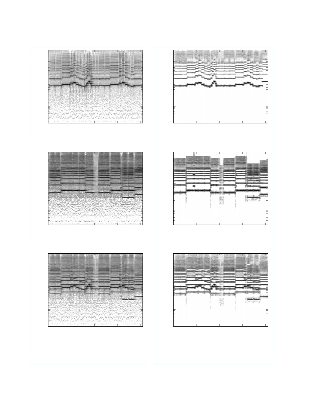
Schulze and King RESEARCH Spa rse Pursuit and Dictiona ry Lea rning fo r Blind Source Sepa ration in P olyphonic Music Reco rdings Sö ren Schulze 1 * and Emily J. King 2 Abstract W e p rop ose an algo rithm fo r the blind separation of single-channel audio signals. It is based on a parametric mo del that de scribes the sp ectral properties of the sounds of musical instruments indep endently of pitch. We develop a novel spa rse pursuit algo rithm that can match the discrete frequency sp ectra from the recorded signal with the continuous sp ectra delivered by the mo del. We ﬁrst use this algorithm to convert an STFT sp ectrogram from the recording into a novel form of log-frequency sp ectrogram whose resolution exceeds that of the mel sp ectrogram. W e then make use of the pitch-invariant properties of that representation in order to identify the sounds of the instruments via the same sparse pursuit metho d. As the mo del parameters which characterize the musical instruments are not known b efo rehand, we train a dictionary that contains them, using a mo diﬁed version of Adam. Applying the algorithm on va rious audio samples, we ﬁnd that it is capable of p ro ducing high-qualit y sepa ration results when the mo del assumptions are satisﬁed and the instruments are clearly distinguishable, but combinations of instruments with similar sp ectral characteristics p ose a conceptual diﬃculty . While a key feature of the mo del is that it explicitly mo dels inharmonicit y , its p resence can also still imp ede p erfo rmance of the spa rse pursuit algo rithm. In general, due to its pitch-invariance, our metho d is esp ecially suitable fo r dealing with sp ectra from acoustic instruments, requiring only a minimal numb er of hyp erpa rameters to b e preset. Additionally , we demonstrate that the dictionary that is constructed for one recording can b e applied to a diﬀerent recording with similar instruments without additional training. Keyw o rds: Blind source separation; unsup ervised learning; dictionary learning; pitch-invariance; pattern matching; sparsit y; sto chastic optimization; Adam; orthogonal matching pursuit 1 Intro duction 1.1 Problem Deﬁnition and Approach Sour c e sep ar ation concerns the recov ery of signals X 1 , . . . , X c from a mixture X = X 1 + . . . + X c . W e sp eak of blind sep ar ation when no sp eciﬁc prior information to characterize the sources of the signals is provided, esp ecially not in the form of labeled training data. Ho wev er, we do make structur al assumptions about the signals; in our case, we assume that they follow the typical characterics of tones from wind and string instrumen ts. In order to exploit this structure, it is helpful to regard a time-frequency representation ( sp e ctr o gr am ), which sub divides the problem into smaller time frames and highligh ts the frequency characteristics of the signal. One simple sp ectrogram is obtained via the mo dulus of the short-time F ourier transform (STFT) (cf. [ 1 ]). * Correspondence: sschulze@uni-bremen.de 1 AG Computational Data Analysis, Facult y 3, Universit y of Bremen, Bibliothekstr. 5, 28359 Bremen, Germany Full list of autho r information is available at the end of the article Ho wev er, in the STFT sp ectrogram, diﬀeren t pitch of the instrument tones manifests in linear scaling of the distances b et ween the p eaks on the frequency axis, whic h makes it computationally hard to iden tify the tones in the sp ectrum. Th us, we apply a nov el sp arse pursuit algorithm that represen ts the time frames of the STFT sp ectrogram via a limited n um b er of p eaks, under the assumption that they originate from sinusoidal signals in the recording. W e then place these identiﬁed p eaks in a new sp ec- trogram that has a logarithmic frequency axis and is therefore pitch-invariant (cf. Section 3 ). On this, we apply a dictionary le arning algorithm, where the dic- tionary con tains the learned relative amplitudes of the harmonics for eac h instrument. In an alternating lo op, w e identify the sounds of the instruments by now ap- plying the sparse pursuit algorithm on time frames of the log-frequency sp ectrogram using the current v alue of the dictionary and then up date the dictionary based on that identiﬁcation. Both the problem of ﬁnding the p eaks in the STFT sp ectrogram and the problem of This is the autho rs’ manuscript (p ost p eer-review). In o rder to access the published a rticle, please visit: https://doi.org/10.1186/s13636- 020- 00190- 4 Schulze and King Page 2 of 25 Time-domain signal STFT Spectrogram Sparse Pursuit Log-frequency spectrogram Sparse pursuit Iterate Separated signals Griﬃn & Lim Spectral masking Separated spectrograms Sparse pursuit Dictionary Adam Figure 1 Data ﬂow diagram for the proposed separation method. The sparse pursuit algo rithm is used both for converting the STFT spectrogram into a log-frequency sp ectrogram and fo r identifying the instrument sounds in the log-frequency sp ectrogram. ﬁnding the patterns representing the instrumen t sounds are generally underdetermined (cf. Section 1.3 ), so spar- sit y pla ys a crucial role in their regularization. After training has ﬁnished, we apply the sparse pur- suit algorithm on the entire log-frequency sp ectrogram in order to obtain the separated sp ectrograms, and af- ter masking with the original mixture sp ectrogram, we emplo y the algorithm by Griﬃn and Lim [ 2 ] in order to con v ert them back into time-domain signals, using the phase of the original sp ectrogram as the initial v alue. The ov erall pro cedure is display ed in Figure 1 . The nov elt y of our approach lies in the combina- tion of pitc h-in v ariant representations with a sparse pursuit algorithm during training: Provided that the c haracteristics of the sounds of the instrumen ts are suﬃcien tly stable, the relative amplitudes of the har- monics sav ed in the dictionary represent the sounds of the instruments at any arbitrary pitch, without mak- ing assumptions ab out their tuning or range. At the same time, the use of a log-frequency axis enables us to match the sp ectrogram with the mo deled patterns of these sounds in an eﬃcien t manner, and due to a non-linear optimization step, the parameters are lo- cally optimal on a contin uous scale. As the outcome of the training is sometimes sensitive with resp ect to the initial dictionary , w e t ypically use the metho d in an ensem ble setting. Apart from the sparsity condition, there is no need to hand-tune any hyperparameters for a sp eciﬁc rec or ding. The sparse pursuit algorithm that w e prop ose is designed to m a tch a generic sampled sp ectrum with shifted non-negativ e contin uous patterns. While it was dev elop ed with audio frequency spectra in mind, it ma y b e used in other signal pro cessing applications as w ell. 1.2 Related Wo rk During the past years, audio source separation has b ecome a very wide ﬁeld, now incorp orating a num b er of fundamentally diﬀerent applications and approaches. A thorough o v erview can be found in bo oks on the sub ject that ha v e recen tly app eared [ 3 , 4 , 5 ]. The ﬁrst instance of learning the harmonic structure of m usical instruments via non-negative matrix factor- ization (NMF) [ 6 ] on sp ectrograms was by Smaragdis and Bro wn [ 7 ] for the purp ose of polyphonic music transcription. This approach was then applied to audio source separation by W ang and Plumbley [ 8 ]. The algo- rithm learns a dictionary where each atom represents one instrument at a sp eciﬁc pitch. By estimating the tones of the instruments at sp eciﬁc p oin ts in time, it is thereb y p ossible to reconstruct the contributions of the individual instruments. An ov erview of single-channel NMF-based metho ds can b e found in [ 9 ]. In many cases, a single m usical instrumen t can gen- erate diﬀerent sounds which are p erceptually similar and only v ary in the pitch of the tones. Using the c onstant-Q tr ansform (CQT) [ 10 ] as a log-frequency sp ectrogram, Fitzgerald et al. [ 11 ] use non-negative tensor factorization to generate a dictionary con taining the frequency sp ectra of diﬀerent instruments, which can b e shifted on a ﬁxed grid of semitones in order to apply them to diﬀerent notes. This approach was later reﬁned by Jaiswal et al. [ 12 , 13 , 14 ]. The adv an tage of this representation is that it can b e applied to a large v ariety of musical instruments, as long as pitc h-in v ariance is fulﬁlled. The drawbac k is that it requires the instrumen ts to b e tuned precisely to a known equal-temp eramen t scale, which mak es it impractical for real-world recordings with acoustic instrumen ts. Alternativ ely , the source separation problem on sp ec- trograms can b e formulated in probabilistic terms, whic h is done in the metho d of probabilistic laten t comp onen t analysis (PLCA) [ 15 , 16 ]. Here, the entire sp ectrogram is regarded as a probability distribution, whic h is then decomp osed via exp ectation maximiza- tion (EM) into marginal distributions that dep end on laten t v ariables. In its original form, b oth the mo del and the numerics are identical to NMF, but it can b e argued that the probabilistic notation is more p o w erful and esp ecially b eneﬁcial when incorp orating priors. Schulze and King Page 3 of 25 The laten t v ariables can b e chosen so that separation via PLCA is also pitch-in v ariant [ 17 , 18 ], and it is also p ossible to mo del the harmonics explicitly [ 19 , 20 , 21 ]. Those algorithms op erate in the discrete domain, so they eﬀectively p erform non-negative tensor factoriza- tion. In this formulation, the approach was pioneered b y [ 22 ] for application in multiple pitc h estimation (MPE). Duan et al. [ 23 ] also follow a probabilistic approach, but with a more explicit mo del of the sp ectral struc- ture of the harmonics of the instruments. They ﬁrst use a p eak detection algorithm in order to ﬁnd the p oten tial frequencies for the harmonics. Using a greedy maxim um-likelihoo d mo del, the fundamental frequen- cies are estimated, and the harmonic patterns are clus- tered in order to assign them to certain instruments. This approach is interesting b ecause it allows the rep- resen tation of tones without a predetermined tuning. In our algorithm, we apply a more adv anced tone mo del that during optimization incorp orates inhar- monicit y (cf. [ 24 ]) and also deviations in the width of the p eaks, which may o ccur in case of volume changes. While we also preselect peaks, w e only do so in order to generate a pitch-in v ariant log-frequency sp ectrogram that is suitable for for wideband signals. F or narro wband signals, the CQT could b e used in- stead. Alternatively , one could employ the mel sp ectro- gram (cf. [ 3 ]) or the metho d prop osed in [ 25 ], whic h com bines fa vorable prop erties from b oth time-frequency represen tations. How ev er, the resolution of any sp ec- trogram that w as computed via classical means is ulti- mately limited by the Heisenberg uncertaint y principle (cf. [ 1 , 26 ]). The pitch-in v ariance prop ert y of the repres en tation is imp ortan t since it allows us to lo cate the sounds of the instrumen ts via cross-correlation, making the determination of the fundamental frequencies m uc h easier. How ever, rather than explaining the peaks in the sp ectrogram via a parametric mo del of the harmonic structure of the instruments via clustering, w e use sto c hastic optimization to train a dictionary containing the relative amplitudes of the harmonics in order to r epr o duc e their sounds. In our mo del, we aim to b e parsimonious in the num- b er of parameters and, following the the spirit of blind separation, also in the assumptions on the data. There- fore, we regard each time frame of the spectrogram indep enden tly . How ever, models that tak e the time axis in to account do exist. Smaragdis [ 27 ] introduced NMFD (non-negativ e matrix factor decon v olution), which is NMF with conv olution in time (again, a form of tensor factorization), and Schmidt and Mørup [ 28 ] com bined time- and pitch-in v ariant approaches to NMF2D (non- negativ e matrix factor tw o-dimensional deconv olution). Virtanen [ 29 ] added a temp oral sparsity criterion, and later, in [ 30 ], a temp oral contin uity ob jective. Blumen- sath and Davies [ 31 ] op erate completely in the time domain, without any time-frequency representation. The m usical score that matc hes the piece in the recording is also a v aluable piece of information, as it resolv es ambiguities about the fundamental frequencies. Hennequin et al. [ 32 ] ﬁrst prop osed a pitch-in v ariant mo del that can accommo date lo cal v ariation from pre- determined tuning via gradient descen t, but the authors faced the problem that this approach did not work on a global scale. Therefore, in [ 33 ], they use the score to giv e the algorithm hin ts ab out the approximate frequen- cies and thereby reduce the optimization problem to a lo cal one. One of the main challenges in score-informed separation is the alignment of the score with the audio recording. F or this, a combined approach has recently b een prop osed b y Munoz-Mon toro et al. [ 34 ]. Due to the growing interest in deep learning among the mac hine learning communit y , it is also applied to au- dio source separation in a sup ervised manner. How ever, this approac h requires lab eled training data. Huang et al. [ 35 ] prop osed a deep recurrent neural netw ork archi- tecture and ac hieved resp ectable results. In the SiSEC (Signal Separation Ev aluation Campaign) 2018 [ 36 ], dif- feren t state-of-the-art algorithms were compared, and the reference implementation Op en-Unmix [ 37 ] was de- termined as the o verall winner. The netw ork op erates on magnitude sp ectrograms and combines diﬀerent kinds of la yers, including long short-term-memory (LSTM) units. Its p erformance was recen tly surpassed by Dé- fossez et al. [ 38 ], whose netw ork is based on LSTMs and con v olutions, but op erates directly in the time (i.e., w av eform) domain. Due to their go od p erformance, sup ervised deep learn- ing metho ds currently dominate the fo cus of many researc hers. They make only very mild explicit prior structural assumptions on the data and instead rely on training to sort out the separation pro cess. Thus, whenev er appropriate training data is av ailable, they mak e a very p o w erful and versatile to ol. Naturally , using more prior information in a machine learning problem t ypically impro ves the quality of the results. Conv ersely , purely blind approaches can only w ork under very controlled conditions, and they hav e therefore received relatively little attention in recent y ears. W e aim to show that progress on this problem is nevertheless still p ossible, and that even blind sep- aration can proﬁt from the mo dern machine learning tec hniques that hav e b een developed. Our sparse pursuit algorithm is a greedy approxima- tion to ` 0 sparsit y , based on concepts from orthogonal matc hing pursuit (OMP) [ 39 ] and subspace pursuit [ 40 ] while making use of the pitch-in v ariance of the time- frequency representation. How ever, a similar problem Schulze and King Page 4 of 25 has b een formulated in an ` 1 setting as c onvolutional sp arse c o ding for image pro cessing [ 41 ]. While it is rela- tiv ely fast, the drawbac k of this metho d is that it is still limited to discrete con volutions. In c ontinuous b asis pursuit [ 42 ], this problem is approached by either T ay- lor or p olar interpolation. Beurling LASSO [ 43 , 44 ] ﬁrst solv es the sparse representation problem in the dual space, but ﬁnding the corresp onding primal solution generally remains a challenge. Whereas the general ad- v antage of ` 1 -based formulations lies in their conv exity , greedy metho ds allo w for a more ﬂexible optimization step while keeping the dimensionality low. 1.3 The Musical Role of Sparsit y The representation of the time frames of a sp ectrogram of a music recording with a pitc h-in v ariant dictionary is in general not unique. If we consider wind and string instrumen ts, their sound is dominated by a linear com- bination of sinusoids, which sho w up as horizontal lines in the sp ectrogram. Thus, there exists a trivial solu- tion that assumes a single sinusoidal instrument which pla ys a large n umber of simultaneous tones. While this solution is v alid, it is undesirable, as no separation is p erformed at all. A similarly trivial solution is to cons t ruct diﬀerent in- strumen ts for eac h time frame of the spectrogram. This, ho wev er, leav es us with the problem of matching the constructed instruments with the actual instruments. This pro cess would need to b e done either man ually or via an appropriate clustering algorithm, such as the one used in [ 23 ]. Also, instruments whic h pla y harmonically related notes may b e mistaken for a single instrument, and this case would need sp ecial consideration. In order to attain meaningful solutions, we th us de- cide to limit b oth the total num b er of instruments and the num b er of tones that are assumed to b e play ed at the same time. The former is controlled by the lay out of the dictionary , while the latter is a sparsit y condition that requires the use of appropriate algorithms. The constraints imp osed by these num b ers are sup- p osed to encourage solutions that will app ear meaning- ful to a human listener. Go od results can b e ac hieved if b oth num b ers are kno wn and suﬃcien tly low, but blind separation meets its conceptual limits in case of v ery p olyphonic works such as orchestral symphonies. One particularly diﬃcult instrumen t w ould b e the pip e organ, where the combination of organs stops blurs the b orders of what should b e considered a single instru- men t (cf. [ 24 , 45 ]). 1.4 Structure of this Paper In Section 2 , we propose a nov el general-purp ose sparse pursuit algorithm that matc hes a sampled sp ectrum with non-negative contin uous patterns. The algorithm is a mo diﬁed version of orthogonal matching pursuit (OMP) [ 39 ] with a non-linear optimization step for reﬁnemen t. In Section 3 , we use this algorithm in order to con- v ert an STFT magnitude sp ectrogram in to a wideband pitc h-inv ariant log-frequency sp ectrogram. In Section 4 , we explain how w e use the same algorithm (with sligh tly diﬀerent parameter c hoices) and a dictionary represen tation of the harmonics in order to identify patterns of p eaks related to the sounds of musical in- strumen ts in time frames of the sp ectrogram. Due to the non-linear optimization, we can identify the funda- men tal frequency , the width of the Gaussian, and the inharmonicit y individually for each tone on a contin u- ous scale. In Section 5 , we exp ound the learning algorithm: F or the dictionary up date, we employ a mo diﬁed version of A dam [ 46 ], whic h is a p opular sto c hastic gradient descen t algorithm that was initially developed for the training of deep neural n et works. Our mo diﬁcations adapt this algorithm to dictionary learning, preserv- ing the relative scaling of certain comp onen ts of the gradien t and p erio dically resetting parts of the dictio- nary as needed. In Section 6 , we explain how we use the trained dictionary in order to p erform the sepa- ration and obtain the audio signals for the separated instrumen ts. In Section 7 , w e apply our algorithm on mixtures that w e recorded using acoustic instruments as well as on samples from the literature. W e ev aluate the p erfor- mance of the ov erall algorithm via standard measures and discuss the results. W e also provide sp ectrograms of the separation result. A pseudo-co de implementation of the algorithm as w ell as an additional elab oration ab out the choice of the time-frequency represen tation can b e found in the app endix (Section 9 ). 2 Spa rse Pursuit Algo rithm fo r Shifted Continuous P atterns F or b oth the transformation of the sp ectrogram and the identiﬁcation of in strumen ts inside the sp ectrogram, w e need an algorithm to approximate a non-negative discrete mixture sp ectrum Y [ s ] ≥ 0 , s ∈ Z , via shifted v ersions of contin uous patterns y η ,θ ( s ) ≥ 0 , s ∈ R . The exact meaning of the v ariables dep ends on the sp eciﬁc application, but in general, η ∈ { 0 , . . . , N pat − 1 } is a discrete index, and θ ∈ R N par is a set of con tinuous, real- v alued parameters. The ﬁxed v alues N pat , N par ∈ N sp ecify the num b er of patterns and the num ber of parameters in θ . Mathematically sp eaking, we aim to iden tify ampli- tudes a j > 0 , shifts µ j , indices η j , and parameter sets Schulze and King Page 5 of 25 θ j suc h that: Y [ s ] ≈ X j a j y η j ,θ j ( s − µ j ) , (1) for s ∈ Z . F or a preliminary intuition, y η j ,θ j can b e understo o d as the sp ectrum of the instrument with the n umber η j , and θ j can con tain additional parameters that inﬂuence the exact shap e of the pattern, like the width of the p eaks and the inharmonicity . In order to formalize the appro ximation, we deﬁne a loss function to b e minimized. The ﬁrst natural c hoice for suc h a loss function is the ` 2 distance, but it is not ideal for use in magnitude frequency sp ectra, as it fo cuses very muc h on the high-volume parts of the sp ectrum, and the same applies to other ` p (quasi- )distances for p > 0 . This problem is often approached by use of the β - div ergence (cf. [ 47 , 9 ]), which puts a high p enalt y on “unexplained” peaks in the sp ectrum. How ev er, it is asymmetric, and while it is natural in NMF-based metho ds, it is diﬃcult to in tegrate in the algorithm that we prop ose. Instead, we remain with ` 2 , but we lift lo w-v olume parts of the sp ectrum via a concav e p ow er function: L  Y , ( a j ) , ( µ j ) , ( η j ) , ( θ j )  = X s  Y [ s ] + δ  q −  δ + X j a j y η j ,θ j ( s − µ j )  q ! 2 , (2) with q ∈ (0 , 1] , where δ > 0 is a small num b er merely used to ensure diﬀerentiabilit y . F urthermore, w e imp ose the sp arsity c ondition that ev ery v alue of η j ma y only o ccur at most N spr ∈ N times in the linear combination. Minimizing L is a highly non-conv ex and partly com- binatorial problem, so we cannot hop e to reac h the p erfect solution. Instead, w e follo w a gr e e dy approac h, using ideas from orthogonal matc hing pursuit (OMP) [ 39 ] and subspace pursuit [ 40 ]. W e start with an empty index set J and then run the following steps in a lo op: 1. Compute the (discrete) cross-correlation b etw een the residual r [ s ] = Y [ s ] q −  X j a j y η j ,θ j ( s − µ j )  q (3) (i.e., the lifted diﬀerence betw een the raw sp ectrum and the current reconstruction) and the sampled patterns. Assume a default parameter set θ nil , and with ρ [ µ, η ] = X i r [ i ]  y η ,θ nil [ i − µ ]  q   y η ,θ nil [ · ] q   2 , (4) preselect the N pre ∈ N com binations ( µ, η ) ∈ Z × { 0 , . . . , N pat − 1 } with the greatest ρ [ µ, η ] , equip them with indices, and add those to the index set J . F or each preselected pair ( µ j , η j ) , ini- tialize a j = ( ρ [ µ j , η j ] / k y η j ,θ nil [ · ] q k 2 ) 1 /q . Skip the com binations for which a j is non-p ositive. If none are left, terminate. 2. Do non-linear optimization on a j , µ j , and θ j , j ∈ J , in order to minimize L , where a j ≥ 0 and θ j ∈ Ω θ with Ω θ ⊆ R N par . 3. F or eac h η = 0 , . . . , N pat − 1 , ﬁnd the indices j ∈ J where η j = η , and remov e all but those with the N spr highest amplitudes a j suc h that, in the end, eac h pattern η is represented at most N spr times in the index set J . Re-run the non-linear optimization pro cedure on the now smaller index set J . 4. If the loss L has decreased by less than the factor of 1 − λ compared to the previous iteration, with λ ∈ (0 , 1] , restore all the v alues from the previous iteration and return them as the result. Otherwise, if the count of iterations has reached N itr ∈ N , return the current parameters. If this is not the case, do another iteration. The h yp erparameters N pat and N spr determine the n um b er of given patterns and the maximum num b er of times that any pattern can b e selected for the represen- tation of a spectrum. Both are assumed to b e known from the application. F or the q exp onen t, we usually pic k q = 1 / 2 , as this is the low est one to keep L con v ex in a j , which is b eneﬁcial to the optimization pro cedure. In some cases, b etter results can b e achiev ed by choos- ing the v alue of q ev en low er, but this also increases the chance of divergence. F urther, the hyperparameters λ and N itr are safe- guards to limit the run time of the algorithm, such that the lo op is not run indeﬁnitely with marginal improv e- men t in the non-linear optimization step. They also mitigate the problem of o v erﬁtting. The v alue of λ should b e c hosen sligh tly b elo w 1 ; in practice, we ﬁnd that λ = 0 . 9 yields go o d results. W e limit the num b er of iterations to N itr = 2 N spr N pat , which is t wice the o v erall sparsity level. The loop t ypically terminates due to insuﬃcient decrease in L , not by exceeding N itr . The v alue for θ nil should b e determined so that the p oin t-wise diﬀerence y η j ,θ j − y η j ,θ nil is as close to 0 as p ossible ov er a reasonable range of θ j . This is b ecause the cross-correlation in ( 4 ) is alwa ys computed using Schulze and King Page 6 of 25 0 5 10 15 20 0 0 . 5 1 s Discrete spectrum Y [ s ] 0 5 10 15 20 0 0 . 5 1 s Discrete spectrum Y [ s ] with mo del reconstruction 0 5 10 15 20 0 0 . 5 1 s Pattern y 0 ,θ ( s ) 0 5 10 15 20 0 0 . 5 1 s Pattern y 0 ,θ ( s ) , shifted and scaled in amplitude 0 5 10 15 20 0 0 . 5 1 s Pattern y 1 ,θ ( s ) 0 5 10 15 20 0 0 . 5 1 s Pattern y 1 ,θ ( s ) , shifted and scaled in amplitude (a) Input (b) Model representation Figure 2 Example of the pursuit algo rithm applied on a sp ectrum which is a sampled sup erposition of two shifted patterns. The algorithm ﬁnds approp riate shifts and amplitudes such that the linear combination of the shifted patterns reconstructs the spectrum. y η j ,θ nil while the v alue of the loss function ( 2 ) dep ends on y η j ,θ j . Thus, if the diﬀerence is to o large, a sub op- timal η j ma y b e selected. This esp ecially b ecomes a problem when inharmonicity is considered. As contin uous functions are highly correlated with sligh tly shifted versions of themselv es, w e t ypically c ho ose N pre = 1 in order to av oid the preselection of the same pattern multiple times for one feature in the sp ectrum. The choice of the non-linear optimization algorithm is not critical, as long as it supp orts b ox b ounds. W e decided to employ the L-BF GS-B algorithm [ 48 , 49 , 50 ], whic h is fast even for high-dimensional problems. Figure 2 pro vides an illustrative example of the sparse pursuit algorithm. The input is display ed in Figure 2 a: It consists of a discrete sp ectrum Y and t w o contin uous patterns y 0 ,θ , y 1 ,θ . F or simplicity , w e assume that these patterns are p erfectly constant, so they do not dep end on any additional parameters (therefore, θ ∈ R 0 ), and w e set the exp onent to q = 1 (cf. ( 2 ) , ( 3 ) , ( 4 ) ). The al- gorithm selects η 0 = 0 and η 1 = 1 one after another and ﬁnds appropriate amplitudes a 0 , a 1 > 0 and shifts µ 0 , µ 1 ∈ R suc h that the superp osition of these patterns matc hes the discrete sp ectrum Y within numerical pre- cision ( L ( Y , a 0 , a 1 , µ 0 , µ 1 , η 0 , η 1 ) = 0 ), as is display ed in Figure 2 b. The patterns used for this example are purely syn- thetic, but similar patterns will in app ear b oth in the computation of the pitch-in v ariant sp ectrogram and in the separation of the instrument sounds, and they could also originate from other physical phenomena. 3 Computation of the Pitch-Inva riant Sp ectrogram A sp ectrogram is a function deﬁned on the time- frequency plane that is supp osed to indicate to what exten t a certain frequency is present in the recording at a given p oint in time. The “canonical” time-frequency representation is the sp ectrogram obtained from the mo dulus of the STFT (cf. [ 1 ]), which is deﬁned via: V w X ( t, f ) = Z ∞ −∞ X ( τ ) w ( τ − t ) e − i 2 πf τ d τ . (5) One particularly p opular window with very fav orable prop erties is the Gaussian: w ( t ) = 1 p 2 π ζ 2 exp  − t 2 / (2 ζ 2 )  , ζ > R . (6) F or a sin usoidal signal X ( t ) = a exp ( i 2 π ν t ) with amplitude a ≥ 0 , this results in a horizon tal line in the sp ectrogram: V w X ( t, f ) = a F w ( f − ν ) e − i 2 π ( f − ν ) t , (7) and F w ( f − ν ) = exp( − ( f − ν ) 2 / (2 σ 2 )) (8) with standard deviation σ = 1 / (2 π ζ ) , where F is the unitary F ourier transform. In practice, we use an FFT- Schulze and King Page 7 of 25 computed sampled version Z [ f , t ] = |V w X ( t/T , f /F ) | , where T , F > 0 are time and frequency units. While X has a sampling frequency of f s = 48 kHz , we wan t the time resolution of Z to be low er by a factor of 256 ; th us, 1 /T = 256 /f s = 5 . 3 ms . F urther, we set ζ = 1024 /f s and cut w at ± 6 ζ , yielding 1 /F = f s / (12 · 1024) = 3 . 90625 Hz . Note that contrary to the deﬁnition of the sp ectro- gram in [ 1 ], w e do not square the magnitude of the STFT, as we require p ositive homogeneity: If the sig- nal X is multiplied by a p ositive factor, then we need Z [ f , t ] to b e multiplied by the same factor. The problem is that the STFT sp ectrogram is not pitch-invariant : W e would like a representation where v arying the pitch of the tone of an instrument shifts the pattern, but, for instance, changing the pitch of a tone b y an o cta ve sc ales it by a factor of 2 on a linear frequency axis, whic h is a diﬀerent distance dep ending on the original pitch of the tone. [1] In order to achiev e pitch-in v ariance, one needs a rep- resen tation with a logarithmic frequency axis. How ev er, a naive transform of the mo dulus of the STFT would not only inﬂuence the p osition of the horizontal lines, but also their width. In order to o v ercome this problem, there exist tw o classical approaches: • The mel sp ectrogram (cf. [ 3 ]) p erforms a logarith- mic transform on the frequency axis of the STFT sp ectrogram and then applies smoothing along that axis in order to k eep the widths consistent. The frequency range that can b e represented by this approach is limited by the Heisenberg uncer- tain t y principle, which states that one cannot hav e arbitrarily go o d time and frequency resolution at the same time. • The constan t-Q transform [ 10 ] is a discrete wa v elet transform and can thus be understo o d as an STFT with diﬀeren tly dilated windo ws for eac h frequency . While it keeps the width of the horizon tal lines constan t on a logarithmic frequency axis, the time resolution will v ary for diﬀeren t frequencies. This is problematic, as it results in simultaneously starting sin usoids ﬁrst app earing in diﬀerent time frames of the sp ectrogram. As w as shown by [ 51 ], the constant-Q transform can b e turned into a mel sp ectrogram by applying addi- tional smo othing along the time axis, but it is not p ossible to ov ercome the limitations of the Heisenberg uncertain ty principle by classical means. F or narrowband signals, this is not a problem; the ab o ve metho ds can and hav e b een used in order to pro- vide a time-frequency representation for audio source [1] When we speak of pitch , we refer to the ability of one musical instrument to generate tones whose harmonics hav e the same relative amplitudes but diﬀeren t lo cations on the frequency axis, whether that be linear of logarithmic. separation. How ev er, as w e exp erimentally show in Section 9.2 , the time-frequency resolution of the mel sp ectrogram is to o low for the data that we consider, leading to signiﬁcantly inferior quality of the separa- tion. Instead, as we already hav e the algorithm from Section 2 at hand, w e can use it as an another wa y to transform the linear-frequency STFT sp ectrogram in to a pitch-in v arian t log-frequency sp ectrogram. Since this metho d gives us sharp frequency v alues, w e are no longer constrained by the Heisenberg uncertaint y principle. On wideband signals, this “sup er-resolution” giv es us an adv antage in the subsequent separation pro cedure. W e set Y = Z [ · , t ] and assume a single Gaussian pattern y 0 ,θ ( s ) = exp  − s 2 / (2 F 2 σ 2 )  , θ = ( σ ) , (9) with N pat = 1 and θ nil = (1 / (2 π ζ )) . Since the n umber of Gaussian p eaks in a sp ectrum can b e high, we set N spr = 1000 to make sure they can all b e represented. This makes the algorithm rather slo w, so we c ho ose q = 1 in order to bring L closer to a quadratic ob jective; as we aim to represent the sp ectrum with very low ov erall error, there is no need to lift certain features of the sp ectrum. T o reduce the n umber of iterations, w e also set N pre = 1000 . How ever, this comes with the aforemen- tioned problem that the algorithm would select a lot of neighboring shifts. Thus, instead of computing the cross-correlation, w e simply select the 1000 largest lo cal maxima of the residual that satisfy r [ i ] ≥ r [ i + k ] for | k | ≤ 3 and assume their heights as initial v alues for the amplitudes. T o allow for high-detail representation, we set λ = 1 . The maxim um n umber of iterations is N itr = 20 , but the algorithm often terminates b efore that. After ha ving identiﬁed the Gaussian peaks in the sampled STFT magnitude spectrogram Z [ f , t ] , w e resyn thesize them in another magnitude sp ectrogram U [ α, t ] , applying a logarithmic frequency transform α ( f ) = α 0 log 2 ( f /f 0 ) to the mean frequencies µ j , j ∈ J . With f 0 = 20 Hz /f s · 12 · 1024 = 5 . 12 and α 0 = 1024 / 10 = 102 . 4 , we can, assuming a sampling frequency of f s = 48 kHz and α = { 0 , . . . , 1023 } , repre- sen t 10 o cta ves from 20 Hz to 20 . 48 kHz . The algorithm can also b e used without mo diﬁcation for compact disc (CD) recordings with a sampling fre- quency of f s = 44 . 1 kHz . In this case, the represented audio frequency range consists of the 10 o ctav es from 18 . 375 Hz to 18 . 816 kHz . F or Figure 3 , we p erformed diﬀerent transforms on an excerpt of a commercial recording of a piece for violin and piano. The mel spectrogram in Figure 3 a Schulze and King Page 8 of 25 0 2 4 6 8 10 1 10 Time [ s ] F requency [ kHz ] 0 2 4 6 8 10 0 . 1 1 10 Time [ s ] F requency [ kHz ] 0 2 4 6 8 10 0 . 1 1 10 Time [ s ] F requency [ kHz ] (a) Mel spectrogram of the recording (b) Constant-Q transform of the recording (c) Sparsit y-based representation of the reco rding Figure 3 Log-frequency spectrograms of the b eginning of the 1st mvt. of the sonata no. 1 for violin and piano by Johannes Brahms (op. 100). The grayscale axis is logarithmic and normalized to a dynamic range of 100 dB fo r each plot. Perfo rmance by Itzhak P erlman and Vladimir Ashk enazy . Remastered CD recording by EMI Classics, 1999. had to b e cut oﬀ at 530 Hz in order to maintain a con- stan t time-log-frequency resolution. The constant-Q transform in Figure 3 b can represent lo wer frequencies, but its time-log-frequency resolution v aries with fre- quency: Clearly , the tones with lo w er frequencies hav e a wider time spread in the represen tation than those with higher frequencies, giving an inconsistent image in the individual time frames. Our prop osed sparsit y-based transform in Figure 3 c do es not hav e this problem: It aligns the tones prop erly along the time axis like the mel sp ectrogram, but it can represent muc h low er frequencies. As our proposed representation is sp eciﬁcally de- signed for sinusoids, it largely fails to represent other sounds; in this case, ho wev er, this is even b eneﬁcial, as it remov es p ortions of the sp ectrogram that do not cor- resp ond to the tones that we aim to represent (creating the white regions in Figure 3 c). F rom this p ersp ective, w e can say that it denoises the sp ectrogram. [2] Ho wev er, it should b e kept in mind that the uncer- tain ty principle cannot b e “trick ed” arbitrarily; if tw o sin usoids hav e very low and v ery similar frequencies, their represen tations in the STFT spectrogram will o v erlap greatly , and our algorithm may fail to tell them apart. On the other hand, if a p eak is sligh tly p erturb ed, it may also o ccur that the algorithm will identify one single sinusoid as tw o. Some parts of the noise do get mistaken for sinusoids and are th us carried ov er to the log-frequency sp ectro- gram. In the lo w frequencies, this creates the illusion of sparsit y in the log-frequency sp ectrogram, causing hor- izon tal lines that do not b elong to the m usic to app ear in Figure 3 c. Their v ertical p ositions correspond to the transformed frequencies of the pixels in the linear- frequency sp ectrogram. How ever, we do not consider these artifacts as a problem from the algorithm, as the noise was already presen t in the STFT sp ectrogram. Our algorithm merely creates the white space b etw een the lines. 4 Mo del Representation of the Sp ectrogram In the previous section, w e ha v e described how to obtain a discrete log-frequency sp ectrogram U [ α, t ] , α, t ∈ Z from an audio signal that con tains the superp osed sound of the musical instrumen ts. No w, the goal is to represen t U [ α, t ] via a parametric mo del of the sounds of the individual instruments, while the parameter v al- ues that chara cterize the instruments are not kno wn b eforehand. [2] T o our separation algorithm, anything non-sin usoidal is noise. This do es not imply , howev er, that these parts of the signal are undesirable for a human listener. Schulze and King Page 9 of 25 A simple model for the tone pro duction of man y m usical instruments (particularly string and wind in- strumen ts) is the wa v e equation, which has sinusoidal solutions (the harmonics ) at frequencies f h = hf ◦ 1 , h = 1 , . . . , N har , where f ◦ 1 > 0 is the fundamental fr e- quency and N har ∈ N is the num b er of harmonics to b e considered. How ever, many string instruments (esp e- cially the piano in its high notes) hav e non-negligible stiﬀness in their strings, leading to a fourth-order equation whic h has solutions f h = (1 + bh 2 ) 1 / 2 hf ◦ 1 , h = 1 , . . . , N har , with the inharmonicit y parameter b ≥ 0 (cf. [ 24 ]). Neglecting any negative frequencies, we mo del our time-domain signal for the j th tone as a linear combi- nation of complex exp onentials: x j ( t ) = N har X h =1 a j,h · e i 2 π ( f j,h t + ϕ j,h ) , (10) with amplitudes a j,h ≥ 0 and phase v alues ϕ j,h ∈ [0 , 2 π ) . This could lo cally b e interpreted as an extension of the McAulay-Quatieri mo del [ 52 ]. W e assume that the images of these sinusoids sup er- p ose linearly in the sp ectrograms. In reality , this is not the case in the presence of non-constructiv e interference ( b e ats ), but if we accept the error introduced by this common simpliﬁcation, we can set ϕ j,h = 0 , apply ( 7 ) and ( 8 ), and approximate Z [ f , t ] via: z [ f , t ] : = X j,h a j,h,t · exp −  f − f j,h,t  2 2 F 2 σ 2 j,t ! , (11) where a j,h,t is the amplitude of the h th harmonic of the j th tone in the t th time frame, and f j,h,t is the resp ectiv e frequency . F or the log-frequency spectrogram U [ α, t ] , this transforms to the follo wing approximation: u [ α, t ] : = X j,h a j,h,t · exp −  α − α j,h,t  2 2 F 2 σ 2 j,t ! , (12) with α j,h,t = α ( f j,h,t ) = α ((1 + b j,t h 2 ) 1 / 2 h ) + α ( f ◦ j, 1 ,t ) . W e further mak e the simplifying assumption that the sound of a musical instrumen t is constant o ver the duration of a tone and that the relation of the amplitudes of the harmonics is constan t with respect to pitc h and volume. W e thus sa v e the relative amplitudes of the instruments in a dictionary , which is a matrix D ∈ [0 , 1] N har × N pat . Introducing an ov erall amplitude a j,t for each tone, we can express a j,h,t = D [ h, η j,t ] a j,t , where η j,t is the instrumen t by whic h the tone is pla yed. F or practical acoustic instrumen ts, this assumption is never fully satisﬁed, so the deviation b etw een the mo deled amplitudes and the true amplitudes introduces a certain error. How ever, we will later apply a sp e ctr al masking step (Section 6.1 ) that restores the amplitudes of each harmonic directly from the recording in order to mitigate this error in the ﬁnal output. Our pursuit algorithm can now b e applied to ( 12 ) b y setting the patterns as: y η j,t ,θ j,t ( α ) = X h D [ h, η j,t ] · exp −  α − α ((1 + b j,t h 2 ) 1 / 2 h )  2 2 F 2 σ 2 j,t ! , (13) with θ j,t = ( σ j,t , b j,t ) and µ j,t = α ( f ◦ j, 1 ,t ) , according to the notation from ( 1 ) with time dep endency added. The initial v alue is θ nil = (1 / (2 π ζ ) , 0) . As the patterns now dep end on the dictionary , this dep endency is carried ov er to the loss function ( 2 ) , whic h w e th us denote as L D . 5 Dictiona ry Lea rning 5.1 Scheme In order to train the dictionary , we pursue a sto chastic alternating-optimization approac h. First the dictionary is initialized; for each η = 0 , . . . , N pat − 1 , w e generate a uniformly distributed random vector d ∈ [0 , 1) N har and an exp onent e that is Pareto-distributed w ith a scale parameter of 1 / 2 (to make sure that e ≥ 1 , guaran teeing a minimum decay rate), and we set D [ h, η ] = d [ h ] /h e . Giv en an initial dictionary , a random time frame U [ · , t ] of the log-frequency sp ectrogram of the record- ing is chosen, and the sparse pursuit algorithm is ap- plied on it. Afterwards, the gradien t ∇ D L D of the dictionary-dep enden t loss function is computed with the parameters from the sparse pursuit algorithm, and this is used to up date the dictionary in order to reduce the loss. The pro cess is rep eated N trn ∈ N times, which is the n umber of training iterations as sp eciﬁed by the user. W e set the num b er of patterns to b e generated from the dictionary to twice the expected num b er of in- strumen ts in the recording ( N pat = 2 N ins , N ins ∈ N ), allo wing for some redundancy during the training. 5.2 Dictiona ry Up date Classically , dictionary learning is p erformed via tech- niques like NMF [ 6 , 53 ], K-SVD [ 54 ], or tensor factor- ization (cf. [ 5 ]). How ever, the ﬁrst tw o metho ds do not accoun t for the pitch-in v ariant structure of our data. T ensor factorization do es, but only for a ﬁxed num- b er of frequency shifts. Moreov er, all of these metho ds b ecome slo w when the amount of data is large. Schulze and King Page 10 of 25 While the use of sto chastic gradient descent for dic- tionary learning has b een common for many years (cf., e.g., [ 55 ]), new metho ds hav e b een arising very re- cen tly due to their applications in deep learning. One of the most p opular metho ds for this purp ose is Adam [ 46 ]. Its underlying idea is to treat the gradient as a random v ariable and, for eac h comp onent, compute un biased estimates ˆ v 1 , ˆ v 2 for the ﬁrst and second mo- men ts, and choose the step size prop ortional to ˆ v 1 / √ ˆ v 2 . If the deriv ative of the i th comp onent is constant, then ˆ v 1 [ i ] / p ˆ v 2 [ i ] = ± 1 , in which case a large step size can b e used. If the deriv ative oscillates a lot, how ever, then ˆ v 1 [ i ] / p ˆ v 2 [ i ] will also b e small and thereb y damp en the oscillation in that direction. The standard formulation of Adam is completely in- dep enden t of the scale of the deriv ativ es. This makes it easy to con trol the absolute step size of the comp onents, but it destroys the Landweber regularization prop erty of gradien t descen t, which automatically decreases the step size for components whose partial deriv ative is small, taking into account the scaling of diﬀerent har- monics. Our ﬁrst mo diﬁcation to A dam is that while w e still estimate the ﬁrst moments for each dictionary entry (i.e., for each instrument and for each harmonic), we only compute one second momen t estimate for each in- strumen t, which is the arithmetic mean ov er the all the estimates for the harmonics. With this, we restore the regularization prop erty and preven t excessive change of the comp onents that hav e small v alues. F urthermore, we require all en tries in the dictionary to be non-negative, since negative harmonic amplitudes w ould violate our mo del assumptions. F or consistency , w e also require that no entries b e larger than 1 , so we end up with the b ox constraint that D [ h, η ] ∈ [0 , 1] for h = 1 , . . . , N har , η = 0 , . . . , N pat − 1 . T o enforce this, w e pro ject each comp onent to [0 , 1] after the end of a step. Finally , we hav e to tackle the problem that due to the stochastic nature of the optimization pro cedure, dictionary entries for a particular supp osed instrument ma y div erge to a point where they will not b e used b y the identiﬁcation algorithm anymore and thus not con tribute to the separation. F or this purp ose, we trac k the sum of the amplitudes asso ciated with a sp eciﬁc instrumen t in the past. In regular interv als, we sort the instruments in the dictionary by the ratio of the amplitude sum v ersus the num b er of iterations since its initialization (minus a small head start that b eneﬁts new instrument en tries); then, we prune the dictio- nary by reinitializing the entries for those supp osed instrumen ts where the ratio is low est, leaving the N ins instrumen ts with the highest ratios intact. Concerning the parameters for moment estimation and parameter up date in Adam, the default v alues (cf. Section 9.1 ) hav e turned out to b e a go o d c hoice for the ma jority of applications. In our case, a step-size of κ = 10 − 3 means that if the gradien t is constant, the dominant comp onent will go from 0 to 1 in the dictionary within less than 1000 iterations, whic h is fast enough if N trn ≥ 10000 . While low ering κ is a common w a y to impro ve training accuracy , this did not app ear to hav e any eﬀect in our applications. 6 Sepa ration and Resynthesis After the dictionary has b een trained by alternating b et ween identiﬁcation and dictionary up date, we rep- resen t the entire recording by running the identiﬁca- tion/pursuit algorithm on each time frame U [ · , t ] for t = 0 , . . . , n − 1 (where n is the num b er of time frames in the sp ectrogram) with those N ins instrumen ts in the dictionary that were left intact after the latest pruning. This time, how ever, we need a linear-frequency sp ec- trogram, since this is muc h easier to conv ert back into a time-domain signal, so we apply the reverse transfor- mation f ( α ) = f 0 2 α/α 0 on the means of the Gaussians and reconstruct the sp ectrogram for the η th instrumen t via: z η [ f , t ] : = X j,h η j,t = η a j,h,t · exp −  f − f j,h,t  2 2 F 2 σ 2 j,t ! , (14) whic h is the mo del from ( 11 ) limited to one instrument. F or the generation of the time-domain signal, we use the classical algorithm by Griﬃn and Lim [ 2 ], which iterativ ely appro ximates the signal whose corresp ond- ing STFT magnitude sp ectrogram is (in the ` 2 sense) closest to the given one. As initial v alue, we giv e the phase of the STFT of the original signal. While more sophisticated phase retriev al metho ds ha v e b een developed recen tly (e.g., [ 56 ]), the algorithm b y Griﬃn and Lim is well-established, robust, and simple. 6.1 Sp ectral Masking As an optional p ost-pro cessing step, w e can mask the sp ectrograms from the dictionary represen tation with the sp ectrogram from the original recording. This metho d w as prop osed in [ 12 , 13 ]: ˜ z η [ f , t ] : = z η [ f , t ] z [ f , t ] · Z [ f , t ] . (15) In practice, a tin y v alue is added to the denominator in order to av oid division by zero. With this pro cedure, we mak e sure that the output sp ectrograms do not hav e any artifacts at frequencies that are not present in the original recording. Another Schulze and King Page 11 of 25 b eneﬁt is mentioned in [ 12 ]: In cases where the sound of an instrument is not p erfectly inv ariant with resp ect to pitch and volume, the masking can correct this. A p otential drawbac k with masking is that destruc- tiv e interference in the original sp ectrogram may alter the sp ectrograms of the isolated instruments. F rom a statistical p ersp ective, sp ectral masking can also b e regarded as a (trivial) Wiener ﬁlter (cf. [ 3 ]). In this case, one would regard the squar e d magnitude sp ectrograms in the fraction in ( 15 ) and treat them as p ow er sp ectra that give priors for the frequency distribution of the signals. How ever, we consider this p ersp ective problematic, as the masks are in fact gen- erated from the data itself, which is already sub ject to in terference, and squaring the sp ectra could exacerbate the error. 7 Exp erimental Results and Discussion W e generate the log-frequency sp ectrogram as sp eciﬁed in Section 3 . F or the dictionary , we use N har = 25 harmonics. 7.1 P erfo rmance Measures Vincen t et al. [ 57 ] deﬁne the signal-to-distortion ratio (SDR), the signal-to-interference ratio (SIR), and the signal-to-artifacts ratio (SAR). These ` 2 -based mea- sures hav e b ecome the de facto standard for the p erfor- mance ev aluation of blind audio source separation. [3] The SDR is an “ov erall” performance measure that incorp orates all kinds of errors in the reconstructed signal; it yields a v alue of −∞ if the original signal and the reconstructed signal are uncorrelated. The SIR is similar, but it ignores an y artifacts that are uncorrelated with the original signals. The SAR only measures the artifacts and ignores interference; it is constan t with resp ect to p erm utations of the original signals. Those measures are indep endent of the scale of the reconstruction, but they are very sensitive to phase mismatc h, as the pro jection of a sin usoid on its 90 ° - shifted copy will b e zero, even though the signals are otherwise iden tical. In order to ﬁnd the righ t mapping b et ween the synthesized and the original signals, the syn thesized signals are p ermuted such that the mean SIR ov er all instruments is maximized. Another metho d for the p erformance ev aluation of audio source separation is giv en by the PEASS [ 59 , 60 ], whic h deﬁne the ov erall p erceptual score (OPS), the target-related p erceptual score (TPS), the interference- related perceptual score (IPS), and the artifacts-related [3] In the mean time, v ersion 3.0 of the BSS Eval softw are pac k age has b ecome av ailable, whic h employs a slightly diﬀerent deﬁnition that includes time shifts. Howev er, for comparability with [ 12 , 13 , 14 , 23 ], w e are using the original measures as implemented in version 2.1 [ 58 ]. p erceptual score (APS), which are computed using psyc hoacoustically motived measures and were trained via empirical listening exp erimen ts. The OPS and IPS corresp ond conceptually to the SDR and SIR, but the artifacts as measured via the SAR are s ub divided in to the TPS, whic h accoun ts for the misrepresentation of the original signal itself, and the APS, which only comprises the remaining error that do es not originate from misrepresentation or in terference. The v alues of the scores range from 0 (worst) to 100 (b est). 7.2 Sepa ration of Recorder and Violin Sounds In order to generate a realistic separation scenario, we c hose the 8th piece from the 12 Basset Horn Duos by W olfgang A. Mozart (K. 487) in an arrangement by Alb erto Gomez Gomez for tw o recorders [4] . The upp er part was play ed on a soprano recorder, and the low er part w as play e d on a violin. These instrumen ts are easily distinguishable, as the recorder has an almost sinusoidal sound, while the sound of the violin is sawtooth-like, with strong harmonics [ 24 ]. The instrument trac ks were recorded separately in an apartmen t ro om ( R T 60 ≈ 0 . 4 s ) with an audio recorder at a distance of approximately 1 m to the instrument, while a metronome/“pla y-along” track w as provided via headphones. Evenness of the tone was fav ored o ver m usical expression. W e combined the trac ks by adding the tw o digital signals with no p ost-pro cessing other than adjustment of v olume and o v erall timing and let the algorithm run with N trn = 100000 training iterations [5] , with N ins = 2 and N spr = 1 . This pro cedure was p erformed with random seeds 0 , . . . , 9 . F or comparison, we further applied the algo- rithm dev eloped in [ 23 ] on our data. W e found that their metho d is sensitive with resp ect to hyperparam- eters, and we searched for those v alues that optimize separation p erformance for this piece, but w e could only achiev e marginal improv ement ov er the defaults pro vided in the co de. F or application of this algorithm, w e do wnsampled the audio data to 22050 Hz , as this is the sampling frequency that the algorithm was designed to operate on. The b est-case results for b oth algorithms are presented in T able 1 , and the distribution ov er all 10 runs of our algorithm is display ed in Figure 4 . Our criterion for the b est run in our algorithm w as the mean SDR o v er b oth instruments. This w as achiev ed b y a random seed of 7 for this sample. When the algorithm is used in a real-world scenario in which the original trac ks are not a v ailable, the p erformance measures [4] https://imslp.org/wiki/12_Horn_Duos, _K.487/496a_ (Mozart, _Wolfgang_Amadeus) [5] W e already achiev e similarly goo d performance with N trn = 10000 iterations, but more iterations mak e the result more con- sistent with resp ect to initial v alues. Schulze and King Page 12 of 25 T able 1 P erformance measures for the b est-case run of the separation of recorder and violin. Best numbers are ma rked. Metho d Mask Instrument SDR SIR SAR Ours No Reco rder 12 . 9 32 . 5 * 12 . 9 Violin 7 . 1 24 . 1 * 7 . 2 Y es Reco rder 15 . 1 * 32 . 4 15 . 2 * Violin 11 . 9 * 23 . 8 12 . 2 * [ 23 ] — Reco rder 10 . 6 21 . 4 11 . 0 Violin 5 . 8 18 . 4 6 . 1 are unknown to the user. In this case, the user can select the “b est-sounding” result from all 10 candidates, p erhaps guided by the v alue of the loss function as a pro xy measure. The notion of ensemble learning do es not apply to the algorithm in [ 23 ], as it is a clustering metho d and do es not hav e an initial dictionary . Instead, w e there consider the result that we ac hiev e with the hand-optimized parameters as b est-case. With our algorithm, the recorder is universally better represen ted than the violin, and sp ectral masking leads to considerable improv ements in SDR and SAR esp e- cially for the violin. This complies with the explanation in [ 12 ] that sp ectral masking helps represen t instru- men ts with more diverse sp ectra, such as the violin, whic h has 4 diﬀerent strings and a sound that is v ery sensitiv e to technique. When we compare the outcomes in pairs without and with sp ectral masking o ver the random seeds 0 , . . . , 9 resp ectively , the improv emen t in SDR ac hiev ed by sp ectral masking is statistically signif- ican t at p Recorder = p Violin = 9 . 8 × 10 − 4 in a one-sided Wilco xon signed-rank test [ 61 ] [6] , as for eac h dictionary , sp ectral masking leads to a consisten t impro vemen t of the separation result. The algorithm from [ 23 ] reacts in a similar wa y , yield- ing b etter p erformance for the recorder than for the vi- olin. Ho w ev er, the w orking principle is diﬀerent: Rather than trying to represen t b oth instruments, it clu sters the p eaks from the sp ectrum in order to make out a “dominan t” instrument, while the second “instrumen t” is just the collection of residual p eaks. In our example, the violin was identiﬁed as the dominant instrument, but nonetheless the representation of the recorder is b etter. How ev er, our algorithm provides sup erior p er- formance for b oth instruments, even without sp ectral masking. F or phase reconstruction, we used merely one iter- ation (i.e., only one magnitude adjustment and one pro jection) of the Griﬃn-Lim algorithm in order to [6] Brieﬂy speaking, the Wilcoxon signed-rank test has the n ull hypothesis that the diﬀerences in the pairs are symmetrically distributed around 0 . F or this, the sum of the signed ranks of the diﬀerences is computed. In the one-sided test, the acceptance region for this sum is asymmetric. 0 5 10 15 Recorder (unmasked) Recorder (masked) Violin (unmasked) Violin (masked) SDR 20 25 30 Recorder (unmasked) Recorder (masked) Violin (unmasked) Violin (masked) SIR 0 5 10 15 Recorder (unmasked) Recorder (masked) Violin (unmasked) Violin (masked) SAR Figure 4 Distribution of the performance measures of the separation of violin and piano over 10 runs, without and with spectral masking preserv e the phase of the original sp ectrogram as muc h as p ossible. The aural impression of the results with diﬀeren t ran- dom seeds is largely very similar. While some artifacts and in terference are audible, the generated audio data pro vides a goo d aural representation of the actually pla y ed tracks. The only tone [7] that is misiden tiﬁed ov er a long p erio d of time is a recorder tone that in terferes with the even-n umbered harmonics of the violin tone that is play ed at the same time and is one o ctav e low er. In this case, the third harmonic of the violin tone is erroneously identiﬁed as the recorder tone. The PEASS scores for the same runs and parameters are given in T able 2 . Surprisingly , the results without sp ectral masking are no w mostly preferred. Our only explanation is that as discussed in Section 6.1 , sp ectral masking can cause interference in ov erlapping tones, as can b e seen in the drop in b oth SIR and IPS. While the SDR still increases o verall with sp ectral masking, [7] which occurs 4 times in total, due to rep etitions of the passage Schulze and King Page 13 of 25 T able 2 PEASS sco res for the best-case run of the separation of recorder and violin. Best numb ers are ma rked. Metho d Mask Inst. OPS TPS IPS APS Ours No Rec. 34 * 31 70 * 38 * Vln. 34 * 27 71 * 37 * Y es Rec. 25 64 39 38 Vln. 13 100 * 33 52 [ 23 ] — Rec. 28 84 * 26 35 Vln. 32 19 71 30 this interference might hav e a large negative impact on the OPS. How ever, we did not ﬁnd this discrepancy in most of the other samples, so it do es not app ear to b e a general pattern. Sp ectrograms of the original recording and the syn- thesized represen tations (with the random seed of 7 that maximizes the SDR) are display ed in Figure 5 . The original sp ectrogram con tains broad-sp ectrum comp o- nen ts (“noise”) that do not ﬁt the dictionary mo del and th us cannot b e represented, so they are not found in the output spectrograms. The c hoice of N har = 25 must b e regarded as a compromise: Although the sound of the violin could b e represen ted more accurately with an even higher num b ers of harmonics, this would in- crease b oth the computation time of the algorithm and also the num b er of v ariables to b e trained. The incorrectly identiﬁed recorder tone corresp onds to the righ tmost set of horizon tal lines in Figure 5 b. It is not audible when the synthesized audio ﬁles are mixed bac k together. Since sp ectral masking is only applied on the linear- frequency sp ectrograms, its eﬀects cannot b e seen in Figure 5 . 7.3 Sepa ration of Clarinet and Piano Sounds W e recorded the same piece on clarinet and piano using the same set-up as for recorder and violin, except that the instrumen ts were play ed in a rehearsal hall ( R T 60 ≈ 1 . 4 s ). The algorithm was also run under the same conditions. The distribution of the results ov er random seeds 0 , . . . , 9 is display ed in Figure 6 . The b est-case results of our algorithm with a random seed v alue of 6 as well as those for the algorithm from [ 23 ] (with again, the data downsampled to 22050 Hz ) are presen ted in T able 3 . The separation quality with our algorithm is muc h w orse than the for recorder and violin, and represe n- tation of the piano is esp ecially problematic. W e ha ve sev eral explanations for this: 1. Piano tones exhibit non-negligible inharmonicity , whic h mak es it harder to iden tify them in the sp ectrum. Even though our model incorporates this inharmonicity , cross-correlation do es not. 0 2 4 6 8 0 . 1 1 10 Time [ s ] F requency [ kHz ] 0 2 4 6 8 0 . 1 1 10 Time [ s ] F requency [ kHz ] 0 2 4 6 8 0 . 1 1 10 Time [ s ] F requency [ kHz ] (a) Original, generated via the sparse pursuit metho d (b) Synthesized recorder track (c) Synthesized violin track Figure 5 Log-frequency spectrograms for beginning of the recorded piece and the synthesized tracks. The grayscale axis is logarithmic and normalized to a dynamic range of 100 dB for each plot. Schulze and King Page 14 of 25 2. Compared to the rather steady tone of recorder, violin, and clarinet, the piano tone has a very c har- acteristic onset ( attack ), whic h exhibits diﬀerent sp ectral c haracteristics than the rest of the tone. T able 3 P erformance measures for the b est-case run of the separation of clarinet and piano, with spectral masking. Best numbers are mark ed. Metho d Instrument SDR SIR SAR Ours Cla rinet 4 . 1 24 . 3 * 4 . 1 Piano 2 . 1 9 . 3 3 . 5 [ 23 ] Cla rinet 6 . 7 * 21 . 3 6 . 9 * Piano 5 . 5 * 16 . 4 * 5 . 9 * This raises the question whether our algorithm can represen t piano tones at all. In order to test this, we ran it on the original piano track. The result was very stable, with a maximum SDR of 8 . 7 dB for a random seed of 9 – without sp ectral masking, as this w ould not make sense for a single instrumen t. In Figure 7 , we sho w a time frame from the spectrogram within the ﬁrst tone of the piano ( t = 100 ). The fundamen tal frequency w as iden tiﬁed b y the algorithm as f ◦ 1 = 441 . 8 Hz and the inharmonicity as b = 5 . 3 × 10 − 4 . In Figure 7 a, the original sp ectrum is display ed with the predicted frequencies of the harmonics when inharmonicity is neglected, and the deviation upw ard from the 5th har- monic b ecomes clearly recognizable. In Figure 7 b, the computed inharmonicit y is incorp orated, and so the predicted frequencies of the harmonics matc h those from the original sp ectrum almost p erfectly . Figure 7 c represen ts the reconstructed sp ectrogram time frame as returned by the separation algorithm with all the other parameters considered, but without sp ectral masking. Th us, our algorithm do es not hav e any issue r epr e- senting the piano tones; the diﬃculty in this case is to iden tify them in the presence of the clarinet tones. The algorithm from [ 23 ] p erforms comparativ ely well. This is, again, due to the diﬀeren t approach: Rather than trying to represent b oth instrumen ts, this algo- rithm only ﬁnds the clarinet tones as the dominan t cluster and assigns the remaining parts of the sp ectrum to the piano. Th us, even though their model cannot represen t the piano, as it do es not include inharmonic- it y at all, it can still separate it under the assumption that the clarinet is mo deled correctly . Ho wev er, for this recording, it is essential to hand-tune the hyper- parameters: Those that were used for the separation of recorder and violin still w ork reasonably well for clarinet and piano, but with the default v alues, the algorithm fails. In terms of the PEASS (T able 4 ), the results of b oth algorithms ac hieve very similar o verall scores. While our reconstruction of the piano sound is inferior in terms − 1 0 1 2 3 4 Clarinet Piano SDR 0 10 20 30 Clarinet Piano SIR 0 2 4 6 Clarinet Piano SAR Figure 6 Distribution of the performance measures of the separation of clarinet and piano over 10 runs, with spectral masking 0 2 4 6 8 10 10 − 5 10 − 3 10 − 1 f [ kHz ] 0 2 4 6 8 10 10 − 5 10 − 3 10 − 1 f [ kHz ] 0 2 4 6 8 10 10 − 5 10 − 3 10 − 1 f [ kHz ] (a) Original spectrum and predicted harmonics without inharmonicity (b) Original spectrum and predicted harmonics with inharmonicity (c) Predicted spectrum Figure 7 Model representation of a piano tone (a’) with the parameters identiﬁed by the sepa ration algorithm when run on the pure piano track Schulze and King Page 15 of 25 of TPS, the interference and artifacts are ev aluated as p erceptually less severe. T able 4 PEASS sco res for the best-case run of the separation of clarinet and piano, with sp ectral masking. Best numb ers are mark ed. Metho d Instrument OPS TPS IPS APS Ours Cla rinet 39 * 56 * 68 * 46 * Piano 25 37 59 * 31 * [ 23 ] Cla rinet 39 46 62 41 Piano 26 * 87 * 30 22 7.4 Generalization Exp eriment Usually , w e train our dictionary on the same audio recording that we aim to separate. In this exp eriment, ho wev er, our goal is to ascertain whether a dictionary that was trained on one recording can b e used for the separation of another recording without additional training. Under the recording conditions speciﬁed in Sec- tion 7.2 , w e recorded the traditional tune “F rère Jacques” with B [ tin whistle and viola in the k ey of E [ ma jor as well as with C tin whistle and violin in the k ey of F ma jor. The violin and viola were oﬀset by tw o bars compared to the tin whistles in order to create a m usically realistic c anon . The low est frequency of the B [ tin whistle was measured as 463 Hz , and the low est frequency of the C tin whistle was measured as 534 Hz . Th us, they do not ﬁt in the same equal-temp eramen t tuning, and the in terv als on these instruments are not v ery consisten t, either. Their tuning was mimick ed by ear when recording the viola/violin tracks. First, the separation w as p erformed with random seeds 0 , . . . , 9 on the recording with B [ tin whistle and viola. Then the dictionaries obtained from this separation w ere used on the recording with C tin whistle and violin without any further training. The exp eriment w as rep eated vice v ersa with the recordings p erm uted. F or the viola and B [ whistle com bination, the dictio- nary from the run with seed 8 was optimal, but that from a seed of 0 was b est when applying on the vio- lin and C whistle recording. Vice versa, when training on the violin and C whistle recording, the seed of 0 w as also ideal for separation of that recording, but the dictionary from a random seed of 2 was b etter when applying on the B [ whistle and viola recording. All the b est-case n um b er are presen ted in T able 5 . Ov erall, the p erformance ﬁgures are similar to those from recorder and violin, as could b e exp ected b ecause those are similar instruments. T o our surprise, the p er- formance in the generalization ev en sometimes exceeds that from direct training and separation. F or a b etter analysis, we gathered the data from seeds 0 , . . . , 29 and displa yed the distribution in Figure 8 . T able 5 P erformance measures for the b est-case run of the separation of B [ /C tin whistle and viola/violin, with sp ectral masking. Results indicated as “Orig.” were generated from the dictionary that was trained on that reco rding, while “Gen.” means that the dictionary was trained on the other reco rding. Best numbers are mark ed. Mo de Instrument SDR SIR SAR Orig. Tin whistle B [ 15 . 0 29 . 3 15 . 1 Viola 10 . 5 26 . 9 10 . 6 Tin whistle C 17 . 1 * 27 . 0 17 . 6 * Violin 12 . 1 * 36 . 4 * 12 . 1 * Gen. Tin whistle B [ 15 . 9 * 30 . 0 * 16 . 1 * Viola 11 . 2 * 28 . 4 * 11 . 3 * Tin whistle C 16 . 7 27 . 3 * 17 . 1 Violin 11 . 6 34 . 5 11 . 6 This rev eals a paradox: Maximum SDR p erformance for each instrument is ac hieved on a dictionary that was trained on the recording with C tin whistle and violin. A t the same time, when comparing the p erformance of eac h instrument ov er all random seeds pairwise b etw een the recordings that the dictionaries w ere trained on, the Wilcoxon signed rank sums for each instrument indicate a better p erformance when training on the recording with B [ tin whistle and viola. Thus, while the former recording yields a b etter-p erforming b est- case dictionary with a suﬃcien t num b er of runs, the training is also more likely to fail than with the latter recording. W e conclude that as intended, the mo del does not o v erﬁt to the sp eciﬁc recording, but it instead provides a dictionary that can b e applied to a diﬀerent record- ing even if slightly diﬀeren t instrumen ts are used and the key is changed (conﬁrming pitch-in v ariance). F or a practical scenario, this means that if a dictionary for a sp eciﬁ c com bination of instrumen ts is already a v ailable, it can b e applied to other similar recordings, whic h sa ves computation time. [8] In fact, re-using a w ell-trained dictionary can lead to sup erior separation results than training on the recording itself. 7.5 Compa rison on other data T o our knowledge, there exists no standard b enchmark database with the kind of samples that our algorithm is designed for. While the BASS-dB set [ 62 ] was cre- ated with blind source separation in mind, it contains [8] F or the sample with B [ tin whistle and viola whic h has a duration of 24 s , the computation of the log-frequency sp ectro- gram lasted 137 min . T raining to ok 212 min for each of the 10 dictionaries (with N trn = 100000 iterations), while separation and resyn thesis with a giv en dictionary w ere performed within 7 min . All computations were conducted on an Intel i5-4460 mi- croprocessor using 2 cores for multiprocessing. Note that there is still signiﬁcant p otential for saving computation time by reducing redundancy in the sampling of the STFT and decreasing the num b er of training iterations. Schulze and King Page 16 of 25 − 20 − 10 0 10 20 Tin whistle (B [ ) Tin whistle (B [ , gen.) Tin whistle (C) Tin whistle (C, gen.) Viola Viola (gen.) Violin Violin (gen.) SDR 0 10 20 30 40 Tin whistle (B [ ) Tin whistle (B [ , gen.) Tin whistle (C) Tin whistle (C, gen.) Viola Viola (gen.) Violin Violin (gen.) SIR − 20 − 10 0 10 20 Tin whistle (B [ ) Tin whistle (B [ , gen.) Tin whistle (C) Tin whistle (C, gen.) Viola Viola (gen.) Violin Violin (gen.) SAR Figure 8 Separation of tin whistle (B [ /C) and viola/violin with spectral masking over 30 runs. Results lab eled as “gen.” were obtained by applying the the dictionaries trained on the other instrument combination. instrumen ts which violate the structural assumptions that w e make ab out the sounds, and the p olyphony lev els are not suﬃcien tly controlled. A similar issue o ccurs with the databases that are used for sup ervised learning, such as in the SiSEC 2018 [ 36 ]. F or score-informed separation, the Bach10 [ 63 ] and URMP [ 64 ] databases are p opular, whic h con tain record- ings of melo dic acoustic instrumen ts. In terms of p olyphon y and similarity of the instrumen ts in these samples, one cannot exp ect to obtain reasonable p er- formance from blind separation on most of the samples. Ho w ever, a subset of the tw o-instrument recordings in URMP app eared to b e usable, so w e are incorp orating it in our ev aluation. Also, we w ere able to obtain the data used b y Jaiswal et al. [ 12 , 13 , 14 ]. As it do es not contain any samples with acoustic instruments, it is not ideal for ev aluation of our method, but being able to p erform the separation pro vides a pro of of concept. F urther, w e used the publicly a v ailable data from Duan et al. [ 23 ], whic h do es con tain a sample with acoustic instruments. 7.5.1 URMP The URMP dataset [ 64 ] con tains a total num b er of 44 audio samples arranged from classical m usic that were recorded using acoustic musical instruments. In many of these samples, the instruments are very similar, so w e selected suitable samples based on the follo wing criteria: • No instrument should b e duplicated. • No tw o b o wed string instruments should app ear in one recording. • No t w o brass instruments should app ear in one recording. • If t w o woo dwinds app ear together, one should b e a reed instrument and the other one should not. The samples with three or more instrumen ts quic kly turned out to b e to o diﬃcult for our blind separation algorithm. F rom the total n um ber of 11 duets, this therefore left us with 4 samples: 1. Danc e of the Sugar Plum F airy b y P . T c haik ovsky with ﬂute and clarinet, 2. Jesus bleib et meine F r eude by J. S. Bac h with trump et and violin, 3. Mar ch fr om Oc c asional Or atorio by G. F. Handel with trump et and saxophone, 4. A ve Maria by F. Sc hubert with ob o e and cello. Considering the combination of trump et and saxo- phone, w e were doubtful whether a separation would b e p ossible. Even though the sound pro duction principle is very diﬀerent, their sound app ears somewhat similar, whic h is supp orted by the roles of these instruments in jazz ensembles. W e decided to include the sample an yw ay in order to see how the algorithm reacts. Schulze and King Page 17 of 25 Again, we are taking the b est-case num b er from 10 runs with N trn = 100000 training iterations, and for comparison, w e are using the algorithm from [ 23 ] with hand-optimized hyperparameters on the data (as down- sampled to 22050 Hz ). The results with the classical measures are shown in T able 6 . T able 6 P erformance measures for the b est-case runs over a selection of samples from the URMP [ 64 ] dataset. Best numbers are mark ed. Metho d Instrument SDR SIR SAR Ours Flute 2 . 4 9 . 5 3 . 9 * Cla rinet 6 . 2 * 25 . 3 * 6 . 3 * T rump et 5 . 3 * 16 . 6 * 5 . 7 * Violin 7 . 7 * 25 . 1 * 7 . 8 * T rump et − 2 . 4 1 . 1 2 . 7 * Saxophone 0 . 1 22 . 5 * 0 . 2 Ob o e 6 . 3 * 17 . 0 * 6 . 8 * Cello 4 . 2 * 17 . 1 * 4 . 5 [ 23 ] Flute 3 . 4 * 19 . 6 * 3 . 6 Cla rinet 2 . 1 5 . 9 5 . 4 T rump et — — — Violin — — — T rump et 1 . 2 * 9 . 4 * 2 . 3 Saxophone 6 . 9 * 17 . 2 7 . 4 * Ob o e − 0 . 8 13 . 1 − 0 . 4 Cello 3 . 4 6 . 4 7 . 3 * The piece for ﬂute and clarinet was challenging for b oth algorithms (p erhaps because b oth instruments are woo dwinds). The algorithm from [ 23 ] isolated the clarinet as the dominant instrument but only achiev ed inferior p erformance on it, whereas the residual has go o d resem blence with the ﬂute trac k. On the piece with trump et and violin, our algorithm p erformed quite well, but the algorithm from [ 23 ] got stuck in an apparently endless lo op, so we could not get a comparison result. With the piece for trump et and saxophone, which we had already considered problematic b eforehand, our algorithm failed to give an acceptable result in terms of SDR and SIR (in contrast to the PEASS ev aluation, as we will discuss later). The compared algorithm gives b etter ﬁgures when separating the trump et as the dom- inan t instrumen t, but the result cannot b e considered go o d, either; ho w ev er, the residual signal gives a de- cen t separation of the saxophone track. By contrast, in the piece with ob o e and cello, the algorithm from [ 23 ] separated the cello as the dominan t instrument comparativ ely w ell, whereas it failed on the ob o e. F or b oth instruments, the results from our algorithm are b etter. As before, it turned out that adjustment of the hyper- parameters for ev ery sample was crucial in application of the algorithm from [ 23 ], as the clustering dep ends on the amount of v ariation in the sound of the dominant instrumen t as w ell as on the similarit y of the sounds of b oth instrumen ts. The corresp onding PEASS scores are given in T a- ble 7 . The main diﬀerence is that our separation of the trump et in the third piece that received very bad SDR/SIR/SAR v alues was given very go o d p erceptual scores, mostly exceeding those of the compared method. Listening to the separated trump et tracks ourselves, w e ﬁnd that while ours certainly has issues, large parts are m uc h more usable than the SDR suggests, and we can understand why one w ould p erceiv e the errors as less disruptive than in the track that w as isolated by the algorithm from [ 23 ]. T able 7 PEASS sco res for the best-case runs over a selection of samples from the URMP [ 64 ] dataset. Best numbers are mark ed. Metho d Instrument OPS TPS IPS APS Ours Flute 28 46 66 * 29 Cla rinet 36 * 58 * 71 39 * T rump et 30 * 67 * 47 * 36 * Violin 31 * 33 * 69 * 36 * T rump et 47 * 69 * 63 54 * Saxophone 24 23 70 * 15 Ob o e 18 * 7 60 * 7 Cello 30 * 42 * 58 42 * [ 23 ] Flute 35 * 75 * 38 46 * Cla rinet 27 28 76 * 25 T rump et — — — — Violin — — — — T rump et 42 52 64 * 46 Saxophone 26 * 72 * 22 59 * Ob o e 15 54 * 28 19 * Cello 20 16 67 * 22 W e b elieve that one key c hallenge with this dataset is that the instruments were pla yed with the mindset of a m usical p erformance, and thus there is more v ariation in playing technique than with our own samples. 7.5.2 Jaiswal et al. W e ran our algorithm on the data that w as used in [ 12 , 13 , 14 ], whic h consists of computer-syn thesized samples with tw o instruments, each playing one tone at a time. Due to the large num b er of samples, and since we are only interested in b est-case num b ers, we set N trn = 10000 and selected the b est result (in terms of mean SDR) out of 10 runs (with random seeds 0 , . . . , 9 ) for eac h sample. No further adjustmen ts to our algorithm w ere conducted. The p erformance measures are display ed in Figure 9 and T able 8 . Schulze and King Page 18 of 25 0 5 10 15 20 25 0 10 20 30 40 50 Sample [ dB ] SDR SIR SAR Mean [14] Figure 9 P erformance of our algorithm applied on the audio samples from [ 12 , 13 , 14 ] (best-case run out of 10 for each sample). The means over the samples with our algorithm are compared to the mean values given in [ 14 ]. It can b e seen that for certain samples, our algorithm p erforms very well, while for others, it fails to pro duce acceptable results. When comparing the means, our algorithm is inferior to [ 12 , 13 , 14 ]. [9] Our explanation for this is that our algorithm assumes m uch lo oser constraints on the data that it gets, as it accepts arbitrary tones in the audible range. By con trast, in [ 12 , 13 , 14 ], the exp ected fundamen tal frequencies for the instruments are hardco ded in the algorithm due to prior knowledge. In [ 12 ], 7 v alues are allo wed p er sample, while in [ 13 ], this n umber was in vidually adjusted to 4–9 v alues for each sample in order to achiev e maxim um p erformance ﬁgures; in [ 14 ], those w ere 5–12 v alues. F urther, the algorithms can exploit the fact that the tone ranges for the resp ective instrumen ts in the samples were c hosen to hav e little or no ov erlap. In the case of no ov erlap, such distinctive information w ould even make it p ossible to separate instrumen ts with identical frequency sp ectra, but this w ould violate our notion of blind separation. As can b e seen in T able 8 , the individual adjustmen ts that were conducted in [ 13 ] had a muc h greater eﬀect on the p erformance than the algorithmic impro v ements in [ 14 ]. Applying the algorithms in [ 12 , 13 , 14 ] to our data w ould not b e meaningful, as those algorithms require, due to their data representation, p erfectly consistent equal temp erament tuning, which wind instruments and string instruments without frets do not satisfy . [9] W e could not compare the p erformance on the individual samples, as those num b ers are not av ailable to us. T able 8 Compa rison of our algorithm to [ 12 , 13 , 14 ] on the data used therein (means over all instruments and all samples in the best cases). Best numb ers are ma rked. Metho d SDR SIR SAR [ 12 ] 8 . 9 23 . 7 9 . 7 [ 13 ] 10 . 9 25 . 4 11 . 5 [ 14 ] 11 . 1 * 32 . 1 * 11 . 5 * Ours 7 . 5 23 . 1 8 . 4 W e conclude that the out-of-the-b ox performance of our algorithm is on a v erage inferior to the ﬁgures in [ 12 , 13 , 14 ] on the samples used therein, but this is comp ensated by its v astly greater ﬂexibility , which enables it to op erate on real-world acoustic signals and eliminates the need for prior sp eciﬁcation of the tuning or range of the instruments. 7.5.3 Duan et al. F rom the data used in [ 23 ], we selected the samples that w e deemed suitable for our algorithm, skipping the ones that con tain h uman voice comp onents, as those cannot b e represented by our mo del. The three samples that we therefore consider are comp osed as follows: 1. A coustic ob o e and acoustic euphonium, 2. Syn thesized piccolo and synthesized organ, 3. Syn thesized piccolo, synthesized organ, and syn- thesized ob o e. The original samples are sampled at f s = 22050 Hz . W e upsampled them to f s = 44100 Hz in order to apply them to our algorithm. W e again ran the algorithm with N trn = 10000 iterations and pick ed the b est-case runs from random seeds 0 , . . . , 9 , resp ectively . The results are display ed in T able 9 . The main goal of our algorithm was to provide go o d p erformance for acoustic instruments, and in fact, on the combination of t wo acoustic instrumen ts, it exceeds the original p erformance of the compared metho d by roughly 10 dB in SDR. F or the synthetic instruments, the p erformance achiev ed by the algorithm in [ 23 ] is mostly sup erior, while our algorithm still attains ac- ceptable performance for piccolo and organ, and we demonstrate that it can at least in principle also b e applied to combinations of more than tw o instrumen ts. The corresp onding PEASS scores for the separated trac ks are giv en in T able 10 . Here, in the example with t wo acoustic instruments, the separation of the ob o e track by the algorithm in [ 23 ] receives a higher OPS and IPS, suggesting that the ov erall quality of our separation is p erceptually worse and this is at least partly caused by in terference. How ever, according to our own listening opinion, the result from our algorithm matc hes the original signal v ery well and contains no Schulze and King Page 19 of 25 T able 9 P erformance measures for the b est-case runs of diﬀerent instrument combinations, with spectral masking. Instruments labeled as “s.” are synthetic, those lab eled as “a.” are acoustic. Best numbers are mark ed. Metho d Instrument SDR SIR SAR [ 23 ] Ob o e (a.) 8 . 7 25 . 8 8 . 8 Euphonium (a.) 4 . 6 14 . 5 5 . 3 Piccolo (s.) 14 . 2 * 27 . 9 * 14 . 4 * Organ (s.) 11 . 8 * 25 . 1 * 12 . 1 * Piccolo (s.) 6 . 5 * 20 . 0 6 . 7 * Organ (s.) 6 . 6 * 17 . 3 7 . 1 * Ob o e (s.) 9 . 0 * 21 . 9 * 9 . 2 * Ours Ob o e (a.) 18 . 6 * 33 . 6 * 18 . 8 * Euphonium (a.) 14 . 7 * 31 . 5 * 14 . 7 * Piccolo (s.) 11 . 2 25 . 9 11 . 3 Organ (s.) 10 . 1 20 . 7 10 . 5 Piccolo (s.) 4 . 2 24 . 8 * 4 . 3 Organ (s.) 6 . 0 20 . 0 * 6 . 3 Ob o e (s.) 5 . 3 12 . 4 6 . 4 audible in terference while the result from the compared algorithm contains very obvious interference and also other representation errors, so we cannot explain the outcome of this ev aluation. On the other hand, with the syn thetic instrumen ts, it is no w often our algorithm that is preferred. 8 Conclusion and F uture W ork W e dev elop ed a nov el algorithm to represen t discrete mixture sp ectra as sparse shifted linear combinations of analytically given non-negative contin uous patterns. W e applied this algorithm to spectrograms of audio recordings, ﬁrst to conv ert an STFT magnitude sp ectro- gram in to a log-frequency sp ectrogram, then to iden tify patterns of p eaks related to the sounds of musical instru- men ts in the context of a dictionary learning algorithm based on A dam, a method that originates from the ﬁeld of deep learning. This led us to an algorithm to p erform blind source separation on p olyphonic music recordings of wind and string instrumen ts, making only minimal structural assumptions ab out the data. In its mo del, the spec- tral properties of the m usical instrumen ts are ﬁxed and pitch-in v arian t. Th us, instrumen ts that satisfy this assumption can b e represented irresp ectively of their tuning. The only parameters that ha ve to b e known a-priori are the num b er of instruments and an upp er b ound for the sparsity level. When applied to recordings of appropriate acoustic instrumen ts, the p erformance of our algorithm sur- passes that of comparable literature. F urther, w e show that once a dictionary has b een trained on a certain T able 10 PEASS sco res for the best-case runs of diﬀerent instrument combinations, with spectral masking. Instruments labeled as “s.” are synthetic, those lab eled as “a.” are acoustic. Best numbers are mark ed. The APS in the fourth row fo r each method was a p erfect tie. Metho d Instrument OPS TPS IPS APS [ 23 ] Ob o e (a.) 24 * 33 82 * 9 Euphonium (a.) 24 66 43 * 5 Piccolo (s.) 48 * 74 59 54 Organ (s.) 41 86 73 87 Piccolo (s.) 22 67 * 35 35 * Organ (s.) 28 63 * 60 * 58 Ob o e (s.) 44 * 70 * 58 57 Ours Ob o e (a.) 19 99 * 44 66 * Euphonium (a.) 34 * 70 * 38 60 * Piccolo (s.) 24 83 * 69 * 77 * Organ (s.) 79 * 93 * 86 * 87 Piccolo (s.) 27 * 29 56 * 32 Organ (s.) 38 * 53 50 52 Ob o e (s.) 20 61 68 * 80 * com bination of instruments, it can b e applied to com- binations of “related” instrumen ts, even if those hav e a diﬀeren t tuning. W e note, how ever, that blind source separation al- w ays needs fa vorable data: Represen ting other kinds of instruments would require a diﬀeren t mo del, and instrumen ts with a pronounced attac k sound are also problematic. The sound of the instrumen ts m ust b e suﬃcien tly pitc h- and v olume-in v ariant with only little o verall v ariation in the harmonic structure, and the sparsit y lev el m ust b e rather strict. While the pitch-in v arian t sp ectrogram substantially facilitates the identiﬁcation of the instrumen t sounds, it has a low er resolution in the high frequencies, and therefore some information from the STFT sp ectrogram is lost. Also, any phase information is lost completely . Despite an inharmonicit y parameter b eing included in our mo del, instrumen ts with strong inharmonicit y are problematic to identify . Ov erall, while our algorithm app ears to w ork well in certain settings, the framew ork that w as created in order to bring the computational complexity under con trol is not v ery ﬂexible. Instead of the hand-crafted pursuit algorithm, one ma y also consider the applica- tion of a neural net work for identiﬁcation, while still doing blind separation via a parametric mo del. In our application, the frequency shift of the spec- trum is caused by a change in pitch. Another common source for frequency shifts in v arious areas (suc h as com- m unication technology or astronomy) is the Doppler eﬀect. W e b elieve that this could op en new applica- tions for our pursuit algorithm and p otentially also the Schulze and King Page 20 of 25 dictionary learning algorithm. Sp eciﬁcally , the pursuit algorithm could b e used as an alternative to contin uous basis pursuit [ 42 ], whic h is advertised as a metho d for radar and geological seismic data and has b een used for the analysis of neural spike trains [ 65 ]. 9 App endix W e pro vide pseudo-co de with a description of the im- plemen tation details as well as some additional ﬁgures with commentary . 9.1 Pseudo-Co de W e will now present the mentioned algorithms in more detail via pseudo-co de. First, Algorithm 1 describ es the sparse pursuit/identiﬁcation algorithm. It takes as argumen ts the dictionary , the sample vector, a selector function, the sparsity levels, and the sum of the pre- vious amplitudes for each pattern (which will b ecome imp ortan t for dictionary pruning). In the non-linear optimization step, it calls the L-BF GS-B minimizer to minimize the loss L D with resp ect to the given param- eters. Algo rithm 1 Sparse identiﬁcation algorithm function pursuit ( D , Y , select , N pre , N spr , A ) J ← ∅ r ← Y q lo op N itr times a j ← 0 , θ j ← θ nil fo r j ∈ { 1 , . . . , N spr + N pre } \ J J new ← sort( { 1 , . . . , N spr + N pre } \ J )[1 , . . . , N pre ] a J new , µ J new , η J new ← select ( r, y 0 , . . . , y N pat − 1 , J new , N pre ) J ← J ∪ J new a J , µ J , θ J ← bfgs( L D , Y , a J , µ J , η J , θ J ) a J ≥ 0 , θ J ∈ Ω θ fo r η = 0 , . . . , N pat − 1 do J η ←  arg sort j ∈{ 1 ,...,N spr + N pre } , η j = η a j  [1 , . . . , N spr ] J ← S η ∈{ 0 ,...,N pat − 1 } J η a J , µ J , θ J ← bfgs( L D , Y , a J , µ J , η J , θ J ) a J ≥ 0 , θ J ∈ Ω θ r ← Y q −  P j ∈J a j y η j ,θ j ( · − µ j )  q θ ← k r k 2 if k r k 2 ≥ λθ then resto re values from p revious iteration b reak fo r η = 0 , . . . , N pat − 1 do A [ η ] ← A [ η ] + P η j = η a j return J , a J , µ J , η J , θ J , A The sel_xcorr function in Algorithm 2 is used in the separation. It selects up to N pre patterns based on cross- correlation, and it computes their discrete amplitudes and shifts. In the implementation, this is accelerated via the FFT conv olution theorem. The sel_p eaks function in Algorithm 3 ignores the patterns, and it simply returns the N pre largest lo cal maxima with dominance N dom (t ypically , N dom = 3 ). The dictionary learning algorithm (Algorithm 4 ) is largely identical to the original form ulation of Adam (with v alues β 1 = 0 . 9 , β 2 = 0 . 999 , ε = 10 − 8 , and a step- size of κ = 10 − 3 ), except that v 2 is av eraged o ver all the harmonics for one instrumen t. It counts the num b er of training iterations τ [ η ] for each instrument η indi- vidually . The dictionary is initialized by the function in Algorithm 5 , whic h creates a new dictionary column with random v alues. The function in Algorithm 6 re- mo ves seldom-used instruments in the dictionary by comparing their a v erage amplitude but with a head start whic h is half the length of the pruning interv al: τ 0 = N prn / 2 . The logsp ect function in Algorithm 7 takes an STFT magnitude sp ectrogram and applies the sparse pursuit algorithm in order to con vert it into a log-frequency sp ectrogram with a height of m = 1024 . Finally , the separate function in Algorithm 8 p erforms the ov erall separation pro cedure. It prunes the dictionary ev ery N prn = 500 steps. Algo rithm 2 Selector function based on cross-correlation function sel_xcorr ( r, y 0 , . . . , y N pat − 1 , J , N pre ) ρ [ µ, η ] ← P m − 1 i =0 r [ i ]  y η,θ nil [ i − µ ]  q / k y η,θ nil [ · ] q k 2 fo r µ = 0 , . . . , m − 1 and η = 0 , . . . , N pat − 1 ( µ J , η J ) ← arg sort ( µ,η ) ( − ρ [ µ, η ])[: N pre ] a J ← ( ρ [ µ J , η J ] / k y η J ,θ nil [ · ] q k 2 ) 1 /q J ← { j ∈ J : a j > 0 } return a J , µ J , η J Algo rithm 3 Selector function based on p eaks function sel_p eaks ( r , _ , J , N pre ) µ J ← arg sort µ { a µ : r [ µ ] ≥ r [ µ + k ] , | k | ≤ N dom } [: N pre ] J ← { j ∈ J : r [ j ] > 0 } return r J , µ J , 0 Algo rithm 4 Dictionary learning function function adam ( D , τ , v 1 , v 2 , g ) fo r η = 0 , . . . , N pat − 1 do τ [ η ] ← τ [ η ] + 1 v 1 [ · , η ] ← β 1 · v 1 [ · , η ] + (1 − β 1 ) · g [ · , η ] v 2 [ η ] ← β 2 · v 2 [ η ] + (1 − β 2 ) · mean( g [ · , η ] 2 ) ˆ v 1 [ · , η ] ← v 1 [ · , η ] / (1 − β τ [ η ] 1 ) ˆ v 2 [ η ] ← v 2 [ η ] / (1 − β τ [ η ] 2 ) D [ · , η ] ← D [ · , η ] − κ · ˆ v 1 [ · , η ] / ( p ˆ v 2 [ η ] + ε ) D [ · , η ] ← max  0 , min  1 , D [ · , η ]  return D , τ , v 1 , v 2 Schulze and King Page 21 of 25 Algo rithm 5 Dictionary initialization function function init () e ← P ar(1 , 0 . 5) fo r h = 1 , . . . , N har do d [ h ] ← U [0 , 1) d [ h ] ← d [ h ] /h e return d [ · ] Algo rithm 6 Dictionary pruning function function prune ( A, D , τ ) I ←  arg sort η ∈{ 0 ,...,N pat − 1 } A [ η ] / ( τ [ η ] − τ 0 )  [0 , . . . , N ins ] τ [ I { ] = 0 , v 1 [ · , I { ] = 0 , v 2 [ I { ] = 0 , A [ I { ] = 0 fo r η ∈ I { do D [ · , η ] ← init () return I , τ , v 1 , v 2 , A, D Algo rithm 7 Log-spectrogram generation function function logsp ect ( Z, N pre , N spr ) fo r t = 0 , . . . , n − 1 do J t , a J t ,t , µ J t ,t , η J t ,t , θ J t ,t , _ ← pursuit ( [1] , Z [ · , t ] , sel_p eaks , 1 , N spr , _) U [ α, t ] ← P j,h a j,h,t exp( − ( α − α ( µ J t ,t )) 2 / (2 F 2 σ 2 j,t )) fo r α = 0 , . . . , m − 1 , t = 0 , . . . , n − 1 return U Algo rithm 8 Dictionary learning and sepa ration function function separate ( U, N pre , N spr ) fo r η = 0 , . . . , N pat − 1 do D [ · , η ] ← init () τ [ η ] ← 0 , v 1 [ · , η ] ← 0 , v 2 [ η ] ← 0 , A [ η ] ← 0 lo op a multiple of N prn times t ← random( { 0 , . . . , n − 1 } ) J , a J , µ J , η J , θ J , A ← pursuit ( D , U [ · , t ] , sel_xcorr , 1 , N spr , A ) g ← ∇ D L D ( Y , a J , µ J , η J , θ J ) D , τ , v 1 , v 2 ← adam ( D , τ , v 1 , v 2 , g ) if min( τ ) mo d N prn = 0 then I , τ , v 1 , v 2 , A, D ← prune ( A, D , τ ) fo r t = 0 , . . . , n − 1 do J t , a J t ,t , µ J t ,t , η J t ,t , θ J t ,t , _ ← pursuit ( D [ · , I ] , U [ · , t ] , sel_xcorr , 1 , N spr , _) return {J t , a J t ,t , µ J t ,t , η J t ,t , θ J t ,t : t = 0 , . . . , n − 1 } 9.2 Beneﬁts Over the Mel Sp ectrogram In Figure 3 , we compared our log-spectrogram that w as computed via the sparse pursuit method to the mel spectrogram and the constant-Q transform. W e concluded in Section 3 that as the CQT uses windows of diﬀerent length for diﬀeren t frequencies, it is not a go o d c hoice for our dictionary representation. The mel sp ectrogram do es not ha ve this particular problem, but the Heisenberg uncertaint y principle con- strains the time-log-frequency resolution according to the low est frequency to b e represented. In Figure 3 a, w e cut the sp ectrogram at 530 Hz (whic h corresp onds to 577 Hz when compensating for the diﬀeren t sam- pling frequency), but for our sample with recorder and violin, this is not suﬃcien t, as it con tains notes as lo w as c’. Thus, we chose the low est frequency as 200 Hz , sacriﬁcing some resolution. W e computed the mel sp ectrogram on this sam- ple and ran the separation algorithm 10 times with N trn = 100000 training iterations in order to obtain a fair comparison. The p erformance ﬁgures are given in T able 11 and Figure 10 , and the results from the b est-case run with a random seed of 7 are display ed in Figure 11 . It can b e seen that the p erformance do es not reac h what we achiev ed with a sp ectrogram gener- ated via the sparse pursuit metho d (cf. Figure 5 and T able 1 ). Using again a one-sided Wilcoxon signed-rank test, w e ﬁnd that without sp ectral masking, the SDR when using the mel sp ectrogram is worse at p Recorder = 9 . 8 × 10 − 4 and p Violin = 2 . 0 × 10 − 3 . With sp ectral masking applied, we achiev e p Recorder = p Violin = 9 . 8 × 10 − 4 , as for each random seed 0 , . . . , 9 , the results from our representation are consistently b etter. W e th us conclude that our use of the sparse pursuit algorithm for generating a log-frequency sp ectrogram pro vides a notable b eneﬁt for the subsequent pro cess- ing. 9.3 Log-F requency Sp ectrograms of the Instrument T racks F or additional comparison, we computed the log- frequency sp ectrograms of the original (Figure 12 ) and the computed (Figure 13 ) instrument tracks. It should b e noted that these sp ectrograms are not used anywhere in the computation or ev aluation pro- cess, and due to artifacts from the sparse pursuit algo- rithm, they are not an accurate representation of the time-domain signal. Nev ertheless, tw o eﬀects can b e seen when comparing Figure 13 to Figure 5 : 1. Due to sp ectral masking, the harmonics now hav e diﬀeren t in tensities. 2. The Griﬃn-Lim phase reconstruction algorithm smo othes some of the artifacts that w ere in tro- duced by the sparse pursuit algorithm. This is b ecause not every tw o-dimensional image is actu- ally a v alid sp ectrogram that corresponds to an audio signal; instead, the Griﬃn-Lim algorithm aims to ﬁnd an audio signal whose spectrogram is as close as p ossible to the given image, and it uses the phase of the original mixed sample as the initial v alue. Schulze and King Page 22 of 25 T able 11 P erformance measures for the b est-case run of the separation of recorder and violin using the mel spectrogram. Best numbers are mark ed. Mask Instrument SDR SIR SAR No Reco rder 10 . 6 31 . 9 * 10 . 6 Violin 5 . 8 22 . 5 * 5 . 9 Y es Reco rder 13 . 4 * 31 . 5 13 . 5 * Violin 9 . 3 * 21 . 0 9 . 6 * − 10 0 10 Recorder (unmasked) Recorder (masked) Violin (unmasked) Violin (masked) SDR − 10 0 10 20 30 Recorder (unmasked) Recorder (masked) Violin (unmasked) Violin (masked) SIR − 10 0 10 Recorder (unmasked) Recorder (masked) Violin (unmasked) Violin (masked) SAR Figure 10 Distribution of the performance measures of the separation of violin and piano over 10 runs using the mel spectrogram, without and with sp ectral masking 0 2 4 6 8 1 10 Time [ s ] F requency [ kHz ] 0 2 4 6 8 1 10 Time [ s ] F requency [ kHz ] 0 2 4 6 8 1 10 Time [ s ] F requency [ kHz ] (a) Mel spectrogram for the original sample (b) Synthesized recorder track (c) Synthesized violin track Figure 11 Mel spectrogram for the reco rded piece and log-frequency sp ectrograms for the synthesized tracks that were generated based on the mel spectrogram. Schulze and King Page 23 of 25 0 2 4 6 8 0 . 1 1 10 Time [ s ] F requency [ kHz ] 0 2 4 6 8 0 . 1 1 10 Time [ s ] F requency [ kHz ] 0 2 4 6 8 0 . 1 1 10 Time [ s ] F requency [ kHz ] (a) Recorder (b) Violin (c) Mixture (copy of Figure 5a) Figure 12 Spa rsity-derived log-frequency sp ectrograms of the original instrument samples 0 2 4 6 8 0 . 1 1 10 Time [ s ] F requency [ kHz ] 0 2 4 6 8 0 . 1 1 10 Time [ s ] F requency [ kHz ] 0 2 4 6 8 0 . 1 1 10 Time [ s ] F requency [ kHz ] (a) Recorder (b) Violin (c) Mixture Figure 13 Spa rsity-derived log-frequency sp ectrograms of the separated audio tracks and its mixture Schulze and King Page 24 of 25 Abbreviations Adam: Adaptive moment estimation; APS: Artifacts-related perceptual score; BASS-dB: Blind Audio Source Sepa ration Evaluation Database; CD: Compact disc; EM: Expectation maximization; FFT: F ast Fourier transform; CQT: Constant-Q transfo rm; ICA: Independent component analysis; IPS: Interference-related p erceptual sco re; K-SVD: K-singula r value decomp osition; LASSO: Least absolute shrinkage and selection operator; LSTM: Long short-term memory; L-BFGS-B: Limited-memory Broyden-Fletcher–Goldfa rb-Shanno with b ounds; MPE: Multiple pitch estimation; NMF: Non-negative matrix facto rization; NMFD: Non-negative matrix factor deconvolution; NMF2D: Non-negative matrix factor tw o-dimensional deconvolution; OMP: Orthogonal matching pursuit; OPS: Overall p erceptual sco re; PEASS: P erceptual Evaluation methods for Audio Source Sepa ration; PLCA: Probabilistic latent component analysis; SiSEC: Signal Separation Evaluation Campaign; SAR: Signal-to-artifacts ratio; SDR: Signal-to-distortion ratio; SIR: Signal-to-interference ratio; STFT: Short-time Fourier transform; TPS: T arget-related perceptual sco re; URMP: University of Ro chester Multi-Modal Music Perfo rmance Dataset Availabilit y of data and materials The softwa re is presented along with audio samples and the o riginal input data on the institute website [10] . The source co de is available on GitHub [11] under the GNU General Public License (version 3). Competing interests The authors declare that they have no comp eting interests. Funding The ﬁrst autho r acknowledges funding by the Deutsche Fo rschungsgemeinschaft (DF G, German Research F oundation) – Projektnummer 281474342/GRK2224/1. Author’s contributions SS devised the algorithm, wrote the source code, and drafted the manuscript. EJK supervised the research and revised the manuscript. All authors read and app roved the ﬁnal manuscript. Ackno wledgements The authors would like to thank Bernhard G. Bodmann, Gitta Kutyniok, and Monika Dörﬂer for engaging discussions on the subject and Kara T ober fo r playing the clarinet samples. F urther, we thank the anonymous reviewers, whose valuable and constructive comments help ed us improve the manuscript. Author details 1 AG Computational Data Analysis, Facult y 3, Universit y of Bremen, Bibliothekstr. 5, 28359 Bremen, Germany. 2 Mathematics Department, Colorado State University , 1874 Campus Delivery , 111 Weber Bldg, CO 80523, Fort Collins, USA. References 1. Gröchenig, K.: Foundations of Time-F requency Analysis. Birkhäuser, Basel (2001). doi: 10.1007/978-1-4612-0003-1 2. Griﬃn, D., Lim, J.: Signal estimation from mo diﬁed short-time Fourier transform. IEEE T rans. A coust., Sp eech, Signal Pro cess. 32 (2), 236–243 (1984). doi: 10.1109/T ASSP .1984.1164317 3. Vincent, E., Virtanen, T., Gannot, S. (eds.): Audio Source Separation and Sp eech Enhancement. Wiley , Chichester (2018) 4. Makino, S. (ed.): Audio Source Separation. Springer, Cham (2018) 5. Chien, J.-T.: Source Separation and Machine Learning. Academic Press, London (2018) 6. Lee, D.D., Seung, H.S.: Lea rning the pa rts of objects by non-negative matrix facto rization. Nature 401 (6755), 788–791 (1999). doi: 10.1038/44565 7. Smaragdis, P ., Brown, J.C.: Non-negative matrix factorization for polyphonic music transcription. In: Applications of Signal Processing to Audio and Acoustics, 2003 IEEE Wo rkshop On, pp. 177–180 (2003). doi: 10.1109/ASP AA.2003.1285860 . IEEE [10] https://www.math.colostate.edu/~king/software.html# Musisep [11] https://github.com/rgcda/Musisep 8. Wang, B., Plumbley , M.D.: Musical audio stream separation by non-negative matrix facto rization. In: Proc. UK Digital Music Research Netw ork (DMRN) Summer Conf., Glasgo w (2005) 9. Févotte, C., Vincent, E., Ozerov, A.: Single-channel audio source separation with NMF: divergences, constraints and algorithms. In: Audio Source Sepa ration, pp. 1–24. Springer, Cham (2018). doi: 10.1007/978-3-319-73031-8_1 10. Brown, J.C.: Calculation of a constant Q spectral transform. J. Acoust. Soc. Am. 89 (1), 425–434 (1991). doi: 10.1121/1.400476 11. Fitzgerald, D., Cranitch, M., Co yle, E.: Shifted non-negative matrix factorisation for sound source sepa ration. In: Statistical Signal Processing, 2005 IEEE/SP 13th Wo rkshop On, Bo rdeaux, pp. 1132–1137 (2005). doi: 10.1109/SSP .2005.1628765 . IEEE 12. Jaiswal, R., FitzGerald, D., Barry , D., Coyle, E., Rick a rd, S.: Clustering NMF basis functions using shifted NMF for monaural sound source sepa ration. In: Acoustics, Speech and Signal Processing (ICASSP), 2011 IEEE International Conference On, Prague, pp. 245–248 (2011). doi: 10.1109/ICASSP .2011.5946386 . IEEE 13. Jaiswal, R., Fitzgerald, D., Coyle, E., Rick a rd, S.: Shifted NMF using an eﬃcient constant-Q transfo rm for monaural sound source separation. In: 22nd IET Irish Sig. and Sys. Conf. IET, Dublin (2011) 14. Jaiswal, R., Fitzgerald, D., Coyle, E., Rick a rd, S.: T owa rds shifted NMF for improved monaural sepa ration. In: 24th IET Irish Signals and Systems Conference. IET, Dublin (2013) 15. Smaragdis, P ., Raj, B., Shashank a, M.: A probabilistic latent variable model fo r acoustic modeling. In: Advances in Models fo r Acoustic Processing W orkshop (NIPS) (2006) 16. Smaragdis, P ., Raj, B., Shashank a, M.: Supervised and semi-supervised separation of sounds from single-channel mixtures. In: International Conference on Independent Component Analysis and Signal Sepa ration, London, pp. 414–421 (2007). doi: 10.1007/978-3-540-74494-8_52 . Springer 17. Smaragdis, P ., Raj, B., Shashank a, M.: Sparse and shift-invariant feature extraction from non-negative data. In: A coustics, Sp eech and Signal Processing (ICASSP), 2008 IEEE International Conference On, Las Vegas, pp. 2069–2072. doi: 10.1109/ICASSP .2008.4518048 . IEEE 18. Fuentes, B., Badeau, R., Richard, G.: A daptive harmonic time-frequency decomp osition of audio using shift-invariant PLCA. In: Acoustics, Sp eech and Signal Processing (ICASSP), 2011 IEEE International Conference On, Prague, pp. 401–404 (2011). doi: 10.1109/ICASSP .2011.5946425 . IEEE 19. Fuentes, B., Liutkus, A., Badeau, R., Richard, G.: Probabilistic model for main melo dy extraction using constant-Q transform. In: Acoustics, Speech and Signal Processing (ICASSP), 2012 IEEE International Conference On, Kyoto, pp. 5357–5360 (2012). doi: 10.1109/ICASSP .2012.6289131 . IEEE 20. Fuentes, B., Badeau, R., Richard, G.: Blind harmonic adaptive decomposition applied to supervised source separation. In: 2012 Proceedings of the 20th Europ ean Signal Processing Conference (EUSIPCO), Bucharest, pp. 2654–2658 (2012). IEEE 21. Fuentes, B., Badeau, R., Richard, G.: Ha rmonic adaptive latent component analysis of audio and application to music transcription. IEEE T rans. Audio, Sp eech, Language Process. 21 (9), 1854–1866 (2013). doi: 10.1109/T ASL.2013.2260741 22. Vincent, E., Bertin, N., Badeau, R.: A daptive harmonic spectral decomposition for multiple pitch estimation. IEEE T rans. Audio, Speech, Language Pro cess. 18 (3), 528–537 (2009). doi: 10.1109/T ASL.2009.2034186 23. Duan, Z., Zhang, Y., Zhang, C., Shi, Z.: Unsup ervised single-channel music source separation by average ha rmonic structure mo deling. IEEE T rans. Audio, Speech, Language Pro cess. 16 (4), 766–778 (2008). doi: 10.1109/T ASL.2008.919073 24. Fletcher, N.H., Rossing, T.D.: The Physics of Musical Instruments. Springer, New Y ork (2012) 25. Schulze, S., King, E.J.: A frequency-uniform and pitch-inva riant time-frequency representation. P AMM 19 (2019). doi: 10.1002/P AMM.201900374 26. Folland, G.B., Sitaram, A.: The uncertainty principle: A Schulze and King Page 25 of 25 mathematical survey . J. Fourier Anal. Appl. 3 (3), 207–238 (1997). doi: 10.1007/BF02649110 27. Smaragdis, P .: Non-negative matrix facto r deconvolution; extraction of multiple sound sources from monophonic inpu ts. In: International Conference on Independent Component Analysis and Signal Separation, Granada, pp. 494–499 (2004). doi: 10.1007/978-3-540-30110-3_63 . Springer 28. Schmidt, M.N., Mørup, M.: Nonnegative matrix facto r 2-D deconvolution for blind single channel source separation. In: International Conference on Indep endent Component Analysis and Signal Separation, pp. 700–707 (2006). doi: 10.1007/11679363_87 . Springer 29. Virtanen, T.: Sepa ration of sound sources b y convolutive sparse coding. In: ISCA T utorial and Resea rch Workshop (ITRW) on Statistical and P erceptual Audio Processing, Jeju (2004) 30. Virtanen, T.: Monaural sound source separation by nonnegative matrix factorization with temporal continuit y and sparseness criteria. IEEE T rans. Audio, Sp eech, Language Process. 15 (3), 1066–1074 (2007). doi: 10.1109/T ASL.2006.885253 31. Blumensath, T., Davies, M.: Spa rse and shift-inva riant representations of music. IEEE T rans. Audio, Sp eech, Language Process. 14 (1), 50–57 (2005). doi: 10.1109/TSA.2005.860346 32. Hennequin, R., Badeau, R., David, B.: NMF with time-frequency activations to mo del nonstationary audio events. IEEE T rans. Audio, Speech, Language Pro cess. 19 (4), 744–753 (2010). doi: 10.1109/T ASL.2010.2062506 33. Hennequin, R., David, B., Badeau, R.: Sco re informed audio source separation using a pa rametric mo del of non-negative spectrogram. In: Acoustics, Sp eech and Signal Processing (ICASSP), 2011 IEEE International Conference On, Prague, pp. 45–48 (2011). doi: 10.1109/ICASSP .2011.5946324 . IEEE 34. Munoz-Montoro, A.J., Carabias-Orti, J.J., V era-Candeas, P ., Canadas-Quesada, F.J., Ruiz-Rey es, N.: Online/oﬄine score informed music signal decomposition: application to minus one. J. Audio Sp eech and Music Proc. 2019 , 1–30 (2019). doi: 10.1186/s13636-019-0168-6 35. Huang, P .-S., Kim, M., Hasega w a-Johnson, M., Smaragdis, P .: Joint optimization of masks and deep recurrent neural netwo rks for monaural source sepa ration. IEEE/ACM T rans. Audio, Sp eech, Language Pro cess. 23 (12), 2136–2147 (2015). doi: 10.1109/T ASLP .2015.2468583 36. Stöter, F.-R., Liutkus, A., Ito, N.: The 2018 signal separation evaluation campaign. In: International Conference on Latent Va riable Analysis and Signal Separation, Guildford, pp. 293–305 (2018). doi: 10.1007/978-3-319-93764-9_28 . Sp ringer 37. Stöter, F.-R., Uhlich, S., Liutkus, A., Mitsufuji, Y.: Op en-Unmix – a reference implementation for music source separation. J. Op en Source Softw. 4 (41) (2019). doi: 10.21105/joss.01667 38. Défossez, A., Usunier, N., Bottou, L., Bach, F.: Music source separation in the w aveform domain. arXiv preprint (2019) 39. T ropp, J.A., Gilbert, A.C.: Signal recovery from random measurements via o rthogonal matching pursuit. IEEE T rans. Inf. Theory 53 (12), 4655–4666 (2007). doi: 10.1109/TIT.2007.909108 40. Dai, W., Milenk ovic, O.: Subspace pursuit fo r compressive sensing signal reconstruction. IEEE T rans. Inf. Theory 55 (5), 2230–2249 (2009). doi: 10.1109/TIT.2009.2016006 41. Bristow, H., Eriksson, A., Lucey , S.: Fast convolutional sparse coding. In: Computer Vision and P attern Recognition (CVPR), 2013 IEEE Conference On, pp. 391–398 (2013). IEEE 42. Ekanadham, C., T ranchina, D., Simoncelli, E.P .: Recovery of spa rse translation-invariant signals with continuous basis pursuit. IEEE T rans. Signal Process. 59 (10), 4735–4744 (2011). doi: 10.1109/TSP .2011.2160058 43. De Castro, Y., Gamb oa, F.: Exact reconstructi on using Beurling minimal extrap olation. J. Math. Anal. Appl. 395 (1), 336–354 (2012). doi: 10.1016/j.jmaa.2012.05.011 44. Catala, P ., Duval, V., Peyré, G.: A low-rank app roach to oﬀ-the-grid sparse deconvolution. In: J. Phys.: Conf. Ser., vol. 904. P aris (2017). doi: 10.1088/1742-6596/904/1/012015 . IOP Publishing 45. Barnes, W.H.: The Contempora ry American Organ, 8th edn. J. Fischer and Bro., Glen Rock (1964) 46. Kingma, D.P ., Ba, J.: A dam: A method fo r sto chastic optimization. arXiv prep rint a rXiv:1412.6980 (2014) 47. Févotte, C., Idier, J.: Algo rithms for nonnegative matrix factorization with the β -divergence. Neural computation 23 (9), 2421–2456 (2011). doi: 10.1162/NECO_a_00168 48. Byrd, R.H., Lu, P ., Nocedal, J., Zhu, C.: A limited memo ry algorithm for bound constrained optimization. SIAM J. Sci. Comput. 16 (5), 1190–1208 (1995). doi: 10.1137/0916069 49. Zhu, C., Byrd, R.H., Lu, P ., Nocedal, J.: Algorithm 778: L-BFGS-B: Fo rtran sub routines for large-scale b ound-constrained optimization. ACM T rans. Math. Softw. 23 (4), 550–560 (1997). doi: 10.1145/279232.279236 50. Morales, J.L., No cedal, J.: Remark on “ Algorithm 778: L-BF GS-B: Fo rtran sub routines for large-scale b ound constrained optimization”. ACM T rans. Math. Softw. 38 (1), 7 (2011). doi: 10.1145/2049662.2049669 51. Dörﬂer, M., Grill, T., Bammer, R., Flexer, A.: Basic ﬁlters fo r convolutional neural net wo rks: T raining or design? Neural Comput. Appl., 1–14 (2018). doi: 10.1007/S00521-018-3704-X 52. McAulay , R.J., Quatieri, T.F.: Speech analysis/synthesis based on a sinusoidal representation. IEEE T rans. A coust., Sp eech, Signal Process. 34 (4), 744–754 (1986). doi: 10.1109/T ASSP .1986.1164910 53. Lee, D.D., Seung, H.S.: Algo rithms for non-negative matrix factorization. In: Adv. Neural Inf. Pro cess. Syst., Denver, pp. 556–562 (2001) 54. Aharon, M., Elad, M., Bruckstein, A.: K-SVD: An algorithm for designing overcomplete dictiona ries for sparse representation. IEEE T rans. Signal Process. 54 (11), 4311–4322 (2006). doi: 10.1109/TSP .2006.881199 55. Aharon, M., Elad, M.: Sparse and redundant mo deling of image content using an image-signature-dictionary . SIAM J. Imaging Sci. 1 (3), 228–247 (2008). doi: 10.1137/07070156X 56. Pfander, G.E., Salanevich, P .: Robust phase retrieval algorithm for time-frequency structured measurements. SIAM J. Imaging Sciences 12 (2), 736–761 (2019). doi: 10.1137/18M1205522 57. Vincent, E., Gribonval, R., Févotte, C.: Perfo rmance measurement in blind audio source sepa ration. IEEE T rans. Audio, Sp eech, Language Pro cess. 14 (4), 1462–1469 (2006). doi: 10.1109/TSA.2005.858005 58. Févotte, C., Gribonval, R., Vincent, E.: BSS_EV AL to olb ox user guide – revision 2.0. T echnical Report 1706, IRISA (2005). http://bass- db.gforge.inria.fr/bss_eval/ 59. Emiya, V., Vincent, E., Harlander, N., Hohmann, V.: Subjective and objective quality assessment of audio source separation. IEEE T rans. Audio, Sp eech, Language Pro cess. 19 (7), 2046–2057 (2011). doi: 10.1109/T ASL.2011.2109381 60. Vincent, E.: Improved p erceptual metrics for the evaluation of audio source separation. In: International Conference on Latent V ariable Analysis and Signal Separation, pp. 430–437 (2012). doi: 10.1007/978-3-642-28551-6_53 . Springer 61. R Core T eam: R: A Language and Environment for Statistical Computing. R F oundation for Statistical Computing, Vienna (2017). R Foundation for Statistical Computing 62. Vincent, E., Gribonval, R., Févotte, C.: BASS-dB: the blind audio source separation evaluation database. http://www.irisa.fr/metiss/BASS- dB/ . Accessed: 2020-04-23 63. Duan, Z., P ardo, B.: Soundprism: An online system fo r score-info rmed source separation of music audio. IEEE J. Sel. T opics Signal Process. 5 (6), 1205–1215 (2011). doi: 10.1109/JSTSP .2011.2159701 64. Li, B., Liu, X., Dinesh, K., Duan, Z., Sharma, G.: Creating a multitrack classical music p erformance dataset fo r multimodal music analysis: Challenges, insights, and applications. IEEE T rans. Multimedia 21 (2), 522–535 (2018). doi: 10.1109/TMM.2018.2856090 65. Ekanadham, C., T ranchina, D., Simoncelli, E.P .: A uniﬁed framewo rk and metho d fo r automatic neural spike identiﬁcation. J. Neurosci. Metho ds 222 , 47–55 (2014). doi: 10.1016/j.jneumeth.2013.10.001

Sparse Pursuit and Dictionary Learning for Blind Source Separation in Polyphonic Music Recordings

Original Paper

Comments & Academic Discussion

Leave a Comment

Original Paper

Related Papers

Comments & Academic Discussion

Leave a Comment