A Complete Algebraic Solution to the Optimal Dynamic Rationing Policy in the Stock-Rationing Queue with Two Demand Classes

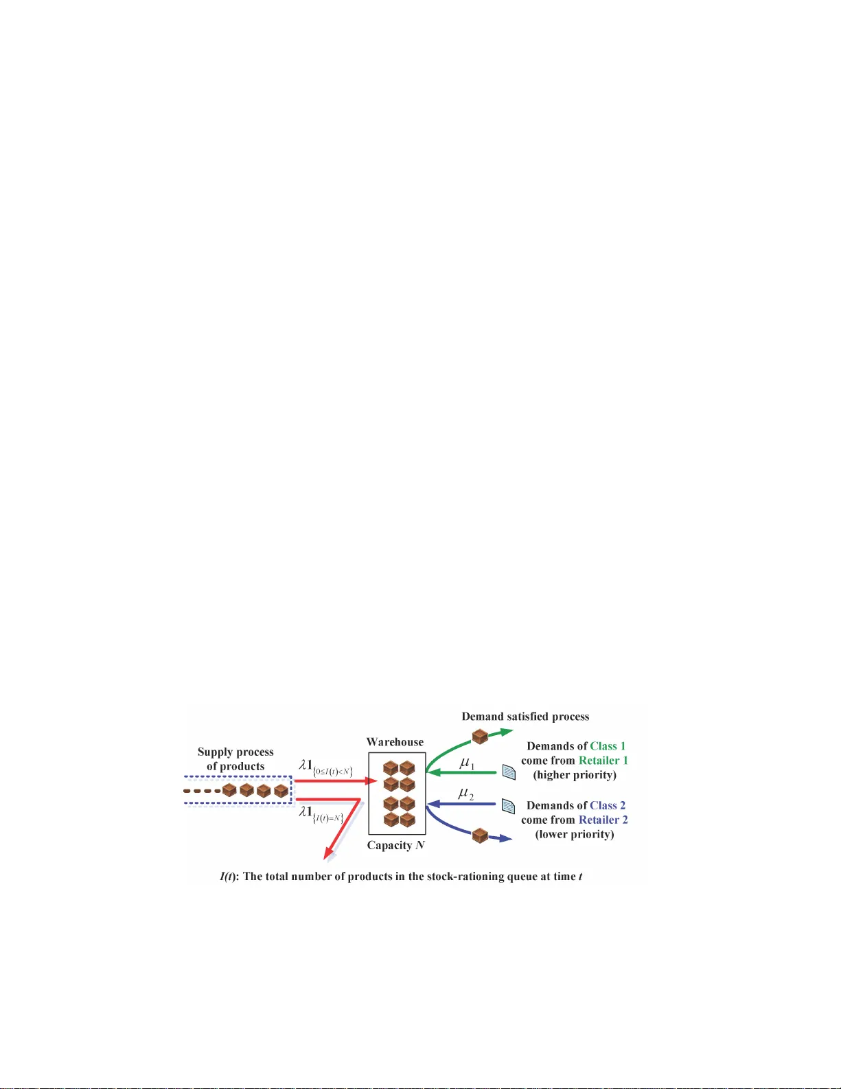
A Complete Algebraic Solution to the Optimal Dynamic Rationing P olicy in the Sto c k-Rationing Queue with Tw o Demand Classes Quan-Lin Li a , Yi-Meng Li b , Jing-Y u Ma b , Heng-Li Liu b a Sc ho ol of E conomics and Managemen t Beijing Univ ersit y of T ec hnology , Beijing 100 124, China b Sc ho ol of Economics and Managemen t Y anshan Univ ersit y , Qinhu angdao 0 66004, China F ebruary 2, 2021 Abstract In this pap er, we study a stock-rationing queue with tw o demand classe s by means of the sensitivity-based optimization, and develop a complete algebr aic solution to the optimal dynamic ratio ning p olicy . W e show that the optimal dynamic ra tio ning po licy m us t be of transfor mational threshold type. Based on this finding, we can refine three sufficient conditions under eac h of whic h the optimal dynamic rationing p o licy is of threshold t yp e (i.e., critical rationing level). T o do this, w e use the performa nce difference eq ua tion to character iz e the monotonicity and optimality of the long- run av erage profit of this sy s tem, a nd thus establish s ome new structural prop erties of the optimal dynamic r ationing p olicy by observing any g iven reference p olicy . Finally , we use n umerical exp eriments to demonstrate our theo retical results of the o ptimal dynamic rationing policy . W e b elieve that the metho do logy and res ults dev elop ed in this paper can shed light on the s tudy of stock-rationing q ueues and open a series of po tent ially promising r e search. Keyw ords: Sto ck-rationing queue; in ven tory rationing; m ultiple demand cla sses; optimal dynamic rationing po licy; se ns itivit y-base d optimization; Mar ko v decision pro cess. 1 1 In tro duction In this pap er, we consider a sto ck- rationing queueing p roblem of a w arehouse w ith one typ e of pro d ucts and t w o classes of demand s, which m a y b e viewed as coming fr om r etailers with t w o differen t priorit y lev els. No w, su c h a stoc k-rationing warehouse s ystem b ecomes more a nd more imp ortant in man y large cities under the current C OVID-19 environmen t. F or exa mple, Beijing h as sev en sup er-large warehouses, which alw a y s su pply v arious daily necessities (e.g., v egetables, m eat, eggs, s eafo o d and so on) to more than 40 million p eople ev ery d a y . In the warehouses, eac h typ e of daily n ecessities are supplied by lots of different companies in C hina and the other coun tries, which lead to that the successiv e su pply stream of eac h type of pro du cts can b e well describ ed as a Poisson pro cess. In addition, the t w o retailers may b e regarded as a large sup ermark et group an d another comm u n it y retail store group. Typicall y , the large sup ermark et group has a higher supply p riorit y th an the comm unit y retail store group. When the COVID-1 9 at Beijing is at a serious w arn in g, the sto c k-rationing managemen t of the warehouses and their optimal sto c k-rationing p olicy pla ys a k ey role in strengthening the fine management of the w arehouses su c h that ev ery family at Beijing can ha v e a v ery comprehensive life guarant ee. F rom the p ersp ectiv e of p ractical applications, such a stoc k-rationing queueing p roblem with multiple demand classes can alwa ys b e encount ered in man y different real areas, for example, assem ble-to-order systems, mak e-to-st o c k queues and multie c helon in ven tory systems b y Ha [39]; multi-ec helon supply c hains by Ragha v an and Roy [75] and Huang and Ir a v ani [44]; manufacturing b y Z hao et al. [95]; military op erations b y K aplan [51]; airline by Lee and Hersh [55]; maritime by J ohn [50 ]; hotel by Bitran and Mond s c hein [8]; r en tal business by P apier and Thonemann [72, 73] and J ain et al. [49]; health care b y Pa pasta vrou et al. [71]; and so f orth . This sho ws that the stock-ratio ning queues with m ultiple demand classes are not only necessary and imp ortan t in man y practical applications, bu t also hav e th eir o wn theoretic al in terest. In the sto ck-rat ioning q u eueing systems, the sto c k rationing p olicies alw ays assign differen t supp ly p r iorities to multiple classes of demands. In the early literature, the so-calle d critic al r ationing level was imagined intuitiv ely , and its existence w as further pro v ed, e.g., see V einott Jr [85] and T opkis [81]. Once the critical rationing lev el is giv en and the on–hand in v en tory falls b elo w th e critica l r ationing lev el, a lo w priorit y demand may b e either rejected, back- ordered or discard ed such that the left on–hand 2 in v en tory will b e reserve d to supp ly the futur e high p riorit y d emands. Th us designing and optimizing the critical rationing lev els b ecomes a basic manag emen t w a y of in v en tory rationing across m ultiple demand classes. So far, analysis of the critical r ationing leve ls has still b een in teresting but d ifficult and c hallenging in the study of sto c k-rationing queues with m ultiple demand classes. Therefore, this motiv ates us in the p ap er to b e interested in the follo wing questions: (P-a) Do es suc h a critical rationing lev el exist? (P-b) If yes, what are the sufficien t (or n ecessary) conditions f or its existence? (P-c) If no, wh ic h useful c h aracteristics can b e furth er found to study th e optimal rationing p olicy? It is interesting and chal lenging to give a complete answer for the ab o v e thr ee problems . F or Problems (P-a) and (P-b) , there h a v e b een some researc h on the the optimal p olicy of critical rationing lev els in in v en tory rationing with m ultiple demand classes. Ho we v er, so far qu ite few stud ies hav e fo cused on Problem (P-c) , since n ob o dy kn o w from wh at p oint o f view and h o w to approac h Problem ( P-c) . F ortunately , this p ap er prop oses and dev elops an algebraic m etho d to b e able to solv e Problem (P-c) . Also, this p ap er u ses the algebraic m etho d to b e able to further deal with P r oblems (P-a) and (P-b) as a sp ecial example. Therefore, this pap er can further sharp en those imp ortan t results giv en in the literature. Differen t from the sub mo dular (or su p ermo dular) tec hnique of the Marko v decision pro cesses (MDPs) devel op ed in the in v en tory rationing literature (e.g., s ee Ha [39, 40, 41]), this pap er app lies the sensitivit y-based optimizatio n to d evelo p an algebraic metho d in the study of sto c k-rationing qu eues with m ultiple d emand classes. The k ey of th e algebraic metho d is to discuss the solutio n P ( d ) i of the linear equatio n G ( d ) ( i ) + b = 0 with resp ect to a basic economic factor (i.e ., price, cost and rew ard), where G ( d ) ( i ) is the p erturb ation realizatio n factor giv en in (31). W e sho w that for an y giv en p olicy d , the solutions P ( d ) i for 1 ≤ i ≤ K pla y a key r ole in solving the ab o v e three problems: (P-a) to (P-c) . See Theorem 10 in Subsection 7.3 for more details. So far some resea rc h h as applied the MDPs to discuss inv en tory rationing (and sto c k- rationing qu eues) across m ultiple d emand classes by means of the su bmo du lar (or sup er- mo dular) tec h nique, among wh ic h imp ortan t examples include Ha [39, 40, 41], Ga y on et al. [37], Benjaafar and ElHafsi [4] and Nadar et al. [67]. T o do this, it is a key th at the structural prop erties of the optimal p olicy need to b e ident ified by using a s et of s truc- 3 tured v alue fun ctions that is preserv ed under an optimal op erator. Based on this findin g, the optimal rationing p olicy of the in v ent ory r ationing across multiple demand cla sses ca n b e further describ ed and expressed b y means of th e s tructural p rop erties. In man y more general cases, it is not easy and eve n v ery diffi cu lt to set u p the structur al prop erties of the optimal p olicy . F or this, some stronger mo del assumptions ha v e to b e further added to guaran tee th e existence of structural prop erties of the optimal p olicy . The purp ose of improvi ng the app licabilit y of the MDPs motiv ates us to prop ose another algebraic metho d in this pap er to d evelo p a complete algebraic solution to the optimal p olicy by means of th e sensitivit y-based optimization. The sens itivit y-based optimization may b e regarded as a new r esearc h branch of the MDPs, whic h gro ws out of infin itesimal p erturbation analysis of discrete ev en t dynamic systems, e.g., see Cao [10, 11]. Note that one key of the sensitivit y-based optimiza tion is to set up and u se the so-called p erformance differen ce equation, which is based on the p ertur b ation realizat ion factor as we ll as the p erformance p otent ial related to the Po isson equation. T o the b est of our kn o wledge, this p ap er is the fi r st to apply the sens itivity- based optimization to study the sto c k-rationing queues with multiple demand classes. On suc h a researc h line, there are only a few closely relate d works in the recen t literature, for example, the energy-efficien t d ata cent ers b y Ma et al. [60] and the group-serv er queues by Xia et al. [92]. Different from Ma et al. [60] and Xia et al. [92], this p ap er dev elops a complete algebraic solution to the optimal dynamic rationing p olicy of the sto c k-rationing queue with m ultiple demand classes, and sho ws that the optimal dyn amic rationing p olicy m ust b e of transformational thresh old typ e, wh ic h can lead to r efining three sufficient conditions un der eac h of whic h the op timal d ynamic rationing p olicy is of threshold t yp e (see Th eorem 10 in Sub s ection 7.3). In addition, it is w orth while to note that our transformational thresh old t yp e results are sharp er than th e b ang-bang con trol giv en in Ma et al. [60], Xia et al. [92] and others. Therefore, our algebraic metho d pro vides n ot only a necessary complement of p olicy sp atial structural integ rit y bu t also a new wa y of optimalit y pro ofs when comparing to the fr equ en tly-used sub mo dular (or sup er m o dular) tec hnique of MDPs. Also, the complete algebraic solution to the optimal dynamic rationing p olicy can pro vide more effectiv e supp ort for numerical computation of the optimal p olicy and the optimal profit of this system. Note that the Poisson equations alw a ys play a k ey role in the study of MDPs. T o the b est of our kno wledge, this pap er pro vides a new general solutio n with t w o fr ee constants: 4 A p oten tial d isplacemen t constant, and another solution-free constan t (see Th eorem 1 in Section 5). In addition, it is clear that s u c h a general solution of the P oisson equations can b e further extended and generalized to a blo ck structur e of more general mo dels by means of the R G-factorizatio ns (see Li [56]). F or the Poisson equations, readers may refer to, suc h as Bh ulai [6], Ma k o wski and Shw artz [61], Asmussen and Bladt [3], Bini et al. [7] and Ma et al. [60] for more details. Based on the ab o v e analysis, we summarize the main cont ributions of this pap er as follo ws : (1) A c omplete algebr aic solution: W e study a sto ck-rati oning qu eue with t w o demand classes by means of the sens itivit y-based optimization, and pro vide a complete al- gebraic s olution to the optimal dynamic ratio ning p olicy . W e first sh ow th at the optimal dynamic p olicy must b e of transformational th reshold typ e. Then we refi n e three suffi cien t conditions und er eac h of whic h the optimal d ynamic rationing p olicy is of thr eshold t yp e. S ee Theorem 10 in Subsection 7.3 for details. (2) A unifie d c omputatio nal fr amework: T o the b est of ou r kno wledge, this pap er is the first to apply the sensitivit y-based optimization to analyze the sto c k-rationing queues with m ultiple d emand classes. Thus it is n ecessary and useful to describ e the three k ey steps: (a) Setting u p a p olicy-based Mark o v p ro cess. (b) Constructing a p olicy-based P oisson equ ation, whose general solution can b e used to c haracterize the m onotonicit y and optimalit y of the long-run av erage p rofit of this system. (c) Finding the optimal dyn amic rationing p olicy in the three differen t areas of the p enalt y cost. In addition, th e computational framew ork can sufficient ly supp ort n umerical solutio n of sto c k-rationing queues with m u ltiple d emand classes while the submo d ular (or sup ermo dular) tec hnique of MDPs is ve ry difficult to deal with more general sto ck-rati oning queues. (3) A difficult ar e a of the p enalty c ost is solve d: I n our algebraic m etho d, it is a ke y to set up a linear equation: G ( d ) ( i ) + b = 0 in the p enalt y cost P f or 1 ≤ i ≤ K . W e sho w that the solution P ( d ) i of G ( d ) ( i ) + b = 0 for 1 ≤ i ≤ K pla ys a key role in finding the optimal dynamic rationing p olicy . By using the solution P ( d ) i for 1 ≤ i ≤ K , t wo k ey indices P L ( d ) and P H ( d ) are defined in (46) and (47) suc h that the range of th e p enalt y cost P is divided into three different areas: (a) P ≥ P H ( d ); 5 (b) P L ( d ) > 0 and 0 < P ≤ P L ( d ); and (c) P L ( d ) < P < P H ( d ). In th e fir st t w o areas, w e sho w that the optimal d ynamic rationing p olicy is of threshold t yp e; while for the third area, it is more difficult to analyze the optimal dyn amic rationing p olicy so that the b an g-bang con trol is alwa ys su ggested as a r ou gh result for this case in the literature, e.g., see Ma et al. [60] and Xia et al. [92]. Unlik e those, this pap er pro vides a detailed analysis for the d ifficult area: P L ( d ) < P < P H ( d ), c haracterizes the monotonicit y and optimalit y of the long-run a v erage profit of this system, and fu rther establish some new structur al prop erties of the optimal dyn amic rationing p olicy by observing any giv en r eference p olicy . Th is leads to a complete algebraic solution to the optimal d ynamic rationing p olicy . (4) Two differ ent metho ds c an sufficiently supp ort e ach other: Note that our alg ebraic metho d sets up a complete algebraic solution to the optimal dynamic rationing p ol- icy , th us it can pro vide not only a necessary complemen t of p olicy spatial structural in tegrit y bu t also a new w a y of optimalit y pro ofs w hen comparing to the frequent ly- used submo d ular (or sup ermo du lar) tec hnique of MDPs. O n the other hand , s ince our algebraic metho d and the su bmo du lar (or sup erm o dular) tec hnique are all im- p ortant p arts of the MDPs (the former is to u se the p oisson equations; wh ile the latter is to apply the optimalit y equ ation), it is clear that the tw o d ifferen t meth- o ds will sufficien tly supp ort eac h other in the study of stock-rat ioning qu eues (and rationing inv ento ry) with multiple demand classes. The remainder of this pap er is organized as follo w s. Section 2 provides a literature review. Section 3 giv es mo del description for the sto ck-rat ioning queue with tw o demand classes. Section 4 establishes an optimizat ion problem to fi nd the optimal dynamic ra- tioning p olicy , in which we set up a p olicy-based bir th-death pro cess and define a more general rew ard function. Section 5 establishes a p olicy-based Poisson equ ation and pro- vides its general solution with t w o fr ee constant s. Section 6 provi des an explicit expression for the p erturbation realiza tion f actor G ( d ) ( i ), and discusses the solution of the linear equation G ( d ) ( i ) + b = 0 in the p enalt y cost P for 1 ≤ i ≤ K . Section 7 d iscusses the monotonicit y and optimalit y of th e long-run a v erage profit of this sys tem, and finds th e optimal dyn amic rationing p olicy in three different areas of the p enalt y cost. Section 8 analyzes the stoc k-rationing queue un d er a threshold t yp e (statical) r ationing p olicy . Sec- tion 9 uses numerical exp eriments to demonstrate our theoretical results of the optimal 6 dynamic rationing p olicy . Finally , some concluding r emarks are give n in Section 10. 2 Literature Review Our current researc h is r elated to three literature streams: T he first is the research on sto c k-rationing queues, critical rationing lev els an d their MDP p r o ofs. The second is on the static rationing p olicy and the dynamic rationing p olicy in in v en tory rationing across m ultiple d emand classes. The th ird is on a s imple introdu ction to the sensitivit y-based optimization. The inv en tory r ationing across multiple demand classes w as fir st analyzed b y V einott Jr [85] in the con text of in v en tory control theory . F rom then on, some auth ors h a v e discussed the in v en tory rationing problems. So far suc h in v ent ory rationing has still been in teresting and c hallenging. Readers ma y refer to a b o ok by M¨ ollering [64]; su r v ey pap ers b y K leijn and Dekk er [52] and Li et al. [59]; and a researc h classification b y T eunter and Hanev eld [80], M¨ olle ring and Thon emann [65], V an F oreest and Wijngaard [83] and Alfi eri et al. [1]. (a) St o c k-rationing queues, critical rat ioning levels and their MDP pro ofs In a rationing in v en tory sys tem, a critical r ationing lev el w as imagined from early researc h and practical exp erience. V einott Jr [85] first prop osed suc h a critical rationing lev el; while T opkis [81] prov ed that the critical rationing lev el really exists and it is an optimal p olicy . Similar results we re fur th er develo p ed f or tw o demand classes by Ev ans [33] and Kaplan [51]. It is a most basic problem ho w to mathematically pro v e wh ether a rationing inv en tory system has suc h a critical rationing lev el. Ha [39] made a breakthrough by applyin g the MDPs to analyze the inv entory rationing p olicy for a sto ck-rat ioning qu eu e with exp onenti al pro duction times, Poi sson d emand arriv als, lost sales and m u ltiple demand classes. He prov ed that th e optimal rationing p olicy is of critical rationing lev els, and sho w ed that not only d o the critic al rationing levels exist, but also they are monotone and stati onary . Therefore, the optimal rationing p olicy was charac terized as a monotone constan t sequence of critical r ationing lev els corresp onding to the multiple d emand classes. Since th e seminal w ork of Ha [39], it has b een in teresting to extend and generalize the wa y to apply th e MDPs to d eal w ith the sto c k-rationing queues and the ratio ning 7 in v en tory systems. Imp ortant examples includ e the Erlang pro d uction times by Ha [41] and Ga y on et al. [37]; the bac k orders with t w o demand classes by Ha [40] and with multiple demand classes by d e V´ ericourt [19, 20]; the parallel pr o duction c hannels by Bulu t and F adilo˘ g lu [9]; the batc h ordering by Huang and Ira v ani [45], th e batc h pro duction b y P ang et al. [70]; the utilization of information b y Ga y on et al. [36] and ElHafsi et al. [29]; an assem ble-to-order p ro du ction system by Benjaafar and ElHafsi [4], ElHafsi [27], ElHafsi et al. [28, 30], Benjaafar et al. [5] and Nadar et al. [67]; a tw o-stage tandem pro d uction system by Xu [93], sup p ly chain b y Huang and Ira v ani [44] and v an Wijk et al. [84]; p erio dic review b y F rank et al. [35 ] an d Chen et al. [15]; dyn amic pr ice b y Ding et al. [24, 25], Sch u lte and Pib ernik [76]; and so forth. Differen t from those works in th e literature, this pap er applies the sensitivit y-based optimization to study a sto c k-rationing q u eue with t w o d emand classes, and provides a complete algebraic solution to the optimal dyn amic rationing p olicy . T o this end, this pap er fi rst sho ws that the optimal d ynamic p olicy must b e of transf ormational thresh old t yp e. Then it refines three sufficient cond itions under eac h of whic h the optimal d ynamic rationing p olicy is of thr eshold t yp e. In addition, this pap er uses th e p erf orm ance dif- ference equation to charact erize the monotonicit y and optimalit y of th e long-run a ve rage profit of this system, and establish some n ew structural pr op erties of th e optimal dynamic rationing p olicy b y observing any giv en r eferen ce p olicy . (b) I n v en tory rationing across m ultiple demand classes In the inv entory rationing literature, th er e exist t w o kin d s of rationing p olicies: The static r ationing p olicy , and the dynamic rationing p olicy . Note that the dynamic r ationing p olicy allo ws a threshold rationing level to b e able to c hange in time, dep end ing on the n umber and ages of outstand in g ord ers. In general, the static rationing p olicy is p ossible to miss some c hances to fur ther imp r o v e system p erformance, while the dynamic r ationing p olicy s hould r eflect b etter by means of v arious con tin uously up dated inf orm ation, the system p erformance can b e impr ov ed dynamically . Deshpand e et al. [23] indicated that the optimal dynamic rationing p olicy m a y signifi can tly red u ce the inv entory cost compared with the static rationing p olicy . If there exist multiple replenish men t opp ortu n ities, then th e ord ering p olicies are tak en as tw o differen t t yp es: P erio dic review and con tin uous review. Therefore, our literature analysis for in v en tory rationing fo cuses on four different classes throu gh com b ining th e 8 rationing p olicy (static v s . dynamic) w ith the inv entory review (con tinuous v s . p erio d ic) as follo w s: Static-con tinuous, static- p erio dic, dyn amic-con tin uous, and dynamic-p erio dic. (b-1) The static r ationing p olicy (p e rio dic vs. c ontinuous) The p erio dic r eview: V einott Jr [85] is the first to intro d uce an inv entory rationing across different d emand classes and to prop ose a critical ratio ning level (i.e., the static rationing p olicy) in a p erio d ic review inv entory system with b ac korders. Subsequent r e- searc h fu rther inv estigated the p erio dic review inv ento ry system with m ultiple demand classes, for example, th e ( s, S ) p olicy by C ohen et al. [18] and T emp elmeier [79]; the ( S − 1 , S ) p olicy by d e V ´ ericourt [20] and Ha [39, 40]; the lost sales by Dekk eret et al. [21]; the bac korders by M¨ ollering and Th onemann [65]; and the an ticipated cr itical lev els b y W ang et al. [88]. The c ontinuous r evie w: Nahmias and Demm y [68] is the first to prop ose and dev elop a constant critical lev el ( Q, r , C ) p olicy in a con tin uous review in v en tory mo d el with m ultiple demand classes, wh er e Q is the fi x ed batc h size, r is the reorder p oin t and C = ( C 1 , C 2 , . . . , C n − 1 ) is a set of critical rationing lev els for n demand cla sses. F rom that time on, some authors hav e d iscussed the constant critical lev el ( Q, r, C ) p olicy in con tin uous r eview inv entory systems. Readers ma y r efer to recen t p u blications for details, among wh ic h are Melc hiors et al. [63], Dekk eret et al. [22], Deshpande et al. [23], Isotupa [48], Arslan et al. [2 ], M¨ ollering and Th onemann [65, 66] and Escalona et al. [32, 31]. In addition, the ( S − 1 , S, C ) in v en tory sy s tem was discussed by Dekk eret et al. [21], Kranenburg and v an Houtum [53] and so on. (b-2) The dynamic r ationing p olicy (c ontinuous vs. p e rio dic) The c ontinuous r eview: T opkis [81] is the first to analyze the dynamic rationing p ol- icy , and to indicate that the optimal r ationing p olicy is a dynamic p olicy . Ev ans [33] and Kaplan [51] obtained similar results as that in T opkis [81] for tw o demand classes. Melc hiors [62] considered a dynamic rationing p olicy in a ( s, Q ) in ven tory system w ith a key assumption that there was at m ost one outstanding ord er. T eunter and Haneveld [80] dev elop ed a cont inuous time approac h to d etermin e the dynamic rationing p olicy for t w o Poisson demand classes, analyz ed the marginal cost to d etermine the optimal remain- ing time for eac h rationing leve l, and expr essed the optimal threshold p olicy through a sc hematic d iagram or a lo okup table. F adılo˘ glu and Bulut [34] prop osed a dynamic ra- tioning p olicy: R ationing with Exp onen tial R ep lenishment Flo w (RERF), for con tin uous review inv entory systems with either bac k orders or lost sales. W an g et al. [87] dev elop ed 9 a dyn amic threshold mec hanism to allo cate bac korders when the m ultiple outstanding orders for d ifferen t demand classes exist for th e ( Q, R ) inv entory system. The p erio dic r eview: F or the dyn amic r ationing p olicy in a p erio d ic review inv ento ry system, readers ma y refer to, suc h as t w o demand classes b y Sob el and Zhang [77], F rank et al. [35] and T an et al. [78]; dynamic critical lev els and lost sales by Ha ynsw orth and Price [42]; multiple demand classes by Hung and Hsiao [47]; tw o bac k order classes b y Chew et al. [17]; general demand p ro cesses b y Hun g et al. [46]; mixed bac k orders and lost sales by W ang and T ang [86]; uncertain demand and pro du ction rates by T urga y et al. [82]; and in cr emental upgradin g demand s b y Y ou [94]. (c) The sensitivity-based optimization In the early 1980s, Ho and Cao [4 3] pr op osed and dev elop ed infinitesimal p ertu rbation metho d of discrete even t dynamic systems (DEDSs), whic h is a n ew researc h direction for online s im ulation optimization of DEDSs sin ce the 1980s. Readers ma y refer to the excellen t b o oks b y , suc h as Cao [10], Glasserman [38] and C assandras and Lafortune [14]. Cao et al. [13] and Cao and Chen [12] publish ed a seminal wo rk that transforms the infin itesimal p erturb ation, together with the MDPs and th e reinforcement learnin g, in to the sensitivit y -b ased optimization. On this researc h line, the excellen t b o ok b y Cao [11] s u mmarized the main resu lts in the stud y of sensitivit y-based optimization. Li and Liu [58] and C hapter 11 in L i [56 ] further extended and generalize d the sensitivit y-based optimization to a m ore general fr amew ork of p ertu rb ed Mark o v pro cesses. In addition, the sen sitivit y-b ased optimizati on can b e effectiv ely deve lop ed by means of the matrix- analytic m etho d by Neuts [69], Latouche and Ramasw ami [5 4], and the R G-facto rizations of blo ck-structured Mark o v p ro cesses by Li [56] and Ma et al. [60]. So far some researc h has applied the sensitivit y-b ased optimization to analyze th e MDPs of qu eues and net wo rks, e.g., see Xia and C ao [89], Xia and Shihada [91], Xia et al. [90, 92], Ma et al. [60] and a surve y pap er b y Li et al. [59]. Finally , to the b est of our knowle dge, this pap er is th e first to ap p ly the sensitivit y- based optimization to analyze the sto ck-rati oning queues w ith m ultiple demand classes. Our algebraic metho d sets up a complete algebraic solution to the optimal d ynamic ra- tioning p olicy , thus it p ro vides not only a necessary complemen t of p olicy sp atial structural in tegrit y b ut also some new pro ofs of monotonicit y and optimalit y . Note that our alge- 10 braic m etho d and the subm o dular (or sup ermo dular) tec h nique are all imp ortan t parts of the MDPs. The former is to mainly u se the p oisson equations, w hic h are w ell related to Mark o v (reward) pro cesses; while the latter is to fo cus on the optimalit y equation b y applying the monotonous op erator theory to p ro v e the optimalit y . Therefore, it is clear that the t w o different metho ds can sufficien tly su pp ort eac h other in the stud y of sto c k- rationing queues with m u ltiple demand classes. W e b eliev e that the metho dology an d results dev elop ed in this pap er can b e app licable to the study of sto c k-rationing qu eues and op en a series of p oten tially promising researc h. 3 Mo d el Description In this section, we d escrib e a sto ck- rationing queue with tw o demand classes, in which a single class of p ro ducts are supp lied to stock at a warehouse, and the t wo classes of demands come f rom t wo reta ilers with differen t priorities. In addition, w e provide system structure, op er ational mo de and mathematical notatio ns. A sto c k-rationing queue: The w arehouse h as the maximal capacit y N to sto c k a single class of pr o ducts, and the wa rehouse needs to pa y a holdin g cost C 1 p er pro duct p er unit time. Th er e are tw o classes of demands to order the pro ducts, in whic h the d emands of Class 1 hav e a higher priority than that of Class 2, suc h that th e demands of Class 1 can b e satisfied in any non-zero inv entory; while the demands of Class 2 may b e either satisfied or refused based on the in v en tory lev el of the pro ducts. Figure 1 depicts a simple physic al system to und er s tand the sto c k-rationing qu eue. Figure 1: A sto ck- rationing queue with t wo demand classes The supply process : The su pply s tream of the pro du cts to the wa rehouse is a Poisson 11 pro cess with arriv al rate λ , where the price of p er pro du ct is C 3 paid by the warehouse to the external pro d uct supp lier. If th e wa rehouse is full of the pro d u cts, then an y new arriving pro du ct has to b e lost . I n this ca se, th e warehouse w ill h a v e an opp ortunity cost C 4 p er pro duct rejected int o the w arehouse. The service pro cesses: The service times p ro vided b y the w arehouse to satisfy th e demands of Classes 1 and 2 are i.i.d. and exp on ential with service rates µ 1 and µ 2 , resp ectiv ely . The serv ice disciplines for the t wo classes of d emands are all First Come First S erv e (F CFS). The w arehouse can obtain the service price R when one p ro duct is sold to Retailer 1 or 2. Note that eac h demand of Class 1 or 2 is satisfied b y one pro du ct ev ery time. The sto ck-rationing rule : F or the t wo classes of demands, eac h demand of Class 1 can alw a ys b e satisfied in an y non-zero inv ent ory; while for satisfying the demands of Class 2, we need to consider three different cases as follo ws: Case one : The inventory level is zer o. In this case, there is no pro d uct in the ware- house. Thus an y new arriving demand has to b e rejected imm ediately . Th is leads to the the lo st sales cost C 2 , 1 (resp. C 2 , 2 ) p er unit time for any lost demand of Class 1 (resp. 2). W e assume that C 2 , 1 > C 2 , 2 , w hic h is used to guaran tee the higher priorit y service for the demands of C lass 1 wh en comparing to the low er priorit y for th e demand s of Class 2. Case two : The inventory level is low. In this case, the n um b er of p ro ducts in th e w arehouse is not m ore than a key th reshold K , where the threshold K is sub jectiv ely designed b y means of some r eal exp erience. Note that the demands of Class 1 ha ve a higher priority to receiv e the pro d ucts than the demands of C lass 2. Thus the w areh ou s e will not provide an y pro du ct to satisfy the demands of Class 2 un der an equal service condition if the num b er of pro ducts in the w arehouse is not more than K . Otherwise, suc h a service priorit y is violated (i.e., the demands of Class 2 are satisfied from a lo w sto c k), so that the warehouse m ust pa y a p enalt y cost P p er pro duct sup p lied to the demands of C lass 2 at a lo w sto c k. Note that the p enalt y cost P measures d ifferen t priorit y level s to provide the pro du cts b et w een the tw o classes of demands. Case thr e e : The inventory level is high. In this case, the num b er of p ro ducts in th e w arehouse is more than the thresh old K . Thus the demand s of Classes 1 and 2 can b e sim ultaneously satisfied thanks to enough pro ducts in the w arehouse. Indep endence: W e assume that all the random v ariables defined ab ov e are in dep en- den t of eac h other. 12 In what follo ws, w e u s e T able 1 to further sum marize some ab ov e notat ions. T able 1: S ome costs and prices in the sto c k-rationing queue C 1 The holding cost p er unit time p er pro duct stored in the w arehouse C 2 , 1 The lost sales cost of eac h lost demand of Class 1 C 2 , 2 The lost sales cost of eac h lost demand of Class 2 C 3 The price of p er pro duct paid b y the warehouse to the external pr o duct supplier C 4 The opp ortun it y cost p er pro du ct rejected in to the warehouse P The p enalty cost p er pro duct sup plied to the demands of Class 2 at a low stock R The service price of the w arehouse paid b y eac h satisfied demand 4 Optimization Mo del F orm ulation In this section, we establish an optimization problem to fi nd the optimal dynamic rationing p olicy in the sto ck-ratio ning queue. T o d o this, w e set up a p olicy-based birth-d eath pro cess, and d efi ne a m ore general reward function w ith resp ect to b oth states and p olicies of the p olicy-based birth -d eath pro cess. T o study the sto c k-rationing queue with tw o demand classes, we first need to define b oth ‘states’ and ‘p olicies’ to exp ress sto c hastic dynamics of the sto ck-ratio ning queue. Let I ( t ) b e the n um b er of prod ucts in the w arehouse at time t . Th en it is regarded as the sta te of this system at time t . O b viously , all the cases of S tate I ( t ) form a state space as follo ws: Ω = { 0 , 1 , 2 , . . . , N } . Also, State i ∈ Ω is regarded as an in v en tory leve l of this sys tem. F rom the states, some p olicies are defi ned with a little b it more complexit y . Let d i b e a p olicy related to State i ∈ Ω , and it expresses whether or not the warehouse prefers to su pply some pro d ucts to the demands of Class 2 wh en the in v en tory lev el is not more than the threshold K for 0 < K ≤ N . Thus, w e ha v e d i =        0 , i = 0 , 0 , 1 , i = 1 , 2 , . . . , K, 1 , i = K + 1 , K + 2 , . . . , N , (1) 13 where d i = 0 and 1 represent s that the wa rehouse rejects and satisfies the demands of Class 2, resp ectiv ely . Ob viously , n ot only d o es the p olicy d i dep end on State i ∈ Ω , but also it is controlle d b y the threshold K . Of course, for a sp ecial case, if K = N , then d i ∈ { 0 , 1 } for 1 ≤ i ≤ N . Corresp ond ing to eac h state in Ω , we defin e a time-homogeneo us p olicy of the sto c k- rationing queue as d = ( d 0 ; d 1 , d 2 , . . . , d K ; d K +1 , d K +2 , . . . , d N ) . It follo w s from (1) that d = (0; d 1 , d 2 , . . . , d K ; 1 , 1 , . . . , 1) . (2) Th us Poli cy d dep ends on d i ∈ { 0 , 1 } , whic h is r elated to State i for 1 ≤ i ≤ K . L et all the p ossible p olicies of the sto c k-rationing queue, giv en in (2), form a p olicy sp ace as follo ws : D = { d : d = (0; d 1 , d 2 , . . . , d K ; 1 , 1 , . . . , 1) , d i ∈ { 0 , 1 } , 1 ≤ i ≤ K } . Remark 1 In gener al, the thr eshold K is subje ctive and is designe d by me ans of the r e al exp erienc e of the war ehouse manager. If K = N , then the p olicy i s expr esse d as d = (0; d 1 , d 2 , . . . , d N ) . Thus our K -b ase d p olicy d = (0; d 1 , d 2 , . . . , d K ; 1 , 1 , . . . , 1) is mor e gener al than Policy d = (0; d 1 , d 2 , . . . , d N ) . Let I ( d ) ( t ) b e the state of the stock-rati oning qu eue at time t un der any giv en p olicy d ∈ D . Then  I ( d ) ( t ) : t ≥ 0  is a con tin uous-time p olicy-based Mark o v pro cess on th e state space Ω whose state transition relatio ns are depicted in Figure 2. 0 O 1 2 P P  1 O 2 O K O O K+ 1 . . . 1 2 K d P P  1 3 2 d P P  1 2 2 d P P  1 1 2 d P P  O N -1 O O N . . . 1 2 P P  1 2 P P  1 2 P P  Figure 2: State trans ition relations of the p olicy-based Mark o v pro cess 14 It is easy to see from Figure 2 that  I ( d ) ( t ) : t ≥ 0  is a p olicy-based birth-death pro cess. Based on this, the in finitesimal g enerator of the p olicy-based birth-death pro cess  I ( d ) ( t ) : t ≥ 0  is giv en b y B ( d ) =                    − λ λ v ( d 1 ) − [ λ + v ( d 1 )] λ . . . . . . . . . v ( d K ) − [ λ + v ( d K )] λ v (1) − [ λ + v (1)] λ . . . . . . . . . v (1) − [ λ + v (1) ] λ v (1) − v (1)                    , (3) where v ( d i ) = µ 1 + d i µ 2 for i = 1 , 2 , . . . , K , and v (1) = µ 1 + µ 2 . It is clear that v ( d i ) > 0 for i = 1 , 2 , . . . , K . Thus the p olicy-based birth-d eath pro cess B ( d ) m ust b e irr educible, ap erio dic and p ositiv e recurr ent for any giv en p olicy d ∈ D . In this case, we write the stationary p robabilit y v ector of the p olicy-based birth-death pro cess  I ( d ) ( t ) : t ≥ 0  as π ( d ) =  π ( d ) (0); π ( d ) (1) , . . . , π ( d ) ( K ); π ( d ) ( K + 1) , . . . , π ( d ) ( N )  . (4) Ob viously , th e stationary probabilit y v ector π ( d ) is the unique solution to the system of linear equations: π ( d ) B ( d ) = 0 and π ( d ) e = 1, where e is a column v ector of ones with a suitable dimens ion. W e wr ite ξ 0 = 1 , i = 0 , ξ ( d ) i =            λ i i Q j =1 v ( d j ) , i = 1 , 2 , . . . , K , λ i ( µ 1 + µ 2 ) i − K K Q j =1 v ( d j ) , i = K + 1 , K + 2 , . . . , N , (5) and h ( d ) = 1 + N X i =1 ξ ( d ) i . It follo w s from Subs ection 1.1.4 of Ch apter 1 in Li [56] that π ( d ) ( i ) =    1 h ( d ) , i = 0 1 h ( d ) ξ ( d ) i , i = 1 , 2 , . . . , N . (6) 15 By usin g the p olicy-based birth-d eath pro cess B ( d ) , now w e define a more general rew ard function in the sto c k-rationing queue. It is seen f r om T able 1 that the rew ard function w ith r esp ect to b oth states and p olicies is defined as a profit r ate (i.e. the total system rev en ue minus the total system cost p er unit time). By observing the impact of P olicy d on the profit r ate, the reward function at S tate i un der P olicy d is giv en by f ( d ) ( i ) = R  µ 1 1 { i> 0 } + µ 2 d i  − C 1 i − C 2 , 1 µ 1 1 { i =0 } − C 2 , 2 µ 2 (1 − d i ) − C 3 λ 1 { i 0 } and 1 { i =0 } , resp ectiv ely; the exte rnal pro d ucts en ter or are lost by the warehouse according to 1 { i 0. Let H ( d ) and ϕ ( d ) b e t wo column v ectors of size N obtained th r ough omitting the fi rst elemen ts of the tw o column vecto rs f ( d ) − η d e and g ( d ) of size N + 1, resp ectiv ely . T hen, H ( d ) =                  H ( d ) 1 H ( d ) 2 . . . H ( d ) K H ( d ) K +1 . . . H ( d ) N                  =                  f ( d ) (1) − η d f ( d ) (2) − η d . . . f ( d ) ( K ) − η d f ( K + 1) − η d . . . f ( N ) − η d                  =                  h B ( d ) 1 − D ( d ) i − P h A ( d ) 1 − F ( d ) i h B ( d ) 2 − D ( d ) i − P h A ( d ) 2 − F ( d ) i . . . h B ( d ) K − D ( d ) i − P h A ( d ) K − F ( d ) i  B K +1 − D ( d )  − P  A K +1 − F ( d )  . . .  B N − D ( d )  − P  A N − F ( d )                   and ϕ ( d ) =  g ( d ) (1) , g ( d ) (2) , . . . , g ( d ) ( K ) ; g ( d ) ( K + 1) , g ( d ) ( K + 2) , . . . , g ( d ) ( N )  T . 22 Therefore, it follo ws from (26) that − B ϕ ( d ) = H ( d ) + ν ( d 1 ) e 1 g ( d ) (0) , (27) where e 1 is a column v ector with th e first elemen t b e on e and all the others b e zero. Note that the matrix −B is inv ertible and ( −B ) − 1 > 0, thus the system of linear equ ations (27) alw a ys has one unique solution ϕ ( d ) = ( −B ) − 1 H ( d ) + ν ( d 1 ) ( −B ) − 1 e 1 · ℑ , (28) where g ( d ) (0) = ℑ is an y giv en constan t. Let’s tak e a con ven tion   a b   = ( a, b ) T , where b may b e a column v ector. Then we ha ve g ( d ) =  g ( d ) (0) , ϕ ( d )  T =  ℑ , ( −B ) − 1 H ( d ) + ν ( d 1 ) ( −B ) − 1 e 1 · ℑ  T =  0 , ( −B ) − 1 H ( d )  T +  1 , ν ( d 1 ) ( −B ) − 1 e 1  T ℑ . (29) Note that B ( d ) e = 0 , th us a general solution to the p olicy-based Po isson equation is further giv en by g ( d ) =  0 , ( −B ) − 1 H ( d )  T +  1 , ν ( d 1 ) ( −B ) − 1 e 1  T ℑ + ξ e , (30) where ℑ and ξ are t wo free constan ts. Based on the ab o ve analysis, the f ollo win g theorem sum m arizes the general solution of the p olicy-based Po isson equation. Theorem 1 F or the P oisson e quation − B ( d ) g ( d ) = f ( d ) − η d e , ther e exists a key sp e cial solution g d Sp =  0 , ( −B ) − 1 H ( d )  T , and its gener al solution is r elate d to two fr e e c onstants ℑ and ξ such that g ( d ) = g d Sp +  1 , ν ( d 1 ) ( −B ) − 1 e 1  T ℑ + ξ e , wher e ξ is a p otential displac ement c onstant, and ℑ is a solution-fr e e c onstant. Remark 2 (1) T o our b est know le dge, this is the first to pr ovide the ge ner al solution of the Poisson e quations in the MDPs by me ans of two differ ent fr e e c onstants. 23 (2) Note that π ( d ) g ( d ) = η d and the matrix − B ( d ) + e π ( d ) is invertible, thus the Poisson e quation − B ( d ) g ( d ) = f ( d ) − η d e c an b e c ome  − B ( d ) + e π ( d )  g ( d ) = f ( d ) . This gives a solution of the Poisson e quation as fol lows: g ( d ) =  − B ( d ) + e π ( d )  − 1 f ( d ) + ξ e , which is a sp e cial solution of the Poisson e quation by c omp aring with that in The or em 1. 6 Impact of the P enalt y Cost In th is sec tion, we provide an explicit expr ession for the p erturbation real ization factor of the p olicy-based birth-death pro cess. Based on this, we can set up a linear equation in th e p enalt y cost, which is w ell related to the p erform ance difference equation. F urtherm ore, w e discuss some useful prop erties of p olicies in the set D by means of the solution of the linear equation in the p enalt y cost. 6.1 The p erturbation r ealization factor W e d efine a p erturbation realizatio n factor as G ( d ) ( i ) def = g ( d ) ( i − 1) − g ( d ) ( i ) , i = 1 , 2 , . . . , N . (31) It is easy to see from Cao [11] that G ( d ) ( i ) quan tifies the difference among t wo adjacen t p erformance p oten tials g ( d ) ( i ) and g ( d ) ( i − 1) , and measures the effect on the long-run a v erage profit of the stock-ratio ning queue when the system s tate is c hanged from State i − 1 to State i . By using the p olicy-based P oisson equation (26), we can derive a new system of linear equ ations, whic h can b e u s ed to directly express the p erturb ation realizat ion factor G ( d ) ( i ) for i = 1 , 2 , . . . , N . By using (30), w e can directly express the p erturbation realizatio n factor G ( d ) ( i ) for i = 1 , 2 , . . . , N . On the other hand, b y observing the sp ecial structure of the p olicy-based P oisson equation (26), we can pr op ose a new m etho d of sequence to set u p an explicit expression for G ( d ) ( i ). F or i = 1, it follo ws from (22) th at − λ h g ( d ) (0) − g ( d ) (1) i = − λG ( d ) (1) , 24 w e hav e λG ( d ) (1) = f ( 0) − η d . (32) F or i = 2 , 3 , . . . , K , it follo ws from (23) that v ( d i ) h g ( d ) ( i − 1) − g ( d ) ( i ) i − λ h g ( d ) ( i ) − g ( d ) ( i + 1) i = v ( d i ) G ( d ) ( i ) − λG ( d ) ( i + 1) , this giv es λG ( d ) ( i + 1) = v ( d i ) G ( d ) ( i ) + f ( d ) ( i ) − η d . (33) F or i = K + 1 , K + 2 , . . . , N − 1, it follo ws fr om (24) that ( µ 1 + µ 2 ) h g ( d ) ( i − 1) − g ( d ) ( i ) i − λ h g ( d ) ( i ) − g ( d ) ( i + 1) i = ( µ 1 + µ 2 ) G ( d ) ( i ) − λG ( d ) ( i + 1) , w e obtain λG ( d ) ( i + 1) = ( µ 1 + µ 2 ) G ( d ) ( i ) + f ( i ) − η d . (34) F or i = N , it follo ws from (25) that ( µ 1 + µ 2 ) G ( d ) ( N ) = η d − f ( N ) . (35) By using (32), (33), (34) and (35 ), w e obtai n a new system of linear equations satisfied b y G ( d ) ( i ) as follo ws:              λG ( d ) (1) = f (0) − η d , i = 1 , λG ( d ) ( i + 1) = v ( d i ) G ( d ) ( i ) + f ( d ) ( i ) − η d , i = 2 , 3 , . . . , K, λG ( d ) ( i + 1) = ( µ 1 + µ 2 ) G ( d ) ( i ) + f ( i ) − η d , i = K + 1 , K + 2 , . . . , N − 1 , ( µ 1 + µ 2 ) G ( d ) ( N ) = η d − f ( N ) , i = N . (36) F ortunately , th e follo wing theorem can pr o vide an exp licit expression for the p ertur- bation realization factor G ( d ) ( i ) for 1 ≤ i ≤ N . Theorem 2 F or any given p olicy d , the p erturb ation r e alization factor G ( d ) ( i ) is g iven by (a) for 1 ≤ i ≤ K , G ( d ) ( i ) = λ − i h f (0) − η d i i − 1 Y k =1 v ( d k ) + i − 1 X r =1 λ r − i h f ( d ) ( r ) − η d i i − 1 Y k = r +1 v ( d k ) ; (37) 25 (b) for K + 1 ≤ i ≤ N , G ( d ) ( i ) = λ − i h f (0) − η d i K Y k =1 v ( d k ) [ v (1)] i − K − 1 + K − 1 X r =1 λ r − K h f ( d ) ( r ) − η d i K Y k = r +1 v ( d k ) + i − 1 X r = K λ r − i h f ( r ) − η d i [ v (1)] i − r − 2 . Pro of: W e only prov e (a), since the p ro of of (b) is similar. It follo ws from (36) that G ( d ) (1) = f (0) − η d λ . Similarly , we obtain G ( d ) ( i + 1) = v ( d i ) λ G ( d ) ( i ) + f ( d ) ( i ) − η d λ , i = 1 , 2 , . . . , K. By using (1.2.4) in Chapter 1 of Ela yd i [26], w e can obtain the explicit expr ession of the p ertur b ation realiz ation factor as f ollo ws: G ( d ) ( i ) = λ − i h f (0) − η d i i − 1 Y k =1 v ( d k ) + i − 1 X r =1 λ r − i h f ( d ) ( r ) − η d i i − 1 Y k = r +1 v ( d k ) for i = 1 , 2 , . . . , K . This completes the p ro of. 6.2 The p erformance differen ce equation F or any giv en p olicy d ∈ D , the long-run a v erage profit of the sto ck-rat ioning queue is giv en by η d = π ( d ) f ( d ) , and the p olicy-based Po isson equatio n is giv en by B ( d ) g ( d ) = η d e − f ( d ) . It is seen from (3) and (12 ) that P olicy d directly affect s not only the elemen ts of the infinitesimal generator B ( d ) but also the rewa rd function f ( d ) . Based on this, if P olicy d c hanges to d ′ , then the infinitesimal generator B ( d ) and the r ew ard fun ction f ( d ) can hav e their corresp ond ing c hanges B ( d ′ ) and f ( d ′ ) , resp ectiv ely . The follo wing lemma p r o vides a useful equ ation (called p erformance differen ce equa- tion) for the difference η d ′ − η d corresp ondin g to any t w o d ifferen t p olicies d , d ′ ∈ D . Here, w e on ly restate the p erf ormance difference equ ation without pr o of, readers may refer to Cao [11] or Ma et al. [60] for more details. 26 Lemma 1 F or any two p olicies d , d ′ ∈ D , we have η d ′ − η d = π ( d ′ ) h B ( d ′ ) − B ( d )  g ( d ) +  f ( d ′ ) − f ( d ) i . (38) By using the p erf ormance difference equation (38), we can set up a partial order relation for the p olicies in the p olicy set D as follo ws. F or an y t w o p olicies d , d ′ ∈ D , w e write that d ′ ≻ d if η d ′ > η d ; d ′ ≈ d if η d ′ = η d ; and d ′ ≺ d if η d ′ < η d . Also, we write that d ′  d if η d ′ ≥ η d ; and d ′  d if η d ′ ≤ η d . Under this partial order relation, our r esearc h target is to find the optimal p olicy d ∗ ∈ D suc h that d ∗  d for any p olicy d ∈ D , i.e., d ∗ = arg max d ∈D n η d o . Note that th e p olicy set D and the state set Ω are all finite, thus an enumeratio n metho d using fin ite comparisons is feasible for finding the optimal p olicy d ∗ in the p olicy set D . T o find the op timal p olicy d ∗ , w e define t w o p olicies d and d ′ with an interrela ted structure at Positio n i as f ollo ws: d =  0; d 1 , d 2 , . . . , d i − 1 , d i , d i +1 , . . . , d K ; 1 , 1 , . . . , 1  , d ′ =  0; d 1 , d 2 , . . . , d i − 1 , d ′ i , d i +1 , . . . , d K ; 1 , 1 , . . . , 1  , where d ′ i , d i ∈ { 0 , 1 } with d ′ i 6 = d i . Clearly , if the t w o p olicies d and d ′ ha v e an in terrelated structure at Po sition i , then on ly th e d ifference b et we en the t w o p olicies d and d ′ is at their i th elements: d i and d ′ i . Lemma 2 F or the two p olicies d and d ′ with an interr elate d structur e at Position i : d i and d ′ i , we have η d ′ − η d = µ 2 π ( d ′ ) ( i )  d ′ i − d i  h G ( d ) ( i ) + b i , (39) wher e b = R + C 2 , 2 − P . Pro of: F or the t wo p olicies d and d ′ with an in terrelated structure at P osition i : d i and d ′ i , we ha v e d =  0; d 1 , d 2 , . . . , d i − 1 , d i , d i +1 , . . . , d K ; 1 , 1 , . . . , 1  , d ′ =  0; d 1 , d 2 , . . . , d i − 1 , d ′ i , d i +1 , . . . , d K ; 1 , 1 , . . . , 1  . 27 It is easy to c hec k f rom (3) that B ( d ′ ) − B ( d ) =                  0 0 . . . . . . 0 ( d ′ i − d i ) µ 2 − ( d ′ i − d i ) µ 2 0 0 . . . . . . 0 0                  . (40) Also, from the rew ard fun ction (9), we obtai n f ( d ) ( i ) = ( R + C 2 , 2 − P ) µ 2 d i + Rµ 1 − C 1 i − C 2 , 2 µ 2 − C 3 λ and f ( d ′ ) ( i ) = ( R + C 2 , 2 − P ) µ 2 d ′ i + Rµ 1 − C 1 i − C 2 , 2 µ 2 − C 3 λ. This giv es f ( d ′ ) − f ( d ) =  0 , 0 , . . . , 0 , bµ 2  d ′ i − d i  , 0 , . . . , 0  T . (41) Th us, it follo ws from Lemma 1 , (40) and (41) that η d ′ − η d = π ( d ′ ) h B ( d ′ ) − B ( d )  g ( d ) +  f ( d ′ ) − f ( d ) i = µ 2 π ( d ′ ) ( i )  d ′ i − d i  h g ( d ) ( i − 1) − g ( d ) ( i ) + b i = µ 2 π ( d ′ ) ( i )  d ′ i − d i  h G ( d ) ( i ) + b i . (42) This completes the pro of. F or d ′ i , d i ∈ { 0 , 1 } with d ′ i 6 = d i , w e h av e d ′ i − d i =    1 , d ′ i = 1 , d i = 0; − 1 , d ′ i = 0 , d i = 1 . Therefore, it is easy to see from (39) that to compare η d ′ with η d , it is necessary to fur ther analyze the sign of function G ( d ) ( i ) + b . T his will b e dev elop ed in the next su bsection. 6.3 The sign of G ( d ) ( i ) + b As seen from (42 ), the sign analysis of the p erformance difference η d ′ − η d directly d ep ends on that of G ( d ) ( i ) + b . Th us, th is sub section provides the sign an alysis of G ( d ) ( i ) + b with resp ect to the p enalt y cost P . 28 Supp ose that the inv entory lev el is lo w. If the service p riorit y is violated (i.e. the demands of C lass 2 are s erv ed at a lo w sto c k), then the warehouse has to pa y the p enalt y cost P for eac h pro du ct sup p lied to the d emands of Class 2. Based on this, we study the influence of the p enalt y cost P on the sign of G ( d ) ( i ) + b . Substituting (14), (15), (16) and (17) in to (37), we obtain that for 1 ≤ i ≤ K, G ( d ) ( i ) + b = R + C 2 , 2 + λ − i h B 0 − D ( d ) i i − 1 Y k =1 v ( d k ) + i − 1 X r =1 λ r − i h B ( d ) r − D ( d ) i i − 1 Y k = r +1 v ( d k ) − P ( 1 + λ − i h A 0 − F ( d ) i i − 1 Y k =1 v ( d k ) + i − 1 X r =1 λ r − i h A ( d ) r − F ( d ) i i − 1 Y k = r +1 v ( d k ) ) , (43) whic h is linear in the p enalt y cost P . F rom G ( d ) ( i ) + b = 0, we ha v e P ( 1 + λ − i h A 0 − F ( d ) i i − 1 Y k =1 v ( d k ) + i − 1 X r =1 λ r − i h A ( d ) r − F ( d ) i i − 1 Y k = r +1 v ( d k ) ) = R + C 2 , 2 + λ − i h B 0 − D ( d ) i i − 1 Y k =1 v ( d k ) + i − 1 X r =1 λ r − i h B ( d ) r − D ( d ) i i − 1 Y k = r +1 v ( d k ) , (44) th us, the unique solution of the p enalt y cost P to Equation (44) is giv en b y P ( d ) i = R + C 2 , 2 + λ − i  B 0 − D ( d )  i − 1 Q k =1 v ( d k ) + i − 1 P r =1 λ r − i h B ( d ) r − D ( d ) i i − 1 Q k = r +1 v ( d k ) 1 + λ − i  A 0 − F ( d )  i − 1 Q k =1 v ( d k ) + i − 1 P r =1 λ r − i h A ( d ) r − F ( d ) i i − 1 Q k = r +1 v ( d k ) . (45) It’s easy to see fr om (43) that if P ( d ) i > 0 and 0 ≤ P ≤ P ( d ) i , then G ( d ) ( i ) + b ≥ 0; while if P ≥ P ( d ) i , then G ( d ) ( i ) + b ≤ 0. Note that the equalit y can h old only if P = P ( d ) i T o under s tand the solution P ( d ) i for 1 ≤ i ≤ K , w e u se a n u merical example to show the solutions in T able 2. T o do this, we tak e the system parameters: λ = 3, µ 1 = 4, µ 2 = 2, C 1 = 1, C 2 , 1 = 4, C 2 , 2 = 1, C 3 = 5 and C 4 = 1. F urther, w e obs erv e three differen t p olicies: d 1 = (0; 1 , 1 , 1 , 1 , 1 , 1 , 1 , 1 , 1 , 1; 1 , 1 , 1 , 1 , 1) , d 2 = (0; 0 , 0 , 0 , 0 , 0 , 0 , 0 , 0 , 0 , 0; 1 , 1 , 1 , 1 , 1) , d 3 = (0; 0 , 0 , 0 , 0 , 0 , 1 , 1 , 1 , 1 , 1; 1 , 1 , 1 , 1 , 1) . 29 In the stock- rationing qu eu e, w e d efine tw o critical v alues related to the p enalt y cost P as P H ( d ) = max d ∈D n 0 , P ( d ) 1 , P ( d ) 2 , . . . , P ( d ) K o , (46) and P L ( d ) = m in d ∈D n P ( d ) 1 , P ( d ) 2 , . . . , P ( d ) K o . (47) F rom T able 2, we see that it is p ossible to ha ve P L ( d ) < 0 for P olicy d = d 2 or d = d 3 . The f ollo win g prop osition uses the tw o critical v alues P H ( d ) and P L ( d ), together with the p enalt y cost P , to p r o vide s ome su ffi cien t conditions under w hic h the fu nction G ( d ) ( i ) + b is either p ositiv e, zero or negativ e. Prop osition 1 (1) If P ≥ P H ( d ) for any given p olicy d ∈ D , then for e ach i = 1 , 2 , . . . , K , G ( d ) ( i ) + b ≤ 0 . (2) If P L ( d ) > 0 and 0 ≤ P ≤ P L ( d ) for any given p olicy d ∈ D , then for e ach i = 1 , 2 , . . . , K , G ( d ) ( i ) + b ≥ 0 . Pro of: (1) F or an y give n p olicy d ∈ D , if P ≥ P H ( d ), then it follo ws from (46) that for eac h i = 1 , 2 , . . . , K , P ≥ P ( d ) i , this leads to that G ( d ) ( i ) + b ≤ 0. (2) F or an y giv en p olicy d ∈ D , if P L ( d ) > 0 and 0 ≤ P ≤ P L ( d ), then it follo w s from (47) that f or eac h i = 1 , 2 , . . . , K , 0 ≤ P ≤ P ( d ) i , this giv es that G ( d ) ( i ) + b ≥ 0. This completes the pro of. T able 2: Num erical analysis of solutions for three d ifferen t p olicies P ( d ) i i = 0 1 2 3 4 5 6 7 8 9 10 d 1 11 11 38.3 20.7 21.4 21.3 20.9 2 0.7 20 .4 20.1 19 .8 d 2 11 11 -6.5 14.3 88.4 384.9 1 . 5 e 3 5 . 6 e 3 2 . 1 e 4 7 . 5 e 4 2 . 6 e 5 d 3 11 11 -7.1 23.0 -181.4 -80.4 -68.6 1 5.0 13 .7 13.3 1 3.1 30 Ho wev er, for the case with P L ( d ) < P < P H ( d ) for any giv en p olicy d ∈ D , it is a little bit complicated to determine the sign of G ( d ) ( i ) + b for eac h i = 1 , 2 , . . . , K . F or this reason, our discussion will b e left in th e next section. F or any t w o p olicies d , c ∈ D , d = (0; d 1 , d 2 , . . . , d i − 1 , d i , d i +1 , . . . , d K ; 1 , 1 , . . . , 1) , c = (0; c 1 , c 2 , . . . , c i − 1 , c i , c i +1 , . . . , c K ; 1 , 1 , . . . , 1) . w e wr ite S ( d , c ) = { i : d i 6 = c i , i = 1 , 2 , . . . , K − 1 , K } and its complemen tary set S ( d , c ) = { i : d i = c i , i = 1 , 2 , . . . , K − 1 , K } . Then S ( d , c ) ∪ S ( d , c ) = { 1 , 2 , . . . , K − 1 , K } . The follo wing lemma sets up a p olicy sequence suc h that an y t wo adjacen t p olicies of them h a v e the difference at the corresp onding p osition of only one element . The pro of is easy and is omitte d here. Lemma 3 F or any two p olicies d , c ∈ D , S ( d , c ) = { i 1 , i 2 , i 3 , . . . , i n − 1 , i n } , then ther e exist a p olicy se que nc e: d ( k ) for k = 1 , 2 , 3 , . . . , n − 1 , n , such that S  d , d (1)  = { j 1 } , S  d (1) , d (2)  = { j 2 } , . . . S  d ( n − 1) , d ( n )  = { j n } , wher e d ( n ) = c , and { i 1 , i 2 , i 3 , . . . , i n − 1 , i n } = { j 1 , j 2 , j 3 , . . . , j n − 1 , j n } . Also, for k = 1 , 2 , 3 , . . . , n − 1 , n , we have S  d , d ( k )  = { j 1 , j 2 , j 3 , . . . , j k } . The follo win g theorem pro vides a class prop erty of the p olicies in the set D b y means of the function G ( c ) ( i ) + b for an y p olicy c ∈ D and for eac h i ∈ S ( d , c ), w here Po licy d is any giv en reference p olicy in the set D . Note that the cla ss p rop erty will pla y a k ey role in deve loping some new structural p rop erties of the optimal dyn amic rationing p olicy . 31 Theorem 3 (1) If P ≥ P H ( d ) for any given p olicy d , then for any p olicy c ∈ D and for e ach i ∈ S ( d , c ) , G ( c ) ( i ) + b ≤ 0 . (2) If P L ( d ) > 0 and 0 ≤ P ≤ P L ( d ) for any given p olicy d , then for any p olicy c ∈ D and for e ach i ∈ S ( d , c ) , G ( c ) ( i ) + b ≥ 0 . Pro of: W e only prov e (1), while (2) can b e prov ed similarly . If P ≥ P H ( d ) for an y give n p olicy d , then it follo ws from (1) of Prop osition 1 that for i = 1 , 2 , . . . , K, G ( d ) ( i ) + b ≤ 0 . F rom P olicy d , w e observe an y differen t p olicy c ∈ D . I f the t w o p olicies d and c ha v e n different elemen ts: d i l 6 = c i l for l = 1 , 2 , . . . , n , then S ( d , c ) = { i l : l = 1 , 2 , . . . , n } . Note that the p erformance differen ce equatio n (3 9 ) can only b e applied to t wo p olicies d ′ and d with an int errelated structure at P osition i : d ′ i , d i ∈ { 0 , 1 } with d ′ i 6 = d i , th us for a p olicy c ∈ D with S ( d , c ) = { i 1 , i 2 , i 3 , . . . , i n − 1 , i n } , our follo wing discussion n eeds to use th e p olicy sequence: d ( k ) for k = 1 , 2 , 3 , . . . , n − 1 , n , giv en in Lemma 3. T o this end, our fur ther pro of is to use the mathematical in duction in the follo win g three steps: Step one: An alyzing the tw o p olicies d and d (1) . F or eac h j 1 ∈ { i 1 , i 2 , i 3 , . . . , i n − 1 , i n } , we tak e S  d , d (1)  = { j 1 } . It follo ws from the p erformance d ifference equation (39) that η d (1) − η d = µ 2 π ( d (1) ) ( j 1 )  d ( d (1) ) j 1 − d j 1  h G ( d ) ( j 1 ) + b i . (48) Similarly , we ha v e η d − η d (1) = µ 2 π ( d ) ( j 1 )  d j 1 − d ( d (1) ) j 1  h G ( d (1) ) ( j 1 ) + b i . (49) It is easy to see from (48) and (49) that G ( d (1) ) ( j 1 ) + b = π ( d (1) ) ( j 1 ) π ( d ) ( j 1 ) h G ( d ) ( j 1 ) + b i ≤ 0 . (50) Therefore, for P olicy d (1) ∈ D , G ( d (1) ) ( j 1 ) + b ≤ 0 for eac h j 1 ∈ { i 1 , i 2 , i 3 , . . . , i n − 1 , i n } . Step two: Analyzing the tw o p olicies d (1) and d (2) . 32 F or eac h j 2 ∈ { i 1 , i 2 , i 3 , . . . , i n − 1 , i n } , we tak e S  d (1) , d (2)  = { j 2 } . It is easy to see from (50) th at G ( d (2) ) ( j 2 ) + b = π ( d (2) ) ( j 2 ) π ( d (1) ) ( j 2 ) h G ( d (1) ) ( j 2 ) + b i ≤ 0 . Therefore, for P olicy d (2) ∈ D , G ( d (2) ) ( j 2 ) + b ≤ 0 for eac h j 2 ∈ { i 1 , i 2 , i 3 , . . . , i n − 1 , i n } . Step thr e e: Assume that for l = 3 , 4 , . . . , k − 2 , k − 1, we hav e obtained that for P olicy d ( l ) ∈ D w ith S  d ( l − 1) , d ( l )  = { j l } , G ( d ( l ) ) ( j l )+ b ≤ 0 for eac h j l ∈ { i 1 , i 2 , i 3 , . . . , i n − 1 , i n } . No w , we pro v e the next case with l = k . F or eac h j k ∈ { i 1 , i 2 , i 3 , . . . , i n − 1 , i n } , w e tak e S  d ( k − 1) , d ( k )  = { j k } . It is easy to see from (50) th at G ( d ( k ) ) ( j k ) + b = π ( d ( k ) ) ( j k ) π ( d ( k − 1) ) ( j k ) h G ( d ( k − 1) ) ( j k ) + b i ≤ 0 . This giv es that for Polic y d ( k ) ∈ D , G ( d ( k ) ) ( j k )+ b ≤ 0 f or eac h j k ∈ { i 1 , i 2 , i 3 , . . . , i n − 1 , i n } . Th us, this result holds for th e case with l = k . F ollo win g th e ab ov e analysis, we can pro v e b y induction that for P olicy d ( n ) ∈ D , G ( d ( n ) ) ( j n ) + b ≤ 0 for eac h j n ∈ { i 1 , i 2 , i 3 , . . . , i n − 1 , i n } . Since c = d ( n ) , we obtain that for P olicy c ∈ D , G ( c ) ( i ) + b ≤ 0 for eac h i ∈ { i 1 , i 2 , i 3 , . . . , i n − 1 , i n } . T h is completes the pro of. 7 Monotonicit y and O p timalit y In this sectio n, w e analyze the optimal dyn amic rationing p olicy in the three differen t areas of the p enalt y cost: P ≥ P H ( d ); P L ( d ) > 0 and 0 < P ≤ P L ( d ); and P L ( d ) < P < P H ( d ), whic h are studied as three differen t subsections, resp ectiv ely . F or the three areas, some new structural prop erties of the optimal dyn amic rationing p olicy are giv en by using our algebraic metho d. Also, it is easy to see that for the fir st tw o areas: P ≥ P H ( d ); and P L ( d ) > 0 an d 0 < P ≤ P L ( d ), the optimal dynamic rationing p olicy is of thresh old t yp e; w hile for th e third area: P L ( d ) < P < P H ( d ), it ma y not b e of thr eshold t yp e but m ust b e of transform ational threshold type. As seen from Lemma 2, to compare η d ′ with η d , our aim is to fo cus on only P osition i w ith d ′ i 6 = d i for d ′ i , d i ∈ { 0 , 1 } . Also, Lemma 3 provides a useful class p r op ert y of the p olicies in the set D un der th e function G ( c ) ( i ) + b for an y p olicy c , d ∈ D and for eac h i ∈ S ( d , c ). T he t w o lemmas are v ery useful for our researc h in the next subsections. 33 7.1 The p enalt y cost P ≥ P H ( d ) In th is s ubsection, f or the area of th e p enalt y cost: P ≥ P H ( d ) for any giv en p olicy d , w e find the optimal dynamic rationing p olicy of th e sto c k-rationing queue, and fu rther compute the maximal long-run a v erage profit of this system. The follo wing theorem uses the class prop erty of the p olicies in the set D , giv en in (1 ) of Theorem 3, to set up some basic relations b et ween an y t wo p olicies. Th us, we fi nd the optimal dynamic rationing p olicy of the stock-rati oning queue. Theorem 4 If P ≥ P H ( d ) for any gi v en p olicy d , then the optimal dyna mic r ationing p olicy of the sto ck-r ationing queue is given by d ∗ = (0; 0 , 0 , . . . , 0; 1 , 1 , . . . , 1) . This sho ws that if the p enalty c ost is higher with P ≥ P H ( d ) for any given p olicy d , then the war e house c an not supply any pr o duct to the demands of Class 2 . Pro of: If P ≥ P H for any giv en p olicy d , then our pro of will f o cus on that for an y p olicy c ∈ D , we can ha v e d ∗  c . Based on this, we n eed to study some useful relations among the three p olicies: d , c and d ∗ , wh er e d ∗ is deterministic with d ∗ i = 0 for eac h i = 1 , 2 , . . . , K − 1 , K . T o compare η c with η d ∗ , let S ( d ∗ , c ) = { n l : l = 1 , 2 , . . . , n } for 1 ≤ n ≤ K . T hen c n l = 1 for l = 1 , 2 , . . . , n , since d ∗ i = 0 for eac h i = 1 , 2 , . . . , K − 1 , K . F or the t w o p olicies d and c , w e ha v e d i , c i ∈ { 0 , 1 } . F urther, f or the three elements: d i , c i and d ∗ i = 0 for i ∈ S ( d ∗ , c ), we need to consider f our different cases as follo ws: Case one: d i = c i = d ∗ i = 0. Since c i = d ∗ i , this case do es not require an y analysis b y using Lemma 2. Case two: d i = 1 and c i = d ∗ i = 0. Since c i = d ∗ i , this case do es n ot require any analysis by using Lemma 2. Case thr e e: c i = 1 and d i = d ∗ i = 0. Note that c i 6 = d i , by u s ing (1) of Theorem 3, w e obtain that G ( c ) ( i ) + b ≤ 0. O n the other h and, since c i 6 = d ∗ i , it follo ws from the p erformance d ifference equation (39) that for eac h i ∈ S ( d ∗ , c ), η d ∗ − η c = µ 2 π ( d ∗ ) ( i ) ( d ∗ i − c i ) h G ( c ) ( i ) + b i = − µ 2 π ( d ∗ ) ( i ) h G ( c ) ( i ) + b i ≥ 0 . 34 Th us η d ∗ ≥ η c , this gives d ∗  c . Case four: d i = c i = 1 and d ∗ i = 0. Note that d ∗ i 6 = d i , by using (1) of Theorem 3, w e obtain that G ( d ∗ ) ( i ) + b ≤ 0. On the other h and, since c i 6 = d ∗ i , it follo ws from th e p erformance d ifference equation (39) that for eac h i ∈ S ( d ∗ , c ), η c − η d ∗ = µ 2 π ( c ) ( i ) ( c i − d ∗ i ) h G ( d ∗ ) ( i ) + b i = µ 2 π ( c ) ( i ) h G ( d ∗ ) ( i ) + b i ≤ 0 . Th us η d ∗ ≥ η c , this gives d ∗  c . Based on th e ab ov e four discuss ions, we obtain that d ∗  c for any p olicy c ∈ D . This completes the p ro of. F or d ∗ = (0; 0 , 0 , . . . , 0; 1 , 1 , . . . , 1), let d ( n ) b e a p olicy in the p olicy set D w ith S  d ∗ , d ( n )  = { i l : l = 1 , 2 , . . . , n } for 1 ≤ n ≤ K . T o understand P olicy d ( n ) , w e take three examples: S  d ∗ , d (1)  = { i 1 } , S  d ∗ , d (2)  = { i 1 , i 2 } , S  d ∗ , d (3)  = { i 1 , i 2 , i 3 } . Also, S  d ( n − 1) , d ( n )  = { i n } for 1 ≤ n ≤ K . Note that d ( K ) == (0; 1 , 1 , . . . , 1; 1 , 1 , . . . , 1) . The follo wing corollary p ro vides a set-structured decreasing monotonicit y of the p oli- cies d ( n ) ∈ D for n = 1 , 2 , . . . , K − 1 , K . In fact, this monotonicit y is guarant eed by the class prop ert y of p olicies in the set D , given in (1) of Theorem 3. The pro of is easy by using a s imilar analysis to th at in Th eorem 4, thus it is omitted here. Corollary 5 If P ≥ P H ( d ) for any given p olicy d , then d ∗  d (1)  d (2)  d (3)  · · ·  d ( K − 1)  d ( K ) . In what follo ws we compute the maximal long-run a verage profit of the sto c k-rationing queue. When P ≥ P H ( d ) for any giv en p olicy d , the op timal dynamic rationing p olicy is giv en by d ∗ = (0; 0 , 0 , . . . , 0; 1 , 1 , . . . , 1) , 35 th us it follo ws from (5) th at ξ 0 = 1 , i = 0 , ξ ( d ∗ ) i =    α i , i = 1 , 2 , . . . , K ,  α β  K β i , i = K + 1 , K + 2 , . . . , N , and h ( d ∗ ) = 1 + N X i =1 ξ ( d ∗ ) i = 1 + α  1 − α K  1 − α +  α β  K β K +1  1 − β N − K  1 − β , where α = λ/µ 1 and β = λ/ ( µ 1 + µ 2 ) . It follo ws from (6) that π ( d ∗ ) ( i ) =    1 h ( d ∗ ) , i = 0 , 1 h ( d ∗ ) ξ ( d ∗ ) i , i = 1 , 2 , . . . , N . A t the same time, it follo ws from (8) to (11) that f (0) = − C 2 , 1 µ 1 − C 2 , 2 µ 2 − C 3 λ, i = 0; f ( d ∗ ) ( i ) = R µ 1 − C 1 i − C 2 , 2 µ 2 − C 3 λ, 1 ≤ i ≤ K ; f ( i ) = R ( µ 1 + µ 2 ) − C 1 i − C 3 λ 1 { i 0 and 0 ≤ P ≤ P L ( d ) In this su b section, w e consider th e area of the p enalt y cost: P L ( d ) > 0 and 0 ≤ P ≤ P L ( d ) for any giv en p olicy d . W e first find the optimal dynamic rationing p olicy of the sto c k- rationing queue. T h en w e compute the maximal long-run av erage profit of this system. The follo win g theorem find s the optimal dynamic r ationing p olicy of the sto ck-rati oning queue in the area of th e p enalt y cost: P L ( d ) > 0 and 0 ≤ P ≤ P L ( d ) for an y giv en p olicy d . The pr o of is similar to th at of T heorem 4. Theorem 6 If P L ( d ) > 0 and 0 ≤ P ≤ P L ( d ) for any given p olicy d , then the optimal dynamic r ationing p olicy of the sto ck- r ationing queue is given by d ∗ = (0; 1 , 1 , . . . , 1; 1 , 1 , . . . , 1) . This sho ws that if the p enalty c ost is lower with P L ( d ) > 0 and 0 ≤ P ≤ P L ( d ) , then the war ehouse would like to supply the pr o ducts to the demand s of Class 2 . Pro of: If P L ( d ) > 0 and 0 ≤ P ≤ P L ( d ) f or any giv en p olicy d , then w e p ro v e th at for an y p olicy c ∈ D , d ∗  c . F or this, we need to consider the three p olicies: d , c a nd d ∗ , w here d ∗ is deterministic with d ∗ i = 1 for eac h i = 1 , 2 , . . . , K − 1 , K . T o compare η c with η d ∗ , let S ( d ∗ , c ) = { n l : l = 1 , 2 , . . . , m } for 1 ≤ m ≤ K . Then c n l = 0 for l = 1 , 2 , . . . , m , sin ce d ∗ i = 1 for eac h i = 1 , 2 , . . . , K − 1 , K . F or the t w o p olicies d and c , we h av e d i , c i ∈ { 0 , 1 } . Based on this, for the thr ee elemen ts: d i , c i and d ∗ i = 1 for i ∈ S ( d ∗ , c ), we n eed to consider four differen t cases as follo ws : Case one: d i = c i = d ∗ i = 1. Since c i = d ∗ i , this case do es not r equire any analysis according to Lemma 2. Case two: d i = 0 and c i = d ∗ i = 1. Since c i = d ∗ i , this case do es n ot require any analysis by using Lemma 2. Case thr e e: c i = 0 an d d i = d ∗ i = 1. Note that c i 6 = d i , by u s ing (2) of Theorem 3, w e obtain that G ( c ) ( i ) + b ≥ 0. O n the other h and, since c i 6 = d ∗ i , it follo ws from the 37 p erformance d ifference equation (39) that for eac h i ∈ S ( d ∗ , c ), η d ∗ − η c = µ 2 π ( d ∗ ) ( i ) ( d ∗ i − c i ) h G ( c ) ( i ) + b i = µ 2 π ( d ∗ ) ( i ) h G ( c ) ( i ) + b i ≥ 0 . Th us η d ∗ ≥ η c , this gives d ∗  c . Case four: d i = c i = 0 and d ∗ i = 1. Note that d ∗ i 6 = d i , by using (2) of Theorem 3, w e obtain that G ( d ∗ ) ( i ) + b ≥ 0. On the other h and, since c i 6 = d ∗ i , it follo ws from th e p erformance d ifference equation (39) that for eac h i ∈ S ( d ∗ , c ), η c − η d ∗ = µ 2 π ( c ) ( i ) ( c i − d ∗ i ) h G ( d ∗ ) ( i ) + b i = − µ 2 π ( c ) ( i ) h G ( d ∗ ) ( i ) + b i ≤ 0 . Th us η d ∗ ≥ η c , this gives d ∗  c . This completes the pro of. F or d ∗ = (0; 1 , 1 , . . . , 1; 1 , 1 , . . . , 1) , let d ( n ) b e a p olicy in the p olicy set D with S  d ∗ , d ( n )  = { k l : l = 1 , 2 , . . . , n } for 1 ≤ n ≤ K , w here e d ( K ) = (0; 0 , 0 , . . . , 0; 1 , 1 , . . . , 1) . The follo wing corollary p ro vides a set-structured decreasing monotonicit y of the p oli- cies d ( n ) ∈ D for n = 1 , 2 , . . . , K − 1 , K . This m onotonicit y comes from the class p rop erty of the p olicies in the set D , giv en in (2) of Theorem 3. The p ro of is easy and omitted here. Corollary 7 If P L ( d ) > 0 and 0 ≤ P ≤ P L ( d ) for any given p olicy d , then d ∗  d (1)  d (2)  d (3)  · · ·  d ( K − 1)  d ( K ) . If P L ( d ) > 0 and 0 ≤ P ≤ P L ( d ) for any giv en p olicy d , then the optimal dynamic rationing p olicy is giv en b y d ∗ = (0; 1 , 1 , . . . , 1; 1 , 1 , . . . , 1) . In this case, w e obtain ξ 0 = 1 , i = 0 , ξ ( d ∗ ) i = β i , i = 1 , 2 , . . . , N , and h ( d ∗ ) = 1 + N X i =1 ξ ( d ∗ ) i = 1 + β  1 − β N  1 − β . 38 It follo w s from Subs ection 1.1.4 of Ch apter 1 in Li [56] that π ( d ∗ ) ( i ) =    1 h ( d ∗ ) i = 0 , β i h ( d ∗ ) , i = 1 , 2 , . . . , N , A t the same time, it follo ws from (8) to (11) that f (0) = − C 2 , 1 µ 1 − C 2 , 2 µ 2 − C 3 λ, i = 0; f ( d ∗ ) ( i ) = R ( µ 1 + µ 2 ) − C 1 i − C 3 λ − P µ 2 , 1 ≤ i ≤ K ; f ( d ∗ ) ( i ) = R ( µ 1 + µ 2 ) − C 1 i − C 3 λ 1 { i P H ( d ;1 → n 0 − 1) for P olicy d . No w, our aim is to fo cus on a sub-p olicy e d a = (0; d 1 , d 2 , . . . , d n 0 − 1 , ∗ , ∗ , . . . , ∗ ; 1 , 1 , . . . , 1) . F or the s ub-p olicy ( d 1 , d 2 , . . . , d n 0 − 1 ), it is easy to see from the set Λ 1 that P > P H ( d ;1 → n 0 − 1). Th us it follo ws from Theorem 4 that the optimal d ynamic rationing sub -p olicy is give n b y e d ∗ a = (0; 0 , 0 , . . . , 0 , ∗ , ∗ , . . . , ∗ ; 1 , 1 , . . . , 1) . 42 On the other h and, it is seen from the set Λ 2 that 0 ≤ P ≤ P L ( d ; n 0 → K ) for P olicy d . W e consider another sub-p olicy e d b = (0; ∗ , ∗ , . . . , ∗ , d n 0 , d n 0 +1 , . . . , d K ; 1 , 1 , . . . , 1) . F or the su b-p olicy ( d n 0 , d n 0 +1 , . . . , d K ), it is easy to see fr om th e set Λ 2 that 0 ≤ P ≤ P L ( d ; n 0 → K ). Th us it is easy to see f rom Theorem 6 that the optimal dynamic rationing sub-p olicy is giv en by e d ∗ b = (0; ∗ , ∗ , . . . , ∗ , 1 , 1 , . . . , 1; 1 , 1 , . . . , 1) . Based on the ab ov e t w o discussions, from th e total set Λ 1 ∪ Λ 2 , b y ob s erving the total p olicy ( d 1 , d 2 , . . . , d n 0 − 1 ; d n 0 , d n 0 +1 , . . . , d K ) or Po licy d , the optimal dynamic rationing p olicy is given b y d ∗ = ]  e d ∗ a  ∗ b = ]  e d ∗ b  ∗ a =   0; 0 , 0 , . . . , 0 | {z } n 0 − 1 zeros , 1 , 1 , . . . , 1 | {z } K − n 0 +1 ones ; 1 , 1 , . . . , 1   . This completes the pro of. Remark 3 It is e asy to se e that in The or ems 4, 6 and 8, the optimal dynamic r ationing p olicy is of thr eshold typ e (i. e ., critic al r ationing leve l). Case tw o: A general case with P L ( d ) = P ( d ) i 1 ≤ P ( d ) i 2 ≤ · · · ≤ P ( d ) i K − 1 ≤ P ( d ) i K = P H ( d ) . F or the incremen tal sequence n P ( d ) i j : j = 1 , 2 , . . . , K o , we write its su bscript v ector as ( i 1 , i 2 , . . . , i K − 1 , i K ), whic h dep end s on Polic y d . In the general case, we assum e that ( i 1 , i 2 , . . . , i K − 1 , i K ) 6 = (1 , 2 , . . . , K − 1 , K ). If P L ( d ) < P < P H ( d ) f or an y giv en p olicy d , then there exists th e minimal p ositiv e in teger n 0 ∈ { 1 , 2 , . . . , K − 1 , K } suc h that P L ( d ) = P ( d ) i 1 ≤ · · · ≤ P ( d ) i n 0 − 1 < P ≤ P ( d ) i n 0 ≤ · · · ≤ P ( d ) i K = P H ( d ) . Based on this, w e tak e t wo sets Λ G 1 = n P ( d ) i 1 , P ( d ) i 2 , . . . , P ( d ) i n 0 − 1 o 43 and Λ G 2 = n P ( d ) i n 0 , P ( d ) i n 0 +1 , . . . , P ( d ) i K o . F or the t wo sets Λ G 1 and Λ G 2 , w e wr ite P G H ( d ;1 → n 0 − 1) = max 1 ≤ k ≤ n 0 − 1 n P ( d ) i k o and P G L ( d ; n 0 → K ) = min n 0 ≤ k ≤ K n P ( d ) i k o , It is clear that P G H ( d ;1 → n 0 − 1) = P ( d ) i n 0 − 1 and P G L ( d ; n 0 → K ) = P ( d ) i n 0 . Corresp ond ing to the subscript vecto r of the in cremen tal sequence n P ( d ) i k : 1 ≤ k ≤ K o , w e transfer P olicy d = (0; d 1 , d 2 , . . . , d n 0 − 1 , d n 0 , d n 0 +1 , . . . , d K ; 1 , 1 , . . . , 1) in to a n ew transformational p olicy d (T ransf er) =  0; d i 1 , d i 2 , . . . , d i n 0 − 1 , d i n 0 , d i n 0 +1 , . . . , d i K ; 1 , 1 , . . . , 1  . Therefore, a trans formation of the optimal dynamic p olicy d ∗ is (1 , 2 , . . . , K − 1 , K ) ⇒ ( i 1 , i 2 , . . . , i K − 1 , i K ) ; and an inv ers e tran s formation of the optimal transform ational dynamic p olicy d ∗ (T rans f er) is ( i 1 , i 2 , . . . , i K − 1 , i K ) ⇒ (1 , 2 , . . . , K − 1 , K ) . F or the general case, the follo wing theorem finds th e optimal dyn amic rationing p olicy , whic h may not b e of threshold type, but m ust b e of transform ational th reshold t yp e. Theorem 9 F or the gener al c ase with P L ( d ) < P < P H ( d ) for any give n p olicy d , if ther e exists the minimal p ositive inte ger n 0 ∈ { 1 , 2 , . . . , K − 1 , K } such that P L ( d ) = P ( d ) i 1 ≤ · · · ≤ P ( d ) i n 0 − 1 < P ≤ P ( d ) i n 0 ≤ · · · ≤ P ( d ) i K = P H ( d ) , then the optima l tr ansformationa l dynamic r ationing p olicy is give n by d ∗ ( T r ansfer ) =   0; 0 , 0 , . . . , 0 | {z } n 0 − 1 zer os , 1 , 1 , . . . , 1 | {z } K − n 0 +1 ones ; 1 , 1 , . . . , 1   . 44 Pro of: F r om the set Λ G 1 , it is easy to s ee that P > P G H ( d ;1 → n 0 − 1). Hence we consider the transformational su b-p olicy e d a (T ransfer) =  0; d i 1 , d i 2 , . . . , d i n 0 − 1 , ∗ , ∗ , . . . , ∗ ; 1 , 1 , . . . , 1  . By observing the transform ational sub-p olicy  d i 1 , d i 2 , . . . , d i n 0 − 1  related to P > P G H ( d ;1 → n 0 − 1), it is easy to see fr om the pr o of of Theorem 4 that the optimal trans formational dynamic rationing su b-p olicy is giv en b y e d ∗ a (T ransfer) = (0; 0 , 0 , . . . , 0 , ∗ , ∗ , . . . , ∗ ; 1 , 1 , . . . , 1) . Similarly , from 0 ≤ P ≤ P G L ( d ; n 0 → K ) in th e set Λ G 2 , we d iscuss the tran s formational sub-p olicy e d b (T ransfer) =  0; ∗ , ∗ , . . . , ∗ , d i n 0 , d i n 0 +1 , . . . , d i K ; 1 , 1 , . . . , 1  . By observing the transformational sub -p olicy ( d n 0 , d n 0 +1 , . . . , d K ) related to 0 ≤ P ≤ P G L ( d ; n 0 → K ), it is easy to see from the pro of of Theorem 6 th at the optimal transfor- mational dyn amic rationing sub -p olicy is giv en b y e d ∗ b (T ransfer) = (0; ∗ , ∗ , . . . , ∗ , 1 , 1 , . . . , 1; 1 , 1 , . . . , 1) . Therefore, by observing the total transformational sub -p olicy ( d i 1 , d i 2 , . . . , d i n 0 − 1 , d i n 0 , d i n 0 +1 , . . . , d i K ) in the tota l s et Λ G 1 ∪ Λ G 2 , the optimal transformational dynamic rationing p olicy is giv en b y d ∗ (T ransfer) = ^  e d ∗ a (T rans f er)  ∗ b (T rans f er) = ^  e d ∗ b (T ransfer)  ∗ a (T ransfer) =   0; 0 , 0 , . . . , 0 | {z } n 0 − 1 zeros , 1 , 1 , . . . , 1 | {z } K − n 0 +1 ones ; 1 , 1 , . . . , 1   . This completes the pro of. Remark 4 (1) F or the gener al c ase, although the opt imal dynamic r ationing p olicy is not of thr eshold typ e, we show that it must b e of tr ansformatio nal thr eshold typ e. Thus the optimal tr ansformational dynamic p olicy of the sto ck- r ationing queue has a b e autiful form as fol lows: d ∗ ( T r ansfer ) =   0; 0 , 0 , . . . , 0 | {z } n 0 − 1 zer os , 1 , 1 , . . . , 1 | {z } ; 1 , 1 , . . . , 1 K − n 0 ones   . 45 (2) We use an inverse tr ansformation of d ∗ ( T r ansfer ) to b e able to r estor e the or iginal optimal dynamic p olicy d ∗ , sinc e d ∗ ( T r ansfer ) is always obtaine d e asily. T o indic ate such an inverse pr o c ess, we take a simple example: P ( d ) 1 ≤ P ( d ) 3 ≤ P ( d ) 4 ≤ P ( d ) 7 < P ≤ P ( d ) 2 ≤ P ( d ) 5 ≤ P ( d ) 6 ≤ P ( d ) 8 , it is e asy to che ck that d ∗ = (0; 0 , 1 , 0 , 0 , 1 , 1 , 0 , 1; 1 , 1 , 1 , 1) . Remark 5 The tr ansformationa l version d ∗ ( T r ansfer ) of the optimal dynamic r ationing p olicy d ∗ plays a key r ole in the ap plic ations of the sensitivity- b ase d optim ization to the study of sto ck- r ationing queu e s. On the other hand, it is worthwh ile to note tha t the RG - factorization of blo c k -structur e d Markov pr o c esses c an b e extende d and gener alize d to a mor e gener al optimal tr ansformat ional version d ∗ ( T r ansfer ) in the study of sto ck -r ationing blo ck-structur e d queues. Se e Li [56] and [60] for mor e details. Remark 6 The b ang-b ang c ontr ol is an effe ctive metho d to r oughly describ e the optimal dynamic p olicy, e.g., se e Xia et al. [90, 92 ] and Ma et al. [60]. However, our optimal tr ansformatio nal dynamic p olicy d ∗ ( T r ansfer ) pr ovides a mor e detaile d r esult, and also c an r estor e the original optim al dynamic p olicy d ∗ by me ans of an inverse tr ansforma tion: ( i 1 , i 2 , . . . , i K − 1 , i K ) ⇒ (1 , 2 , . . . , K − 1 , K ) . Ther efor e, our optimal tr ansforma tional dy- namic r ationing p olicy is sup erior to the b ang-b ang c ontr ol. The follo wing theorem provi des a us eful summarization for Th eorems 4 to 9, this sho ws that we pro vide a complete a lgebraic solution to th e optimal dynamic p olicy of the sto c k-rationing qu eue. Therefore, Problems (P-a) to (P-c) pr op osed in In tro duction are completely solv ed b y means of our algebraic metho d. Theorem 10 F or the sto ck-r ationing qu eue with two demand classes, ther e must exist an optimal tr ansformationa l dynamic r ationing p olicy d ∗ ( T r ansfer ) =   0; 0 , 0 , . . . , 0 | {z } n 0 − 1 zer os , 1 , 1 , . . . , 1 | {z } ; 1 , 1 , . . . , 1 K − n 0 ones   . Base d on this finding, we c an achieve the fol lowing two useful r esults: (a) The optimal dynamic r ationing p olicy d ∗ is of critic al r ationing level (i.e., thr eshold typ e) under e ach of the thr e e c onditions: (i) P ≥ P H ( d ) for any given p olicy d ; (i i) 46 P L ( d ) > 0 and 0 ≤ P ≤ P L ( d ) for any given p olicy d ; and (i i i) P L ( d ) < P < P H ( d ) with the subscript ve ctor (1 , 2 , . . . , K − 1 , K ) dep ending on Policy d . (b) The optimal dynamic r ationing p olicy i s not of critic al r ationing lev e l (i . e., thr eshold typ e) if P L ( d ) < P < P H ( d ) with the subscript ve ctor ( i 1 , i 2 , . . . , i K − 1 , i K ) 6 = (1 , 2 , . . . , K − 1 , K ) dep ending on Policy d . 7.4 A global optimal analysis In this subsection, f or a fixed p enalt y cost P , w e discus s how to find a global optimal p olicy of the s to c k-rationing qu eue w ith t wo d emand classes b y means of Theorem 10. Note th at if d ∗ is a global optimal p olicy of this sys tem, then d ∗  c for an y c ∈ D . Also, w e pro vide a sim p le effectiv e metho d to b e able to fi nd the global optimal p olicy from the p olicy set D . In the p olicy set D , w e d efi ne t w o key p olicies: d 1 = (0; 0 , 0 , . . . , 0; 1 , 1 , . . . , 1) and d 2 = (0; 1 , 1 , . . . , 1; 1 , 1 , . . . , 1) . Note that there are 2 k differen t p olicies in the set D , we write D =  d 1 , d 2 ; c 3 , c 4 , . . . , c 2 k − 1 , c 2 k  . The follo wing theorem describ es a useful charac teristics of the t w o k ey p olicies d 1 and d 2 b y means of the class prop erty of the p olicies in the set D , giv en in Th eorem 3. Th is c haracteristics mak es us to be able to find the global optimal p olicy of the s to ck-ratio ning queue. Theorem 11 (1) If a fixe d p enalty c ost P ≥ P H ( d ) for any give n p olicy d , then P ≥ P H ( d 1 ) . (2) If a fixe d p enalty c ost P L ( d ) > 0 and 0 ≤ P ≤ P L ( d ) for any given p olicy d , then P L ( d 2 ) > 0 and 0 ≤ P ≤ P L ( d 2 ) . Pro of: W e only prov e (1), while (2) can b e prov ed similarly . W e assum e th e p enalty cost: P < P H ( d 1 ) for Po licy d 1 = (0; 0 , 0 , . . . , 0; 1 , 1 , . . . , 1). Then there exists the minimal p ositiv e int eger n 0 ∈ { 1 , 2 , . . . , K − 1 , K } suc h that 0 < P ≤ P ( d 1 ) i n 0 ≤ · · · ≤ P ( d 1 ) i K = P H ( d 1 ) , 47 and also there exists at least a p ositive inte ger m 0 ∈ { n 0 + 1 , n 0 + 2 , . . . , K − 1 , K } su ch that P ( d 1 ) i m 0 − 1 < P ( d 1 ) i m 0 . (54) Let P G L ( d 1 , n 0 → K ) = min n P ( d 1 ) i n 0 , P ( d 1 ) i n 0 +1 , . . . , P ( d 1 ) i K − 1 , P ( d 1 ) i K o = P ( d 1 ) i n 0 > 0 . Then from 0 ≤ P ≤ P G L ( d 1 , n 0 → K ), w e discuss the transformational sub-p olicy g ( d 1 ) b (T ransfer) =  0; ∗ , ∗ , . . . , ∗ , d i n 0 , d i n 0 +1 , . . . , d i K ; 1 , 1 , . . . , 1  . By observing the transformational sub -p olicy ( d n 0 , d n 0 +1 , . . . , d K ) related to 0 ≤ P ≤ P G L ( d 1 , n 0 → K ), it is easy to see f rom the p ro of of Theorem 6 that the optimal transfor- mational dyn amic rationing sub -p olicy is giv en b y g ( d 1 ) ∗ b (T ransfer) = (0; ∗ , ∗ , . . . , ∗ , 1 , 1 , . . . , 1; 1 , 1 , . . . , 1) . This giv es g ( d 1 ) ∗ b (T ransfer) ≻ d 1 = d ∗ (55) b y using (54), where d ∗ is giv en in Theorem 4. Since for a fixed p enalt y cost P ≥ P H ( d ) for P olicy d , it follo ws from Th eorem 4 that the optimal d ynamic rationing p olicy of the stock-rat ioning queue is giv en b y d ∗ = (0; 0 , 0 , . . . , 0; 1 , 1 , . . . , 1) . By usin g (54), we obtain g ( d 1 ) ∗ b (T rans f er) ≺ d ∗ . (56) This m ak es a con tradiction b et w een (55) and (56), thus our assumption on the p enalt y cost: P < P H ( d 1 ) should n ot b e correct. Th is completes the pro of. Theorem 11 sho ws that to fin d the optimal dynamic rationing p olicy of the sto c k- rationing qu eue, our first step is to c hec k whether there exists (a) th e p en alt y cost P ≥ P H ( d 1 ), or (b) th e fi xed p enalt y cost P L ( d 2 ) > 0 and 0 ≤ P ≤ P L ( d 2 ). Thus, the tw o sp ecial p olicies d 1 and d 2 are c hosen as the first observ ation of our algebraic metho d on the the optimal dynamic rationing p olicy . The follo w ing th eorem pro vides the global optimal solution to the optimal dyn amic rationing p olicy of the sto ck-ratio ning queue. 48 Theorem 12 In the sto ck- r ationing queue with two demand classes, we have (1) If a fixe d p enalty c ost P ≥ P H ( d 1 ) , then d ∗ = d 1  c for any c ∈ D . (2) If a fixe d p enalty c ost P L ( d 2 ) > 0 or 0 ≤ P ≤ P L ( d 2 ) , then d ∗ = d 2  c for any c ∈ D . (3) If a fixe d p enalty c ost P satisfies P < P H ( d 1 ) and P > P L ( d 2 ) , then d ∗ = max n g ( d 1 ) ∗ b ( T r ansfer ) , g ( d 2 ) ∗ a ( T r ansfer ) , ( c k ) ∗ ( T r ansfer ) f or k = 3 , 4 , . . . , K o and d ∗  c for any c ∈ D . Pro of: W e only prov e (3), while (1) and (2) are provided in those of Theorem 11. If P < P H ( d 1 ) or P > P L ( d 2 ), then b oth d 1 and d 2 are n ot the optimal dyn amic rationing p olicy of the system. In this case, b y using Theorem 10, we in d icate th at the optimal dyn amic rationing p olicy must b e of transformational thr eshold t yp e. Thus we ha v e d ∗ = max n g ( d 1 ) ∗ b (T ransfer) , g ( d 2 ) ∗ a (T ransfer) , ( c k ) ∗ (T rans f er) for k = 3 , 4 , . . . , K o , whic h is of transformational threshold t yp e, since K is a finite p ositiv e in teger. It is clea r that d ∗  c for any c ∈ D . This completes the pro of. 8 The Static Rationing P olicies In this section, we analyze the static (i.e., threshold t yp e) rationing p olicies of the sto c k- rationing queue with tw o demand classes, and discuss the optimalit y of the static rationing p olicies. F urth er m ore, w e pro vide a n ecessary condition u nder whic h a static r ationing p olicy is optimal. Based on this, we can in tuitiv ely u n derstand s ome differences b et w een the optimal s tatic and d ynamic rationing p olicies. T o stud y static rationing p olicy , we d efine a static p olicy su bset of the p olicy set D as f ollo ws. F or θ = 1 , 2 , . . . , K, K + 1, w e write d △ ,θ as a static rationing p olicy d w ith d i = 0 if 1 ≤ i ≤ θ − 1 and d i = 1 if θ ≤ i ≤ K . C learly , if θ = 1, then d △ , 1 = (0; 1 , 1 , . . . , 1; 1 , 1 , . . . , 1) ; if θ = K , then d △ ,K = (0; 0 , 0 , . . . , 0 , 1; 1 , 1 , . . . , 1) ; 49 and if θ = K + 1, then d △ ,K +1 = (0; 0 , 0 , . . . , 0; 1 , 1 , . . . , 1) . Let D ∆ = { d △ ,θ : θ = 1 , 2 , . . . , K , K + 1 } . Then D ∆ =      0; 0 , 0 , . . . , 0 | {z } θ − 1 zeros , 1 , 1 , . . . , 1; 1 , 1 , . . . , 1   : θ = 1 , 2 , . . . , K , K + 1    . It is easy to see that th e static rationing p olicy set D ∆ ⊂ D . F or a static r ationing p olicy d △ ,θ =   0; 0 , 0 , . . . , 0 | {z } θ − 1 zeros , 1 , 1 , . . . , 1; 1 , 1 , . . . , 1   with θ = 1 , 2 , . . . , K, K + 1, it follo ws from (5) that ξ 0 = 1 , i = 0; ξ ( d △ ,θ ) i =    α i , i = 1 , 2 , . . . , θ − 1;  α β  θ − 1 β i , i = θ , θ + 1 , . . . , N . and h ( d △ ,θ ) = 1 + N X i =1 ξ ( d △ ,θ ) i = 1 + α  1 − α θ − 1  1 − α +  α β  θ − 1 β θ  1 − β N − θ +1  1 − β . It follo w s from (6) that π ( d △ ,θ ) ( i ) =          1 h ( d △ ,θ ) , i = 0; 1 h ( d △ ,θ ) α i , i = 1 , 2 , . . . , θ − 1; 1 h ( d △ ,θ )  α β  θ − 1 β i , i = θ , θ + 1 , . . . , N . On the other hand, it follo ws from (8) to (11 ) that for i = 0 f (0) = − C 2 , 1 µ 1 − C 2 , 2 µ 2 − C 3 λ ; for i = 1 , 2 , . . . , θ − 1, f ( d △ ,θ ) ( i ) = R µ 1 − C 1 i − C 2 , 2 µ 2 − C 3 λ ; 50 for i = θ , θ + 1 , . . . , K, f ( d △ ,θ ) ( i ) = R ( µ 1 + µ 2 ) − C 1 i − C 3 λ − P µ 2 ; and for i = K + 1 , K + 2 , . . . , N , f ( i ) = R ( µ 1 + µ 2 ) − C 1 i − C 3 λ 1 { i

---

Original Paper

Loading high-quality paper...

Related Papers

Loading...

Comments & Academic Discussion

Loading comments...

Leave a Comment

Cancel Reply Post Comment

Twitter Facebook