Learning Similarity Metrics for Numerical Simulations

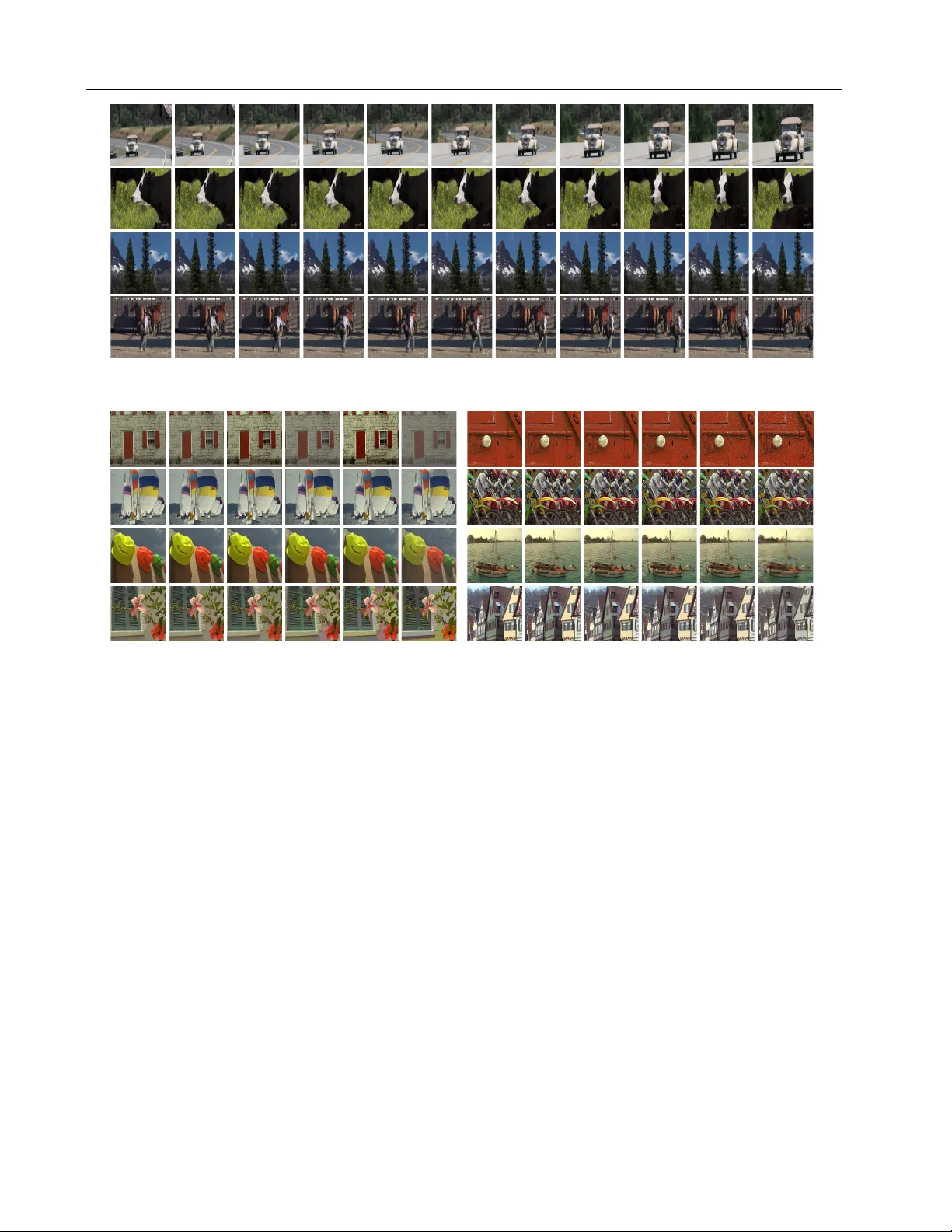
Learning Similarity Metrics f or Numerical Simulations Georg K ohl 1 Kiwon Um 1 Nils Thuerey 1 Abstract W e propose a neural network-based approach that computes a stable and generalizing metric ( LSiM ) to compare data from a variety of nu- merical simulation sources. W e focus on scalar time-dependent 2D data that commonly arises from motion and transport-based partial differen- tial equations (PDEs). Our method employs a Siamese network architecture that is motiv ated by the mathematical properties of a metric. W e le verage a controllable data generation setup with PDE solvers to create increasingly dif ferent out- puts from a reference simulation in a controlled en vironment. A central component of our learned metric is a specialized loss function that intro- duces knowledge about the correlation between single data samples into the training process. T o demonstrate that the proposed approach outper- forms existing metrics for vector spaces and other learned, image-based metrics, we ev aluate the dif- ferent methods on a lar ge range of test data. Addi- tionally , we analyze generalization beneﬁts of an adjustable training data dif ﬁculty and demonstrate the robustness of LSiM via an ev aluation on three real-world data sets. 1. Introduction Evaluating computational tasks for complex data sets is a fundamental problem in all computational disciplines. Reg- ular vector space metrics, such as the L 2 distance, were shown to be v ery unreliable ( W ang et al. , 2004 ; Zhang et al. , 2018 ), and the advent of deep learning techniques with con- volutional neural networks (CNNs) made it possible to more reliably ev aluate complex data domains such as natural im- ages, texts ( Benajiba et al. , 2018 ), or speech ( W ang et al. , 2018 ). Our central aim is to demonstrate the usefulness of 1 Department of Informatics, T echnical Univ ersity of Mu- nich, Munich, Germany . Correspondence to: Georg Kohl < georg.k ohl@tum.de > . Pr oceedings of the 37 th International Conference on Machine Learning , V ienna, Austria, PMLR 119, 2020. Copyright 2020 by the author(s). CNN-based ev aluations in the context of numerical simula- tions. These simulations are the basis for a wide range of applications ranging from blood ﬂow simulations to aircraft design. Speciﬁcally , we propose a nov el learned simulation metric ( LSiM ) that allo ws for a reliable similarity e valuation of simulation data. Potential applications of such a metric arise in all areas where numerical simulations are performed or similar data is gathered from observ ations. For example, accurate ev alua- tions of existing and ne w simulation methods with respect to a known ground truth solution ( Oberkampf et al. , 2004 ) can be performed more reliably than with a regular vector norm. Another good example is weather data for which comple x transport processes and chemical reactions make in-place comparisons with common metrics unreliable ( Jolliffe & Stephenson , 2012 ). Like wise, the long-standing, open ques- tions of turb ulence ( Moin & Mahesh , 1998 ; Lin et al. , 1998 ) can beneﬁt from improved methods for measuring the simi- larity and differences in data sets and observ ations. In this work, we focus on ﬁeld data, i.e., dense grids of scalar values, similar to images, which were generated with known partial differential equations (PDEs) in order to en- sure the av ailability of ground truth solutions. While we focus on 2D data in the following to mak e comparisons with existing techniques from imaging applications possible, our approach naturally extends to higher dimensions. Every sample of this 2D data can be regarded a high dimensional vector , so metrics on the corresponding vector space are applicable to ev aluate similarities. These metrics, in the following denoted as shallow metrics , are typically simple, element-wise functions such as L 1 or L 2 distances. Their inherent problem is that they cannot compare structures on different scales or conte xtual information. Many practical problems require solutions over time and need a vast number of non-linear operations that often re- sult in substantial changes of the solutions even for small changes of the inputs. Hence, despite being based on known, continuous formulations, these systems can be seen as chaotic . W e illustrate this behavior in Fig. 1 , where tw o smoke ﬂows are compared to a reference simulation. A single simulation parameter was v aried for these examples, and a visual inspection shows that smoke plume (a) is more similar to the reference. This matches the data generation Learning Similarity Metrics f or Numerical Simulations Figure 1. Example of ﬁeld data from a ﬂuid simulation of hot smoke with normalized distances for different metrics. Our method ( LSiM , green) approximates the ground truth distances (GT , gray) determined by the data generation method best, i.e., version (a) is closer to the ground truth data than (b). An L 2 metric (red) erroneously yields a rev ersed ordering. process: version (a) has a signiﬁcantly smaller parameter change than (b) as shown in the inset graph on the right. LSiM robustly predicts the ground truth distances while the L 2 metric labels plume (b) as more similar . In our work, we focus on retrie ving the relative distances of simulated data sets. Thus, we do not aim for retrieving the absolute param- eter change b ut a relati ve distance that preserves ordering with respect to this parameter . Using existing image metrics based on CNNs for this prob- lem is not optimal either: natural images only cov er a small fraction of the space of possible 2D data, and numerical simulation outputs are located in a fundamentally dif ferent data manifold within this space. Hence, there are crucial aspects that cannot be captured by purely learning from photographs. Furthermore, we have full control ov er the data generation process for simulation data. As a result, we can create arbitrary amounts of training data with gradual changes and a ground truth ordering. W ith this data, we can learn a metric that is not only able to directly e xtract and use features but also encodes interactions between them. The central contributions of our w ork are as follo ws: • W e propose a Siamese network architecture with fea- ture map normalization, which is able to learn a metric that generalizes well to unseen motion and transport- based simulation methods. • W e propose a novel loss function that combines a cor - relation loss term with a mean squared error to improv e the accuracy of the learned metric. • In addition, we sho w ho w a data generation approach for numerical simulations can be employed to train networks with general and robust feature e xtractors for metric calculations. Our source code, data sets, and ﬁnal model are a v ailable at https://github.com/tum- pbs/LSIM . 2. Related W ork One of the earliest methods to go beyond using simple met- rics based on L p norms for natural images was the structural similarity index ( W ang et al. , 2004 ). Despite improvements, this method can still be considered a shallow metric. Over the years, multiple large databases for human e v aluations of natural images were presented, for instance, CSIQ ( Larson & Chandler , 2010 ), TID2013 ( Ponomarenko et al. , 2015 ), and CID:IQ ( Liu et al. , 2014 ). W ith this data and the disco v- ery that CNNs can create v ery powerful feature e xtractors that are able to recognize patterns and structures, deep fea- ture maps quickly became established as means for e v alua- tion ( Amirshahi et al. , 2016 ; Berardino et al. , 2017 ; Bosse et al. , 2016 ; Kang et al. , 2014 ; Kim & Lee , 2017 ). Recently , these methods were improved by predicting the distribution of human e valuations instead of directly learning distance values ( Prashnani et al. , 2018 ; T alebi & Milanfar , 2018b ). Zhang et al. compared different architecture and lev els of supervision, and showed that metrics can be interpreted as a transfer learning approach by applying a linear weighting to the feature maps of any network architecture to form the image metric LPIPS v0.1 . T ypical use cases of these image- based CNN metrics are computer vision tasks such as detail enhancement ( T alebi & Milanfar , 2018a ), style transfer , and super-resolution ( Johnson et al. , 2016 ). Generativ e adver - sarial networks also le verage CNN-based losses by training a discriminator network in parallel to the generation task ( Dosovitskiy & Brox , 2016 ). Siamese network architectures are kno wn to work well for a variety of comparison tasks such as audio ( Zhang & Duan , 2017 ), satellite images ( He et al. , 2019 ), or the similarity of interior product designs ( Bell & Bala , 2015 ). Furthermore, they yield robust object trackers ( Bertinetto et al. , 2016 ), algorithms for image patch matching ( Hanif , 2019 ), and for descriptors for ﬂuid ﬂo w synthesis ( Chu & Thuerey , 2017 ). Inspired by these studies, we use a similar Siamese neural network architecture for our metric learning task. In contrast to other work on self-supervised learning that utilizes spatial or temporal changes to learn meaningful representations ( Agrawal et al. , 2015 ; W ang & Gupta , 2015 ), our method does not rely on tracked ke ypoints in the data. While correlation terms have been used for learning joint representations by maximizing correlation of projected Learning Similarity Metrics f or Numerical Simulations views ( Chandar et al. , 2016 ) and are popular for style trans- fer applications via the Gram matrix ( Ruder et al. , 2016 ), they were not used for learning distance metrics. As we demonstrate below , they can yield signiﬁcant improvements in terms of the inferred distances. Similarity metrics for numerical simulations are a topic of ongoing in vestigation. A variety of specialized metrics hav e been proposed to overcome the limitations of L p norms, such as the displacement and amplitude score from the area of weather forecasting ( K eil & Craig , 2009 ) as well as per - mutation based metrics for energy consumption forecasting ( Haben et al. , 2014 ). T urbulent ﬂo ws, on the other hand, are often e v aluated in terms of aggregated frequency spectra ( Pitsch , 2006 ). Crowd-sourced ev aluations based on the human visual system were also proposed to ev aluate simula- tion methods for physics-based animation ( Um et al. , 2017 ) and for comparing non-oscillatory discretization schemes ( Um et al. , 2019 ). These results indicate that visual e v alua- tions in the context of ﬁeld data are possible and robust, but they require extensi ve (and potentially expensi ve) user stud- ies. Additionally , our method naturally extends to higher dimensions, while human e valuations inherently rely on pro- jections with at most two spatial and one time dimension. 3. Constructing a CNN-based Metric In the following, we explain our considerations when em- ploying CNNs as e v aluation metrics. For a comparison that corresponds to our intuiti ve understanding of distances, an underlying metric has to obey certain criteria. More pre- cisely , a function m : I × I → [0 , ∞ ) is a metric on its input space I if it satisﬁes the follo wing properties ∀ x , y , z ∈ I : m ( x , y ) ≥ 0 non-negati vity (1) m ( x , y ) = m ( y , x ) symmetry (2) m ( x , y ) ≤ m ( x , z ) + m ( z , y ) triangle ineq. (3) m ( x , y ) = 0 ⇐ ⇒ x = y identity of indisc. (4) The properties ( 1 ) and ( 2 ) are crucial as distances should be symmetric and have a clear lower bound. Eq. ( 3 ) ensures that direct distances cannot be longer than a detour . Property ( 4 ), on the other hand, is not really useful for discrete opera- tions as approximation errors and ﬂoating point operations can easily lead to a distance of zero for slightly different inputs. Hence, we focus on a relaxed, more meaningful deﬁnition m ( x , x ) = 0 ∀ x ∈ I , which leads to a so-called pseudometric . It allows for a distance of zero for different inputs but has to be able to spot identical inputs. W e realize these requirements for a pseudometric with an architecture that follows popular perceptual metrics such as LPIPS : The activ ations of a CNN are compared in latent space, accumulated with a set of weights, and the resulting per-feature distances are aggregated to produce a ﬁnal dis- tance value. Fig. 2 giv es a visual overvie w of this process. T o sho w that the proposed Siamese architecture by construc- tion qualiﬁes as a pseudometric, the function m ( x , y ) = m 2 ( m 1 ( x ) , m 1 ( y )) computed by our network is split into two parts: m 1 : I → L to compute the latent space embeddings ˜ x = m 1 ( x ) , ˜ y = m 1 ( y ) from each input, and m 2 : L → [0 , ∞ ) to compare these points in the latent space L . W e chose operations for m 2 such that it forms a metric ∀ ˜ x , ˜ y ∈ L . Since m 1 always maps to L , this means m has the properties ( 1 ), ( 2 ), and ( 3 ) on I for any possible mapping m 1 , i.e., only a metric on L is required. T o achieve property ( 4 ), m 1 would need to be injecti ve, b ut the compression of typical feature extractors precludes this. Ho we ver , if m 1 is deterministic m ( x , x ) = 0 ∀ x ∈ I is still fulﬁlled since identical inputs result in the same point in latent space and thus a distance of zero. More details for this proof can be found in App. A . 3.1. Base Network The sole purpose of the base netw ork (Fig. 2 , in purple) is to extract feature maps from both inputs. The Siamese architec- ture implies that the weights of the base network are shared for both inputs, meaning all feature maps are comparable. W e e xperimented with the feature extracting layers from var - B a s e n e t w o r k I n p u t 1 I n p u t 2 B a s e n e t w o r k F e a tu r e m a p n o r m a liza tio n F e a tu r e m a p n o r m a liz a tio n E le m e n tw is e la te n t sp a c e d if fe r e n c e Ch a n n e l a g g r . : w e ig h t e d a v g . S p a ti a l a g g r .: a v e r a g e L a ye r a g g r .: su m m a tio n Dista n c e o u tp u t 1 L e a r n e d w e ig h t p e r fe a tu r e m a p R G B i n p u t s F e a t u r e ma p s: se t s o f 3 r d o r d e r t e n so r s D i f f e re n ce m a p s: se t o f 3 r d o r d e r t e n so rs A ve ra g e ma p s : se t o f 2 n d o r d e r t e n so r s L a ye r d i st a n ce s: se t o f sca l a r s d 1 d 2 d 3 d R e su l t : sca l a r Figure 2. Overvie w of the proposed distance computation for a simpliﬁed base network that contains three layers with four feature maps each in this example. The output shape for e very operation is illustrated below the transitions in orange and white. Bold operations are learned, i.e., contain weights inﬂuenced by the training process. Learning Similarity Metrics f or Numerical Simulations ious CNN architectures, such as AlexNet ( Krizhe vsky et al. , 2017 ), VGG ( Simon yan & Zisserman , 2015 ), SqueezeNet ( Iandola et al. , 2016 ), and a ﬂuid ﬂow prediction network ( Thuerey et al. , 2018 ). W e considered three variants of these networks: using the original pre-trained weights, ﬁne-tuning them, or re-training the full networks from scratch. In con- trast to typical CNN tasks where only the result of the ﬁnal output layer is further processed, we make use of the full range of extracted features across the layers of a CNN (see Fig. 2 ). This implies a slightly different goal compared to regular training: while early features should be general enough to allow for extracting more complex features in deeper layers, this is not their sole purpose. Rather , features in earlier layers of the network can directly participate in the ﬁnal distance calculation and can yield important cues. W e achiev ed the best performance for our data sets using a base network architecture with ﬁv e layers, similar to a re- duced AlexNet, that was trained from scratch (see App. B.1 ). This feature extractor is fully con volutional and thus allows for v arying spatial input dimensions, b ut for comparability to other models we keep the input size constant at 224 × 224 for our ev aluation. In separate tests with interpolated inputs, we found that the metric still works well for scaling factors in the range [0 . 5 , 2] . 3.2. Featur e Map Normalization The goal of normalizing the feature maps (Fig. 2 , in red) is to transform the extracted features of each layer , which typi- cally hav e very dif ferent orders of magnitude, into compara- ble ranges. While this task could potentially be performed by the learned weights, we found the normalization to yield improv ed performance in general. Let G denote a 4 th order feature tensor with dimensions ( g b , g c , g x , g y ) from one layer of the base netw ork. W e form a series G 0 , G 1 , . . . for ev ery possible content of this tensor across our training samples. The normalization only hap- pens in the channel dimension, so all follo wing operations accumulate values along the dimension of g c while keeping g b , g x , and g y constant, i.e., are applied independently of the batch and spatial dimensions. The unit length normalization proposed by Zhang et al. , i.e., norm unit ( G ) = G / k G k 2 , only considers the current sample. In this case, k G k 2 is a 3 rd order tensor with the Euclidean norms of G along the channel dimension. Effecti vely , this results in a cosine distance, which only measures angles of the latent space vectors. T o consider the vector magnitude, the most basic idea is to use the maximum norm of other training samples, and this leads to a global unit length normalization norm global ( G ) = G / max ( k G 0 k 2 , k G 1 k 2 , . . . ) . Now , the magnitude of the current sample can be compared to other feature vectors, but this is not robust since the largest feature vector could be an outlier with respect to the typical content. Instead, we individually transform each component of a feature vector with dimension g c to a standard normal distribution. This is realized by subtracting the mean and dividing by the standard deviation of all features element- wise along the channel dimension as follows: norm dist ( G ) = 1 √ g c − 1 G − mean ( G 0 , G 1 , . . . ) std ( G 0 , G 1 , . . . ) . These statistics are computed via a preprocessing step over the training data and stay ﬁx ed during training, as we did not observe signiﬁcant improv ements with more complicated schedules such as keeping a running mean. The magnitude of the resulting normalized vectors follo ws a chi distribution with k = g c degrees of freedom, but computing its mean √ 2 Γ(( k + 1) / 2) / Γ( k / 2) is expensi ve 1 , especially for larger k . Instead, the mode of the chi distribution √ g c − 1 that closely approximates its mean is employed to achie ve a consistent a verage magnitude of about one independently of g c . As a result, we can measure angles for the latent space vectors and compare their magnitude in the global length distribution across all layers. 3.3. Latent Space Differences Computing the difference of two latent space representations ˜ x , ˜ y ∈ L that consist of all extracted features from the tw o inputs x , y ∈ I lies at the core of the metric. This dif ference operator in combination with the following aggregations has to ensure that the metric properties above are upheld with respect to L . Thus, the most obvious approach to employ an element-wise dif ference ˜ x i − ˜ y i ∀ i ∈ { 0 , 1 , . . . , dim ( L ) } is not suitable, as it in validates non-ne gati vity and symmetry . Instead, exponentiation of an absolute dif ference via | ˜ x i − ˜ y i | p yields an L p metric on L , when combined with the correct aggregation and a p th root. | ˜ x i − ˜ y i | 2 is used to compute the dif ference maps (Fig. 2 , in yello w), as we did not observe signiﬁcant dif ferences for other values of p . Considering the importance of comparing the extracted fea- tures, this simple feature dif ference does not seem optimal. Rather , one can imagine that improvements in terms of com- paring one set of feature activ ations could lead to ov erall improv ements for deri ved metrics. W e in vestigated replac- ing these operations with a pre-trained CNN-based metric for each feature map. This creates a recursiv e process or “meta-metric” that reformulates the initial problem of learn- ing input similarities in terms of learning feature space sim- ilarities. Howev er, as detailed in App. B.3 , we did not ﬁnd any substantial impro vements with this recursi ve approach. This implies that once a large enough number of expressi ve 1 Γ denotes the gamma function for factorials Learning Similarity Metrics f or Numerical Simulations features is av ailable for comparison, the in-place difference of each feature is sufﬁcient to compare tw o inputs. 3.4. Aggregations The subsequent aggre gation operations (Fig. 2 , in green) are applied to the difference maps to compress the contained per feature differences along the dif ferent dimensions into a single distance value. A simple summation in combination with an absolute dif ference | ˜ x i − ˜ y i | abov e leads to an L 1 distance on the latent space L . Similarly , we can show that av erage or learned weighted av erage operations are applica- ble too (see App. A ). In addition, using a p -th power for the latent space difference requires a corresponding root opera- tion after all aggregations, to ensure the metric properties with respect to L . T o aggregate the dif ference maps along the channel dimen- sion, we found the weighted average proposed by Zhang et al. to work very well. Thus, we use one learnable weight to control the importance of a feature. The weight is a multiplier for the corresponding difference map before sum- mation along the channel dimension, and is clamped to be non-negati ve. A negati ve weight w ould mean that a lar ger difference in this feature produces a smaller ov erall distance, which is not helpful. F or regularization, the learned ag- gregation weights utilize dropout during training, i.e., are randomly set to zero with a probability of 50%. This ensures that the network cannot rely on single features only , but has to consider multiple features for a more stable ev aluation. For spatial and layer aggre gation, functions such as a sum- mation or av eraging are sufﬁcient and generally interchange- able. W e experimented with more intricate aggregation func- tions, e.g., by learning a spatial av erage or determining layer importance weights dynamically from the inputs. When the base network is ﬁx ed and the metric only has very fe w train- able weights, this did improve the o verall performance. But, with a fully trained base network, the feature e xtraction seems to automatically adopt these aspects making a more complicated aggregation unnecessary . 4. Data Generation and T raining Similarity data sets for natural images typically rely on changing already existing images with distortions, noise, or other operations and assigning ground truth distances according to the strength of the operation. Since we can control the data creation process for numerical simulations directly , we can generate lar ge amounts of simulation data with increasing dissimilarities by altering the parameters used for the simulations. As a result, the data contains more information about the nature of the problem, i.e., which changes of the data distribution should lead to increased distances, than by applying modiﬁcations as a post-process. 4.1. Data Generation Giv en a set of model equations, e.g., a PDE from ﬂuid dy- namics, typical solution methods consist of a solver that, giv en a set of boundary conditions, computes discrete ap- proximations of the necessary differential operators. The discretized operators and the boundary conditions typically contain problem dependent parameters, which we collec- tiv ely denote with p 0 , p 1 , . . . , p i , . . . in the following. W e only consider time dependent problems, and our solvers start with initial conditions at t 0 to compute a series of time steps t 1 , t 2 , . . . until a target point in time ( t t ) is reached. At that point, we obtain a reference output ﬁeld o 0 from one of the PDE variables, e.g., a v elocity . I n it i a l c o n d it i o n s O u t p u t F in i t e d if f e r e n c e s o lv e r w i t h t im e d i s c r e t i za t i o n [ p 0 p 1 ⋯ p i ] t 1 t 2 t t o 0 o 1 [ p 0 p 1 ⋯ p i + Δ i ] [ p 0 p 1 ⋯ p i + n ⋅ Δ i ] t 1 t 2 t t o n I n c r e a s i n g p a r a m e t e r c h a n g e D e c r e a s i n g o u t p u t s i m i l a r i t y n o ise 1 , 1 ( s ) n o ise 1 , 2 ( s ) n o ise 1 , t ( s ) t 1 t 2 t t n o ise 2 , 1 ( s ) n o ise 2 , 2 ( s ) n o ise 2 , t ( s ) n o ise n , 1 ( s ) n o ise n , 2 ( s ) n o ise n , t ( s ) Figure 3. General data generation method from a PDE solv er for a time dependent problem. With increasing changes of the initial conditions for a parameter p i in ∆ i increments, the outputs de- crease in similarity . Controlled Gaussian noise is injected in a simulation ﬁeld of the solver . The difﬁculty of the learning task can be controlled by scaling ∆ i as well as the noise variance v . For data generation, we incrementally change a single pa- rameter p i in n steps ∆ i , 2 · ∆ i , . . . , n · ∆ i to create a series of n outputs o 1 , o 2 , . . . , o n . W e consider a series obtained in this way to be increasingly different from o 0 . T o create natural variations of the resulting data distrib utions, we add Gaussian noise ﬁelds with zero mean and adjustable vari- ance v to an appropriate simulation ﬁeld such as a v elocity . This noise allows us to generate a large number of v aried data samples for a single simulation parameter p i . Further- more, v serves as an additional parameter that can be varied in isolation to observe the same simulation with different lev els of interference. This is similar in nature to numerical errors introduced by discretization schemes. These pertur- bations enlarge the space co vered by the training data, and we found that training networks with suitable noise le vels improv es robustness as we will demonstrate below . The process for data generation is summarized in Fig. 3 . As PDEs can model extremely complex and chaotic be- haviour , there is no guarantee that the outputs always ex- hibit increasing dissimilarity with the increasing parameter change. This behaviour is what makes the task of similar- Learning Similarity Metrics f or Numerical Simulations ity assessment so challenging. Even if the solutions are essentially chaotic, their behaviour is not arbitrary b ut rather gov erned by the rules of the underlying PDE. F or our data set, we choose the follo wing range of representati ve PDEs: W e include a pure Advection-Diffusion model (AD), and Burger’ s equation (BE) which introduces an additional vis- cosity term. Furthermore, we use the full Navier -Stokes equations (NSE), which introduce a conservation of mass constraint. When combined with a deterministic solver and a suitable parameter step size, all these PDEs exhibit chaotic behaviour at small scales, and the medium to large scale characteristics of the solutions shift smoothly with increas- ing changes of the parameters p i . The noise ampliﬁes the chaotic behaviour to larger scales and provides a controlled amount of perturbations for the data generation. This lets the network learn about the nature of the chaotic behaviour of PDEs without o verwhelming it with data where patterns are not observ able anymore. The latter can easily happen when ∆ i or v grow too large and produce essentially random outputs. Instead, we speciﬁcally target solutions that are dif ﬁcult to ev aluate in terms of a shallow metric. W e heuristically select the smallest v and a suitable ∆ i such that the ordering of several random output samples with respect to their L 2 difference drops below a correlation value of 0 . 8 . For the chosen PDEs, v was small enough to av oid deterioration of the physical behaviour especially due to the diffusion terms, but dif ferent means of adjusting the difﬁculty may be necessary for other data. 4.2. T raining For training, the 2D scalar ﬁelds from the simulations were augmented with random ﬂips, 90 ◦ rotations, and cropping to obtain an input size of 224 × 224 ev ery time they are used. Identical augmentations were applied to each ﬁeld of one given sequence to ensure comparability . Afterwards, each input sequence is collectiv ely normalized to the range [0 , 255] . T o allo w for comparisons with image metrics and provide the possibility to compare color data and full ve- locity ﬁelds during inference, the metric uses three input channels. During training, the scalar ﬁelds are duplicated to each channel after augmentation. Unless otherwise noted, networks were trained with a batch size of 1 for 40 epochs with the Adam optimizer using a learning rate of 10 − 5 . T o ev aluate the trained networks on v alidation and test inputs, only a bilinear resizing and the normalization step is applied. 5. Correlation Loss Function The central goal of our networks is to identify relati ve dif- ferences of input pairs produced via numerical simulations. Thus, instead of employing a loss that forces the network to only infer giv en labels or distance v alues, we train our networks to infer the ordering of a given sequence of simula- tion outputs o 0 , o 1 , . . . , o n . W e propose to use the Pearson correlation coefﬁcient (see Pearson , 1920 ), which yields a value in [ − 1 , 1] that measures the linear relationship be- tween two distrib utions. A value of 1 implies that a linear equation describes their relationship perfectly . W e com- pute this coefﬁcient for a full series of outputs such that the network can learn to extract features that arrange this data series in the correct ordering. Each training sample of our network consists of e very possible pair from the sequence o 0 , o 1 , . . . , o n and the corresponding ground truth distance distribution c ∈ [0 , 1] 0 . 5( n +1) n representing the parameter change from the data generation. For a distance prediction d ∈ [0 , ∞ ) 0 . 5( n +1) n of our network for one sample, we compute the loss with: L ( c , d ) = λ 1 ( c − d ) 2 + λ 2 (1 − ( c − ¯ c ) · ( d − ¯ d ) k c − ¯ c k 2   d − ¯ d   2 ) (5) Here, the mean of a distance vector is denoted by ¯ c and ¯ d for ground truth and prediction, respectiv ely . The ﬁrst part of the loss is a regular MSE term, which minimizes the difference between predicted and actual distances. The second part is the Pearson correlation coef ﬁcient, which is in verted such that the optimization results in a maximization of the correlation. As this formulation depends on the length of the input sequence, the two terms are scaled to adjust their relativ e inﬂuence with λ 1 and λ 2 . For the training, we chose n = 10 variations for each reference simulation. If n should vary during training, the inﬂuence of both terms needs to be adjusted accordingly . W e found that scaling both terms to a similar order of magnitude worked best in our experiments.                        L S i M ( o u r s ) A l e x N e t f r o z e n Figure 4. Performance comparison on our test data of the proposed approach ( LSiM ) and a smaller model ( Ale xNet fr ozen ) for different loss functions on the y-axis. In Fig. 4 , we in vestigate how the proposed loss function compares to other commonly used loss formulations for our full network and a pre-trained network, where only aggre- gation weights are learned. The performance is measured via Spearman’ s rank correlation of predicted against ground truth distances on our combined test data sets. This is com- parable to the All column in T ab . 1 and described in more Learning Similarity Metrics f or Numerical Simulations detail in Section 6.2 . In addition to our full loss function, we consider a loss function that replaces the Pearson correlation with a simpler cross-correlation ( c · d ) / ( k c k 2 k d k 2 ) . W e also include networks trained with only the MSE or only the correlation terms for each of the two v ariants. A simple MSE loss yields the worst performance for both ev aluated models. Using any correlation based loss function for the AlexNet fr ozen metric (see Section 6.2 ) improves the results, but there is no major difference due to the limited number of only 1152 trainable weights. For LSiM , the pro- posed combination of MSE loss with the Pearson correlation performs better than using cross-correlation or only isolated Pearson correlation. Interestingly , combining cross correla- tion with MSE yields worse results than cross correlation by itself. This is caused by the cross correlation term inﬂu- encing absolute distance values, which potentially conﬂicts with the MSE term. For our loss, the Pearson correlation only handles the relati ve ordering while the MSE deals with the absolute distances, leading to better inferred distances. 6. Results In the following, we will discuss how the data generation approach was emplo yed to create a lar ge range of training and test data from different PDEs. Afterwards, the proposed metric is compared to other metrics, and its robustness is ev aluated with sev eral external data sets. 6.1. Data Sets W e created four training ( Smo , Liq , Adv and Bur ) and two test data sets ( LiqN and AdvD ) with ten parameter steps for each reference simulation. Based on two 2D NSE solvers, the smoke and liquid simulation training sets ( Smo and Liq ) add noise to the velocity ﬁeld and feature varied initial conditions such as ﬂuid position or obstacle properties, in addition to v ariations of b uoyancy and gra vity forces. The two other training sets ( Adv and Bur ) are based on 1D solvers for AD and BE, concatenated over time to form a 2D result. In both cases, noise w as injected into the v elocity ﬁeld, and the v aried parameters are changes to the ﬁeld initialization and forcing functions. For the test data set, we substantially change the data dis- tribution by injecting noise into the density instead of the velocity ﬁeld for AD simulations to obtain the AdvD data set and by including background noise for the velocity ﬁeld of a liquid simulation ( LiqN ). In addition, we employed three more test sets ( Sha , Vid , and TID ) created without PDE models to explore the generalization for data far from our training data setup. W e include a shape data set ( Sha ) that features multiple randomized moving rigid shapes, a video data set ( Vid ) consisting of frames from random video footage, and TID2013 ( Ponomarenko et al. , 2015 ) as a perceptual image data set ( TID ). Belo w , we additionally list a combined correlation score ( All ) for all test sets apart from TID , which is e xcluded due to its different structure. Examples for each data set are sho wn in Fig. 5 and genera- tion details with further samples can be found in App. D . 6.2. Perf ormance Evaluation T o ev aluate the performance of a metric on a data set, we ﬁrst compute the distances from each reference simulation to all corresponding v ariations. Then, the predicted and the ground truth distance distributions o ver all samples are combined and compared using Spearman’ s rank correlation coefﬁcient (see Spearman , 1904 ). It is similar to the Pear- son correlation, but instead it uses ranking v ariables, i.e., measures monotonic relationships of distributions. The top part of T ab . 1 shows the performance of the shallo w metrics L 2 and SSIM as well as the LPIPS metric ( Zhang et al. , 2018 ) for all our data sets. The results clearly show that shallo w metrics are not suitable to compare the samples in our data set and only rarely achiev e good correlation values. The perceptual LPIPS metric performs better in general and outperforms our method on the image data sets Vid and TID . This is not surprising as LPIPS is speciﬁcally trained for such images. For most of the simulation data sets, howe ver , it performs signiﬁcantly worse than for the image content. The last row of T ab . 1 sho ws the results of our LSiM model with a very good performance across all data sets and no negati ve outliers. Note that although it was not trained with any natural image content, it still performs well for the image test sets. Figure 5. Samples from our data sets. For each subset the reference is on the left, and three v ariations in equal parameter steps follow . From left to right and top to bottom: Smo (density , velocity , and pressure), Adv (density), Liq (ﬂags, velocity , and lev elset), Bur (velocity), LiqN (velocity), AdvD (density), Sha and Vid . Learning Similarity Metrics f or Numerical Simulations T able 1. Performance comparison of existing metrics (top block), experimental designs (middle block), and variants of the proposed method (bottom block) on validation and test data sets measured in terms of Spearman’ s rank correlation coefﬁcient of ground truth against predicted distances. Bold+underlined values show the best performing metric for each data set, bold values are within a 0 . 01 error margin of the best performing, and italic values are 0 . 2 or more below the best performing. On the right, a visualization of the combined test data results is shown for selected models. Metric V alidation data sets T est data sets Smo Liq Adv Bur TID LiqN AdvD Sha Vid All L 2 0.66 0.80 0.74 0.62 0.82 0.73 0.57 0.58 0.79 0.61 SSIM 0.69 0.73 0.77 0.71 0.77 0.26 0.69 0.46 0.75 0.53 LPIPS v0.1. 0.63 0.68 0.68 0.72 0.86 0.50 0.62 0.84 0.83 0.66 AlexNet random 0.63 0.69 0.69 0.66 0.82 0.64 0.65 0.67 0.81 0.65 AlexNet fr ozen 0.66 0.70 0.69 0.71 0.85 0.40 0.62 0.87 0.84 0.65 Optical ﬂow 0.62 0.57 0.36 0.37 0.55 0.49 0.28 0.61 0.75 0.48 Non-Siamese 0.77 0.85 0.78 0.74 0.65 0.81 0.64 0.25 0.80 0.60 Skip fr om scratc h 0.79 0.83 0.80 0.74 0.85 0.78 0.61 0.78 0.83 0.71 LSiM noiseless 0.77 0.77 0.76 0.72 0.85 0.62 0.58 0.86 0.82 0.68 LSiM str ong noise 0.65 0.65 0.67 0.69 0.84 0.39 0.54 0.89 0.82 0.64 LSiM (ours) 0.78 0.82 0.79 0.75 0.86 0.79 0.58 0.88 0.81 0.73 L 2 S S I M L P I P S O p t F l o w N o n S i a m S k i p L S i M          The middle block of T ab . 1 contains several interesting v ari- ants (more details can be found in App. B ): AlexNet random and AlexNet fr ozen are small models, where the base net- work is the original AlexNet with pre-trained weights. AlexNet random contains purely random aggreg ation weights without training, whereas AlexNet fr ozen only has trainable weights for the channel aggregation and therefore lacks the ﬂexibility to fully adjust to the data distribution of the numerical simulations. The random model performs surpris- ingly well in general, pointing to po wers of the underlying Siamese CNN architecture. Recognizing that many PDEs include transport phenomena, we in vestigated optical ﬂo w ( Horn & Schunck , 1981 ) as a means to compute motion from ﬁeld data. For the Optical ﬂow metric, we used Flo wNet2 ( Ilg et al. , 2016 ) to bidirec- tionally compute the optical ﬂo w ﬁeld between two inputs and aggregate it to a single distance v alue by summing all ﬂow v ector magnitudes. On the data set Vid that is similar to the training data of FlowNet2, it performs relativ ely well, but in most other cases it performs poorly . This sho ws that computing a simple warping from one input to the other is not enough for a stable metric although it seems lik e an in- tuitiv e solution. A more rob ust metric needs the knowledge of the underlying features and their changes to generalize better to new data. T o ev aluate whether a Siamese architecture is really ben- eﬁcial, we used a Non-Siamese architecture that directly predicts the distance from both stacked inputs. F or this purpose, we employed a modiﬁed version of Ale xNet that reduces the weights of the feature extractor by 50% and of the remaining layers by 90%. As expected, this metric works great on the validation data but has huge problems with generalization, especially on TID and Sha . In addi- tion, e ven simple metric properties such as symmetry are no longer guaranteed because this architecture does not hav e the inherent constraints of the Siamese setup. Finally , we experimented with multiple fully trained base networks. As re-training existing feature extractors only provided small improv ements, we used a custom base network with skip connections for the Skip fr om scratc h metric. Its results already come close to the proposed approach on most data sets. The last block in T ab . 1 shows variants of the proposed approach trained with varied noise lev els. This inherently changes the dif ﬁculty of the data. Hence, LSiM noiseless was trained with relatively simple data without perturbations, whereas LSiM str ong noise was trained with strongly varying data. Both cases decrease the capabilities of the trained model on some of the v alidation and test sets. This indicates that the network needs to see a certain amount of v ariation at training time in order to become rob ust, but o verly large changes hinder the learning of useful features (also see App. C ). 6.3. Evaluation on Real-W orld Data T o ev aluate the generalizing capabilities of our trained met- ric, we turn to three representati ve and publicly av ailable data sets of captured and simulated real-world phenomena, namely buoyant ﬂows, turbulence, and weather . For the former , we make use of the ScalarFlow data set ( Eckert et al. , 2019 ), which consists of captured velocities of buo y- ant scalar transport ﬂows. Additionally , we include velocity data from the Johns Hopkins T urbulence Database ( JHTDB ) Learning Similarity Metrics f or Numerical Simulations Figure 6. Examples from three real-world data repositories used for ev aluation, visualized via color-mapping. Each block features four different sequences (rows) with frames in equal temporal or spatial intervals. Left: ScalarFlow – captured buo yant volumetric transport ﬂows using the z-slice (top tw o) and z-mean (bottom two). Middle: JHTDB – four different turb ulent DNS simulations. Right: W eatherBench – weather data consisting of temperature (top two) and geopotential (bottom two). ( Perlman et al. , 2007 ), which represents direct numerical simulations of fully de veloped turbulence. As a third case, we use scalar temperature and geopotential ﬁelds from the W eatherBench repository ( Rasp et al. , 2020 ), which contains global climate data on a Cartesian latitude-longitude grid of the earth. V isualizations of this data via color-mapping the scalar ﬁelds or velocity magnitudes are sho wn in Fig. 6 . L 2 S S I M L P I P S L S i M ( o u r s )       S c a l a r F l o w J H T D B W e a t h e r B e n c h Figure 7. Spearman correlation values for multiple metrics on data from three repositories. Shown are mean and standard deviation ov er different temporal or spatial interv als used to create sequences. For the results in Fig. 7 , we extracted sequences of frames with ﬁxed temporal and spatial interv als from each data set to obtain a ground truth ordering. Six different interval spac- ings for ev ery data source are employed, and all velocity data is split by component. W e then measure ho w well dif- ferent metrics recov er the original ordering in the presence of the comple x changes of content, dri ven by the underlying physical processes. The LSiM model outlined in previous sections was used for inference without further changes. Every metric is separately ev aluated (see Section 6.2 ) for the six interval spacings with 180-240 sequences each. For ScalarFlow and W eatherBench , the data was additionally partitioned by z-slice or z-mean and temperature or geopo- tential respecti vely , leading to twelve e v aluations. Fig. 7 shows the mean and standard de viation of the resulting cor- relation values. Despite nev er being trained on any data from these data sets, LSiM recov ers the ordering of all three cases with consistently high accuracy . It yields averaged correlations of 0 . 96 ± 0 . 02 , 0 . 95 ± 0 . 05 , and 0 . 95 ± 0 . 06 for ScalarFlow , JHTDB , and W eatherBench , respecti vely . The other metrics show lo wer means and higher uncertainty . Further details and results for the individual e valuations can be found in App. E . 7. Conclusion W e have presented the LSiM metric to reliably and robustly compare outputs from numerical simulations. Our method signiﬁcantly outperforms existing shallo w metric functions and provides better results than other learned metrics. W e demonstrated the usefulness of the correlation loss, showed the beneﬁts of a controlled data generation environment, and highlighted the stability of the obtained metric for a range of real-world data sets. Our trained LSiM metric has the potential to impact a wide range of ﬁelds, including the f ast and reliable accuracy as- sessment of new simulation methods, robust optimizations of parameters for reconstructions of observations, and guid- ing generativ e models of physical systems. Furthermore, it will be highly interesting to e v aluate other loss functions, e.g., mutual information ( Bachman et al. , 2019 ) or con- trastiv e predictive coding ( H ´ enaff et al. , 2019 ), and combi- nations with ev aluations from perceptual studies ( Um et al. , 2019 ). W e also plan to ev aluate our approach for an ev en larger set of PDEs as well as for 3D and 4D data sets. Espe- cially , turb ulent ﬂo ws are a highly relev ant and interesting area for future work on learned e valuation metrics. Learning Similarity Metrics f or Numerical Simulations Acknowledgements This work was supported by the ERC Starting Grant r e- alFlow (StG-2015-637014). W e would like to thank Stephan Rasp for preparing the W eatherBench data and all revie wers for helping to improv e this work. References Agrawal, P ., Carreira, J., and Malik, J. Learning to see by moving. In 2015 IEEE International Conference on Computer V ision (ICCV) , pp. 37–45, 2015. doi: 10.1109/ICCV .2015.13 . Amirshahi, S. A., Pedersen, M., and Y u, S. X. Image Qual- ity Assessment by Comparing CNN Features between Im- ages. Journal of Imaging Sience and T echnolo gy , 60(6), 2016. doi: 10.2352/J.ImagingSci.T echnol.2016.60.6.060410 . Bachman, P ., Hjelm, R. D., and Buchwalter, W . Learning rep- resentations by maximizing mutual information across views. CoRR , abs/1906.00910, 2019. URL abs/1906.00910 . Bell, S. and Bala, K. Learning visual similarity for product design with con volutional neural networks. ACM T ransactions on Graphics , 34(4):98:1–98:10, 2015. doi: 10.1145/2766959 . Benajiba, Y ., Sun, J., Zhang, Y ., Jiang, L., W eng, Z., and Biran, O. Siamese networks for semantic pattern similarity . CoRR , abs/1812.06604, 2018. URL 1812.06604 . Berardino, A., Balle, J., Laparra, V ., and Simoncelli, E. Eigen- Distortions of Hierarchical Representations. In Advances in Neu- ral Information Pr ocessing Systems 30 (NIPS 2017) , volume 30, 2017. URL . Bertinetto, L., V almadre, J., Henriques, J. F ., V edaldi, A., and T orr, P . H. S. Fully-Con volutional Siamese Networks for Object T racking. In Computer V ision - ECCV 2016 W orkshops, PT II , volume 9914, pp. 850–865, 2016. doi: 10.1007/978-3-319- 48881-3 56 . Bosse, S., Maniry , D., Mueller , K.-R., W iegand, T ., and Samek, W . Neural Network-Based Full-Reference Image Quality As- sessment. In 2016 Picture Coding Symposium (PCS) , 2016. doi: 10.1109/PCS.2016.7906376 . Chandar , S., Khapra, M. M., Larochelle, H., and Ravindran, B. Correlational neural networks. Neural Computation , 28(2): 257–285, 2016. doi: 10.1162/NECO a 00801 . Chu, M. and Thuerey , N. Data-Driv en Synthesis of Smoke Flows with CNN-based Feature Descriptors. ACM T ransactions on Gr aphics , 36(4):69:1–69:14, 2017. doi: 10.1145/3072959.3073643 . Dosovitskiy , A. and Brox, T . Generating Images with Percep- tual Similarity Metrics based on Deep Networks. In Advances in Neural Information Pr ocessing Systems 29 (NIPS 2016) , volume 29, 2016. URL 02644 . Eckert, M.-L., Um, K., and Thuerey , N. Scalarﬂow: A large- scale volumetric data set of real-w orld scalar transport ﬂo ws for computer animation and machine learning. ACM T ransactions on Graphics , 38(6), 2019. doi: 10.1145/3355089.3356545 . Goodfellow , I., Bengio, Y ., and Courville, A. Deep Learning . MIT Press, 2016. URL http://www.deeplearningbook. org . Haben, S., W ard, J., Greetham, D. V ., Singleton, C., and Grindrod, P . A new error measure for forecasts of household- lev el, high resolution electrical energy consumption. In- ternational Journal of F or ecasting , 30(2):246–256, 2014. doi: 10.1016/j.ijforecast.2013.08.002 . Hanif, M. S. Patch match networks: Improv ed tw o- channel and Siamese networks for image patch match- ing. P attern Recognition Letters , 120:54–61, 2019. doi: 10.1016/j.patrec.2019.01.005 . He, H., Chen, M., Chen, T ., Li, D., and Cheng, P . Learning to match multitemporal optical satellite images using multi- support-patches Siamese networks. Remote Sensing Letters , 10 (6):516–525, 2019. doi: 10.1080/2150704X.2019.1577572 . He, K., Zhang, X., Ren, S., and Sun, J. Deep residual learning for image recognition. In 2016 IEEE Conference on Computer V ision and P attern Recognition (CVPR) , pp. 770–778, 2016. doi: 10.1109/CVPR.2016.90 . H ´ enaff, O. J., Razavi, A., Doersch, C., Eslami, S. M. A., and van den Oord, A. Data-efﬁ cient image recognition with con- trastiv e predictive coding. CoRR , abs/1905.09272, 2019. URL http://arxiv.org/abs/1905.09272 . Horn, B. K. and Schunck, B. G. Determining optical ﬂow . Arti- ﬁcial intelligence , 17(1-3):185–203, 1981. doi: 10.1016/0004- 3702(81)90024-2 . Huang, G., Liu, Z., V an Der Maaten, L., and W einberger , K. Q. Densely connected con volutional netw orks. In 2017 IEEE Con- fer ence on Computer V ision and P attern Recognition (CVPR) , pp. 2261–2269, 2017. doi: 10.1109/CVPR.2017.243 . Iandola, F . N., Moskewicz, M. W ., Ashraf, K., Han, S., Dally , W . J., and Keutzer , K. Squeezenet: Alexnet-le vel accuracy with 50x fewer parameters and < 1mb model size. CoRR , abs/1602.07360, 2016. URL 1602.07360 . Ilg, E., Mayer, N., Saikia, T ., Keuper , M., Dosovitskiy , A., and Brox, T . Flownet 2.0: Evolution of optical ﬂo w estimation with deep networks. CoRR , abs/1612.01925, 2016. URL http: //arxiv.org/abs/1612.01925 . Johnson, J., Alahi, A., and Fei-Fei, L. Perceptual Losses for Real-T ime Style T ransfer and Super-Resolution. In Computer V ision - ECCV 2016, PT II , volume 9906, pp. 694–711, 2016. doi: 10.1007/978-3-319-46475-6 43 . Jolliffe, I. T . and Stephenson, D. B. F orecast veriﬁcation: a practitioner’ s guide in atmospheric science . John Wile y & Sons, 2012. doi: 10.1002/9781119960003 . Kang, L., Y e, P ., Li, Y ., and Doermann, D. Conv olutional Neural Networks for No-Reference Image Quality Assessment. In 2014 IEEE Confer ence on Computer V ision and P attern Recognition (CVPR) , pp. 1733–1740, 2014. doi: 10.1109/CVPR.2014.224 . Keil, C. and Craig, G. C. A displacement and amplitude score employing an optical ﬂow technique. W eather and F or ecasting , 24(5):1297–1308, 2009. doi: 10.1175/2009W AF2222247.1 . Learning Similarity Metrics f or Numerical Simulations Kim, J. and Lee, S. Deep Learning of Human V isual Sensitivity in Image Quality Assessment Framew ork. In 30TH IEEE Con- fer ence on Computer V ision and P attern Recognition (CVPR 2017) , pp. 1969–1977, 2017. doi: 10.1109/CVPR.2017.213 . Krizhevsk y , A., Sutskever , I., and Hinton, G. E. Imagenet classiﬁca- tion with deep conv olutional neural networks. Communications of the A CM , 60(6):84–90, 2017. doi: 10.1145/3065386 . Larson, E. C. and Chandler , D. M. Most apparent distor- tion: full-reference image quality assessment and the role of strategy . J ournal of Electr onic Imaging , 19(1), 2010. doi: 10.1117/1.3267105 . Lin, Z., Hahm, T . S., Lee, W ., T ang, W . M., and White, R. B. T urbulent transport reduction by zonal ﬂo ws: Massively parallel simulations. Science , 281(5384):1835–1837, 1998. doi: 10.1126/science.281.5384.1835 . Liu, X., Pedersen, M., and Hardeberg, J. Y . CID:IQ - A Ne w Image Quality Database. In Image and Signal Pr ocessing, ICISP 2014 , volume 8509, pp. 193–202, 2014. doi: 10.1007/978-3- 319-07998-1 22 . Moin, P . and Mahesh, K. Direct numerical simulation: a tool in turbulence research. Annual re view of ﬂuid mechanics , 30(1): 539–578, 1998. doi: 10.1146/annurev .ﬂuid.30.1.539 . Oberkampf, W . L., T rucano, T . G., and Hirsch, C. V eriﬁcation, v al- idation, and predictiv e capability in computational engineering and physics. Applied Mechanics Reviews , 57:345–384, 2004. doi: 10.1115/1.1767847 . Pearson, K. Notes on the History of Correlation. Biometrika , 13 (1):25–45, 1920. doi: 10.1093/biomet/13.1.25 . Perlman, E., Burns, R., Li, Y ., and Menev eau, C. Data exploration of turbulence simulations using a database cluster . In SC ’07: Pr oceedings of the 2007 ACM/IEEE Confer ence on Super com- puting , pp. 1–11, 2007. doi: 10.1145/1362622.1362654 . Pitsch, H. Large-eddy simulation of turbulent combus- tion. Annu. Rev . Fluid Mech. , 38:453–482, 2006. doi: 10.1146/annurev .ﬂuid.38.050304.092133 . Ponomarenko, N., Jin, L., Ieremeiev , O., Lukin, V ., Egiazarian, K., Astola, J., V ozel, B., Chehdi, K., Carli, M., Battisti, F ., and Kuo, C. C. J. Image database TID2013: Peculiarities, results and perspectiv es. Signal Pr ocessing-Image Communication , 30: 57–77, 2015. doi: 10.1016/j.image.2014.10.009 . Prashnani, E., Cai, H., Mostoﬁ, Y ., and Sen, P . Pieapp: Perceptual image-error assessment through pairwise preference. CoRR , abs/1806.02067, 2018. URL 1806.02067 . Rasp, S., Dueben, P ., Scher, S., W eyn, J., Mouatadid, S., and Thuerey , N. W eatherbench: A benchmark dataset for data- driv en weather forecasting. CoRR , abs/2002.00469, 2020. URL http://arxiv.org/abs/2002.00469 . Ronneberger , O., Fischer , P ., and Brox, T . U-net: Con volu- tional networks for biomedical image segmentation. CoRR , abs/1505.04597, 2015. URL 1505.04597 . Ruder , M., Dosovitskiy , A., and Brox, T . Artistic style trans- fer for videos. In P attern Recognition , pp. 26–36, 2016. doi: 10.1007/978-3-319-45886-1 3 . Simonyan, K. and Zisserman, A. V ery deep con volutional netw orks for large-scale image recognition. In ICLR , 2015. URL http: //arxiv.org/abs/1409.1556 . Spearman, C. The proof and measurement of association between two things. The American J ournal of Psychology , 15(1):72–101, 1904. doi: 10.2307/1412159 . T alebi, H. and Milanfar , P . Learned Perceptual Im- age Enhancement. In 2018 IEEE International Con- fer ence on Computational Photography (ICCP) , 2018a. doi: 10.1109/ICCPHO T .2018.8368474 . T alebi, H. and Milanfar, P . NIMA: Neural Image Assessment. IEEE T ransactions on Imag e Pr ocessing , 27(8):3998–4011, 2018b. doi: 10.1109/TIP .2018.2831899 . Thuerey , N., W eissenow , K., Mehrotra, H., Mainali, N., Prantl, L., and Hu, X. W ell, ho w accurate is it? A study of deep learn- ing methods for reynolds-a veraged navier -stokes simulations. CoRR , abs/1810.08217, 2018. URL abs/1810.08217 . Um, K., Hu, X., and Thuerey , N. Perceptual Evaluation of Liquid Simulation Methods. ACM T ransactions on Graphics , 36(4), 2017. doi: 10.1145/3072959.3073633 . Um, K., Hu, X., W ang, B., and Thuerey , N. Spot the Differ- ence: Accuracy of Numerical Simulations via the Human V isual System. CoRR , abs/1907.04179, 2019. URL http: //arxiv.org/abs/1907.04179 . W ang, X. and Gupta, A. Unsupervised learning of visual rep- resentations using videos. In 2015 IEEE International Con- fer ence on Computer V ision (ICCV) , pp. 2794–2802, 2015. doi: 10.1109/ICCV .2015.320 . W ang, Z., Bovik, A. C., Sheikh, H. R., and Simoncelli, E. Image quality assessment: From error visibility to structural similarity. IEEE T ransactions on Image Pr ocessing , 13(4):600–612, 2004. doi: 10.1109/TIP .2003.819861 . W ang, Z., Zhang, J., and Xie, Y . L2 Mispronunciation V eriﬁca- tion Based on Acoustic Phone Embedding and Siamese Net- works. In 2018 11TH International Symposium on Chinese Spoken Language Pr ocessing (ISCSLP) , pp. 444–448, 2018. doi: 10.1109/ISCSLP .2018.8706597 . Zhang, R., Isola, P ., Efros, A. A., Shechtman, E., and W ang, O. The Unreasonable Effecti veness of Deep Features as a Perceptual Metric. In 2018 IEEE Conference on Computer V ision and P attern Recognition (CVPR) , pp. 586–595, 2018. doi: 10.1109/CVPR.2018.00068 . Zhang, Y . and Duan, Z. IMINET : Con volutional Semi- Siamese Networks for Sound Search by V ocal Imita- tion. In 2017 IEEE W orkshop on Applications of Sig- nal Processing to Audio and Acoustics , pp. 304–308, 2017. doi: 10.1109/T ASLP .2018.2868428 . Zhu, Y . and Bridson, R. Animating sand as a ﬂuid. In ACM SIGGRAPH 2005 P apers , pp. 965–972, Ne w Y ork, NY , USA, 2005. doi: 10.1145/1186822.1073298 . A ppendix: Learning Similarity Metrics f or Numerical Simulations This supplemental document contains an analysis of the proposed metric design with respect to properties of metrics in general (App. A ) and details to the used network archi- tectures (App. B ). Afterwards, material that deals with the data sets is provided. It contains examples and failure cases for each of the data domains and analyzes the impact of the data dif ﬁculty (App. C and D ). Ne xt, the ev aluation on real-world data is described in more detail (App. E ). Finally , we explore additional metric e valuations (App. F ) and gi ve an ov ervie w on the used notation (App. G ). The source code for using the trained LSiM metric and re- training the model from scratch are a v ailable at https:// github.com/tum- pbs/LSIM . This includes the full data sets and the corresponding data generation scripts for the employed PDE solver . A. Discussion of Metric Properties T o analyze if the proposed method qualiﬁes as a metric , it is split in two functions m 1 : I → L and m 2 : L × L → [0 , ∞ ) , which operate on the input space I and the latent space L . Through ﬂattening elements from the input or latent space into vectors, I ' R a and L ' R b where a and b are the dimensions of the input data and all feature maps respec- tiv ely , and both values have a similar order of magnitude. m 1 describes the non-linear function computed by the base network combined with the following normalization and returns a point in the latent space. m 2 uses two points in the latent space to compute a ﬁnal distance value, thus it in- cludes the latent space difference and the aggregation along the spatial, layer , and channel dimensions. W ith the Siamese network architecture, the resulting function for the entire approach is m ( x , y ) = m 2 ( m 1 ( x ) , m 1 ( y )) . The identity of indiscernibles mainly depends on m 1 be- cause, e ven if m 2 itself guarantees this property , m 1 could still be non-injecti ve, which means it can map dif ferent in- puts to the same point in latent space ˜ x = ˜ y for x 6 = y . Due to the complicated nature of m 1 , it is difﬁcult to make accurate predictions about the injecti vity of m 1 . Each base network layer of m 1 recursiv ely processes the result of the preceding layer with v arious feature extracting operations. Here, the intuition is that signiﬁcant changes in the input should produce different feature map results in one or more layers of the network. As very small changes in the input lead to zero valued distances predicted by the CNN (i.e., an identical latent space for different inputs), m 1 is in practice not injecti ve. In an additional experiment, the proposed ar - chitecture was e v aluated on about 3500 random inputs from all our data sets, where the CNN recei ved one unchanged and one slightly modiﬁed input. The modiﬁcation consisted of multiple pixel adjustments by one bit (on 8-bit color im- ages) in random positions and channels. When adjusting only a single pixel in the 224 × 224 input, the CNN predicts a zero v alued distance on about 23% of the inputs, but we nev er observ ed an input where seven or more changed pixels resulted in a distance of zero in all experiments. In this context, the problem of numerical errors is impor- tant because e ven two slightly dif ferent latent space repre- sentations could lead to a result that seems to be zero if the dif ference v anishes in the aggregation operations or is smaller than the ﬂoating point precision. On the other hand, an automated analysis to ﬁnd points that have a different input but an identical latent space image is a challenging problem and left as future work. The ev aluation of the base network and the normalization is deterministic, and hence ∀ x : m 1 ( x ) = m 1 ( x ) holds. Fur- thermore, we know that m ( x , x ) = 0 if m 2 guarantees that ∀ m 1 ( x ) : m 2 ( m 1 ( x ) , m 1 ( x )) = 0 . Thus, the remaining properties, i.e., non-neg ati vity , symmetry , and the triangle inequality , only depend on m 2 since for them the original inputs are not relev ant, but their respectiv e images in the la- tent space. The resulting structure with a relaxed identity of indiscernibles is called a pseudometric , where ∀ ˜ x , ˜ y , ˜ z ∈ L : m 2 ( ˜ x , ˜ y ) ≥ 0 (6) m 2 ( ˜ x , ˜ y ) = m 2 ( ˜ y , ˜ x ) (7) m 2 ( ˜ x , ˜ y ) ≤ m 2 ( ˜ x , ˜ z ) + m 2 ( ˜ z , ˜ y ) (8) m 2 ( ˜ x , ˜ x ) = 0 (9) Notice that m 2 has to fulﬁll these properties with respect to the latent space but not the input space. If m 2 is carefully constructed, the metric properties still apply , independently of the actual design of the base network or the feature map normalization. A ﬁrst observation concerning m 2 is that if all aggregations were sum operations and the element-wise latent space dif- ference was the absolute value of a difference operation, m 2 would be equiv alent to computing the L 1 norm of the difference v ector in latent space: m sum 2 ( ˜ x , ˜ y ) = b X i =1 | ˜ x i − ˜ y i | . Learning Similarity Metrics f or Numerical Simulations Similarly , adding a square operation to the element-wise distance in the latent space and computing the square root at the very end leads to the L 2 norm of the latent space difference vector . In the same way , it is possible to use any L p norm with the corresponding operations: m sum 2 ( ˜ x , ˜ y ) = b X i =1 | ˜ x i − ˜ y i | p ! 1 p . In both cases, this forms the metric induced by the corre- sponding norm, which by deﬁnition has all desired prop- erties ( 6 ), ( 7 ), ( 8 ), and ( 9 ). If we change all aggregation methods to a weighted a verage operation, each term in the sum is multiplied by a weight w i . This is e ven possible with learned weights, as they are constant at ev aluation time if they are clamped to be positi ve as described abov e. Now , w i can be attributed to both inputs by distributivity , meaning each input is element-wise multiplied with a constant v ector before applying the metric, which leav es the metric prop- erties untouched. The reason is that it is possible to deﬁne new vectors in the same space, equal to the scaled inputs. This renaming trivially pro vides the correct properties: m weig hted 2 ( ˜ x , ˜ y ) = b X i =1 w i | ˜ x i − ˜ y i | , w i > 0 = b X i =1 | w i ˜ x i − w i ˜ y i | . Accordingly , doing the same with the L p norm idea is pos- sible, and each w i just needs a suitable adjustment before distributi vity can be applied, keeping the metric properties once again: m weig hted 2 ( ˜ x , ˜ y ) = b X i =1 w i | ˜ x i − ˜ y i | p ! 1 p = b X i =1 w i | ˜ x i − ˜ y i | | ˜ x i − ˜ y i | . . . | ˜ x i − ˜ y i | ! 1 p = b X i =1 w 1 p i | ˜ x i − ˜ y i | w 1 p i | ˜ x i − ˜ y i | . . . w 1 p i | ˜ x i − ˜ y i | ! 1 p , w i > 0 = b X i =1 | w 1 p i ˜ x i − w 1 p i ˜ y i | p ! 1 p . W ith these weighted terms for m 2 , it is possible to describe all used aggreg ations and latent space dif ference methods. The proposed method deals with multiple higher order ten- sors instead of a single vector . Thus, the weights w i addi- tionally depend on constants such as the direction of the aggregations and their position in the latent space tensors. But it is easy to see that mapping a higher order tensor to a vector and keeping track of additional constants still retains all properties in the same way . As a result, the described architecture by design yields a pseudometric that is suitable for comparing simulation data in a way that corresponds to our intuitiv e understanding of distances. B. Architectur es The follo wing sections provide details regarding the archi- tecture of the base network and some experimental design. B.1. Base Network Design Fig. 8 shows the architecture of the base network for the LSiM metric. Its purpose is to extract features from both inputs of the Siamese architecture that are useful for the further processing steps. T o maximise the usefulness and to a void feature maps that sho w overly similar features, the chosen kernel size and stride of the conv olutions are important. Starting with larger kernels and strides means the network has a big receptiv e ﬁeld and can consider simple, low-le vel features in large re gions of the input. For the two 3 2 5 5 5 5 3 2 2 4 2 2 4 9 6 2 6 2 6 1 9 2 1 2 1 2 1 2 8 1 2 1 2 1 2 8 1 2 1 2 1 2 x1 2 C o n vo l u t i o n w i t h st r i d e 4 + R e L U 4 x4 M a xP o o l w i t h st ri d e 2 5 x5 C o n vo l u t i o n w i t h st r i d e 1 + R e L U 3 x3 C o n vo l u t i o n w i t h st r i d e 1 + R e L U L a y e r 1 L a y e r 2 L a y e r 3 L a y e r 4 L a y e r 5 Figure 8. Proposed base network architecture consisting of ﬁv e layers with up to 192 feature maps that are decreasing in spatial size. It is similar to the feature extractor from Ale xNet as identical spatial dimensions for the feature maps are used, but it reduces the number of feature maps for each layer by 50% to hav e fe wer weights. Learning Similarity Metrics f or Numerical Simulations 1 2 3 4 5 Layer 0.00 0.05 0.10 0.15 0.20 0.25 Mean and std. dev. of feature map weights A l e x N e t f r o z e n 1 2 3 4 5 Layer 0.00 0.05 0.10 0.15 0.20 0.25 Mean and std. dev. of feature map weights L S i M ( o u r s ) 0 5 10 15 20 25 Unused feature maps in % 0 5 10 15 20 25 Unused feature maps in % Figure 9. Analysis of the distrib utions of learned feature map aggre gation weights across the base network layers. Displayed is a base network with pre-trained weights (left) in comparison to our method for fully training the base network (right). Note that the percentage of unused feature maps for most layers of our base network is 0%. follo wing layers, the large strides are replaced by additional MaxPool operations that serve a similar purpose and reduce the spatial size of the feature maps. For the three ﬁnal layers, only small con volution kernels and strides are used, b ut the number of channels is signiﬁ- cantly larger than before. These deep features maps typically contain high-le vel structures, which are most important to distinguish complex changes in the inputs. Keeping the number of trainable weights as lo w as possible was an im- portant consideration for this design to pre vent o verﬁtting to certain simulations types and increase generality . W e explored a weight range by using the same architecture and only scaling the number of feature maps in each layer . The ﬁnal design sho wn in Fig. 8 with about 0.62 million weights worked best for our e xperiments. In the following, we analyze the contributions of the per- layer features of two dif ferent metric networks to highlight differences in terms of how the features are utilized for the distance estimation task. In Fig. 9 , our LSiM network yields a signiﬁcantly smaller standard de viation in the learned weights that aggre gate feature maps of ﬁv e layers, com- pared to a pre-trained base network. This means, all fea- ture maps contribute to establishing the distances similarly , and the aggreg ation just ﬁne-tunes the relati ve importance of each feature. In addition, almost all features receive a weight greater than zero, and as a result, more features are contributing to the ﬁnal distance v alue. Employing a ﬁxed pre-trained feature e xtractor , on the other hand, sho ws a very dif ferent picture: Although the mean across the dif ferent network layers is similar , the contribu- tions of dif ferent features v ary strongly , which is visible in the standard de viation being signiﬁcantly larger . Further- more, 2-10% of the feature maps in each layer receiv e a weight of zero and hence were deemed not useful at all for establishing the distances. This illustrates the usefulness of a targeted network in which all features contribute to the distance inference. B.2. Featur e Map Normalization In the following, we analyze ho w the dif ferent feature map normalizations discussed in Section 3.2 of the main paper affect the performance of our metric. W e com- pare using no normalization nor m none ( G ) = G , the unit length normalization via division by the norm of a fea- ture vector nor m unit ( G ) = G / k G k 2 proposed by Zhang et al. , a global unit length normalization nor m g l obal ( G ) = G / max ( k G 0 k 2 , k G 1 k 2 , . . . ) that considers the norm of all feature vectors in the entire training set, and the proposed normalization to a scaled chi distribution norm dist ( G ) = 1 √ g c − 1 G − mean ( G 0 , G 1 , . . . ) std ( G 0 , G 1 , . . . ) . Fig. 10 sho ws a comparison of these normalization methods on the combined test data. Using no normalization is sig- niﬁcantly detrimental to the performance of the metric as succeeding operations cannot reliably compare the features. A unit length normalization of a single sample is already a major improv ement since follo wing operations no w hav e a predictable range of values to w ork with. This corresponds to a cosine distance, which only measures angles of the feature vectors and entirely ne glects their length.              n o r m n o n e n o r m u n i t n o r m g l o b a l n o r m d i s t . Figure 10. Performance on our test data for dif ferent feature map normalization approaches. Using the maximum norm across all training samples (com- puted in a pre-processing step and ﬁxed for training) in- troduces additional information as the network can now compare magnitudes as well. Ho we ver , this comparison is not stable as the maximum norm can be an outlier with respect to the typical content of the corresponding feature. Learning Similarity Metrics f or Numerical Simulations The proposed normalization forms a chi distrib ution by indi- vidually transforming each component of the feature vector to a standard normal distribution. Afterwards, scaling with the in verse mode of the chi distrib ution leads to a consistent av erage magnitude close to one. It results in the best per- forming metric since both length and angle of the feature vectors can be reliably compared by the following opera- tions. B.3. Recursive “Meta-Metric” Since comparing the feature maps is a central operation of the proposed metric calculations, we experimented with re- placing it with an e xisting CNN-based metric. In theory , this would allow for a recursiv e, arbitrarily deep network that repeatedly in vokes itself: ﬁrst, the extracted representations of inputs are used and then the representations extracted from the previous representations, etc. In practice, howe ver , using more than one recursion step is currently not feasible due to increasing computational requirements in addition to vanishing gradients. Fig. 11 sho ws how our computation method can be modi- ﬁed for a CNN-based latent space dif ference, instead of an element-wise operation. Here we employ LPIPS ( Zhang et al. , 2018 ). There are two main dif ferences compared to proposed method. First, the LPIPS latent space difference creates single distance v alues for a pair of feature maps instead of a spatial feature dif ference. As a result, the fol- lowi ng aggregation is a single learned average operation and spatial or layer aggregations are no longer necessary . W e also performed experiments with a spatial LPIPS version here, but due to memory limitations, these were not success- ful. Second, the con volution operations in LPIPS have a lower limit for spatial resolution, and some feature maps of our base network are quite small (see Fig. 8 ). Hence, we up-scale the feature maps below the required spatial size of 32 × 32 using nearest neighbor interpolation. On our combined test data, such a metric with a fully trained base network achiev es a performance comparable to AlexNet random or AlexNet fr ozen . B.4. Optical Flow Metric In the follo wing, we describe our approach to compute a metric via optical ﬂow (OF). For an efﬁcient OF ev alua- tion, we employed a pre-trained netw ork ( Ilg et al. , 2016 ). From an OF network f : I × I → R i max × j max × 2 with two input data ﬁelds x , y ∈ I , we get the ﬂo w vector ﬁeld f xy ( i, j ) = ( f xy 1 ( i, j ) , f xy 2 ( i, j )) T , where i and j de- note the locations, and f 1 and f 2 denote the components of the ﬂow vectors. In addition, we have a second ﬂow ﬁeld f y x ( i, j ) computed from the rev ersed input ordering. W e can now deﬁne a function m : I × I → [0 , ∞ ) : m ( x , y ) = i max X i =0 j max X j =0 q ( f xy 1 ( i, j )) 2 + ( f xy 2 ( i, j )) 2 + q ( f y x 1 ( i, j )) 2 + ( f y x 2 ( i, j )) 2 . Intuitiv ely , this function computes the sum over the mag- nitudes of all ﬂo w vectors in both vector ﬁelds. W ith this deﬁnition, it is obvious that m ( x , y ) fulﬁlls the metric prop- erties of non-negati vity and symmetry (see Eq. ( 6 ) and ( 7 )). Under the assumption that identical inputs create a zero ﬂo w ﬁeld, a relaxed identity of indiscernibles holds as well (see Eq. ( 9 )). Compared to the proposed approach, there is no guarantee for the triangle inequality though, thus m ( x , y ) only qualiﬁes as a pseudo-semimetric. Fig. 12 shows ﬂow visualizations on data examples pro- duced by FlowNet2. The metric works relati vely well for inputs that are similar to the training data from FlowNet2 such as the shape data example in the top row . For data that provides some outline, e.g., the smoke simulation ex- ample in the middle row or also liquid data, the metric does B a s e n e t w o r k I n p u t 1 I n p u t 2 B a s e n e t w o r k F e a tu r e m a p n o r m a liza tio n F e a tu r e m a p n o r m a liz a tio n L P I P S la t e n t sp a c e d if f e r e n c e Ag g r e g a t i o n : w e ig h t e d a v g . Dista n c e o u t p u t 1 L e a r n e d w e i g h t p e r f e a tu r e m a p R G B i n p u t s F e a t u r e ma p s: se t s o f 3 r d o r d e r t e n so r s F e a t u r e d i f f e r e n ce s: se t s o f sca l a r s d 1 , 4 d 1 , 3 d 1 , 2 d 1 , 1 d R e s u l t : sca l a r d 1 , 4 d 1 , 3 d 1 , 2 d 2 , 1 d 1 , 4 d 1 , 3 d 1 , 2 d 3 , 1 S p a ti a l e xte n si o n S p a ti a l e xte n si o n E xt e n d e d f e a t u re m a p s: se t s o f 3 r d o r d e r t e n so r s Figure 11. Adjusted distance computation for a LPIPS -based latent space difference. T o provide sufﬁciently lar ge inputs for LPIPS , small feature maps are spatially enlarged with nearest neighbor interpolation. In addition, LPIPS creates scalar instead of spatial dif ferences leading to a simpliﬁed aggregation. Learning Similarity Metrics f or Numerical Simulations         Figure 12. Outputs from FlowNet2 on data examples. The ﬂow streamlines are sparse visualization of the resulting ﬂow ﬁeld and indicate the direction of the ﬂo w by their orientation and its magnitude by their color (darker being lar ger). The two visualizations on the right show the dense ﬂow ﬁeld and are color-coded to show the ﬂow direction (blue/yellow: vertical, green/red: horizontal) and the ﬂow magnitude (brighter being larger). 6 2 2 4 2 2 4 1 2 8 1 2 1 2 D ro p o u t Ad a p t i ve Ma x P o o l R e L U Si g mo i d 2 S t a c k e d i n p u t s F e a t u r e e xt r a ct o r i d e n t i ca l t o b a se n e t w o r k 1 2 8 1 2 8 1 Pr e d i c te d d i s t a n c e 4 6 0 8 F u l l y co n n e ct e d l a y e r F l a t t e n 1 2 8 6 6 Figure 13. Non-Siamese network architecture with the same feature extractor used in Fig. 8 . It uses both stacked inputs and directly predicts the ﬁnal distance value from the last set of feature maps with se veral fully connected layers. not work as well but still provides a reasonable ﬂow ﬁeld. Howe ver , for full spatial examples such as the Bur ger’ s or Advection-Dif fusion cases (see bottom row), the network is no longer able to produce meaningful ﬂow ﬁelds. The results are often a very uniform ﬂo w with similar magnitude and direction. B.5. Non-Siamese Architectur e T o compute a metric without the Siamese architecture out- lined abov e, we use a network structure with a single output as shown in Fig. 13 . Thus, instead of having two identically feature extractors and combining the feature maps, here the distance is directly predicted from the stacked inputs with a single network with about 1.24 million weights. After using the same feature e xtractor as described in Section B.1 , the ﬁnal set of feature maps is spatially reduced with an adap- tiv e MaxPool operation. Next, the result is ﬂattened, and three consecutiv e fully connected layers process the data to form the ﬁnal prediction. Here, the last activ ation function is a sigmoid instead of ReLU. The reason is that a ReLU would clamp every negati ve intermediate value to a zero distance, while a sigmoid compresses the intermediate v alue to a small distance that is more meaningful than directly clamping it. In terms of metric properties, this architecture only provides non-negati vity (see Eq. ( 6 )) due to the ﬁnal sigmoid function. All other properties cannot be guaranteed without further constraints. This is the main disadvantage of a non-Siamese network. These issues could be alleviated with specialized training data or by manually adding constraints to the model, e.g., to hav e some amount of symmetry (see Eq. ( 7 )) and at least a weakened identity of indiscernibles (see Eq. ( 9 )). Learning Similarity Metrics f or Numerical Simulations 3 2 5 5 5 5 3 2 2 4 2 2 4 6 4 2 6 2 6 1 2 8 1 2 1 2 1 2 8 1 2 1 2 1 2 x 1 2 C o n vo l u t i o n w i t h st r i d e 4 + R e L U 4 x4 Ma xPo o l w i t h st r i d e 2 5 x5 C o n vo l u t i o n w i t h st r i d e 1 + R e L U 3 x3 C o n vo l u t i o n w i t h st r i d e 1 + R e L U 3 2 5 5 5 5 1 2 8 + 6 4 1 2 1 2 6 4 + 6 4 2 6 2 6 3 2 + 3 2 5 5 5 5 3 x3 T ra n sp o se d co n vo l u t i o n w i t h st r i d e 1 + R e L U 5 x5 T ra n sp o se d co n vo l u t i o n w i t h st r i d e 2 + R e L U Ski p co n n e ct i o n vi a ch a n n e l co n ca t e n a t i o n 3 x3 T ra n sp o se d co n vo l u t i o n w i t h st r i d e 2 + R e L U Figure 14. Network architecture with skip connections for better information transport between feature maps. Transposed con volutions are used to upscale the feature maps in the second half of the network to match the spatial size of earlier layers for the skip connections. Howe ver , compared to a Siamese network that guarantees them by design, these extensions are clearly sub-optimal. As a result of the missing properties, this network has signif- icant problems with generalization. While it performs well on the training data, the performance noticeably deteriorates for sev eral of the test data sets. B.6. Skip Connections in Base Network As explained abo ve, our base network primarily serv es as a feature extractor to produce acti vations that are employed to ev aluate a learned metric.In many state-of-the-art methods, networks with skip connections are employed ( Ronneber ger et al. , 2015 ; He et al. , 2016 ; Huang et al. , 2017 ), as experi- ments hav e shown that these connections help to preserve information from the inputs. In our case, the classiﬁcation “output” of a network such as the Ale xNet plays no actual role. Rather, the features e xtracted along the way are crucial. Hence, skip connections should not impro ve the inference task for our metrics. T o verify that this is the case, we hav e included tests with a base network (see Fig. 14 ) similar to the popular UNet archi- tecture ( Ronneberger et al. , 2015 ). For our experiments, we kept the early layers closely in line with the feature extrac- tors that w orked well for the base network (see Section B.1 ). Only the layers in the decoder part have an increased spa- tial feature map size to accommodate the skip connections. As expected, this netw ork can be used to compute reliable metrics for the input data without negati vely affecting the performance. Howev er, as expected, the impro vements of skip connections for regular inference tasks do not translate into improv ements for the metric calculations. C. Impact of Data Difﬁculty                     L S i M r e d u c e d                  L 2                  L P I P S                  Figure 15. Impact of increasing data difﬁculty for a reduced train- ing data set. Evaluations on training data for L 2 and LPIPS , and the test performance of models trained with the different red uced data sets ( LSiM reduced ) are shown. W e shed more light on the aspect of noise le vels and data difﬁculty via six reduced data sets that consist of a smaller amount of Smoke and Advection-Dif fusion data with dif- ferently scaled noise strength v alues. Results are shown in Fig. 15 . Increasing the noise lev el creates more difﬁcult data as sho wn by the dotted and dashed plots representing the performance of the L 2 and the LPIPS metric on each data set. Both roughly follow an exponentially decreasing function. Each point on the solid line plot is the test result of a reduced LSiM model trained on the data set with the corre- sponding noise le vel. Apart from the data, the entire training Learning Similarity Metrics f or Numerical Simulations setup was identical. This shows that the training process is very robust to the noise, as the result on the test data only slowly decreases for very high noise levels. Furthermore, small amounts of noise impro ve the generalization com- pared to the model that was trained without any noise. This is somewhat e xpected, as a model that nev er saw noisy data during training cannot learn to extract features which are robust with respect to noise. D. Data Set Details In the follo wing sections, the generation of each used data set is described. For each ﬁgure showing data samples (consisting of a reference simulation and sev eral variants with a single changing initial parameter), the leftmost image is the reference and the images to the right show the v ariants in order of increasing parameter change. For the ﬁgures 16 , 17 , 18 , and 19 , the ﬁrst subﬁgure (a) demonstrates that medium and large scale characteristics behave very non- chaotic for simulations without an y added noise. They are only included for illustrati ve purposes and are not used for training. The second and third subﬁgure (b) and (c) in each case sho w the training data of LSiM , where the large majority of data falls into the category (b) of normal samples that follow the generation ordering, ev en with more v arying behaviour . Category (c) is a small fraction of the training data, and the sho wn examples are speciﬁcally picked to show how the chaotic beha viour can sometimes o verride the ordering intended by the data generation in the worst case. Occasionally , category (d) is included to sho w how normal data samples from the test set differ from the training data. D.1. Na vier-Stok es Equations These equations describe the general behaviour of ﬂuids with respect to advection, viscosity , pressure, and mass con- servation. Eq. ( 10 ) deﬁnes the conserv ation of momentum, and Eq. ( 11 ) constraints the conservation of mass: ∂ u ∂ t + ( u · ∇ ) u = − ∇ P ρ + ν ∇ 2 u + g , (10) ∇ · u = 0 . (11) In this context, u is the velocity , P is the pressure the ﬂuid ex erts, ρ is the density of the ﬂuid (usually assumed to be constant), ν is the kinematic viscosity coefﬁ cient that indicates the thickness of the ﬂuid, and g denotes the accel- eration due to gra vity . W ith this PDE, three data sets were created using a smoke and a liquid solver . For all data, 2D simulations were run until a certain step, and useful data ﬁelds were exported afterwards. S M O K E For the smoke data, a standard Eulerian ﬂuid solv er using a preconditioned pressure solver based on the conjugate gradient method and Semi-Lagrangian advection scheme was employed. The general setup for e very smoke simulation consists of a rectangular smok e source at the bottom with a ﬁxed additi ve noise pattern to provide smoke plumes with more details. Additionally , there is a downw ards directed, spherical force ﬁeld area above the source, which di vides the smoke in two major streams along it. W e chose this solution over an ac- tual obstacle in the simulation in order to a void ov erﬁtting to a clearly deﬁned black obstacle area inside the smoke data. Once the simulation reaches a predeﬁned time step, the density , pressure, and velocity ﬁelds (separated by di- mension) are exported and stored. Some example sequences can be found in Fig. 16 . W ith this setup, the following initial conditions were varied in isolation: • Smoke buoyanc y in x- and y-direction • Strength of noise added to the velocity ﬁeld • Amount of force in x- and y-direction provided by the force ﬁeld • Orientation and size of the force ﬁeld • Position of the force ﬁeld in x- and y-direction • Position of the smoke source in x- and y-direction Overall, 768 individual smoke sequences were used for training, and the validation set contains 192 sequences with different initialization seeds. L I Q U I D For the liquid data, a solver based on the ﬂuid implicit parti- cle (FLIP) method ( Zhu & Bridson , 2005 ) was employed. It is a hybrid Eulerian-Lagrangian approach that replaces the Semi-Lagrangian advection scheme with particle based advection to reduce numerical dissipation. Still, this method is not optimal as we experienced problems such as mass loss, especially for larger noise v alues. The simulation setup consists of a lar ge breaking dam and sev eral smaller liquid areas for more detailed splashes. After the dam hits the simulation boundary , a large, single drop of liquid is created in the middle of the domain that hits the already moving liquid surface. Then, the extrapolated lev el set values, binary indicator ﬂags, and the velocity ﬁelds (separated by dimension) are sav ed. Some examples are shown in Fig. 17 . The list of varied parameters include: • Radius of the liquid drop • Position of the drop in x- and y-direction • Amount of additional gravity force in x- and y- direction • Strength of noise added to the velocity ﬁeld Learning Similarity Metrics f or Numerical Simulations (a) Data samples generated without noise: tiny output changes follo wing generation ordering (b) Normal training data samples with noise: larger output changes but ordering still applies (c) Outlier data samples: noise can override the generation ordering by chance Figure 16. V arious smoke simulation examples using one component of the velocity (top rows), the density (middle ro ws), and the pressure ﬁeld (bottom rows). Learning Similarity Metrics f or Numerical Simulations (a) Data samples generated without noise: tiny output changes follo wing generation ordering (b) Normal training data samples with noise: larger output changes but ordering still applies (c) Outlier data samples: noise can override the generation ordering by chance (d) Data samples from test set with additional background noise Figure 17. Sev eral liquid simulation examples using the binary indicator ﬂags (top rows), the e xtrapolated lev el set values (middle ro ws), and one component of the velocity ﬁeld (bottom ro ws) for the training data and only the velocity ﬁeld for the test data. Learning Similarity Metrics f or Numerical Simulations (a) Data samples generated without noise: tiny output changes follo wing generation ordering (b) Normal training data samples with noise: larger output changes but ordering still applies (c) Outlier data samples: noise can override the generation ordering by chance (d) Data samples from test set with additional background noise Figure 18. V arious examples from the Adv ection-Diffusion equation using the density ﬁeld. Learning Similarity Metrics f or Numerical Simulations (a) Data samples generated without noise: tiny output changes follo wing generation ordering (b) Normal training data samples with noise: larger output changes but ordering still applies (c) Outlier data samples: noise can override the generation ordering by chance Figure 19. Different simulation e xamples from the Burger’ s equation using the velocity ﬁeld. The liquid training set consists of 792 sequences and the val idation set of 198 sequences with different random seeds. For the liquid test set, additional background noise was added to the velocity ﬁeld of the simulations as displayed in Fig. 17(d) . Because this only alters the velocity ﬁeld, the extrapolated le vel set v alues and binary indicator ﬂags are not used for this data set, leading to 132 sequences. D.2. Adv ection-Diffusion and Burger’ s Equation For these PDEs, our solvers only discretize and solve the corresponding equation in 1D. Afterwards, the different time steps of the solution process are concatenated along a new dimension to form 2D data with one spatial and one time dimension. A D V E C T I O N - D I FF U S I O N E Q U A T I O N This equation describes how a passi ve quantity is transported inside a velocity ﬁeld due to the processes of advection and diffusion. Eq. ( 12 ) is the simpliﬁed Advection-Dif fusion equation with constant diffusi vity and no sources or sinks. ∂ d ∂ t = ν ∇ 2 d − u · ∇ d, (12) where d denotes the density , u is the velocity , and ν is the kinematic viscosity (also known as diffusion coefﬁcient) that determines the strength of the diffusion. Our solver employed a simple implicit time integration and a dif fusion solver based on conjugate gradient without preconditioning. The initialization for the 1D ﬁelds of the simulations was created by ov erlaying multiple parameterized sine curves with random frequencies and magnitudes. In addition, continuous forcing controlled by further param- eterized sine curves was included in the simulations ov er time. In this case, the only initial conditions to vary are the forcing and initialization parameters of the sine curves and the strength of the added noise. From this PDE, only the pas- si ve density ﬁeld w as used as shown in Fig. 18 . Overall, 798 sequences are included in the training set and 190 sequences with a different random initialization in the v alidation set. For the Adv ection-Diffusion test set, the noise w as instead added directly to the passi ve density ﬁeld of the simulations. This results in 190 sequences with more small scale details as shown in Fig. 18(d) . Learning Similarity Metrics f or Numerical Simulations B U R G E R ’ S E Q U A T I O N This equation is very similar to the Advection-Dif fusion equation and describes how the v elocity ﬁeld itself changes due to diffusion and adv ection: ∂ u ∂ t = ν ∇ 2 u − u · ∇ u. (13) Eq. ( 13 ) is known as the viscous form of the Burger’ s equa- tion that can dev elop shock wav es, and again u is the ve- locity and ν denotes the kinematic viscosity . Our solver for this PDE used a slightly dif ferent implicit time integra- tion scheme, b ut the same diff usion solver as used for the Advection-Dif fusion equation. The simulation setup and parameters were also the same; the only difference is that the velocity ﬁeld instead of the density is exported. As a consequence, the data in Fig. 19 looks relativ ely similar to those from the Advection-Dif fusion equation. The training set features 782 sequences, and the val idation set contains 204 sequences with different random seeds. D.3. Other Data-Sets The remaining data sets are not based on PDEs and thus not generated with the proposed method. The data is only used to test the generalization of the discussed metrics and not for training or v alidation. The Shapes test set contains 160 sequences, the V ideo test set consists 131 sequences, and the TID test set features 216 sequences. S H A P E S This data set tests if the metrics are able to track simple, moving geometric shapes. T o create it, a straight path be- tween two random points inside the domain is generated and a random shape is moved along this path in steps of equal distance. The size of the used shape depends on the distance between the start and end point such that a signiﬁ- cant fraction of the shape ov erlaps between two consecuti ve steps. It is also ensured that no part of the shape leaves the domain at an y step by using a sufﬁciently big boundary area when generating the path. W ith this method, multiple random shapes for a single data sample are produced, and their paths can ov erlap such that they occlude each other to pro vide an additional challenge. All shapes are mov ed in their parametric representation, and only when exporting the data, they are discretized onto a ﬁxed binary grid. T o add more variations to this simple approach, we also apply them in a non-binary way with smoothed edges and include additive Gaussian noise ov er the entire domain. Examples are sho wn in Fig. 20 . V I D E O For this data set, different publicly av ailable video record- ings were acquired and processed in three steps. First, videos with abrupt cuts, scene transitions, or camera mov e- ments were discarded, and afterwards the footage w as bro- ken do wn into single frames. Then, each frame was resized to match the spatial size of our other data by linear interpola- tion. Since directly using consecuti ve frames is no challenge for any analyzed metric and all of them recovered the or- dering almost perfectly , we achieved a more meaningful data set by skipping several intermediate frames. For the ﬁnal data set, we deﬁned the ﬁrst frame of every video as the reference and collected subsequent frames in an interv al step of ten frames as the increasingly different variations. Some data examples can be found in Fig. 21 . Figure 20. Examples from the shapes data set using a ﬁeld with only binary shape values (ﬁrst row), shape v alues with additional noise (second row), smoothed shape v alues (third row), and smoothed v alues with additional noise (fourth ro w). Learning Similarity Metrics f or Numerical Simulations Figure 21. Multiple examples from the video data set. Figure 22. Examples from the TID2013 data set proposed by Ponomarenko et al. . Displayed are a change of contrast, three types of noise, denoising, jpg2000 compression, and two color quantizations (from left to right and top to bottom). T I D 2 0 1 3 This data set was created by Ponomarenk o et al. and used without any further modiﬁcations. It consists of 25 reference images with 24 distortion types in ﬁv e lev els. As a result, it is not directly comparable to our data sets; thus, it is excluded from the test set aggregations. The distortions focus on various types of noise, image compression, and color changes. Fig. 22 contains examples from the data set. D.4. Hard ware Data generation, training, and metric e valuations were per - formed on a machine with an Intel i7-6850 (3.60Ghz) CPU and an NVIDIA GeForce GTX 1080 T i GPU. E. Real-W orld Data Below , we gi ve details of the three data sets used for the ev aluation in Section 6.3 of the main paper . E.1. ScalarFlow The ScalarFlow data set ( Eckert et al. , 2019 ) contains 3D v elocities of real-world scalar transport ﬂo ws recon- structed from multiple camera perspectiv es. For our ev al- uation, we cropped the volumetric 100 × 178 × 100 grids to 100 × 160 × 100 such that they only contain the area of interest and conv ert them to 2D with two variants: either by using the center slice or by computing the mean along the z-dimension. Afterwards, the velocity v ectors are split by channels, linearly interpolated to 256 × 256 , and then normalized. V ariations for each reconstructed plume are acquired by using frames in equal temporal intervals. W e employed the velocity ﬁeld reconstructions from 30 plumes (with simulation IDs 0 − 29 ) for both compression methods. Fig. 23 shows some e xample sequences. E.2. Johns Hopkins T urb ulence Database The Johns Hopkins T urbulence Database ( JHTDB ) ( Perl- man et al. , 2007 ) features various data sets of 3D turbu- Learning Similarity Metrics f or Numerical Simulations Figure 23. Four dif ferent smoke plume examples of the processed ScalarFlow data set using one of the three v elocity components. The two top ro ws sho w the center slice, and the two bottom ro ws show the mean along the z-dimension. The temporal interval between each image is ten simulation time steps. Figure 24. Data samples extracted from the Johns Hopkins T urbulence Database with a spatial or temporal interval of ten using one of the three velocity components. From top to bottom: mhd1024 and isotr opic1024coarse (varied time step), isotr opic4096 and r otstrat4096 (varied z-position), c hannel and channel5200 (varied x-position). Learning Similarity Metrics f or Numerical Simulations Figure 25. Examples of the processed W eatherBench data: high-res temperature data 1.40625deg/temper ature (upper two rows) and low-res geopotential data 5.625de g/geopotential 500 (lower two ro ws). The temporal interval spacing between the images is twenty hours. lent ﬂow ﬁelds created with direct numerical simulations (DNS). Here, we used three forced isotropic turb ulence data sets with different resolutions ( isotropic1024coar se , isotr opic1024ﬁne , and isotropic4096 ), two channel ﬂows with different Reynolds numbers ( channel and channel- 5200 ), the forced magneto-hydrodynamic isotropic turbu- lence data set ( mhd1024 ), and the rotating stratiﬁed turb u- lence data set ( r otstrat4096 ). For the ev aluation, ﬁv e 256 × 256 reference slices in the x/y-plane from each of the seven data sets are used. The spatial and temporal position of each slice is randomized within the bounds of the corresponding simulation domain. W e normalize the value range and split the velocity vectors by component for an individual ev aluation. V ariants for each reference are created by gradually varying the x- and z- position of the slice in equal interv als. The temporal position of each slice is v aried as well if a suf ﬁcient amount of tem- porally resolved data is a vailable (for isotr opic1024coarse , isotr opic1024ﬁne , channel , and mhd1024 ). This leads to 216 sequences in total. Fig. 24 shows e xamples from six of the JHTDB data sets. E.3. W eatherBench The W eatherBench repository ( Rasp et al. , 2020 ) represents a collection of various weather measurements of dif ferent atmospherical quantities such as precipitation, cloud cov- erage, wind velocities, geopotential, and temperature. The data ranges from 1979 to 2018 with a ﬁne temporal reso- lution and is stored on a Cartesian latitude-longitude grid of the earth. In certain subsets of the data, an additional dimension such as altitude or pressure lev els is av ailable. As all measurements are av ailable as scalar ﬁelds, only a linear interpolation to the correct input size and a normalization was necessary in order to prepare the data. W e used the lo w- resolution geopotential data set at 500hPa (i.e., at around 5.5km height) with a size of 32 × 64 yielding smoothly changing features when upsampling the data. In addition, the high-res temperature data with a size of 128 × 256 for small scale details was used. For the temperature ﬁeld, we used the middle atmospheric pressure lev el at 850hPa corresponding to an altitude of 1.5km in our experiments. T o create sequences with variations for a single time step of the weather data, we used frames in equal time inter- vals, similar to the ScalarFlow data. Due to the very ﬁne temporal discretization of the data, we only use a temporal interval of two hours as the smallest interv al step of one in Fig. 26 . W e sampled three random starting points in time from each of the 40 years of measurements, resulting in 120 temperature and geopotential sequences ov erall. Fig. 25 shows a collection of e xample sequences. E.4. Detailed Results For each of the v ariants explained in the pre vious sections, we create test sets with six diff erent spatial and temporal interv als. Fig. 26 shows the combined Spearman correlation of the sequences for different interv al spacings when ev alu- ating various metrics. For the results in Fig. 7 in the main paper , all correlation values shown here are aggreg ated by data source via mean and standard deviation. While our metric reliably recov ers the increasing distances within the data sets, the individual measurements exhibit interesting dif ferences in terms of their beha vior for v arying distances. As JHTDB and W eatherBench contain relati vely uniform phenomena, a larger step interv al creates more dif- ﬁcult data as the simulated and measured states contain changes that are more and more difﬁcult to analyze along a sequence. For ScalarFlow , on the other hand, the difﬁ- Learning Similarity Metrics f or Numerical Simulations      L 2 S c a l a r F l o w   S c a l a r F l o w   J H T D B W e a t h e r B e n c h   W e a t h e r B e n c h        S S I M      L P I P S                 L S i M ( o u r s )  Figure 26. Detailed breakdo wn of the results when ev aluating LSiM on the indi vidual data sets of ScalarFlow (30 sequences each), JHTDB (90 sequences each), and W eatherBench (120 sequences each) with dif ferent step intervals. culty decreases for larger intervals due to the large-scale motion of the reconstructed plumes. As a result of buo yancy forces, the observed smok e rises upwards into areas where no smoke has been before. For the network, this makes predictions relativ ely easy as the large-scale translations are indicati ve of the temporal progression, and small scale turbulence ef fects can be largely ignored. For this data set, smaller intervals are more difﬁcult as the overall shape of the plume barely changes while the complex ev olution of small scale features becomes more important. Overall, the LSiM metric recovers the ground truth ordering of the sequences very well as indicated by the consistently high correlation values in Fig. 26 . The other metrics comes close to these results on certain sub-datasets but are signiﬁ- cantly less consistent. SSIM struggles on JHTDB across all interval sizes, and LPIPS cannot keep up on W eatherBenc h , especially for larger interv als. L 2 is more stable overall, b ut consistently stays below the correlation achie ved by LSiM . F . Additional Evaluations In the follo wing, we demonstrate other ways to compare the performance of the analyzed metrics on our data sets. In T ab . 2 , the Pearson correlation coefﬁcient is used instead of Spearman’ s rank correlation coefﬁcient. While Spearman’ s correlation measures monotonic relationships by using rank- ing variables, it directly measures linear relationships. The results in T ab . 2 match very closely to the v alues com- puted with Spearman’ s rank correlation coefﬁcient. The best performing metrics in both tables are identical; only the numbers slightly v ary . Since a linear and a monotonic relation describes the results of the metrics similarly well, there are no apparent non-linear dependencies that cannot be captured using the Pearson correlation. In the T ables 3 and 4 , we employ a dif ferent, more intuitive approach to determine combined correlation v alues for each data set using the Pearson correlation. W e are no longer analyzing the entire predicted distance distribution and the ground truth distribution at once as done above. Instead, we individually compute the correlation between the ground truth and the predicted distances for the single data samples of the data set. From the single correlation values, we compute the mean and standard deviations shown in the tables. Note that this approach potentially produces less accurate comparison results, as small errors in the individual Learning Similarity Metrics f or Numerical Simulations T able 2. Performance comparison on validation and test data sets measured in terms of the Pearson correlation coefﬁcient of ground truth against predicted distances. Bold+underlined values show the best performing metric for each data set, bold values are within a 0 . 01 error margin of the best performing, and italic values are 0 . 2 or more below the best performing. On the right a visualization of the combined test data results is shown for selected models. Metric V alidation data sets T est data sets Smo Liq Adv Bur TID LiqN AdvD Sha Vid All L 2 0.66 0.80 0.72 0.60 0.82 0.73 0.55 0.66 0.79 0.60 SSIM 0.69 0.74 0.76 0.70 0.78 0.26 0.69 0.49 0.73 0.53 LPIPS v0.1. 0.63 0.68 0.66 0.71 0.85 0.49 0.61 0.84 0.83 0.65 AlexNet random 0.63 0.69 0.67 0.65 0.83 0.64 0.63 0.74 0.81 0.65 AlexNet fr ozen 0.66 0.69 0.68 0.71 0.85 0.39 0.61 0.86 0.83 0.64 Optical ﬂow 0.63 0.56 0.37 0.39 0.49 0.45 0.28 0.61 0.74 0.48 Non-Siamese 0.77 0.84 0.78 0.74 0.67 0.81 0.64 0.27 0.79 0.60 Skip fr om scratch 0.79 0.83 0.80 0.73 0.85 0.78 0.61 0.79 0.84 0.71 LSiM noiseless 0.77 0.77 0.76 0.72 0.86 0.62 0.58 0.84 0.83 0.68 LSiM str ong noise 0.65 0.64 0.66 0.68 0.81 0.39 0.53 0.90 0.82 0.64 LSiM (ours) 0.78 0.82 0.79 0.74 0.86 0.79 0.58 0.87 0.82 0.72 L 2 S S I M L P I P S O p t F l o w N o n S i a m S k i p L S i M          T able 3. Performance comparison on v alidation data sets measured by computing mean and standard de viation (in brackets) of Pearson correlation coefﬁcients (ground truth against predicted distances) from indi vidual data samples. Bold+underlined values sho w the best performing metric for each data set, bold values are within a 0 . 01 error margin of the best performing, and italic v alues are 0 . 2 or more below the best performing. On the right a visualization of the combined test data results is shown for selected models. Metric V alidation data sets Smo Liq Adv Bur L 2 0.68 (0.27) 0.82 (0.18) 0.74 (0.24) 0.63 (0.33) SSIM 0.71 (0.23) 0.75 (0.23) 0.79 (0.21) 0.73 (0.33) LPIPS v0.1. 0.66 (0.29) 0.71 (0.24) 0.70 (0.29) 0.75 (0.28) AlexNet random 0.65 (0.28) 0.71 (0.29) 0.71 (0.27) 0.68 (0.31) AlexNet fr ozen 0.69 (0.27) 0.72 (0.25) 0.71 (0.27) 0.74 (0.29) Optical ﬂow 0.66 (0.38) 0.59 (0.47) 0.38 (0.52) 0.41 (0.49) Non-Siamese 0.80 (0.19) 0.87 (0.14) 0.81 (0.20) 0.76 (0.32) Skip fr om scratch 0.81 (0.19) 0.85 (0.16) 0.82 (0.19) 0.77 (0.30) LSiM noiseless 0.79 (0.21) 0.79 (0.20) 0.79 (0.23) 0.76 (0.29) LSiM str ong noise 0.67 (0.28) 0.66 (0.29) 0.68 (0.30) 0.70 (0.32) LSiM (ours) 0.81 (0.20) 0.84 (0.16) 0.81 (0.19) 0.78 (0.28) L 2 S S I M L P I P S O p t F l o w N o n S i a m S k i p L S i M             T able 4. Performance comparison on test data sets measured by computing mean and std. dev . (in brackets) of Pearson correlation coefﬁcients (ground truth ag ainst predicted distances) from individual data samples. Bold+underlined values sho w the best performing metric for each data set, bold values are within a 0 . 01 error margin of the best performing, and italic v alues are 0 . 2 or more belo w the best performing. Metric T est data sets TID LiqN AdvD Sha Vid All L 2 0.84 (0.08) 0.75 (0.18) 0.57 (0.38) 0.67 (0.18) 0.84 (0.27) 0.69 (0.29) SSIM 0.81 (0.20) 0.26 (0.38) 0.71 (0.31) 0.53 (0.32) 0.77 (0.28) 0.58 (0.38) LPIPS v0.1. 0.87 (0.11) 0.51 (0.34) 0.63 (0.34) 0.85 (0.14) 0.87 (0.22) 0.71 (0.31) AlexNet random 0.84 (0.10) 0.67 (0.24) 0.65 (0.33) 0.74 (0.18) 0.85 (0.26) 0.72 (0.28) AlexNet fr ozen 0.86 (0.11) 0.41 (0.37) 0.64 (0.34) 0.87 (0.14) 0.87 (0.22) 0.70 (0.34) Optical ﬂow 0.74 (0.67) 0.50 (0.34) 0.32 (0.53) 0.63 (0.45) 0.78 (0.45) 0.53 (0.49) Non-Siamese 0.87 (0.12) 0.84 (0.12) 0.66 (0.34) 0.31 (0.45) 0.83 (0.26) 0.64 (0.39) Skip fr om scratch 0.87 (0.12) 0.80 (0.16) 0.63 (0.37) 0.80 (0.17) 0.87 (0.20) 0.76 (0.27) LSiM noiseless 0.87 (0.11) 0.64 (0.29) 0.60 (0.38) 0.86 (0.15) 0.86 (0.22) 0.73 (0.31) LSiM str ong noise 0.83 (0.12) 0.39 (0.38) 0.55 (0.36) 0.91 (0.17) 0.86 (0.25) 0.67 (0.37) LSiM (ours) 0.88 (0.10) 0.81 (0.15) 0.60 (0.37) 0.88 (0.16) 0.85 (0.23) 0.77 (0.28) Learning Similarity Metrics f or Numerical Simulations computations can accumulate to lar ger de viations in mean and standard de viation. Still, both tables lead to v ery similar conclusions: The best performing metrics are almost the same, and low combined correlation values match with results that hav e a high standard deviation and a lo w mean. Fig. 27 shows a visualization of predicted distances c against ground truth distances d for different metrics on e very sam- ple from the test sets. Each plot contains over 6700 indi vid- ual data points to illustrate the global distance distributions created by the metrics, without focusing on single cases. A theoretical optimal metric would reco ver a perfectly nar - row distribution along the line c = d , while worse metrics recov er broader, more curved distributions. Overall, the sample distribution of an L 2 metric is very wide. LPIPS manages to follow the optimal diagonal a lot better , but our approach approximates it with the smallest deviations, as also shown in the tables above. The L 2 metric performs very poorly on the shape data indicated by the too steeply increasing blue lines that ﬂatten after a ground truth distance of 0.3. LPIPS already signiﬁcantly reduces this problem, but LSiM still works slightly better . A similar issue is visible for the Adv ection-Dif fusion data, where for L 2 a larger number of red samples is below the optimal c = d line, than for the other metrics. LPIPS has the worst o verall performance for liquid test set, indicated by the large number of fairly chaotic green lines in the plot. On the video data, all three metrics perform similarly well. A ﬁne-grained distance e valuation in 200 steps of L 2 and our LSiM metric via the mean and standard deviation of different data samples is shown in Fig. 28 . Similar to Fig. 27 , the mean of an optimal metric would follow the ground truth line with a standard deviation of zero, while the mean of worse metrics de viates around the line with a high standard deviation. The plot on the left combines eight samples with different seeds from the Sha data set, where only a single shape is used. Similarly , the center plot aggregates eight samples from Sha with more than one shape. The right plot shows six data samples from the LiqN test set that vary by the amount of noise that was injected into the simulation. The task of only tracking a single shape in the e xample on the left is the easiest of the three sho wn cases. Both metrics hav e no problem to recov er the position change until a vari- ation of 0.4, where L 2 can no longer distinguish between the different samples. Our metric recovers distances with a continuously rising mean and a very low standard de viation. The task in the middle is already harder , as multiple shapes Figure 27. Distribution e valuation of ground truth distances against normalized predicted distances for L 2 , LPIPS and LSiM on all test data (color coded).                         S h a                                          S h a                                    L i q N                             L 2      L S i M      L 2           L S i M           Figure 28. Mean and standard deviation of normalized distances o ver multiple data samples for L 2 and LSiM . The samples differ by the quantity displayed in brackets. Each data sample uses 200 parameter variation steps instead of 10 like the others in our data sets. For the shape data the position of the shape varies and for the liquid data the gra vity in x-direction is adjusted. Learning Similarity Metrics f or Numerical Simulations can occlude each other during the position changes. Starting at a position variation of 0.4, both metrics hav e a quite high standard deviation, b ut the proposed method stays closer to the ground truth line. L 2 shows a similar issue as before because it ﬂattens relati vely fast. The plot on the right fea- tures the hardest task. Here, both metrics perform similar as each has a dif ferent problem in addition to an unstable mean. Our metric stays close to the ground truth, but has a quite high standard de viation starting at about a v ariation of 0.4. The standard deviation of L 2 is lower , but instead it starts off with a big jump from the ﬁrst fe w data points. T o some degree, this is caused by the normalization of the plots, but it still ov erestimates the relativ e distances for small variations in the simulation parameter . These ﬁndings also match with the distance distribution ev aluations in Fig. 27 and the tables above: Our method has a signiﬁcant advantage o ver shallow metrics on shape data, while the differences of both metrics become much smaller for the liquid test set. G. Notation In this work, we follow the notation suggested by Good- fellow et al. . V ector quantities are displayed in bold, and tensors use a sans-serif font. Double-barred letters indicate sets or vector spaces. The following symbols are used: R Real numbers i, j Indexing in dif ferent contexts I Input space of the metric, i.e., color images/ﬁeld data of size 224 × 224 × 3 a Dimension of the input space I when ﬂattened to a single vector x , y , z Elements in the input space I L Latent space of the metric, i.e., sets of 3 rd order feature map tensors b Dimension of the latent space L when ﬂattened to a single vector ˜ x , ˜ y , ˜ z Elements in the latent space L , corre- sponding to x , y , z w W eights for the learned av erage aggre- gation (1 per feature map) p 0 , p 1 , . . . Initial conditions / parameters of a nu- merical simulation n Number of variations of a simulation parameter , thus determines length of the network input sequence o 0 , o 1 , . . . , o n Series of outputs of a simulation with increasing ground truth distance to o 0 ∆ Amount of change in a single simula- tion parameter t 1 , t 2 , . . . , t t T ime steps of a numerical simulation v V ariance of the noise added to a simu- lation c Ground truth distance distrib ution, de- termined by the data generation via ∆ d Predicted distance distribution (sup- posed to match the corresponding c ) ¯ c , ¯ d Mean of the distributions c and d k . . . k 2 Euclidean norm of a vector m ( x , y ) Entire function computed by our metric m 1 ( x , y ) First part of m ( x , y ) , i.e., base network and feature map normalization m 2 ( ˜ x , ˜ y ) Second part of m ( x , y ) , i.e., latent space difference and the aggre gations G 3 rd order feature tensor from one layer of the base network g b , g c , g x , g y Batch ( g b ), channel ( g c ), and spatial dimensions ( g x , g y ) of G f Optical ﬂow netw ork f xy , f y x Flow ﬁelds computed by an optical ﬂow netw ork f from two inputs in I f xy 1 , f xy 2 Components of the ﬂow ﬁeld f xy ∇ , ∇ 2 Gradient ( ∇ ) and Laplace operator ( ∇ 2 ) ∂ Partial deri vati ve operator t T ime in our PDEs u V elocity in our PDEs ν Kinematic viscosity / diffusion coef ﬁ- cient in our PDEs d, ρ Density in our PDEs P Pressure in the Na vier-Stokes Equa- tions g Gravity in the Na vier -Stokes Equations

Learning Similarity Metrics for Numerical Simulations

Original Paper

Comments & Academic Discussion

Leave a Comment

Original Paper

Related Papers

Comments & Academic Discussion

Leave a Comment