Sharp hypotheses and bispatial inference

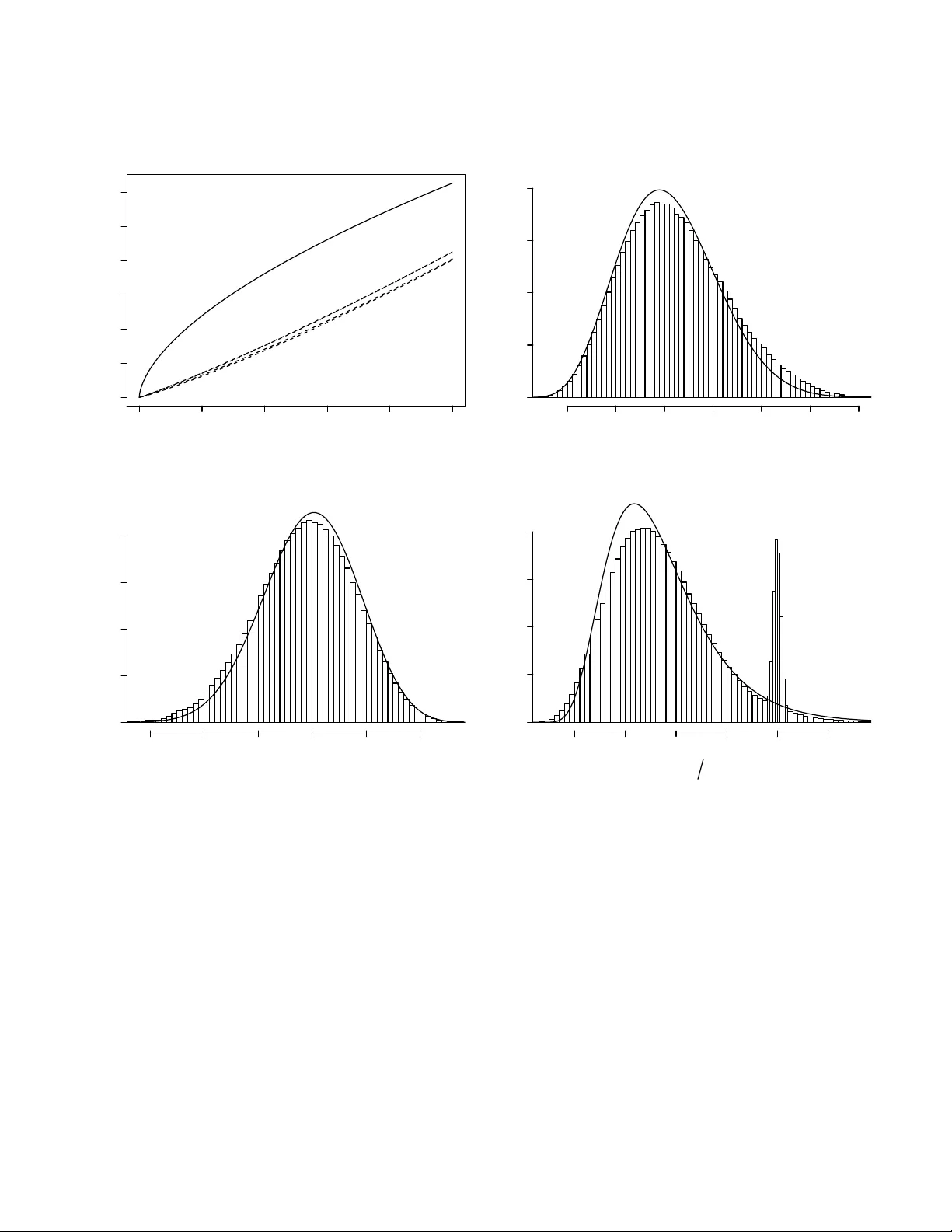
Sharp h yp otheses and bispatial inference Russell J. Bo w ater Indep endent r ese ar cher, Sartr e 47, A c atlima, Huajuap an de L e´ on, Oaxac a, C.P. 69004, Mexic o. Email addr ess: as given on arXiv.or g. Twitter pr oﬁle: @nake d statist Personal website: sites.go o gle.c om/site/b owaterfosp age Abstract: A fundamen tal class of inferen tial problems are those characterised b y there having b een a substan tial degree of pre-data (or prior) b elief that the v alue of a mo del parameter was equal or la y close to a sp eciﬁed v alue, which ma y , for example, b e the v alue that indicates the absence of an eﬀect. Standard w ays of tac kling problems of this t yp e, including the Bay esian metho d, are often highly inadequate in practice. T o address this issue, an inferential framew ork called bispatial inference is put forw ard, which can b e view ed as b oth a generalisation and radical rein terpretation of existing approac hes to inference that are based on P v alues. It is sho wn that to obtain an appropriate p ost-data density function for a given parameter, it is often conv enient to com bine a sp ecial t yp e of bispatial inference, whic h is constructed around one-sided P v alues, w ith a previously outlined form of ﬁducial inference. Finally , by using what are called p ost-data opinion curves, this bispatial-ﬁducial theory is naturally extended to deal with the general scenario in whic h an y n umber of parameters ma y b e unkno wn. The application of the theory is illustrated in v arious examples, which are esp ecially relev ant to the analysis of clinical trial data. Keyw ords: F oundational issues; Gibbs sampler; Organic ﬁducial inference; Parameter and sampling space h yp otheses; P ost-data opinion curv e; Pre-data kno wledge; Relativ e risk. 1 1. In tro duction Let us imagine that our aim is to mak e inferences ab out an unkno wn parameter ν on the basis of a data set x that w as generated b y a sampling model that dep ends on the true v alue of ν . Given this context, we will b egin with the following deﬁnition. Deﬁnition 1: Sharp and almost sharp h yp otheses The h yp othesis that the parameter ν lies in an in terv al [ ν 0 , ν 1 ] will be deﬁned as a sharp h yp othesis if ν 0 = ν 1 , and as an almost sharp hypothesis if the diﬀerence ν 1 − ν 0 is very small in the context of our general uncertain t y ab out ν after the data x hav e b een observed. Clearly , an y imp ortance attached to a h yp othesis of either of these tw o types should not generally hav e a great eﬀect on the wa y that w e mak e inferences ab out ν on the basis of the data x if there had b een no exceptional reason to b elieve that it would ha ve b een true or false b efore the data were observed. T aking this in to account, it will b e assumed that we are in the follo wing scenario. Deﬁnition 2: Scenario of in terest This scenario is c haracterised b y there having b een a substantial degree of b elief b efore the data were observed, i.e. a substantial pre-data b elief, that a giv en sharp or almost sharp h yp othesis ab out the parameter ν could ha ve b een true, but if, on the other hand, this h yp othesis had b een conditioned to b e false, i.e. if ν had b een conditioned not to lie in the interv al [ ν 0 , ν 1 ], then there w ould ha ve b een very little or no pre-data knowledge ab out this parameter o v er all of its allow able v alues outside of this in terv al. In this scenario, the hypothesis in question will b e referred to as the sp e cial h yp othesis. P erhaps some ma y try to dismiss the imp ortance of this t yp e of scenario, ho wev er trying to make data-based inferences ab out any giv en parameter of interest ν in such 2 a scenario represents one of the most fundamen tal problems of statistical inference that arise in practice. Let us consider the following examples. Example 1: In terv ening in a system If ν is a parameter of one part of a system, and an interv ention is made in a second part of the system that is arguably completely disconnected from the ﬁrst part, then there will b e a high degree of b elief that the v alue of ν will not change as a result of the in terv ention, i.e. there is a strong b elief in a sharp hypothesis ab out ν . Example 2: A randomised-con trolled trial Let us imagine that a sample of patients is randomly divided into a group of n t patien ts, namely the treatment group, that receiv e a new drug B, and a group of n c patien ts, namely the con trol group, that receiv e a standard drug A. W e will assume that e t patien ts in the treatmen t group exp erience a giv en adv erse ev en t, e.g. a heart attac k, in a certain p erio d of time follo wing the start of treatmen t, and that e c patien ts in the con trol group exp erience the same t yp e of ev en t in the same time p erio d. On the basis of this sample information, it will b e supp osed that the aim is to make inferences about the relative risk π t /π c , where π t and π c are the p opulation prop ortions of patien ts who would exp erience the adverse even t when given drug B and drug A resp ectiv ely . No w, if the action of drug B on the b o dy is very similar to the action of drug A, which is in fact often the case in practice when t w o drugs are b eing compared in this t yp e of clinical trial, then there ma y well hav e b een a strong pre-data b elief that this relative risk w ould b e close to one, or in other words, that the almost sharp hypothesis that the relativ e risk would lie in a narro w in terv al con taining the v alue one would b e true. It w ould app ear that a common wa y to deal with there ha ving b een a strong pre- data b elief that a sharp or almost sharp h yp othesis w as true is to simply ignore the incon v enient presence of this b elief. Ho wev er, doing so means that inferences based on 3 the observed data will often not b e even remotely honest. On the other hand, a formal metho d of addressing this issue that has received some atten tion is the Bay esian metho d. Let us take a quic k lo ok at ho w this metho d w ould w ork in a simple example. Example 3: Application of the Ba y esian metho d Let us supp ose that w e are interested in making inferences ab out the mean µ of a normal densit y function that has a kno wn v ariance σ 2 , on the basis of a sample of v alues x dra wn from the densit y function concerned. It will b e assumed that we are in the scenario of Deﬁnition 2 with the sp ecial hypothesis of in terest b eing the sharp hypothesis that µ = 0. Under the Ba yesian paradigm, it would b e natural to incorp orate any degree of pre-data b elief that µ equals zero into the analysis of the data by assigning a p ositive prior probability to this h yp othesis. Ho w ever, the only accepted wa y of expressing a lac k of kno wledge ab out a mo del pa- rameter under this paradigm is the con trov ersial strategy of placing a diﬀuse prop er or improp er prior density o v er the parameter concerned. T aking this in to accoun t, let us assume, without a great loss of generalit y , that the prior density function of µ conditional on µ 6 = 0 is a normal densit y function with a mean of zero and a large v ariance σ 2 0 . The inadequacy of the strategy in question is clearly apparent in the uncertaint y there w ould b e in c ho osing a v alue for the v ariance σ 2 0 , and this issue b ecomes very hard to conceal after appreciating that the amoun t of p osterior probabilit y giv en to the hypothesis that µ = 0 is highly sensitive to c hanges in this v ariance. F or example, the natural desire to allo w the v ariance σ 2 0 to tend to inﬁnity results in the p osterior probabilit y of this hypothesis tending to one for an y giv en data set x and any giv en p ositiv e prior probabilit y that is assigned to µ equalling zero. It can b e easily argued, therefore, that the application of standard Ba yesian theory 4 in the case just examined has an appalling outcome. Moreo ver, applying the Bay esian strategy just describ ed leads to outcomes of a similar type in cases where the sampling densit y of the data giv en the parameter of in terest ν is not normal, and/or the prior densit y of this parameter has a more general form, and also, imp ortantly , in cases where the sp ecial hypothesis is an almost sharp rather than, simply , a sharp h yp othesis. This clearly gives us a strong motiv ation to lo ok for an alternativ e metho d for making infer- ences ab out ν in the scenario of in terest. F ollo wing a similar path to that of Bow ater and Guzm´ an-P an to ja (2019b), the aim of the present pap er is to dev elop a satisfactory metho d for doing this on the basis of classical ideas ab out statistical inference. This metho d of inference will b e called bispatial inference. Before going further, let us summarise the structure of the pap er. In the next section, a general theory of bispatial inference is broadly outlined. A sp ecial formalisation of this theory is then developed in detail in Section 3. Given that all reasonable ob jectives for making inferences ab out a parameter of in terest ν can not b e conv eniently achiev ed by using this theory alone, a metho d of inference is put forward in Section 4 that is based on com bining bispatial inference with a sp eciﬁc t yp e of ﬁducial inference. In the ﬁnal main section of the pap er, namely Section 5, this combined theory is extended to cases where v arious mo del parameters are unknown. 2. General theory of bispatial inference 2.1. Ov erall problem Let us now consider a more general problem of statistical inference to the one that w as discussed in the In tro duction. In particular, w e now will be interested in the problem of making inferences ab out a set of parameters θ = { θ i : i = 1 , 2 , . . . , k } , where each θ i is a one-dimensional v ariable, on the basis of a data set x = { x i : i = 1 , 2 , . . . , n } that w as generated b y a sampling mo del that dep ends on this set of parameters. Let the join t 5 densit y or mass function of the data given the true v alues of the parameters θ b e denoted as g ( x | θ ). This will b e the ov erall problem of inference that we will b e concerned with in the rest of this pap er. 2.2. A note ab out probabilit y W e will in terpret the concept of probability under the deﬁnition of generalised sub jectiv e probabilit y that w as comprehensiv ely outlined in Bo water (2018b). Giv en that it will not b e necessary to explicitly discuss this deﬁnition of probability in the present pap er, the reader is referred to this earlier w ork for further information. Nevertheless, in relation to the general topic in question, there is a sp eciﬁc issue that should not b e ov erlo oked. In particular, w e observ e that when ev en ts are rep eatable, the concept of the probabilit y of an even t and the concept of the prop ortion of times the ev ent o ccurs in the long term are often used in terc hangeably . Ho w ever, this is not alwa ys appropriate. The reason for this is that a p opulation prop ortion is a fact ab out the physical world, while under certain deﬁnitions of probabilit y , e.g. the deﬁnition that will b e adopted here, a probability is primarily alwa ys a measure of a giv en individual’s state of mind. Therefore, where necessary , w e will denote the p opulation prop ortion of times any giv en ev ent A o ccurs b y ρ ( A ), while the probability of the ev en t A will, as usual, b e denoted by P ( A ). 2.3. P arameter and sampling space h yp otheses The theory of inference that will be developed is based on a h yp othesis H P that concerns an even t in the parameter space, and an equiv alen t hypothesis H S that is stated in terms of the prop ortion of times an ev en t in the sampling space will o ccur in the long run. The link that is made betw een the parameter and sampling spaces through the atten tion giv en to these tw o h yp otheses is the reason that this type of inference will b e called bisp atial inference. More sp eciﬁcally , these tw o t yp es of h yp othesis will b e assumed to hav e the 6 follo wing deﬁnitions. Deﬁnition 3: P arameter space h yp othesis H P Giv en that, from now, H : C will denote the hypothesis H that a given condition C is true, the parameter space hypothesis H P is deﬁned by: H P : θ ∈ Θ 0 where Θ 0 is a given subset of the en tire space Θ o ver which the set of parameters θ is deﬁned. Deﬁnition 4: Sampling space h yp othesis H S The tw o conditions that the sampling space h yp othesis H S m ust satisfy are: 1) It m ust b e equiv alen t to the hypothesis H P , i.e. if H S is true then H P m ust b e true and if H P is true then H S m ust b e true. 2) It must hav e the follo wing form: H S : ρ ( J ( X ∗ ) ∈ J 0 ( x )) ∈ P 0 where J ( X ∗ ) is a statistic calculated on the basis of an as-yet-unobserv ed second sample X ∗ of v alues dra wn from the density function g ( x | θ ), which is p ossibly of a diﬀeren t size to the observed (ﬁrst) sample x , the set J 0 ( x ) is a given subset of the en tire space J o ver whic h the statistic J ( X ∗ ) is deﬁned, and the set P 0 is a giv en subset of the interv al [0 , 1]. T o clarify , the h yp othesis H S is the hypothesis that the unknown population prop ortion ρ ( J ( X ∗ ) ∈ J 0 ( x )) lies in the known set P 0 . Also, it should b e clariﬁed that the deﬁnition of the set J 0 ( x ) will dep end, in general, on the data set x . 7 2.4. Inferen tial pro cess It will be assumed that inferences are made ab out the set of parameters θ b y pro ceeding through the steps of the following algorithm: Step 1: F ormation of a suitable hypothesis H P . The choice of this hypothesis should b e made with the goal in mind of b eing able to make useful inferences ab out the parame- ters θ . Step 2: Assessmen t of the likeliness of the h yp othesis H P b eing true using only pre-data kno wledge ab out the parameters θ . It is not necessary that this assessment is expressed in terms of a formal measure of uncertaint y , e.g. a probabilit y do es not need to b e assigned to this hypothesis. Step 3: F ormation of a suitable h yp othesis H S . Step 4: Assessmen t of the lik eliness of the hypothesis H S b eing true after the data x hav e b een observ ed. In carrying out this assessment, all relev ant factors ought to b e tak en in to account including, in particular, the assessmen t made in Step 2 and the known equiv alency b etw een the hypotheses H P and H S . Step 5: Conclusion ab out the likeliness of the hypothesis H P b eing true ha ving tak en in to account the data x . This is directly implied b y the assessment made in Step 4 due to the equiv alence of the hypotheses H P and H S . 2.5. First example: Tw o-sided P v alues In the next three sections, we will apply the metho d outlined in the previous section to the problem of inference referred to in Example 3 of the Introduction, i.e. that of making inferences ab out a normal mean µ when the p opulation v ariance σ 2 is known. In this case, it is clear that the set of unkno wn parameters θ will consist of just the mean µ . 8 T o giv e a context to this problem, let us imagine that a patien t is b eing constantly monitored with regard to the concen tration of a certain c hemical in his/her blo o d. W e will assume that the measuremen ts of this concentration are notably imprecise, and in particular, it will b e assumed that any such measuremen t follo ws a normal density function with known v ariance σ 2 / 2 centred at the true concentration. Also, let us sup- p ose that the data x is simply the measurement of this concentration at a time p oint t 2 min us the same t yp e of measurement taken at a time p oint t 1 , where the time p oint t 1 is immediately b efore the patient is sub jected to some kind of in terv ention and the time p oin t t 2 is immediately after this interv ention. No w, if the in terven tion in question w ould not b e expected to aﬀect the concen tration of the c hemical of in terest, there is lik ely to b e a substan tial degree of pre-data belief that the true c hange in this concentration in going from the time p oint t 1 to the time p oint t 2 , namely the change µ in this concentration, will b e v ery small. In fact, to b egin with, let us assume that these tw o time p oints are so close together that w e ﬁnd ourselv es in the scenario of Deﬁnition 2 with the sp ecial hypothesis b eing the sharp hypothesis that µ = 0. It can b e seen therefore that we ha v e eﬀectively arriv ed at a sp eciﬁc form of Example 1 of the Introduction. Under the assumptions that hav e b een made, it is reasonable, as part of Steps 1 and 3 of the algorithm of Section 2.4, to deﬁne the hypotheses H P and H S as follows: H P : µ = 0 H S : ρ ( { X ∗ < −| x | } ∪ { X ∗ > | x | } ) = 2Φ( −| x | /σ ) (1) where X ∗ is equal to an additional unobserv ed measurement of the concentration in question tak en at time t 2 min us an additional unobserved measuremen t of the same type tak en at time t 1 , while Φ( y ) is the cumulativ e density of a standard normal distribution at the v alue y . It can b e easily appreciated that these tw o hypotheses are in fact equiv- alen t. Observ e that the quantit y on the righ t-hand side of the equality in equation (1) 9 w ould b e the standard t w o-sided P v alue that w ould b e calculated on the basis of the observ ation x if H P w as regarded as b eing the null h yp othesis. No w, in Step 4 of the algorithm of Section 2.4, although a small v alue for this t w o- sided P v alue would naturally disfa v our the h yp othesis H S , and in particular fav our the left-hand side of the equalit y in equation (1) b eing greater than this P v alue, this w ould need to b e balanced b y how muc h the pre-data assessment in Step 2 of this algorithm fa v oured the h yp othesis H P . Nevertheless, if the P v alue under discussion turns out to b e v ery small then, ev en if the h yp othesis H P w as quite strongly fa voured b efore the data v alue x was observ ed, it ma y well b e regarded as b eing rational to decide that hypothesis H S is fairly unlik ely to b e true. As will alwa ys b e the case, the ev aluation of the lik eliness of the h yp othesis H P in Step 5 of the algorithm in question should b e the same as the ev aluation of the likeliness of the hypothesis H S in Step 4 of this algorithm. 2.6. Second example: Q v alues Let us now consider the more general case of the example b eing curren tly examined where the sp ecial h yp othesis in the scenario of Deﬁnition 2 is the almost sharp hypothesis that µ lies in the interv al [ − ε, ε ], where ε is a small p ositive constan t. In this case, it is reasonable to deﬁne the hypotheses H P and H S as follows: H P : µ ∈ [ − ε, ε ] H S : ρ ( { X ∗ < −| x | } ∪ { X ∗ > | x | } ) ≤ q ( ε ) where q ( ε ) = Φ(( −| x | − ε ) /σ ) + Φ(( −| x | + ε ) /σ ) (2) It can easily b e shown that these tw o hypotheses are equiv alent under the assumptions that ha v e b een made. Notice that the v alue q ( ε ) as sp eciﬁed in equation (2) would b e classiﬁed as the Q v alue for the hypothesis that µ = ε according to the general deﬁnition 10 of a Q v alue that was presen ted and discussed in Bo water and Guzm´ an-P an to ja (2019b), and therefore here will also b e referred to as a Q v alue. Similar to the previous example, although w e w ould naturally disfa vour the h yp othesis H S , and as a result, the h yp othesis H P if this Q v alue w as small, this would need to b e balanced by how m uc h the hypothesis H P w as fav oured b efore the v alue x w as observed in order to make a sensible ev aluation of the likeliness of the hypothesis H S b eing true. 2.7. Third example: One-sided P v alues T o give another example, let us lo ok at an alternativ e wa y of deﬁning the hypotheses H P and H S in the context of the sp eciﬁc problem of inference that is currently under discussion. In particular, let us now assume that, if x ≤ 0, then these hypotheses would b e deﬁned as: H P : µ ≥ − ε (3) H S : ρ ( X ∗ < x ) ≤ Φ(( x + ε ) /σ ) (4) while if x > 0, then they would ha v e the deﬁnitions: H P : µ ≤ ε (5) H S : ρ ( X ∗ > x ) ≤ Φ(( − x + ε ) /σ ) (6) Again, it can b e easily shown that the hypotheses H P and H S in equations (3) and (4) are equiv alen t, and also that these h yp otheses as deﬁned in equations (5) and (6) are equiv alen t. In addition, observe that the quantities on the righ t-hand sides of the in- equalities in equations (4) and (6) would b e the standard one-sided P v alues that would b e calculated on the basis of the observ ation x if the null hypotheses were regarded as b eing the hypotheses H P that corresp ond to the h yp otheses H S deﬁned in these t w o equations. 11 Clearly , the substantial degree of pre-data b elief that µ lies in the interv al [ − ε, ε ] should b e reﬂected in the pre-data assessment of the likeliness of the hypothesis H P as deﬁned in either equation (3) or equation (5). F urthermore, similar to what w as seen in the previous examples, a substantial degree of pre-data b elief in whichev er one of the h yp otheses H P in these equations is applicable would need to b e appropriately balanced b y the information represen ted by the observ ation x that is summarised by the one-sided P v alue that app ears in the corresp onding h yp othesis H S , in order to make an adequate assessmen t of the likeliness of this latter h yp othesis giv en the observ ed v alue of x . 2.8. Discussion of examples Although the metho ds that ha v e just b een outlined in Sections 2.5 to 2.7 can b e applied to man y other problems of inference than the simple one that has b een considered, the latter metho d based on one-sided P v alues is muc h more widely applicable than the former t w o metho ds based on tw o-sided P v alues and on Q v alues, in particular, it is able to cop e b etter with sampling densities that are m ultimo dal and/or non-symmetric. Also, it can be argued, not just in terms of the speciﬁc problem that has b een discussed but more generally , that it is going to be less easy to ev aluate, on the whole, the lik eliness of hypotheses H S that are based either on tw o-sided P v alues or on Q v alues than those that are based on one-sided P v alues. With regard to the examples that ha v e b een presen ted, a simple observ ation that underlies the argument b eing referred to is that, for an y giv en v alue of x , one of the t w o op en in terv als ov er whic h either a t wo-sided P v alue or a Q v alue is determined b y integration of the sampling densit y , i.e. one of the in terv als ( −∞ , −| x | ) or ( | x | , ∞ ), will contain a prop ortion of the sampling density that alw a ys decreases in size as the mean µ mo v es aw ay from zero, despite of course this c hange in µ alwa ys causing the total prop ortion of the sampling density con tained in these tw o in terv als to increase. 12 F or the reasons that hav e just b een giv en, we will not consider generalising in a formal w a y the metho ds based on t wo-sided P v alues and on Q v alues that were put forward in Sections 2.5 and 2.6. Instead, the type of metho d based on one-sided P v alues that w as describ ed in Section 2.7 and dev elopments of this metho d, will constitute the main form of bispatial inference that will b e explored in the rest of this pap er. It should b e p oin ted out that, although it is apparent from the example considered in Section 2.7 that p ossibly an imp ortant dra wback of this metho d is that, in the scenario of Deﬁnition 2, it will not generally allo w us to directly assess the lik eliness of the sp ecial hypothesis that a parameter of in terest ν lies in a narrow in terv al [ ν 0 , ν 1 ] after the data ha ve been observed, i.e. that µ lies in the in terv al [ − ε, ε ] in the example in question, it will b e shown later ho w this diﬃculty can b e ov ercome. 3. Sp ecial form of bispatial inference 3.1. General assumptions Let us now formalise the sp eciﬁc type of bispatial inference that has just b een iden tiﬁed. F or the moment, it will b e assumed that the only unknown parameter on which the sampling density g ( x | θ ) dep ends is the parameter θ j , either b ecause there are no other parameters in the mo del, or b ecause all the other parameters are kno wn. Also, w e will assume that the scenario of interest is again the scenario outlined in Deﬁnition 2, with the unknown parameter now b eing of course θ j , and that, in this scenario, the sp ecial h yp othesis is the almost sharp hypothesis that θ j lies in the narrow in terv al [ θ j 0 , θ j 1 ]. 3.2. T est statistic Let us b egin by detailing ho w the concept of a test statistic will be interpreted. In particular, it will b e assumed that a test statistic T ( x ), whic h will also b e denoted 13 simply by the v alue t , satisﬁes the following tw o requiremen ts: 1) Similar to what in Bo w ater (2019a) was deﬁned as b eing a ﬁducial statistic, it is necessary that the test statistic T ( x ) is a univ ariate statistic of the sample x that can b e regarded as eﬃcien tly summarising the information that is contained in this sample ab out the parameter θ j , given the v alues of other statistics that do not pro vide any information ab out this parameter, i.e. ancillary statistics. 2) Let F ( t | θ j , u ) be the cum ulativ e distribution function of the unobserv ed test statistic T ( X ) ev aluated at its observ ed v alue t given a v alue for the parameter θ j , and conditional on U ( X ) b eing equal to u , where u are the observed v alues of an appropriate set of ancillary statistics U ( X ) of the data set of interest, i.e. F ( t | θ j , u ) equals the probabilit y P ( T ( X ) ≤ t | θ j , u ), and also let F 0 ( t | θ j , u ) = P ( T ( X ) ≥ t | θ j , u ). On the basis of this notation, it is necessary that, ov er the set of allo w able v alues for θ j , the probabilities F ( t | θ j , u ) and 1 − F 0 ( t | θ j , u ) strictly decrease as θ j increases. As far as the examples that will b e considered in this pap er are concerned, condition (1) will b e satisﬁed, in a simple and clear-cut manner, b y T ( x ) b eing a univ ariate suﬃcient statistic for θ j . As a result, the set of ancillary statistics U ( x ) referred to in condition (2) will naturally be assigned to b e empt y in these examples, and in fact w e could reasonably exp ect that it would usually be appropriate to assign this set to b e empt y when the c hoice of the test statistic T ( x ) is more general. 3.3. P arameter and sampling space h yp otheses If the condition F ( t | θ j = θ j 0 , u ) ≤ F 0 ( t | θ j = θ j 1 , u ) (7) holds, where the v alues θ j 0 and θ j 1 are as deﬁned in Section 3.1, then the hypotheses H P and H S will b e deﬁned as: 14 H P : θ j ≥ θ j 0 (8) H S : ρ ( T ( X ∗ ) ≤ t | u ) ≤ F ( t | θ j = θ j 0 , u ) (9) where X ∗ is again an as-y et-unobserv ed sample of v alues drawn from the densit y function g ( x | θ ) but no w this sample will b e assumed to b e alw ays of the same size as the ob- serv ed sample x , i.e. it m ust consist of n observ ations, and where ρ ( T ( X ∗ ) ≤ t | u ) is the unkno wn p opulation prop ortion of times that T ( X ∗ ) ≤ t conditional on the ancillary statistics U ( x ) calculated on the basis of the data set X ∗ b eing equal to the v alues u , i.e. conditional on U ( X ∗ ) = u . On the other hand, if the condition in equation (7) do es not hold, then the hypotheses in question will b e deﬁned as: H P : θ j ≤ θ j 1 (10) H S : ρ ( T ( X ∗ ) ≥ t | u ) ≤ F 0 ( t | θ j = θ j 1 , u ) (11) Giv en the w a y that the test statistic T ( x ) was deﬁned in Section 3.2, it can b e easily appreciated that the hypotheses H P and H S in equations (8) and (9) are equiv alent, and also that these h yp otheses as deﬁned in equations (10) and (11) are equiv alent. In addition, observ e that the probabilities F ( t | θ j = θ j 0 , u ) and F 0 ( t | θ j = θ j 1 , u ) that app ear in the deﬁnitions of the hypotheses H S in equations (9) and (11) would b e the standard one-sided P v alues that w ould b e calculated on the basis of the data set x if the n ull hypotheses were regarded as being the hypotheses H P that corresp ond to the tw o h yp otheses H S in question. W e will assume that to make inferences ab out the parameter of interest θ j , the same algorithm will b e used as was outlined in Section 2.4. How ever, with regard to the use of this algorithm in the current con text, let us make the follo wing commen ts: a) The set of parameters θ referred to in this algorithm will of course consist of only the parameter θ j . 15 b) In Step 2 of this algorithm, it is evident that some sp ecial attention will often need to b e placed in assessing the likeliness of the almost sharp h yp othesis that θ j lies in the in terv al [ θ j 0 , θ j 1 ] based on only pre-data kno wledge ab out θ j , since w e can see that this hypothesis will alw a ys b e included in the hypothesis H P , but will not generally b e equiv alen t to H P . c) In assessing the likeliness of the h yp othesis H S in Step 4 of this algorithm, one of the relev an t factors that ough t to b e tak en in to accoun t is clearly the size of the one-sided P v alue that app ears in the deﬁnition of this h yp othesis, i.e. the v alue F ( t | θ j = θ j 0 , u ) or the v alue F 0 ( t | θ j = θ j 1 , u ). d) Also in Step 4 of this algorithm, it now will b e assumed that the goal is usually to assign a probability to the h yp othesis H S . With reference to this last commen t, the task of assigning a probabilit y to the hypoth- esis H S ma y b e made easier by ﬁrst trying to determine what would b e the minim um probabilit y that could b e sensibly assigned to this h yp othesis. In particular, for a reason that should b e obvious, it would not seem sensible to assign a probability to the hy- p othesis H S that is less than the probabilit y that w ould b e assigned to this hypothesis if nothing or very little had b een kno wn ab out the parameter θ j b efore the data w ere ob- serv ed. One w ay , but not as y et a widely accepted wa y , of making inferences ab out θ j in this latter t yp e of situation is to use the ﬁducial metho d of inference (whic h has its origins in Fisher 1935 and Fisher 1956) and, given the interpretation of the concept of proba- bilit y b eing relied on in the presen t pap er (see Section 2.2), it would seem appropriate to consider applying the form of this t yp e of inference that has b een called sub jective, or more recently , organic ﬁducial inference, see Bow ater (2017), Bo w ater (2018a) and Bo w ater (2019a). In this regard, let P f ( H S ) denote the p ost-data or ﬁducial probabilit y that would b e assigned to the h yp othesis H S as a result of applying this latter metho d of ﬁducial inference if there had been no or v ery little pre-data kno wledge ab out θ j . There- 16 fore, this v alue P f ( H S ) can b e considered as b eing a minimum v alue for the p ost-data probabilit y of the h yp othesis H S b eing true in the genuine scenario of interest, i.e. the scenario of Deﬁnition 2. This metho d for placing a p otentially useful lo w er limit on the probabilit y of the h yp othesis H S will b e illustrated as a feature of the examples that will b e describ ed in the next t wo sections. 3.4. First example: Inference ab out a normal mean with v ariance kno wn Let us return to the example that w as discussed in Section 2.7. W e can see that this example ﬁts within the sp ecial framework for bispatial inference that has just b een out- lined. In particular, the v alue x , i.e. the observ ed c hange in concentration, is clearly a suitable test statistic T ( x ), since it is a suﬃcient statistic for the mean µ that will satisfy condition (2) of Section 3.2 for any v alue it may p ossibly tak e. Also, the w a y that the h yp otheses H P and H S w ere sp eciﬁed in Section 2.7 matc hes ho w these h yp otheses would b e sp eciﬁed by using the deﬁnitions in Section 3.3. In this earlier example, let us no w more speciﬁcally assume that σ = 1, ε = 0 . 2 and x = 2 . 7. Under these assumptions, the relev ant h yp otheses H P and H S are as giv en in equations (5) and (6), and the one-sided P v alue on the right-hand side of the inequalit y in equation (6) is 0.0062. Since this P v alue is obviously small, but not v ery small, if a substan tial probabilit y of around 0 . 3 would ha ve b een placed on the h yp othesis that µ ∈ [ − 0 . 2 , 0 . 2] b efore the v alue x was observed, it w ould seem p ossible to justify a probability in the range of sa y 0.03 to 0.08 b eing placed on the hypothesis H S : ρ ( X ∗ > 2 . 7) ≤ 0 . 0062 b eing true, and as a result, on the hypothesis H P : µ ≤ 0 . 2 b eing true after the v alue x has b een observ ed. The probabilit y that w ould b e assigned to this h yp othesis H P after the v alue x has b een observ ed b y applying the strong ﬁducial argument (see Bo w ater 2019a) as part of the metho d of organic ﬁducial inference would b e equal to 0.0062, i.e. the one-sided 17 P v alue of in terest. W e therefore can regard the probability P f ( H S ) referred to in the last section as b eing equal to 0.0062 in this example. Since the form of reasoning under discussion could be considered as justifying this v alue of 0.0062 as b eing a minimum v alue for the probability of the h yp othesis H S in the genuine scenario of in terest, it is therefore appropriate that the range of v alues for this probability that has b een prop osed is w ell ab o v e this minim um v alue. 3.5. Second example: Inference ab out a binomial prop ortion Let us imagine that a random sample of patients are switched from b eing giv en a standard drug A to b eing given a new drug B. After a p erio d of time has passed, they are asked whic h out of the t w o drugs A and B they prefer. The prop ortion of patien ts who prefer drug B to drug A, after patien ts who do not express a preference hav e b een excluded, will b e denoted by the v alue b . Given this sample proportion, it will b e assumed that the aim is mak e inferences ab out its corresp onding p opulation prop ortion π . F or a similar reason with regard to the nature of drugs A and B as that giv en in Example 2 of the In tro duction, let us also supp ose that the scenario of Deﬁnition 2 applies with the sp ecial h yp othesis b eing the hypothesis that the prop ortion π lies in a narro w interv al centred at 0.5, which will b e denoted as [0 . 5 − ε, 0 . 5 + ε ]. Observ e that the sample prop ortion b clearly satisﬁes the requirements of Section 3.2 to b e a suitable test statistic T ( x ). T o give a more sp eciﬁc example, we will assume that there are tw elve patien ts in the sample, of whom nine prefer drug A to drug B, one prefers drug B to drug A and t w o do not express a preference, and therefore b = 0 . 1. Also, let the constant ε b e equal to 0.03. It no w follo ws that, under the deﬁnitions of Section 3.3, the hypotheses H P and H S w ould b e sp eciﬁed as: H P : π ≥ 0 . 47 H S : ρ ( B ∗ ≤ 0 . 1) ≤ 0 . 53 10 + 10(0 . 47)(0 . 53 9 ) = 0 . 0173 (12) 18 where B ∗ is the prop ortion of patients who would prefer drug B to drug A in an as-yet- unobserv ed sample of ten patients who express a preference b etw een the tw o drugs. W e can see that again the one-sided P v alue, i.e. the v alue 0.0173 in equation (12), is reasonably small. Therefore, if a pre-data probability of say 0.3 w ould hav e b een placed on the hypothesis that π ∈ [0 . 47 , 0 . 53], it would seem p ossible to justify a probability in the range of say 0.03 to 0.08 b eing placed on the hypothesis H S b eing true, and as a result, on the hypothesis H P b eing true after the prop ortion b has b een observ ed. The probabilit y that would b e assigned to the h yp othesis H P after the v alue b has b een observ ed b y using the strong ﬁducial argumen t, and a local pre-data (LPD) function for π (see Bo water 2019a) deﬁned by: ω L ( π ) = c for all π ∈ [0 , 1] (13) where c is a p ositive constant, as part of the metho d of organic ﬁducial inference w ould b e equal to 0.0070. Since this post-data probabilit y can justiﬁably be regarded as the probabilit y P f ( H S ) referred to Section 3.3, and therefore as b eing a minimum v alue for the probabilit y of the h yp othesis H S in the gen uine scenario of in terest, it is appropriate that, similar to the previous example, the range of v alues for the probability of this h yp othesis that has b een prop osed is well ab ov e this minim um v alue. 3.6. F oundational basis of the theory In the examples considered in the previous section and Section 3.4, it was inherently assumed that the smaller the size of the one-sided P v alue that appears in the h yp othesis H S , the less inclined we should b e to b eliev e that this hypothesis is true. How ever, what is the foundational basis for this assumption? W e will no w try to oﬀer s ome kind of answ er to this question. It can b e seen that the tw o versions of the hypothesis H S in equations (9) and (11) 19 can b oth b e represented as: H S : ρ ( A ) ≤ β (14) where A is a given condition and β is a given one-sided P v alue. Therefore, the p opu- lation prop ortion of times condition A is satisﬁed will b e less than or equal to β if the corresp onding h yp othesis H P is true, or in other words, if the parameter θ j is restricted in the wa y that is sp eciﬁed by this latter hypothesis. How ever, w e could also calculate a p ost-data probability for condition A b eing satisﬁed without placing restrictions on the parameter θ j b y using the ﬁducial argumen t. In particular, the p ost-data probability in question would b e deﬁned as: P f ( A ) = Z A Z ∞ −∞ g ( X ∗ | θ j , u ) f ( θ j | x ) dθ j dX ∗ (15) where f ( θ j | x ) is an appropriate ﬁducial densit y function for the parameter θ j . T o clarify , the outer integral in this equation is o v er unobserv ed data sets X ∗ that satisfy condi- tion A . It will b e helpful if we no w lo ok at a sp eciﬁc example, and so let us again consider the example discussed in Sections 2.7 and 3.4. In this case, the ﬁducial density of the parameter of in terest µ , i.e. the densit y f ( µ | x ), obtained by using the strong ﬁducial argumen t is deﬁned by the expression µ ∼ N( x, σ 2 ). On the basis of this ﬁducial density for µ , it is simple to show, by using equation (15), how we obtain the result that P f ( A ) equals 0 . 5 for any given observed v alue of x , where as we know A = { X ∗ < x } or A = { X ∗ > x } , which of course is a sp ecial result that in fact could hav e b een derived by using more direct ﬁducial reasoning. W e could in terpret this result as meaning that the probabilit y that we should assign to condition A b eing true if we had known nothing or v ery little ab out µ b efore the v alue x was observed should b e 0.5. T aking into account this interpretation, if we were to prop ose assigning a large prob- 20 abilit y to the hypothesis H S b eing true when the P v alue β in equation (14) was quite small, then it w ould seem fair if w e were asked how we can justify doing this given the large diﬀerence b etw een this P v alue and the probabilit y P f ( A ). T o be able to giv e a satisfactory answ er to this question, it is reasonable to argue that the only situation we could be in would b e one in whic h, b efore the v alue x was observed, there had b een a high degree of b elief that the hypothesis H P w as true, whic h in the con text of the scenario of Deﬁnition 2, w ould mean a high degree of pre-data b elief that µ lay in the in terv al [ − ε, ε ]. In this situation, we could argue that assigning a large probability to the hypothesis H S when the P v alue β is quite small can b e justiﬁed due to the imp ortance that is attached to the probabilit y P f ( A ) as a b enchmark or reference v alue b eing greatly diminished as a result of our strong pre-data opinion ab out µ . F urthermore, let us supp ose that a given probabilit y of α 0 w ould b e assigned to the h yp othesis H S b eing true if the P v alue β was equal to a giv en v alue β 0 that is less than sa y 0.05. Now, if w e imagine a scenario in whic h the v alue of β is less than β 0 , and therefore further aw ay from the probabilit y P f ( A ) than β 0 , then it can b e easily argued that the only w a y we could justify assigning the same probability α 0 to the h yp othesis H S w ould b e if, for an unrelated reason, it was decided that our pre-data b elief that µ ∈ [ − ε, ε ] should b e increased. Also, it is fairly uncon trov ersial to argue that for any ﬁxed data v alue x , the degree of pre-data b elief that µ ∈ [ − ε, ε ] and the degree of p ost- data belief in the h yp othesis H P should be positively correlated. As a logical consequence of these arguments, it follo ws that, if there is a ﬁxed degree of pre-data b elief that µ ∈ [ − ε, ε ], then the probabilit y w e should wish to assign to the h yp othesis H S after the v alue x has been observ ed should decrease as the v alue that the P v alue β is assumed to take is made smaller, on condition that this P v alue is already small. Therefore, w e hop e that an adequate answer to the question posed at the start of this section has b een pro vided. 21 Another foundational issue that no doubt some w ould try to raise cen tres on the argumen t that the probability that is assigned, on the basis of the observ ed data, to the hypothesis H S as part of the metho d that has b een outlined should b e treated as a p osterior probabilit y that corresponds to the Bay esian update of some giv en prior densit y function for the parameter of in terest θ j , where the c hoice for this prior densit y , of course, do es not dep end on the data. Ho w ev er, to b e able to sensibly use the Bay esian metho d b eing referred to some justiﬁcation would need to b e given as to wh y such a prior densit y function w ould hav e b een a go od representation of our beliefs ab out the parameter θ j b efore the data were observed. The fact that, in the con text of the scenario of in terest in Deﬁnition 2, it is going to b e extremely diﬃcult, in general, to pro vide suc h a justiﬁcation is consistent with the motiv ation for the metho d of bispatial inference that was given in the Introduction. 4. Bispatial-ﬁducial inference The metho dology of Sections 3.1 to 3.3 allo ws us to determine a p ost-data probabilit y for the h yp othesis H P b eing true. Clearly though, it would be preferable to hav e a p ost-data densit y function for the parameter of interest θ j . F or this reason, let us no w consider generalising the metho dology that has b een prop osed. In particular, if F ( t | θ j = θ j ∗ , u ) ≤ F 0 ( t | θ j = θ j ∗ , u ) where θ j ∗ is any given v alue of θ j , then let us deﬁne the h yp otheses H P and H S as: H P : θ j ≥ θ j ∗ H S : ρ ( T ( X ∗ ) ≤ t | u ) ≤ F ( t | θ j = θ j ∗ , u ) , (16) otherwise, we will deﬁne these h yp otheses as: 22 H P : θ j ≤ θ j ∗ H S : ρ ( T ( X ∗ ) ≥ t | u ) ≤ F 0 ( t | θ j = θ j ∗ , u ) (17) W e can observe that a p ost-data distribution function for θ j could b e constructed if, for eac h v alue of θ j ∗ within the range of allo wable v alues for θ j , w e were able to consisten tly ev aluate the p ost-data probability of the hypothesis H S that is applicable as deﬁned by either equation (16) or (17). Obviously , it w ould be a little a wkward to do this b y directly assessing the lik eliness of the h yp othesis H S b eing true for all the v alues of θ j ∗ concerned, ho w ever no assumption has b een made regarding whether assessmen ts of this t yp e should b e made directly or indirectly . Therefore, we now will consider a strategy in which only one of these probabilit y assessmen ts is made directly , while all the other assessments of this type that are required will in eﬀect b e made indirectly b y using again the metho d of organic ﬁducial inference. The application of this general strategy will b e referred to as bispatial-ﬁducial inference. 4.1. First prop osed metho d Under the assumption that the hypothesis H S satisﬁes the more con v entional deﬁnition of this type of h yp othesis giv en in Section 3.3, let us assume that, after the data hav e b een observed, we directly weigh up, and then determine a v alue for the probability of this hypothesis b eing true. This p ost-data probabilit y will b e denoted by the v alue α , i.e. P ( H S ) = α . F urthermore, it will b e assumed that the metho d of organic ﬁducial inference is used to derive a ﬁducial density function for θ j conditional on θ j not lying in the interv al [ θ j 0 , θ j 1 ]. In this approach to inference, the global pre-data (GPD) function ω G ( ν ) (see Bo w ater 2019a) oﬀers the principal, if not exclusiv e, means b y whic h pre-data b eliefs ab out a parameter of interest ν can b e expressed. Giv en that it is b eing assumed that, under the condition that θ j do es not lie in the in terv al [ θ j 0 , θ j 1 ], nothing or v ery little 23 w ould hav e b een known ab out θ j b efore the data w ere observ ed, it is appropriate to use a neutral GPD function for θ j that has the following form: ω G ( θ j ) = ( 0 if θ j ∈ [ θ j 0 , θ j 1 ] d otherwise (18) where d > 0. On the basis of this GPD function, the ﬁducial densit y function of θ j that is of interest can often b e deriv ed b y applying what, in Bo water (2019a), w as referred to as the mo derate ﬁducial argument (when Principle 1 of this earlier pap er can b e applied). Alternativ ely , in accordance with what was also adv o cated in Bo w ater (2019a), this ﬁducial density can b e more generally deﬁned, with resp ect to the same GPD function for θ j , by the following expression: f ( θ j | θ j / ∈ [ θ j 0 , θ j 1 ] , x ) = C 0 f S ( θ j | x ) (19) where C 0 is a normalising constant, and f S ( θ j | x ) is a ﬁducial density for θ j deriv ed by applying the strong ﬁducial argument (as part of what is required b y either Principle 1 or Principle 2 of Bow ater 2019a) that would b e regarded as b eing a suitable ﬁducial density for θ j in a general scenario where it is assumed that there w as no or v ery little pre-data kno wledge ab out θ j o v er all p ossible v alues of θ j . Giv en the assumptions that hav e been made, if the condition in equation (7) holds, whic h implies that H P is the h yp othesis that θ j ≥ θ j 0 , then it can b e deduced that the p ost-data probability of the even t θ j ∈ [ θ j 0 , θ j 1 ] is deﬁned by: P ( θ j ∈ [ θ j 0 , θ j 1 ] | x ) = α − λ (1 − α ) (20) where the probability α is as deﬁned at the start of this section, and λ is giv en b y: λ = P f ( θ j > θ j 1 | θ j / ∈ [ θ j 0 , θ j 1 ] , x ) P f ( θ j < θ j 0 | θ j / ∈ [ θ j 0 , θ j 1 ] , x ) where P f ( A | θ j / ∈ [ θ j 0 , θ j 1 ] , x ) denotes the ﬁducial probability of the even t A conditional 24 on θ j / ∈ [ θ j 0 , θ j 1 ] that is the result of in tegrating the ﬁducial densit y f ( θ j | θ j / ∈ [ θ j 0 , θ j 1 ] , x ) sp eciﬁed by equation (19) ov er those v alues of θ j that satisfy the condition A . Under the condition in equation (7), it also follows that the p ost-data densit y function of θ j , whic h will b e denoted simply as p ( θ j | x ), is deﬁned ov er all of its domain except for the in terv al [ θ j 0 , θ j 1 ] by the expression: p ( θ j | x ) = ( (1 − α ) f ( θ j | { θ j < θ j 0 } , x ) if θ j < θ j 0 λ (1 − α ) f ( θ j | { θ j > θ j 1 } , x ) if θ j > θ j 1 (21) where f ( θ j | B , x ) denotes the ﬁducial density f ( θ j | θ j / ∈ [ θ j 0 , θ j 1 ] , x ) sp eciﬁed b y equa- tion (19) conditioned on the even t B . T o clarify , the density p ( θ j | x ) is b eing referred to as a p ost-data density b ecause o v er the restricted space for θ j in question it is deﬁned on the basis of the p ost-data probabilit y of the hypothesis H S , i.e. the v alue α , and the ﬁducial density f ( θ j | θ j / ∈ [ θ j 0 , θ j 1 ] , x ), which of course is a particular type of p ost-data densit y . While it has b een assumed that the condition in equation (7) holds, it should b e obvious, on the basis of symmetry , how to modify the deﬁnitions in equations (20) and (21) in cases where this condition does not hold, i.e. when H P is the h yp othesis that θ j ≤ θ j 1 . Notice that the assignment of a probability α to the hypothesis H S that is greater than or equal to the minimum v alue P f ( H S ) for this probability that w as referred to at the end of Section 3.3 is a suﬃcient (but not a necessary) requiremen t for ensuring that the probabilit y P ( θ j ∈ [ θ j 0 , θ j 1 ] | x ) giv en in equation (20) is not negativ e. T o clarify , the probabilit y P f ( H S ) can b e now more sp eciﬁcally expressed as: P f ( H S ) = Z ∞ θ j 0 f S ( θ j | x ) dθ j if H P is θ j ≥ θ j 0 or = Z θ j 1 −∞ f S ( θ j | x ) dθ j if H P is θ j ≤ θ j 1 (22) where the ﬁducial density f S ( θ j | x ) is deﬁned as it w as immediately after equation (19). F urthermore observ e that, if we are in the general case where θ j 1 6 = θ j 0 , then although 25 the deﬁnitions in equations (20) and (21) do not fully sp ecify the form taken by the p ost-data densit y function of θ j , this ma y not b e a great problem if the aim is to only deriv e p ost-data probability in terv als for θ j , i.e. in terv als in which there is a given p ost- data probabilit y of ﬁnding the true v alue of θ j . This is b ecause the narrow interv al [ θ j 0 , θ j 1 ] ov er whic h this p ost-data densit y of θ j is undeﬁned ma y often lie wholly inside or outside of the probability in terv als of the type in question that are of greatest interest. On the other hand, it will of course often b e indisp ensible to hav e a full rather than a partial deﬁnition of the p ost-data densit y p ( θ j | x ), e.g. for determining the p ost-data exp ectations of general functions of θ j , and for sim ulating v alues from this kind of density function. One w a y around this problem is to simply complete the deﬁnition of the p ost-data densit y function of θ j b y assuming that, when θ j is conditioned to lie in the in terv al [ θ j 0 , θ j 1 ], it has a uniform densit y function o v er this in terv al. Therefore, the full deﬁnition of this p ost-data density would consist of what is required b oth b y equation (21), and by the expression: p ( θ j | x ) = ( α − λ (1 − α )) / ( θ j 1 − θ j 0 ) if θ j ∈ [ θ j 0 , θ j 1 ] Again, since b y deﬁnition the interv al [ θ j 0 , θ j 1 ] is narro w, this simple solution to the problem concerned may , in some circumstances, b e considered adequate. Nev ertheless, it is a metho d that has t wo clear disadv antages. First, the p ost-data densit y function of θ j that it gives rise to will, in general, b e discontin uous at the v alues θ j 0 and θ j 1 . Second, the wa y in which the p ost-data density of θ j conditional on the ev en t θ j ∈ [ θ j 0 , θ j 1 ] is determined do es not tak e into account our pre-data b eliefs ab out θ j , or the information contained in the data. Therefore, we will no w try to enhance the metho dology that has b een considered in the present section with the aim of addressing these tw o issues. 26 4.2. A more sophisticated metho d The metho d that has just been outlined is based on determining a ﬁducial densit y for θ j conditional on θ j lying outside of the in terv al [ θ j 0 , θ j 1 ] using the neutral GPD function for θ j giv en in equation (18). W e no w will attempt to construct a ﬁducial density for θ j conditional on θ j lying inside this interv al using a more general t yp e of GPD function for θ j . In particular, it will b e assumed that this GPD function has the following form: ω G ( θ j ) = ( 1 + τ h ( θ j ) if θ j ∈ [ θ j 0 , θ j 1 ] 0 otherwise (23) where τ ≥ 0 is a given constant and h ( θ j ) is a con tin uous unimo dal densit y function on the in terv al [ θ j 0 , θ j 1 ] that is equal to zero at the limits of this interv al. On the basis of this GPD function, the ﬁducial density of θ j conditional on the even t θ j ∈ [ θ j 0 , θ j 1 ] can often b e derived b y applying what, in Bo w ater (2019a), was referred to as the weak ﬁducial argumen t (see this earlier pap er for further details). Alternatively , in accordance with what w as also advocated in Bow ater (2019a), this ﬁducial density can b e more generally deﬁned, with resp ect to the same GPD function for θ j , by the following expression: f ( θ j | θ j ∈ [ θ j 0 , θ j 1 ] , x ) = C 1 ω G ( θ j ) f S ( θ j | x ) (24) where the ﬁducial densit y f S ( θ j | x ) is sp eciﬁed as it was immediately after equation (19) and C 1 is a normalising constan t. Let us therefore mak e the assumption that this ex- pression is used in conjunction with expressions iden tical or analogous to the ones given in equations (20) and (21) in order to obtain a full deﬁnition of the p ost-data density function of θ j o v er all v alues of θ j . More sp eciﬁcally , though, it will b e assumed that the constant τ in equation (23) is chosen suc h that this ov erall densit y function for θ j is made equiv alent to a ﬁducial densit y function for θ j that is based on a con tin uous GPD function for θ j o v er all v alues 27 of θ j . How ever, w e will supp ose that, except for the wa y in whic h the GPD function of θ j is sp eciﬁed, this ﬁducial density is deriv ed on the basis of the same assumptions as were used to deriv e the ﬁducial densit y f S ( θ j | x ). If the h yp othesis H S is assigned a probabilit y α that is greater than the minim um v alue for this probability discussed in Section 3.3, i.e. the probabilit y P f ( H S ) deﬁned b y equation (22), and the densit y f S ( θ j | x ) is positive for all allo wable v alues of θ j , then the v alue of τ in question will alwa ys exist and b e unique. This criterion for c ho osing the v alue of τ will, in general, ensure that the p ost-data densit y function for θ j b eing considered will b e con tinuous ov er all v alues of θ j . Also, if θ j w as conditioned to lie in the interv al [ θ j 0 , θ j 1 ], then this p ost-data density w ould still b e formed in a w a y that takes into accoun t our pre-data b eliefs ab out θ j , and then allo ws these b eliefs to b e mo diﬁed on the basis of the data. Therefore, the diﬃculties are a v oided that w ere iden tiﬁed as b eing asso ciated with the metho d that w as prop osed in the previous section. F urthermore, there are t w o reasons wh y the criterion in question concerning the c hoice of the constant τ can b e viewed as not b eing a substantial restriction on the wa y we are allo w ed to express our pre-data kno wledge ab out the parameter θ j . First, since going against this rule will in general lead to the post-data density of θ j ha ving undesirable discon tin uities, it can b e regarded as b eing a useful guideline in choosing a suitable GPD function for θ j when θ j is conditioned to lie in the interv al [ θ j 0 , θ j 1 ]. Second, an y detrimen tal eﬀect caused by enforcing this criterion may not b e that apparent giv en the great deal of imprecision there will usually b e in the sp eciﬁcation of this GPD function. 4.3. First example: Revisiting the simple normal case T o give an example of the application of the metho d prop osed in the previous section, let us return to the problem of making inferences ab out the mean µ of a normal distribution 28 that w as considered in b oth Sections 2.7 and 3.4. All assumptions ab out the v alues of quan tities of interest that were made in Section 3.4 will b e maintaine d. In this example, the ﬁducial density f ( θ j | θ j / ∈ [ θ j 0 , θ j 1 ] , x ) that w as deﬁned in Sec- tion 4.1, whic h now of course can b e denoted as the densit y f ( µ | µ / ∈ [ − 0 . 2 , 0 . 2] , x ), can be directly deriv ed b y using the mo derate ﬁducial argumen t (see Bo w ater 2019a), whic h implies that it is simply the normal density function of µ deﬁned b y the expression µ ∼ N(2 . 7 , 1) conditioned not to lie in the interv al [ − 0 . 2 , 0 . 2]. T o clarify , using the more general deﬁnition of the densit y f ( θ j | θ j / ∈ [ θ j 0 , θ j 1 ] , x ) in equation (19), the ﬁducial den- sit y f S ( θ j | x ), i.e. the densit y f S ( µ | x ) in the present case, would b e the normal density of µ just mentioned. Let us no w mak e the assumption that the density function h ( θ j ) that app ears in equation (23) is deﬁned as b eing a b eta density function for µ on the interv al [ − 0 . 2 , 0 . 2] with b oth its shap e parameters equal to 4. This density function clearly satisﬁes the conditions on the function h ( θ j ) that were given in Section 4.2. F urthermore, it is a reasonable choice for this function given that it is smo oth, its mo de is at µ = 0 and it is symmetric. Giv en this assumption, if a sensible v alue α was assigned to the probabilit y of the h yp othesis H S , then the precise form of the p ost-data densit y p ( µ | x ) w ould b e deter- mined b y the expression in equation (24) and expressions analogous to the ones given in equations (20) and (21). On the other hand, of course, this density function could hav e b een deﬁned according to the simple prop osals for b oth its partial and full sp eciﬁcation outlined in Section 4.1 without the need to hav e made an assumption ab out the form of the density h ( θ j ). The curves in Figure 1 represent the p ost-data density p ( µ | x ) outside of the in terv al [ − 0 . 2 , 0 . 2] for all the deﬁnitions of this density function b eing considered, while, ov er the whole of the real line, they more sp eciﬁcally represen t this function under its more 29 −1 0 1 2 3 4 5 6 0.0 0.1 0.2 0.3 0.4 µ Density Figure 1: P ost-data densities of a normal mean µ when σ 2 is kno wn sophisticated deﬁnition given in Section 4.2. The range of v alues for the probabilit y P ( H S ), i.e. the probability α , that underlies this ﬁgure is equal to what w as prop osed as b eing appropriate for this example in Section 3.4, i.e. the range of 0.03 to 0.08. In particular, the solid curve in Figure 1 depicts the post-data densit y p ( µ | x ) when α is 0.05, while the long-dashed and short-dashed curv es in this ﬁgure depict this density when α is 0.03 and 0.08 resp ectiv ely . The accumulation of probability mass around the v alue of zero in these density functions is consistent with what we would ha v e exp ected giv en the strong pre-data b elief that µ w ould b e close to zero, though as we know, the imp ortance of this pre-data opinion ab out µ is assessed in the con text of having observ ed the data v alue x to obtain the densit y functions that are shown. 4.4. Second example: Revisiting the binomial case T o giv e a second example of the application of the method being discussed, let us consider once more the problem of making inferences ab out a binomial prop ortion π that was examined in Section 3.5, with the same assumptions in place ab out the v alues of quantities 30 of interest that were made in this earlier section. In using the metho d of organic ﬁducial inference in this example to derive the ﬁducial densit y f S ( π | x ) that w as sp eciﬁed for the general case immediately after equation (19) and which is required as an input in b oth this earlier equation and equation (24), it w ould again seem reasonable to deﬁne the LPD function ω L ( π ) as in equation (13). Also, as explained in Bo w ater (2019a), this ﬁducial densit y for π will b e fairly insensitiv e to the c hoice made for the LPD function in question. W e will, in addition, assume that the densit y h ( θ j ) required b y equation (23) is a b eta densit y with b oth its shap e parameters equal to 4, as it w as in the previous example, but this time deﬁned on the in terv al [0 . 47 , 0 . 53]. As a result, we now can sp ecify the p ost-data densit y p ( π | x ) using equations (20), (21) and (24), assuming again, of course, that a sensible v alue α has been assigned to the probability of the h yp othesis H S . The histogram in Figure 2, which strictly speaking is a weigh ted histogram, represents this p ost-data density for the case where α = 0 . 05. The n umerical output on which this histogram is based was generated by the metho d of imp ortance sampling, more sp ecif- ically b y appropriately w eigh ting a sample of three million indep endent random v alues from the ﬁducial densit y f S ( π | x ). On the other hand, the curv es in Figure 2 represent appro ximations to the p ost-data density p ( π | x ) obtained b y substituting the ﬁducial densit y f S ( π | x ) used in its construction by the p osterior density of the prop ortion π that is based on the Jeﬀreys prior density for this problem, or in other words, based on c ho osing the prior density of π to b e a b eta densit y function of π with b oth its shap e parameters equal to 0.5. Additional simulations sho wed that this metho d of approxima- tion w as satisfactory . In particular, the solid curve in Figure 2 appro ximates the density p ( π | x ) for the case where α = 0 . 05 and, as was exp ected, it closely appro ximates the histogram in this ﬁgure. Similarly , the long-dashed and short-dashed curves in this ﬁgure appro ximate the density in question in the cases where α is 0.03 and 0.08 resp ectively . 31 0.0 0.1 0.2 0.3 0.4 0.5 0.6 0 1 2 3 4 5 π Density Figure 2: P ost-data densities of a binomial prop ortion π Again, the range of v alues for α b eing considered is 0.03 to 0.08, which is equal to what w as prop osed as b eing appropriate for this example in Section 3.5. The accumulation of probabilit y mass around the v alue of 0.5 in the density functions in Figure 2 is clearly an artefact of the strong pre-data opinion that w as held ab out the prop ortion π . 5. Extending bispatial-ﬁducial inference to m ulti-parameter problems 5.1. General assumptions It was assumed in Section 2.1 that the parameter θ j is the only unkno wn parameter in the sampling mo del. Let us now assume that all the parameters θ 1 , θ 2 , . . . , θ k on which the sampling density g ( x | θ ) dep ends are unknown. More sp eciﬁcally , we will assume that the subset of parameters θ A = { θ 1 , θ 2 , . . . , θ m } is such that what w ould hav e b een b elieved, b efore the data were observ ed, ab out eac h parameter θ j in this set if all other parameters in the mo del, i.e. θ − j = { θ 1 , . . . , 32 θ j − 1 , θ j +1 , . . . , θ k } , had b een known, would hav e satisﬁed the requiremen ts of the sce- nario of Deﬁnition 2 with θ j b eing the parameter of in terest ν . F urthermore, it will b e assumed that the set of all the remaining parameters in the sampling mo del, i.e. the set θ B = { θ m +1 , θ m +2 , . . . , θ k } , is suc h that, b efore the data were observ ed, nothing or v ery little would ha v e b een kno wn ab out eac h parameter θ j in this set o ver all allo wable v alues of the parameter if all other parameters in the mo del, i.e. the set θ − j , had b een kno wn. T o deriv e the p ost-data density of any giv en parameter θ j in the set θ A conditional on all the parameters in the set θ − j b eing known, we can clearly justify applying the metho d outlined in Section 4.2, meaning that this density function w ould b e deﬁned by equation (24) and by expressions identical or analogous to the ones given in equations (20) and (21). The set of full conditional p ost-data densities that result from doing this for eac h parameter in the set θ A w ould therefore b e naturally denoted as: p ( θ j | θ − j , x ) j = 1 , 2 , . . . , m (25) It is also clearly defensible to sp ecify the p ost-data densit y of an y giv en parameter θ j in the set θ B conditional on all the parameters in the set θ − j b eing known as b eing the ﬁducial densit y f S ( θ j | x ) that was deﬁned immediately after equation (19). Doing this for eac h parameter in the set θ B w ould therefore giv e rise to the following set of full conditional p ost-data densities: f S ( θ j | θ − j , x ) j = m + 1 , m + 2 , . . . , k (26) 5.2. P ost-data densities of v arious parameters If the complete set of full conditional densities of the parameters θ 1 , θ 2 , . . . , θ k that results from com bining the sets of full conditional densities in equations (25) and (26) determine a unique join t densit y for these parameters, then this density function will b e deﬁned 33 as b eing the p ost-data density function of θ 1 , θ 2 , . . . , θ k and will b e denoted as p ( θ | x ). Ho w ever, this complete set of full conditional densities may not b e consisten t with any join t density of the parameters concerned, i.e. these full conditional densities ma y b e incompatible among themselves. T o c hec k whether the full conditional densities of θ 1 , θ 2 , . . . , θ k b eing referred to are compatible, it ma y b e p ossible to use an analytical metho d. An example of an analytical metho d that could b e used to try to achiev e this goal was outlined in relation to full conditional densities of a similar type in Bo water (2018a). By contrast, in situations that will undoubtedly often arise where it is not easy to establish whether or not the full conditional densities deﬁned b y equations (25) and (26) are compatible, let us imagine that w e mak e the p essimistic assumption that they are in fact incompatible. Nev ertheless, even though these full conditional densities could b e incompatible, they could b e reasonably assumed to represen t the b est information that is av ailable for constructing a joint densit y function for the parameters θ that most accurately represen ts what is kno wn ab out these parameters after the data ha ve b een observ ed, i.e. constructing, what could b e referred to as, the most suitable p ost-data densit y for these parameters. Therefore, it would seem appropriate to try to ﬁnd the join t densit y of the parameters θ that has full conditional densities that most closely appro ximate those given in equations (25) and (26). T o achiev e this ob jective, let us fo cus attention on the use of a metho d that w as adv o cated in a similar context in Bow ater (2018a), in particular the method that simply consists in making the assumption that the joint densit y of the parameters θ that most closely corresp onds to the full conditional densities in equations (25) and (26) is equal to the limiting densit y function of a Gibbs sampling algorithm (Geman and Geman 1984, Gelfand and Smith 1990) that is based on these conditional densities with some given ﬁxed or random scanning order of the parameters in question. Under a ﬁxed scanning 34 order of the mo del parameters, we will deﬁne a single transition of this t yp e of algorithm as b eing one that results from randomly drawing a v alue (only once) from each of the full conditional densities in equations (25) and (26) according to some giv en ﬁxed ordering of these densities, replacing each time the previous v alue of the parameter concerned by the v alue that is generated. Let us clarify that it is b eing assumed that only the set of v alues for the parameters θ that are obtained on completing a transition of this kind are recorded as b eing a newly generated sample, i.e. the intermediate sets of parameter v alues that are used in the pro cess of making such a transition do not form part of the output of the algorithm. T o measure how close the full conditional densities of the limiting density function of the general type of Gibbs sampler b eing presen tly considered are to the full condi- tional densities in equations (25) and (26), we can mak e use of a metho d that, in relation to its use in a similar context, was discussed in Bow ater (2018a). T o b e able to put this metho d in to eﬀect it is required that the Gibbs sampling algorithm that is based on the full conditional densities in equations (25) and (26) would b e irreducible, ap eri- o dic and p ositiv e recurren t under all p ossible ﬁxed scanning orders of the parameters θ . Assuming that this condition holds, it w as explained in Bow ater (2018a), how it ma y b e useful to analyse ho w the limiting density function of the Gibbs sampler in question v aries ov er a reasonable num b er of very distinct ﬁxed scanning orders of the parameters concerned, remembering that each of these scanning orders has to b e implemen ted in the w ay that w as just sp eciﬁed. In particular, it was concluded that if within such an analysis, the v ariation of this limiting density with resp ect to the scanning order of the parameters θ can b e classiﬁed as small, negligible or undetectable, then this should giv e us reassurance that the full conditional densities in equations (25) and (26) are, resp ec- tiv ely according to suc h classiﬁcations, close, v ery close or at least very close, to the full conditional densities of the limiting densit y of a Gibbs sampler of the t yp e that is of main 35 in terest, i.e. a Gibbs sampler that is based on any given ﬁxed or random scanning order of the parameters concerned. See Bow ater (2018a) for the line of reasoning that justiﬁes this conclusion. In trying to choose the scanning order of the parameters θ suc h that the t yp e of Gibbs sampler under discussion has a limiting densit y function that corresp onds to a set of full conditional densities that most accurately appro ximate the densit y functions in equations (25) and (26), we should alw a ys take in to accoun t the precise con text of the problem of inference b eing analysed. Nevertheless, a go o d general c hoice for this scanning order could arguably b e, what will be referred to as, a uniform random scanning order. Under this type of scanning order, a transition of the Gibbs sampling algorithm in question will b e deﬁned as b eing one that results from generating a v alue from one of the full conditional densities in equations (25) and (26) that is c hosen at random, with the same probability of 1 /k b eing given to any one of these densities b eing selected, and then treating the generated v alue as the up dated v alue of the parameter concerned. It is clear that b eing able to obtain a large random sample from a suitable p ost-data densit y of the parameters θ 1 , θ 2 , . . . , θ k using a Gibbs sampler in the wa y that has b een describ ed in the presen t section will usually allo w us to obtain go o d appro ximations to exp ected v alues of giv en functions of these parameters ov er the p ost-data density con- cerned, and thereb y allo w us to mak e useful and sensible inferences about the parameters θ 1 , θ 2 , . . . , θ k on the basis of the data set x of interest. 5.3. P ost-data opinion curv e In constructing an y one of the p ost-data densities p ( θ j | θ − j , x ) in equation (25), there is, nev ertheless, still one imp ortant issue that needs to b e addressed, which is that the assessmen t of the lik eliness of the relev an t h yp othesis H S in equation (9) or (11) will generally dep end on the v alues of the parameters in the set θ − j . This of course will b e 36 partially due to the eﬀect that the v alues of these parameters can hav e on the one-sided P v alue that app ears in the deﬁnition of this h yp othesis, i.e. the P v alue β in terms of the notation used in equation (14). Therefore, in general, we will not need to assign just one probabilit y to the h yp othesis H S , but v arious probabilities conditional on the v alues of the parameters in the set θ − j . F aced with the inconv enience that this can cause, it is p ossible to simplify matters greatly by assuming that the probability that is assigned to any giv en h yp othesis H S , i.e. the probabilit y α , will b e the same for any ﬁxed v alue of the one-sided P v alue β that app ears in the deﬁnition of this hypothesis, no matter what v alues are actually taken b y the parameters in the set θ − j . It can b e argued that suc h an assumption w ould be reasonable in man y practical situations. If this assumption is made then, the probability α will clearly b e a mathematical function of the one-sided P v alue β . W e will call this function the p ost-data opinion (PDO) curve for the parameter θ j conditional on the parameters θ − j . Notice that, when using the Gibbs sampling metho d outlined in the last section, w e will only need to deﬁne this curv e ov er the range of v alues of the P v alue β that are lik ely to app ear in the hypothesis H S ha ving tak en into accoun t the data x that ha ve b een observed. Also, it could b e hop ed that, in man y cases, it would b e p ossible to adequately sp ecify this curv e b y ﬁrst assessing the probabilit y α for a small num b er of carefully selected v alues of β , and then ﬁtting some t yp e of smo oth curv e through the resulting p oints. F urthermore, it is clear that there are rules whic h can b e emplo yed to ensure that an y giv en PDO curve is c hosen in a sensible manner. P erhaps the most obvious rule of this kind is that a PDO curve, in general, m ust be c hosen such that, along this curve, the v alue of α monotonically increases as the P v alue β is increased from zero up to its maxim um p ermitted v alue in the particular case of in terest. Other c haracteristics that we 37 w ould exp ect this type of curve to hav e will b e discussed in the con text of the examples that will b e considered in the next t wo sections. 5.4. First example: Normal case with v ariance unkno wn T o giv e an example of the application of the metho d of inference that has just b een prop osed, i.e. bispatial-ﬁducial inference for multi-parameter problems, let us return to the example that w as ﬁrst considered in Section 3.5, ho w ever let us now assume that the diﬀerence in the p erformance of the t w o drugs of interest is measured by the diﬀerence in the concentration of a certain chemical (e.g. c holesterol) in the blo o d, in particular the lev el observed for drug A minus the level observed for drug B, rather than the prefer- ences of the patien ts concerned. The set of these diﬀerences for all of the n patien ts in the sample will b e the data set x . This example therefore also shares notable common ground with the example that was ﬁrst considered in Section 2.5. Moreo v er, similar to this earlier example, it will b e assumed that eac h v alue x i in the data set x follows a normal distribution with an unkno wn mean µ , how ever, b y contrast to this previous example, the standard deviation σ of this distribution will no w also b e assumed to b e unkno wn. F or the same type of reason to that used in Example 2 in the Introduction, let us in addition supp ose that, for an y given v alue of σ , the scenario of Deﬁnition 2 would apply in relation to the parameter µ with the special h yp othesis being the h yp othesis that µ lies in the narrow in terv al [ − ε, ε ]. On the other hand, it will b e assumed, as could often b e done in practice, that nothing or very little w ould hav e b een kno wn ab out the standard deviation σ b efore the data were observ ed given an y v alue for µ . Therefore, in terms of the notation of Section 5.1, the set of parameters θ A will only contain µ , and the set θ B will only contain σ . T o determine the p ost-data densit y p ( µ | σ, x ), the test statistic T ( x ) as deﬁned in 38 Section 3.2 will b e assumed to b e the sample mean ¯ x , which clearly satisﬁes what is required to b e such a statistic. Under this assumption, the hypotheses H P and H S will b e as given in Section 2.7, except that now the mean ¯ x tak es the place of the v alue x , the standard error σ / √ n takes the place of σ , and the random v ariable X ∗ is substituted b y X ∗ , i.e. by the mean of an as-y et-unobserv ed sample of n additional observ ations from the population concerned. If w e more sp eciﬁcally assume, as w e will do from now on, that n = 9, ¯ x = 2 . 7 and ε = 0 . 2, then it is evident that, since the condition in equation (7) do es not hold in this case, the relev an t h yp otheses H P and H S can b e deﬁned as: H P : µ ≤ 0 . 2 H S : ρ ( X ∗ > 2 . 7) ≤ Φ( − 7 . 5 /σ ) (= β ) Clearly , the one-sided P v alue β in the h yp othesis H S dep ends on the standard de- viation σ . Moreo ver, giv en that there is a one-to-one relationship betw een σ and this P v alue, the PDO curve for µ conditional on σ will completely describ e the assessmen t of the probability of H S , i.e. the probability α , in all p ossible circumstances of in terest. T o giv e a simple example, w e will assume that this PDO curve has the algebraic form: α = β 0 . 6 . In Figure 3, this PDO curve is represen ted b y the solid curve. Similar to the example that w as considered in Section 3.6, the ﬁducial densit y function of µ conditional on σ that is obtained by using the strong ﬁducial argument, i.e. the densit y f S ( µ | σ, x ), is deﬁned by the expression µ ∼ N(2 . 7 , σ 2 / 9). T o clarify , what w as referred to in Bow ater (2019a) as b eing the ﬁducial statistic is here b eing assumed to b e an y suﬃcient statistic for µ , e.g. the sample mean ¯ x . Using this simple analytical result, the lo w er dotted line in Figure 3 represen ts what the PDO curve under discussion w ould need to b e so that the probability α equals the probabilit y that would b e assigned to the h yp othesis H S b y the ﬁducial density f S ( µ | σ, x ). F or the same reason that w as giv en in Section 3.3, we w ould exp ect any c hoice for the PDO curve in question to b e alwa ys higher than this dotted line, which is the case, as can b e seen, for the PDO curv e that 39 0.0 0.1 0.2 0.3 0.4 0.5 0.0 0.2 0.4 0.6 β α Figure 3: P ost-data opinion (PDO) curv e for µ conditional on σ has b een prop osed. Using this prop osed PDO curve, i.e. the function α = β 0 . 6 , and the ﬁducial den- sit y f ( µ | µ / ∈ [ − 0 . 2 , 0 . 2] , σ, x ) deﬁned by equation (19) as inputs in to the metho d de- scrib ed in Section 4.1 enables us to calculate, via equation (20), the p ost-data proba- bilit y conditional on σ that µ lies in the in terv al [ − 0 . 2 , 0 . 2], i.e. the probability P ( µ ∈ [ − 0 . 2 , 0 . 2] | σ, x ), for any given v alue of the P v alue β . The dashed curve in Figure 3 was constructed by plotting this p ost-data probabilit y P ( µ ∈ [ − 0 . 2 , 0 . 2] | σ, x ), rather than the probabilit y α , against diﬀeren t v alues for the P v alue β . It can b e seen that this curv e is monotonically increasing, which is a desirable outcome. If this had not b een the case, then it could ha v e b een quite reasonably concluded that the PDO curv e on whic h this dashed curve is based do es not represen t logically structured b eliefs ab out µ conditional on σ in the context of what has b een assumed to hav e b een known ab out µ b efore the data were observed. Finally , the upp er dotted curv e in Figure 3 represents what the PDO curv e of interest w ould need to b e if, under the assumptions already made, we decided that indep endent of the size of the P v alue β , we would place a p ost-data probabilit y on µ lying in the 40 in terv al [ − 0 . 2 , 0 . 2] that w as equal to the limiting v alue assigned to this probabilit y by the dashed curve as β tends to 0.5, i.e. a probability of 0.32. Clearly , if this limiting v alue of the probability in question is regarded as b eing appropriate, then any sensible PDO curv e in the case b eing considered w ould need to lie b elow this dotted curve and, as can b e seen, the prop osed PDO curve also satisﬁes this constraint. If in addition w e sp ecify the densit y function h ( θ j ), whic h is required b y equation (23), i.e. the function h ( µ ) in the present case, to b e the same as it was in the example in Section 4.3, then the assumptions that ha ve b een made fully determine the p ost-data densit y p ( µ | σ, x ) in accordance with equation (24) and with expressions analogous to the ones giv en in equations (20) and (21). F urthermore, the ﬁducial density of σ conditional on µ that is obtained by using the strong ﬁducial argument, i.e. the density f S ( σ | µ, x ), is deﬁned by the follo wing expression: σ 2 | µ, x ∼ Scale-in v- χ 2 ( n, ˆ σ 2 ) where ˆ σ 2 = P n i =1 ( x i − µ ) 2 /n , i.e. it is a scaled in v erse χ 2 densit y function with n degrees of freedom and scaling parameter equal to the v ariance estimator ˆ σ 2 . If we assume, as w e will do so from now on, that the sample v ariance s 2 is equal to 9, then under the other assumptions that hav e already b een made, this ﬁducial density f S ( σ | µ, x ) can b e expressed as: σ 2 | µ, x ∼ Scale-in v- χ 2 ( 9 , 8 + ( µ − 2 . 7) 2 ) This density function will therefore be regarded as being the p ost-data densit y of σ conditional on µ in the example under discussion. Again to clarify , it has b een assumed in deriving the ﬁducial density in question that the ﬁducial statistic is any suﬃcient statistic for σ , e.g. the v ariance estimator ˆ σ 2 just deﬁned. T o illustrate this example, Figure 4 sho ws some results from running a Gibbs sampler on the basis of the full conditional p ost-data densities of µ and σ that hav e just b een 41 (a) −1 0 1 2 3 4 5 6 0.0 0.1 0.2 0.3 0.4 µ Density (b) 2 3 4 5 6 7 0.0 0.1 0.2 0.3 0.4 0.5 σ Density Figure 4: Marginal p ost-data densities of the mean µ and standard deviation σ of a normal distribution deﬁned, i.e. the densities p ( µ | σ, x ) and f S ( σ | µ, x ), with a uniform random scanning order of the parameters µ and σ , as suc h a scanning order w as deﬁned in Section 5.2. In particular, the histograms in Figures 4(a) and 4(b) represent the distributions of the v alues of µ and σ , respectively , o ver a single run of six million samples of these parameters generated by the Gibbs sampler after a preceding run of one thousand samples, whic h w ere classiﬁed as b elonging to its burn-in phase, had b een discarded. The sampling of the densit y p ( µ | σ, x ) was based on the Metrop olis algorithm (Metrop olis et al. 1953), while each v alue dra wn from the densit y f S ( σ | µ, x ) w as independent from the preceding iterations. In accordance with conv entional recommendations for ev aluating the con vergence of Mon te Carlo Mark ov chains outlined, for example, in Gelman and Rubin (1992) and Bro oks and Rob erts (1998), an additional analysis w as carried out in whic h the Gibbs sampler was run v arious times from diﬀerent starting p oints and the output of these runs was carefully assessed for conv ergence using suitable diagnostics. This analysis 42 pro vided no evidence to indicate that the sampler do es not ha ve a limiting distribution, and show ed, at the same time, that it w ould app ear to generally con verge quickly to this distribution. F urthermore, the Gibbs sampling algorithm w as run separately with each of the tw o p ossible ﬁxed scanning orders of the parameters, i.e. the one in which µ is up dated ﬁrst and then σ is up dated, and the one that has the reverse order, in accordance with ho w a single transition of such an algorithm was deﬁned in Section 5.2, i.e. single transitions of the algorithm incorp orated up dates of b oth parameters. In doing this, no statistically signiﬁcan t diﬀerence was found b et w een the samples of parameter v alues aggregated o v er the runs of the sampler in using each of these tw o scanning orders after excluding the burn-in phase of the sampler, e.g. b et ween the t w o sample correlations of µ and σ , ev en when the runs concerned w ere long. T aking into accoun t what w as discussed in Section 5.2, this implies that the full conditional densities of the limiting distribution of the original Gibbs sampler, i.e. the one with a uniform random scanning order, should b e, at the very least, close approximations to the full conditional densities on whic h the sampler is based, i.e. the p ost-data densities p ( µ | σ, x ) and f S ( σ | µ, x ) deﬁned earlier. With regard to analysing the same data set x , the curv es o v erlaid on the histograms in Figures 4(a) and 4(b) are plots of the marginal ﬁducial densities of the parameters µ and σ , resp ectively , in the case where the joint ﬁducial densit y of these parameters is uniquely deﬁned b y the compatible full conditional ﬁducial densities f S ( µ | σ, x ) and f S ( σ | µ, x ), whic h hav e already b een sp eciﬁed in the present section, i.e. in the case where b oth the parameters µ and σ b elong to the set θ B referred to in Section 5.1. See Bow ater (2018a) for further information ab out the general t yp e of joint ﬁducial densit y of µ and σ in question, and to add a little more detail, let us clarify that the marginal ﬁducial density of σ b eing referred to is deﬁned by: σ 2 | x ∼ Scale-in v- χ 2 ( n − 1 , s 2 ) 43 The accumulation of probabilit y mass around the v alue of zero in the marginal post-data densit y of µ that is represented b y the histogram in Figure 4(a), and the fact that the upp er tail of the marginal p ost-data density of σ that is represen ted b y the histogram in Figure 4(b) tap ers do wn to zero slightly more slowly than the aforementioned marginal ﬁducial density for σ are b oth clearly artefacts of the strong pre-data opinion that w as held ab out µ . 5.5. Second example: Inference ab out a relative risk T o go, in a certain sense, completely around the circle of examples considered in the presen t pap er, let us now try to directly address the problem of inference p osed in Ex- ample 2 of the Introduction, i.e. that of making inferences ab out a relative risk π t /π c of a given adverse ev en t of in terest. F or the same reason as giv en in the description of this example, let us assume that the scenario of Deﬁnition 2 would apply if π t w as unkno wn and π c w as kno wn, and also if π c w as unkno wn and π t w as kno wn. In particular, if w e deﬁne o dds( p ) = p/ (1 − p ) then, in the case where π t is the unknown parameter, the sp ecial hypothesis in this scenario will b e assumed to b e that o dds( π t ), i.e. the o dds of π t , lies in the follo wing narrow interv al: I ( π c ) = ( o dds( π c ) / (1 + ε ) , o dds( π c )(1 + ε ) ) where ε is a small p ositive constant, which is an in terv al that clearly con tains o dds( π c ), i.e. the o dds of π c . In a symmetrical wa y , we will assume that, in the case where π c is the unkno wn parameter, the sp ecial hypothesis in the scenario of Deﬁnition 2 is that odds( π c ) lies in the narrow interv al I ( π t ) = ( o dds( π t ) / (1 + ε ) , o dds( π t )(1 + ε ) ). Of course, ha ving a high degree of pre-data b elief that o dds( π t ) ∈ I ( π c ) logically implies that one should ha v e a high degree of pre-data b elief that o dds( π c ) ∈ I ( π t ), and also we can see that this is consistent with ha ving a high degree of pre-data b elief that the relativ e risk π t /π c is 44 close to one. As a result of what has just b een assumed, it is clear that, in terms of the notation of Section 5.1, the set of parameters θ A will contain b oth the parameters π t and π c , while the set θ B will b e empty . In addition, we will assume that the full conditional ﬁducial densities f S ( π t | π c , x ) and f S ( π c | π t , x ) that were deﬁned for the general case immediately after equation (19) are b oth sp eciﬁed such that they do not dep end on the conditioning parameter concerned, and therefore are equiv alent to the marginal ﬁducial densities f S ( π t | x ) and f S ( π c | x ), resp ectiv ely , which is a natural assumption to make given the indep endence of the data b et w een the treatmen t and con trol groups. More sp eciﬁcally , let us supp ose that eac h of these ﬁducial densities is deﬁned in the same wa y as the ﬁducial densit y f S ( π | x ) w as deﬁned in Section 4.4, i.e. on the basis of the LPD function ω L ( π ) given in equation (13). Although it would not of course b e appropriate, given what w as kno wn ab out π t and π c b efore the data were observed, to use the join t ﬁducial density of π t and π c that is deﬁned by the marginal ﬁducial densities f S ( π t | x ) and f S ( π c | x ) as a p ost-data density function of π t and π c in the present example, it would nev ertheless b e interesting to see what the marginal density of the relative risk π t /π c o v er this joint ﬁducial densit y w ould lo ok lik e. Therefore, the histogram in Figure 5 represen ts this marginal densit y of π t /π c for the case where, in terms of the notation established for the present exam- ple in the Introduction, the observ ed coun ts are sp eciﬁed as follows: e t = 6, n t = 20, e c = 18 and n c = 30. This histogram w as constructed on the basis of a sample of three million indep enden t random v alues drawn from the marginal ﬁducial density of π t /π c concerned. By contrast, it is standard practice to form (Neyman-P earson) conﬁdence interv als for any given relativ e risk by appro ximating the density function of the logarithm of the sample relative risk b y a normal densit y function centred at the logarithm of the true relativ e risk, with the usual estimate of the v ariance of this densit y function treated as 45 0.2 0.4 0.6 0.8 1.0 1.2 1.4 0.0 0.5 1.0 1.5 2.0 π t π c Density Figure 5: Histogram represen ting a marginal ﬁducial density of the relative risk π t /π c though it is the true v alue of this v ariance (see for example Altman 1991). F or this reason, a curv e has b een o verlaid on the histogram in Figure 5 represen ting a conﬁdence densit y function of the relative risk π t /π c that, with regard to the data of current inte rest, w as constructed in the usual wa y on the basis of the type of conﬁdence interv al b eing referred to by allowing the co verage probability of this relativ e risk to v ary (see for example Efron 1993 for further clariﬁcation ab out how this type of function is deﬁned). It can b e clearly seen that this conﬁdence densit y function is v ery diﬀerent from the density function of π t /π c that is depicted by the histogram in this ﬁgure, which indicates the inadequacy of the approximate conﬁdence in terv als in question, ev en if nothing or very little was known ab out the parameters π t and π c b efore the data were observed. T o simplify pro ceedings, let us from now on assume b oth that ε = 0 . 08 and that the ev en t counts e t , n t , e c and n c are equal to the v alues that ha ve just b een giv en. Under these assumptions, if for a given v alue of π c , the following condition holds β 0 = 6 X y =0  20 y  ( π t 0 ) y (1 − π t 0 ) 20 − y ≤ 20 X y =6  20 y  ( π t 1 ) y (1 − π t 1 ) 20 − y = β 1 (27) 46 where π t 0 = o dds − 1 (o dds( π c ) / (1 . 08)) and π t 1 = o dds − 1 (o dds( π c )(1 . 08)), then in deter- mining the p ost-data density p ( π t | π c , x ), the h yp otheses H P and H S w ould b e deﬁned as: H P : π t ≥ π t 0 (28) H S : ρ ( E ∗ t ≤ 6) ≤ β 0 (29) while otherwise, these hypotheses would ha v e the deﬁnitions: H P : π t ≤ π t 1 (30) H S : ρ ( E ∗ t ≥ 6) ≤ β 1 (31) where β 0 and β 1 are the one-sided P-v alues deﬁned in equation (27) and where in b oth deﬁnitions of the hypothesis H S , the random v ariable E ∗ t is assumed to b e the n um b er of patients in an additional as-y et-unrecruited group of n t = 20 patien ts who w ould exp erience the given adv erse even t of in terest when receiving the same drug that w as administered to the patients in the treatmen t group, i.e. drug B. Clearly , since the one-sided P v alues β 0 and β 1 in the t wo versions of the hypothesis H S in equations (29) and (31) dep end on the v alue of π c , a PDO curv e is going to b e useful in assigning v alues to the probability that an y giv en version of this h yp othesis is true. Moreo v er, it can b e seen from equation (27) that the w ay the hypotheses H P and H S are going to b e deﬁned in any given case out of the tw o w ays of deﬁning these h yp otheses giv en in equations (28), (29), (30) and (31) will also dep end on the v alue of π c . F or this reason, to completely describ e, in all circumstances of in terest, what probabilit y should b e giv en to the hypothesis H S , i.e. the probability α , w e w ould require the information that is con vey ed b y tw o separate PDO curves, eac h one corresp onding to one of the tw o deﬁnitions of this hypothesis. How ever, for the purp ose of giving an example, it will b e assumed that these t wo PDO curves are in fact the same, whic h actually is a reasonably justiﬁable assumption to make. In particular, w e will assume that the single PDO curve 47 b eing referred to has the simple algebraic form: α = ((0 . 92) β ) 0 . 6 (32) where β is the P v alue of in terest, i.e. the v alue β 0 or β 1 . This PDO curv e is represen ted by the solid curv e in Figure 6(a). The tw o lo w est dashed curv es in this ﬁgure represent, on the other hand, what the PDO curv e under discussion w ould need to b e so that the probabilit y α equals the probability that would b e assigned to the h yp othesis H S b y the ﬁducial density f S ( π t | x ) deﬁned earlier. Each of these curves corresponds to one of the tw o deﬁnitions of the hypothesis H S . Of course, w e w ould exp ect an y choice for the PDO curv e in question to be alwa ys higher than these t w o dashed curv es, which is the case, as can b e seen, for the PDO curve that has b een prop osed. In determining the p ost-data density p ( π c | π t , x ), the h yp otheses H P and H S w ould b e deﬁned in a similar wa y to how they hav e just b een sp eciﬁed. Ev en though it is no w π c rather than π t that is the unknown parameter, it will b e assumed that the PDO curv es that are asso ciated with the t wo deﬁnitions of the hypothesis H S that apply in this case are again equal to the single PDO curve given in equation (32), whic h, taking in to accoun t esp ecially the discrete nature of the data, is a slightly unsophisticated, but nonetheless, adequate assumption to make for the purp oses of giving an example. The tw o highest short-dashed curv es in Figure 6(a), which in fact appear to b e almost a single long-dashed curv e b ecause they are so close together, represen t what the PDO curv e in this case, i.e. in the case where π t is known and π c is unknown, w ould need to b e so that the probability α equals the probabilit y that w ould b e assigned to the h yp othesis H S b y the ﬁducial density f S ( π c | x ) deﬁned earlier. As before, each curv e corresp onds to one of the deﬁnitions of the h yp othesis H S . These t wo curves are clearly quite close to the other tw o dashed curv es in this ﬁgure, but reassuringly a long w a y b elow the prop osed PDO curve. 48 0.0 0.1 0.2 0.3 0.4 0.5 0.0 0.1 0.2 0.3 0.4 0.5 0.6 (a) β α 0.1 0.2 0.3 0.4 0.5 0.6 0.7 0 1 2 3 4 (b) π t Density 0.3 0.4 0.5 0.6 0.7 0.8 0 1 2 3 4 (c) π c Density 0.2 0.4 0.6 0.8 1.0 1.2 0.0 0.5 1.0 1.5 2.0 (d) π t π c Density Figure 6: Graph (a) shows the PDO curve used when either π t or π c is treated as the only unkno wn parameter. The histograms in graphs (b) to (d) represen t marginal p ost-data densities of the binomial prop ortions π t and π c , and the relative risk π t /π c , resp ectiv ely . Giv en the assumptions that ha v e already b een made, w e only need to sp ecify the densit y functions h ( π t ) and h ( π c ) that are required by equation (23) in order to b e able to fully determine the full conditional p ost-data densities p ( π t | π c , x ) and p ( π c | π t , x ) according to equation (24) and to expressions iden tical or analogous to the ones giv en in equations (20) and (21). With this aim in mind, let us therefore deﬁne the density 49 functions h ( π t ) and h ( π c ) such that log(o dds( π t )) and log(o dds( π c )) hav e b eta densit y functions on the in terv als obtained b y conv erting, resp ectively , the interv als I ( π c ) and I ( π t ) deﬁned earlier to the logarithmic scale, with both shap e parameters of these density functions equal to 4. T o illustrate this example, Figure 6 sho ws some results from running a Gibbs sampler on the basis of go o d appro ximations to the full conditional p ost-data densities of π c and π t that ha ve just b een deﬁned, i.e. the densities p ( π t | π c , x ) and p ( π c | π t , x ), with a uniform random scanning order of the parameters π t and π c . In particular, the histograms in Figures 6(b) to 6(d) represen t the distributions of the v alues of π t , π c and the relative risk π t /π c resp ectiv ely , o ver a single run of six million samples of the parameters π t and π c generated by the Gibbs sampler after a preceding run of t w o thousand samples were discarded due to these samples b eing classiﬁed as b elonging to its burn-in phase. The sampling of b oth the densities p ( π t | π c , x ) and p ( π c | π t , x ) was based on the Metrop olis algorithm. Similar to what w as done in relation to the example considered in the last section, an additional analysis w as carried out in whic h the Gibbs sampler was run v arious times from diﬀerent starting p oin ts and the output of these runs was carefully assessed for con v ergence using appropriate diagnostics. Again, this type of analysis provided no evi- dence to suggest that the sampler do es not ha v e a limiting distribution. F urthermore, after excluding the burn-in phase of the sampler, no statistically signif- ican t diﬀerence was found b et w een the samples of parameter v alues aggregated ov er the runs of the sampler in using eac h of the tw o ﬁxed scanning orders of the parameters π t and π c that are p ossible, with a single transition of the sampler deﬁned in the same wa y as in the example outlined in the previous section, even when the runs concerned were long. Therefore, taking into account what w as discussed in Section 5.2, the full condi- tional densities of the limiting distribution of the original random-scan Gibbs sampler 50 should b e, at the very least, close approximations to the full conditional densities on whic h the sampler is based, i.e. the p ost-data densities p ( π t | π c , x ) and p ( π c | π t , x ) de- ﬁned earlier. As already mentioned, there was an appro ximate asp ect to how the Gibbs sampling algorithm generated random v alues from the densities p ( π t | π c , x ) and p ( π c | π t , x ) in question. Ho w ever this was in fact simply due to the ﬁducial densities f S ( π t | x ) and f S ( π c | x ), which enter in to the deﬁnitions of the p ost-data densities p ( π t | π c , x ) and p ( π c | π t , x ), b eing appro ximated, resp ectively , b y the p osterior densities of π t and π c that are based on the use of the corresp onding Jeﬀreys prior for these parameters, whic h can b e recalled is the same t yp e of approximation as was used in Section 4.4. Similar to earlier, additional simulations show ed that, for the data set of current interest, using this metho d to approximate the t wo ﬁducial densities concerned was v ery adequate. Under the same t yp e of approximation, the curves that are plotted in Figures 6(b) and 6(c) represent the ﬁducial densities f S ( π t | x ) and f S ( π c | x ) resp ectively . It can b e seen that relative to these ﬁducial densities, the marginal p ost-data densit y of π t that is represented by the histogram in Figure 6(b) could b e describ ed as b eing dra wn to- w ards the prop ortion e c /n c = 0 . 6, i.e. the sample proportion of patien ts in the control group who exp erienced the adverse ev ent of interest, which is esp ecially apparent in the upp er tail of this density , while the marginal p ost-data density of π c that is represented b y the histogram in Figure 6(c) could b e describ ed as b eing drawn tow ards this sam- ple prop ortion in the treatmen t group, i.e. the v alue e t /n t = 0 . 3, whic h is esp ecially apparen t in the lo wer tail of this densit y . These characteristics of the marginal p ost- data densities depicted b y the histograms in question w ould of course b e exp ected giv en the nature of the pre-data opinion ab out π t and π c that was incorp orated into the con- struction of the join t p ost-data density of π t and π c to whic h these marginal densities corresp ond. 51 The curv e that is plotted in Figure 6(d), b y contrast, represen ts the conﬁdence densit y function of the relativ e risk π t /π c that w as referred to earlier, and which is also depicted b y the curv e in Figure 5. As can b e seen, it is very diﬀerent from the marginal p ost-data densit y of this relative risk that is represented by the histogram in this ﬁgure. Of course, the accum ulation of probability mass around the v alue of one for π t /π c in this latter densit y function is clearly an artefact of the strong pre-data opinion that w as held ab out the parameters concerned. 6. A closing remark T aking in to account all that was discussed in the In tro duction, observe that, even to at- tempt to construct adequate Bay esian solutions to problems of inference that are lo osely similar to the t yp e of problem that has b een of interest in the present pap er would re- quire the elicitation of k full conditional prior densit y functions, where k of course is the total num b er of parameters in the sampling mo del. On the other hand, applying the bispatial-ﬁducial metho d put forw ard in the preceding sections to these problems w ould require, either automatically or under what was assumed in Section 5.5, the sp ec- iﬁcation of m p ost-data opinion (PDO) curves, assuming that the set θ A , as deﬁned in Section 5.1, contains m parameters. Therefore, since it must b e the case that m ≤ k , it can b e argued that this latter metho d do es not carry an extra burden in terms of the required incorp oration of pre-data knowledge ab out mo del parameters into the in- feren tial pro cess relativ e to the Bay esian metho d. Moreo ver, the case can reasonably b e made that, giv en that they are formed on the basis of the data set that has actually b een observ ed, these PDO curves will generally b e easier to determine than the prior densit y functions in question, and ab ov e all, of course, by using the bispatial-ﬁducial metho d, w e can obtain a direct solution to the precise problem that we actually ha v e b een con- cerned with rather than to a related, but quite distinct, version of this problem that ma y , 52 p erhaps, b e more naturally addressed using the Bay esian approach to inference. References Altman, D. G. (1991). Pr actic al statistics for me dic al r ese ar ch , Chapman and Hall, London. Bo w ater, R. J. (2017). A defence of sub jectiv e ﬁducial inference. AStA A dvanc es in Statistic al A nalysis , 101 , 177–197. Bo w ater, R. J. (2018a). Multiv ariate sub jective ﬁducial inference. arXiv.or g (Cornel l University), Statistics , Bo w ater, R. J. (2018b). On a generalised form of sub jective probabilit y . arXiv.or g (Cor- nel l University), Statistics , Bo w ater, R. J. (2019a). Organic ﬁducial inference. arXiv.or g (Cornel l University), Sta- tistics , Bo w ater, R. J. and Guzm´ an-Pan to ja, L. E. (2019b). Bay esian, classical and h ybrid meth- o ds of inference when one parameter v alue is sp ecial. Journal of Applie d Statistics , 46 , 1417–1437. Bro oks, S. P . and Rob erts, G. O. (1998). Con verg ence assessmen t tec hniques for Mark ov c hain Mon te Carlo. Statistics and Computing , 8 , 319–335. Efron, B. (1993). Bay es and likelihoo d calculations from conﬁdence interv als. Biomet- rika , 80 , 3–26. Fisher, R. A. (1935). The ﬁducial argument in statistical inference. A nnals of Eugenics , 6 , 391–398. 53 Fisher, R. A. (1956). Statistic al Metho ds and Scientiﬁc Infer enc e , 1st ed., Hafner Press, New Y ork [2nd ed., 1959; 3rd ed., 1973]. Gelfand, A. E. and Smith, A. F. M. (1990). Sampling-based approaches to calculating marginal densities. Journal of the Americ an Statistic al Asso ciation , 85 , 398–409. Gelman, A. and Rubin, D. B. (1992). Inference from iterative simulation using m ultiple sequences. Statistic al Scienc e , 7 , 457–472. Geman, S. and Geman, D. (1984). Sto c hastic relaxation, Gibbs distributions and the Ba y esian restoration of images. IEEE T r ansactions on Pattern Analysis and Ma- chine Intel ligenc e , 6 , 721–741. Metrop olis, N., Rosen bluth, A. W., Rosen bluth, M. N., T eller, A. H. and T eller, E. (1953). Equation of state calculations b y fast computing machines. Journal of Chemic al Physics , 21 , 1087–1092. 54

Sharp hypotheses and bispatial inference

Original Paper

Comments & Academic Discussion

Leave a Comment

Original Paper

Related Papers

Comments & Academic Discussion

Leave a Comment