Is Spiking Secure? A Comparative Study on the Security Vulnerabilities of Spiking and Deep Neural Networks

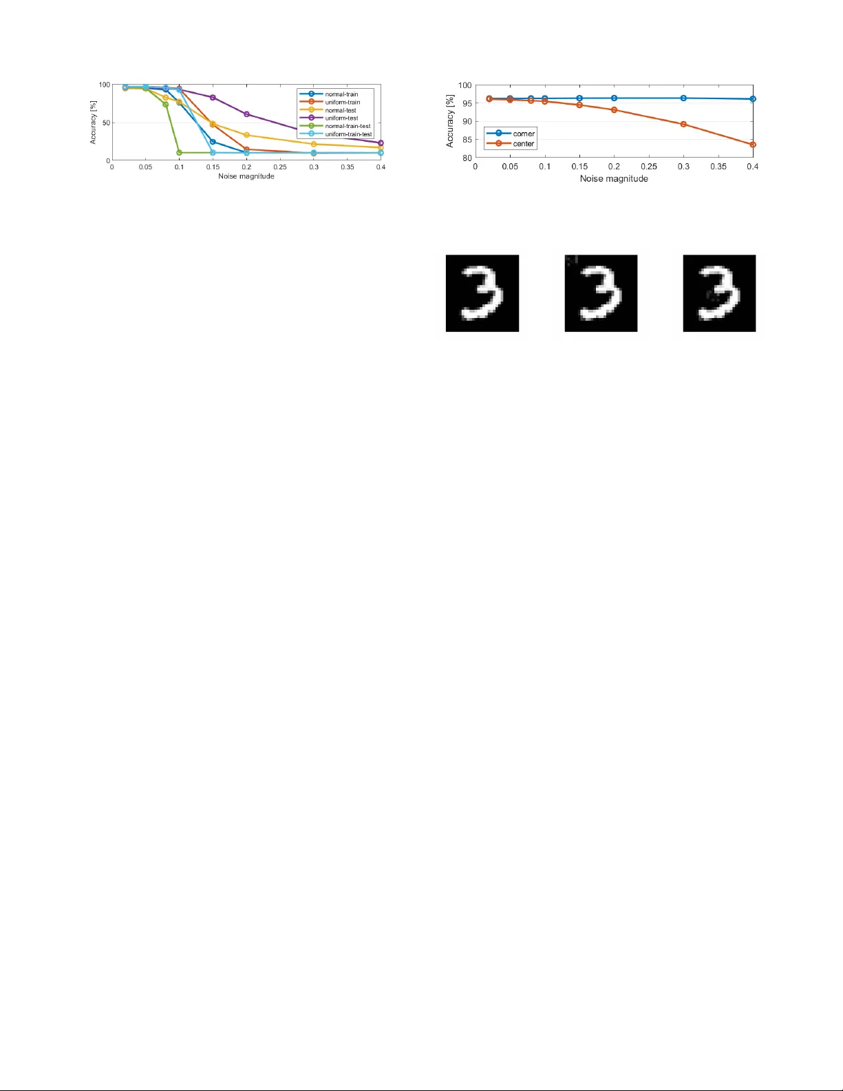
T o appear at the 2020 International Joint Conference on Neural Networks (IJCNN), Glasgo w , Scotland, July 2020. Is Spiking Secure? A Comparati ve Study on the Security V ulnerabilities of Spiking and Deep Neural Networks Alberto Marchisio 1 , Giorgio Nanfa 1 , 2 , Faiq Khalid 1 , Muhammad Abdullah Hanif 1 , Maurizio Martina 2 , Muhammad Shafique 1 1 T ec hnische Universit ¨ at W ien, V ienna, A ustria 2 P olitecnico di T orino, T urin, Italy Email: { alberto.marchisio, faiq.khalid, muhammad.hanif, muhammad.shafique } @tuwien.ac.at giorgio.nanf a@studenti.polito.it, maurizio.martina@polito.it Abstract —Spiking Neural Networks (SNNs) claim to present many advantages in terms of biological plausibility and energy efficiency compared to standard Deep Neural Netw orks (DNNs). Recent works ha ve shown that DNNs ar e vulnerable to adversarial attacks, i.e., small perturbations added to the input data can lead to targeted or random misclassifications. In this paper , we aim at in vestigating the key research question: “Are SNNs secure?” T owards this, we perform a comparative study of the security vulnerabilities in SNNs and DNNs w .r .t. the adversarial noise. Afterwards, we propose a novel black-box attack methodology , i.e., without the knowledge of the internal structure of the SNN, which employs a greedy heuristic to automatically generate imperceptible and r obust adversarial examples (i.e., attack images) for the given SNN. W e perform an in-depth evaluation for a Spiking Deep Belief Network (SDBN) and a DNN having the same number of layers and neurons (to obtain a fair comparison), in order to study the efficiency of our methodology and to understand the differences between SNNs and DNNs w .r .t. the adversarial examples. Our work opens new avenues of research towards the robustness of the SNNs, considering their similarities to the human brain’s functionality . Index T erms —Machine Learning, Neural Networks, Spiking Neural Networks, Security , Adversarial Examples, Attack, V ulnerability , Resilience, SNN, DNN, Deep Neural Network. I . I N T RO D U C T I O N Spiking Neural Networks (SNNs), the third generation neural network models [15], are rapidly emerging as another design option compared to Deep Neural Networks (DNNs), due to their inherent model structure and properties matching the closest to today’ s understanding of a brain’ s functionality . As a result, SNNs hav e the following key properties. • Biologically Plausible : spiking neurons are very similar to the biological ones because they use discrete spikes to compute and transmit information. For this reason, SNNs are also highly sensitiv e to the temporal characteristics of the processed data [5][32]. • Computationally more Powerful than several other NN Models: a lower number of neurons is required to realize/model the same computational functionality [8]. • High Energy Efficiency: spiking neurons process the information only when a new spike arri ves. Therefore, they have relativ ely lower energy consumption compared to complex DNNs, because the spike ev ents are sparse in time [3][21][30]. Such a property makes the SNNs particularly suited for deep learning-based systems where the computations need to be performed at the edge, i.e., in a scenario with limited hardware resources [17]. SNNs ha ve primarily been used for tasks like real- data classification, biomedical applications, odor recognition, navigation and analysis of an en vironment, speech and image recognition [13][25]. Recently , the work of Fatahi et al. [4] proposed to con vert e very pixel of the images into spike trains (i.e., the sequences of spikes) according to its intensity . Since SNNs represent a fundamental step tow ards the idea of creating an architecture as similar as possible to the current understanding of the structure of a human brain, it is fundamental to study their security vulnerability w .r .t. adversarial attacks. In this paper , we demonstrate that indeed, even a small adversarial perturbation of the input images can modify the spike propa gation and incr ease the pr obability of the SNN mispr ediction (i.e., the ima ge is misclassified) . Adversarial Attacks on DNNs: In recent years, many methods to generate adversarial attacks for DNNs and their respectiv e defense techniques have been proposed [7][12][16]. A minimal and imperceptible modification of the input data can cause a classifier misprediction, which can potentially produce a wrong output with high probability . This scenario may lead to serious consequences in safety-critical applications (e.g., automotive, medical, U A Vs and banking) where e ven a single misclassification can have catastrophic consequences [34]. In the image recognition field, ha ving a wide variety of possible real-world input images [12], with di verse pixel intensity patterns, the classifier cannot recognize if the source of the misclassification is the attacker or other factors [26]. 1 Giv en an input image x , the goal of an adv ersarial attack x ∗ = x + δ is to apply a small perturbation δ such that the predicted class C ( x ) is different from the target one C ( x ∗ ) , i.e., the class in which the attacker wants to classify the example. Inputs can also be misclassified without specifying the target class. This is the case of untargeted attacks, where the target class is not defined a-priori by the attacker . T argeted attacks can be more difficult to apply than the untargeted ones, but they can be relati vely more effecti ve in se veral cases [33]. Another important classification of adversarial attacks is based on the kno wledge of the network under attack, as discussed below . • White-box attack: an attacker has the complete access and knowledge of the architecture, the network parameters, the training data and the e xistence of a possible defense. • Black-box attac k: an attacker does not know the architecture, the netw ork parameters, the training data and a possible defense, but it can only access to the input and output of the network (which is treated as a black-box), and may be the testing dataset [24]. Our Appr oach towards Adversarial Attacks on SNNs: In this paper , we aim at generating , for the first time, imper ceptible and r obust adversarial examples for SNNs under the blac k-box settings. Bagheri et al. [1] studied the vulnerabilities of SNNs under white-box assumptions, while we consider a black-box scenario, which makes the attacker stronger under a wide range of real-world scenarios. For the ev aluation, we apply these attacks to a Spiking Deep Belief Network (SDBN) and a DNN ha ving the same number of layers and neurons, to obtain a fair comparison. As per our knowledge 1 , this kind of black-box attack was previously applied only to a DNN model [14]. This method is efficient for DNNs because it is able to generate adversarial noise which is imperceptible to the human eye. As shown in Figure 1, we inv estigate the vulnerability of SDBNs to random noise and adversarial attacks, aiming at identifying the similarities / differences w .r .t. DNNs. Our experiments show that, when applying a random noise to a gi ven SDBN, its classification accurac y decreases, by increasing the noise magnitude. Moreov er , when applying our attack to SDBNs, we observe that, in contrast to the case of DNNs, the output probabilities follo w a dif ferent behavior , i.e., while the adv ersarial image remains imperceptible, the misclassification is not always guaranteed. In short, we make the following Novel Contributions: 1) W e analyze the variation in the accuracy of a Spiking Deep Belief Network (SDBN) when a random noise is added to the input images. ( Section III ) 2) W e ev aluate the improved generalization capabilities of the SDBN when adding a random noise to the training images. ( Section III-C ) 1 A previous v ersion of this work is available in [19]. MNIST Dataset Random adversarial attacks Imperceptible and robust adversarial attacks 9 3 2 7 OUTPUT PROBABILITIES 784 neurons 500 neurons 500 neurons 10 neurons SDBN 4 7 8 6 1 0 5 Fig. 1: Overvie w of our proposed approach. 3) W e de velop a methodology to automatically create imperceptible adversarial e xamples for SNNs. ( Section IV ) 4) W e apply our methodology to an SDBN (it is the first attack of this type applied to SDBNs) and a DNN for generating adversarial examples, and e valuate their imperceptibility and robustness. ( Section V ) Before proceeding to the technical sections, in Section II , we briefly discuss the background and the related work, focusing on SDBNs and adversarial attacks on DNNs. I I . B A C K G RO U N D A N D R E L A T E D W O R K A. Spiking Deep Belief Networks Deep Belief Networks (DBNs) [2] are multi-layer networks that are widely used for classification problems and hav e been implemented in many areas such as visual processing, audio processing, images and text recognition [2]. DBNs are implemented by stacking pre-trained Restricted Boltzmann Machines (RBMs), energy-based models consisting in two layers of neurons, one hidden and one visible, symmetrically and fully connected, i.e., without connections between the neurons inside the same layer (this is the main dif ference w .r .t. the standard Boltzmann machines). RBMs are typically trained with unsupervised learning, to extract the information sav ed in the hidden units, and then a supervised training is performed to train a classifier based on these features [9]. Spiking DBNs (SDBNs) impr ove the energy efficiency and computation speed, as compared to DBNs . Such a behavior has already been observed by O’Connor et al. [23]. That work proposed a DBN model composed of 4 RBMs of 784-500-500-10 neurons, respectively . It has been trained offline and transformed in an event- based domain to increase the processing efficiency and the computational power . The RBMs are trained with the Persistent Contrasti ve Div ergence (CD) algorithm, an unsupervised learning rule using Gibbs sampling, a Markov- Chain Monte-Carlo algorithm, with optimizations for fast weights, selecti vity and sparsity [6][20][31]. Once ev ery RBM is trained, the information is stored in the hidden units to 2 use it as an input for the visible units of the following layer . Afterwards, a supervised learning algorithm [10], based on the features coming from the unsupervised training, is performed. The RBMs of this model use the Sie gert function [28] in their neurons. It allows to have a good approximation of firing rate of Leaky Integrate and Fire (LIF) neurons [5], used for CD training. Hence, the neurons of an SDBN generate Poisson spike trains, according to the Sie gert formula. This represents a great advantage in terms of power consumption and speed, as compared to the classical DBNs, which are based on a discrete-time model [23]. Since ther e has been no prior work on studying the security vulnerabilities of SNNs / SDBNs, we aim at in vestigating these aspects in a black-box setting, which is important for their r eal-world applications in security/safety-critical systems . B. Adversarial Attacks for DNNs The robustness and self-healing properties of DNNs have been thoroughly in vestig ated in the recent researches [27]. As demonstrated for the first time by Szegedy et al. [29], adversarial attacks can misclassify an image by changing its pixels with small perturbations. Kurakin et al. [12] defined adversarial e xamples as a sample of input data which has been modified very slightly in a way that is intended to cause a machine learning classifier to misclassify it . Luo et al. [14] proposed a method to generate attacks by maximizing their noise tolerance and taking into account the human perceptual system in their distance metric. A similar attack is able to mislead even more complex DNNs, like Capsule Networks [18], which are notoriously more robust against adversarial attacks. This methodology has strongly inspired our algorithm. The human eyes are more sensiti ve to the modifications of the pixels in low variance areas. Hence, to maintain the imperceptibility as much as possible, the modification of pixels in only the high variance areas is preferable. Moreov er , a robust attack aims at increasing its ability to stay misclassified to the tar get class after the transformations due to the physical world . For example, considering a crafted sample, after an image compression or a resizing, its output probabilities can change according to the types of the applied transformations. Therefore, the attack can be ineffecti v e if it is not robust enough to those variations. Motiv ated by the above-discussed considerations, we pr opose an algorithm to automatically generate imper ceptible and r ob ust adversarial examples for SNNs, and study their differ ences w .r .t. the adversarial examples generated for DNNs using the same technique . I I I . A NA LY S I S : A P P L Y I N G R A N D O M N O I S E T O S D B N S A. Experimental Setup For a case study , we consider an SDBN [23] composed of four fully-connected layers of 784-500-500-10 neurons, respectiv ely . W e implement this SDBN in Matlab, for analyzing the MNIST database, a collection of 28 × 28 gray scale images of handwritten digits, di vided into 60,000 training images and 10,000 test images. Each pixel intensity is encoded as a value between 0 and 255. T o maximize the spike firing, the input data are scaled to the range [0,0.2], before con verting them into spikes. In our experiments, the pixel intensities are represented as the probability that a spike occurs. B. Understanding the Impact of Random Noise Addition to Inputs on the Accuracy of an SDBN W e test the accuracy of the SDBN for different noise magnitudes, applied to three different combinations of images: • to all the training images only . • to all the test images only . • to both the training and test images. T o test the vulnerability of the SDBN, we apply two different types of noises: normally-distributed and uniformly- distributed random noise. The results of our experiments are shown in T able I and Figure 2. The initial “clean-case” accuracy , obtained without applying noise, is 96 . 2% . When the noise is applied to the test images, the accuracy of the SDBN decreases accordingly with an increase in the noise magnitude, more evidently in the case of the normally-distributed random noise. This behavior is due to the fact that the standard normal distribution contains a wider range of values, compared to the uniform distribution. For both noise distributions, the accurac y decreases more when the noise magnitude applied is around 0.15 (see the red- colored values in T able I). T ABLE I: Evaluation of the SDBN accuracy applying two different types of random noise with different values of noise magnitude. The red and blue values are helping the reader to identify the accuracy results that are discussed in the text. (A CC stands for Accuracy , TR+TST stands for Training and T est Datasets) A CC TRAIN TEST TR+TST TRAIN TEST TR+TST δ NORMALL Y UNIFORML Y 0.02 96.65 94.73 96.54 96.8 96.02 96.81 0.05 95.19 94.42 94.99 96.7 95.64 96.72 0.08 92.99 82.73 73.64 95.89 94.64 95.56 0.1 76.01 77.07 10.39 94.34 93.36 92.8 0.15 24.61 48.23 10.32 47.03 82.76 10.51 0.2 10.26 33.34 10.05 14.64 60.79 10.16 0.3 10.31 21.52 9.88 9.59 34.9 10.16 0.4 10.27 17.05 10.34 9.98 23.16 10.03 When the noise is applied to the training images, the accuracy of the SDBN does not decrease as much as in the previous case, as long as the noise magnitude ( δ ) is lower than 0.1. On the contrary , for δ = 0 . 02 , the accuracy increases (see the blue-colored v alues in T able I) w .r .t. the baseline (i.e., without noise). Indeed, adding noise in training samples improves the generalization capabilities of the neural network. Hence, its capability to correctly classify new unseen 3 Fig. 2: Normal and uniform random noise applied to all the pixels of the MNIST dataset. samples also increases. This observ ation, as was analyzed in sev eral other scenarios for Deep Neural Networks with back- propagation training [11], is also valid for our SDBN model. Howe v er , if the noise is equal to or greater than 0.1, the accuracy drops significantly . This behavior means that the SDBN is unable to learn input features due to the inserted noise, thus it is unable to correctly classify the inputs. When the noise is applied to both the training and test images, we notice that the behavior observed for the case of noise applied to only the training images is accentuated. For low noise magnitudes (mostly in the uniform noise case), the accuracy is similar or higher than the baseline. For noise magnitudes greater than 0.1 (more precisely , 0.08 for the case of normal noise applied), the accuracy decreases more sharply than in the case of noise applied only to the training images. Such a value of noise magnitude represents a threshold of tolerable noise for the SDBN. Hence, when the noise is too high, the network cannot classify well. C. Applying Noise to a Restricted W indow of Pixels In this analysis, we add a normally distributed random noise to a restricted windo w of pix els of the test images. Considering a rectangle of 4 × 5 pixels, we analyze two scenarios: • The noise is applied to 20 pixels at the top-left corner of the image. The variation of the accuracy is represented by the blue-colored line of Figure 3. As expected, the accuracy remains almost constant, because the noise affects irrelev ant pixels. The resulting image, when the noise is equal to 0.3, is shown in Figure 4b. • The noise is applied to 20 pixels in the middle of the image, with coordinates ( x, y ) = ([14 17] , [10 14]) . The accuracy descreases more significantly (orange- colored line of Figure 3), as compared to the previous case, because some white pixels representing the handwritten digits (and therefore the important ones for the classification) are af fected by the noise. The resulting image, when the noise is equal to 0.3, is sho wn in Figure 4c. This analysis shows that the location of noise insertion impacts the accuracy , thereby unleashing a potential vulnerability of SNNs that can be exploited by the adversarial attacks. D. Ke y Observations fr om our Analyses From the analyses performed in the above Sections III-B and III-C, we deriv e the following k ey observ ations that can be Fig. 3: Normal random noise applied to some pixels of the MNIST test images. (a) (b) (c) Fig. 4: Comparison between images with normally distributed random noise (with magnitude 0.3) applied to the corner and to the left center of the image. (a) Without noise. (b) Noise applied to the top-left corner . (c) Noise applied to the center . exploited by an adv ersarial example generation methodology . • The normal noise is more powerful than the uniform counterpart, since the accuracy decreases more sharply . • For a low noise magnitude applied to the training images, we notice a small accuracy improv ement, due to the improv ed generalization capability of SDBNs. • When applying the noise to a restricted window of pixels, the perturbation is more effecti ve if the windo w is in the center of the image (or generally speaking, in the input regions belonging to the features that are key for the correct classification), as compared to the corner . This is due to the fact that the noise is applied to the pixels which play an important role for accurate feature learning and consequently for the correct classification. I V . O U R N O V E L M E T H O D O L O G Y T O G E N E R AT E I M P E R C E P T I B L E A N D R O B U S T A DV E R S A R I A L E X A M P L E S Similar to the case of DNNs, the scope of a good attack on SNNs is also to generate adversarial images, which ar e difficult to be detected by human e yes (i.e., imper ceptible) and r esistant to physical transformations (i.e., rob ust) . Therefore, for better understanding, we first discuss these two aspects. A. Imperceptibility of Adversarial Examples Creating an imperceptible example means to add perturbations to the pixels, while making sure that humans do not notice them. W e consider an area A=N · N of pixels x , 4 and we compute the standard deviation (SD) of a pixel x i,j as in Equation (1). S D ( x i,j ) = v u u u t N P k =1 N P l =1 ( x k,l − µ ) 2 − ( x i,j − µ ) 2 N · N (1) Here, µ is the av erage v alue of pixels belonging to the N · N area. If a pixel has a high standard de viation, it means that a perturbation added to this pixel is more likely to be hardly detected by the human eye, compared to a pixel with a low standard de viation. The sum of all the perturbations δ added to the pixels of the area A allows to compute the distance ( D ( X ∗ , X ) ) between the adversarial example X ∗ and the original one X . Its formula is shown in Equation (2). D ( X ∗ , X ) = N X i =1 N X j =1 δ i,j S D ( x i,j ) (2) Such value can be used to monitor the imperceptibility . Indeed, the distance D ( X ∗ , X ) indicates ho w much perturbation is added to the pixels in the area A. Hence, the maximum perturbation tolerated by the human e ye can be associated to a certain value of the distance, D M AX . The value of D M AX can vary among dif ferent datasets or images, because it depends on the resolution and the contrast between neighboring pixels. B. Robustness of adversarial e xamples Many adversarial attack methods used to maximize the probability of target class to ease the classifier misclassification of the image. The main problem of these methods is that the y do not account for the relativ e difference between the class probabilities, i.e., the gap, defined in Equation (3). Gap ( X ∗ ) = P ( tar get cl ass ) − max { P ( other cl asses ) } (3) Therefore, after an image transformation, a minimal modification of the probabilities can make the attack ineffecti v e. T o improv e the robustness, it is desirable to increase the difference between the probability of the target class and the highest probability of the other classes, i.e., to maximize the gap function. C. How to Automatically Generate Attac ks for SNNs? Obtaining both the imperceptibility and robustness at the same time is complicated. T ypically , a robust attack would require perceptible changes of the input, while an imperceptible attack does not change the classification much. W e designed a heuristic algorithm to automatically generate imperceptible yet rob ust adversarial examples for SNNs. Our technique is also applicable to DNNs, as we will demonstrate in the result section. Note that, leveraging the same methodology to generate adversarial examples for both SNNs and DNNs enables a fair comparison. Our algorithm is based on the black-box model, i.e., the attacks are performed on some pixels of the image, without having insights of the network. Gi ven the maximum allowed distance D M AX such that human eyes cannot detect perturbations, the problem can be expressed as in Equation (4). arg max X ∗ Gap ( X ∗ ) | D ( X ∗ , X ) ≤ D M AX (4) In summary , the purpose of our iterative algorithm is to perturb a set of pixels, to maximize the gap function, thus making the attac k r ob ust, while keeping the distance between the samples below the desired thr eshold, in or der to r emain imper ceptible . Based on the key observations of our analysis in Section III-D, our iterati ve methodology (see Algorithm 1) perturbs only a window of pixels of the image. W e choose a certain value N, which corresponds to an area of N · N pixels, performing the attack on a subset M of pixels. Algorithm 1 : Methodology for Generating Adversarial Examples for SNNs and DNNs Giv en: network (SNN or DNN), original sample X, maximum human perceptual distance D max , noise magnitude δ , area of A pixels, target class, M while D ( X ∗ , X ) < D M AX do -Compute Standar d Deviation SD for every pixel of A -Compute Gap ( X ∗ ) , Gap − ( X ∗ ) , Gap + ( X ∗ ) if Gap ( X ∗ ) − > Gap ( X ∗ ) + then V ariationP r iority ( x i,j ) = [ Gap − ( X ∗ ) − Gap ( X ∗ )] · S D ( x i,j ) else V ariationP r iority ( x i,j ) = [ Gap + ( X ∗ ) − Gap ( X ∗ )] · S D ( x i,j ) end if -Sort in descending order V ar iationP r iority -Select M pixels with highest V ar iationP r iority if Gap ( X ∗ ) − > Gap ( X ∗ ) + then Subtract noise with magnitude δ from the pix el else Add noise with magnitude δ to the pix el end if -Compute D ( X ∗ , X ) -Update the original example with the adv ersarial one end while After computing the standard deviation for the selected N · N pixels, we compute the gap function, i.e., the difference between the probability of the tar get class and the highest probability between the other classes. Then, the algorithm decides whether to apply a positiv e or a negati ve noise to the pixels. Therefore, we compute two parameters for each pixel, Gap + ( X ∗ ) and Gap − ( X ∗ ) . Gap + ( X ∗ ) is the value of the gap function computed by adding a perturbation unit to the single pixel, while Gap − ( X ∗ ) is its counterpart, computed subtracting a perturbation unit. According to the 5 X* 784 NEURONS 500 NEURONS 10 NEURONS 500 NEURONS 3 5 V ARIA TION PRIORITY PIXELS SELECTION D(X*,X) D(X*,X)