PLLay: Efficient Topological Layer based on Persistence Landscapes

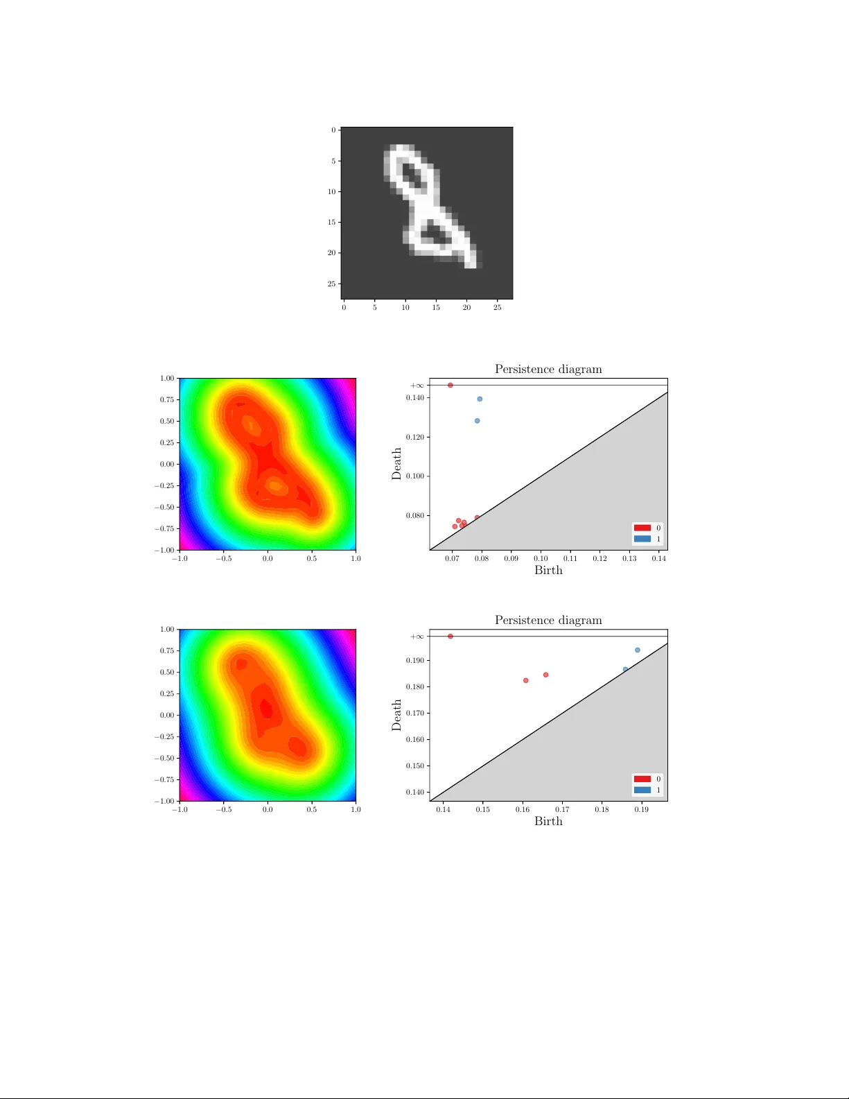
PLLay: Efﬁcient T opological Layer based on P ersistence Landscapes Kwangho Kim Carnegie Mellon Uni versity Pittsbur gh, USA kwanghk@cmu.edu Jisu Kim Inria Palaiseau, France jisu.kim@inria.fr Manzil Zaheer Google Research Mountain V iew , USA manzilzaheer@google.com Joon Sik Kim Carnegie Mellon Uni versity Pittsbur gh, USA joonsikk@cs.cmu.edu Frederic Chazal Inria Palaiseau, France frederic.chazal@inria.fr Larry W asserman Carnegie Mellon Uni versity Pittsbur gh, USA larry@stat.cmu.edu Abstract W e propose PLLay , a nov el topological layer for general deep learning models based on persistence landscapes, in which we can ef ﬁciently exploit the underlying topological features of the input data structure. In this work, we sho w differentia- bility with respect to layer inputs, for a general persistent homology with arbitrary ﬁltration. Thus, our proposed layer can be placed anywhere in the network and feed critical information on the topological features of input data into subsequent layers to improv e the learnability of the networks toward a given task. A task- optimal structure of PLLay is learned during training via backpropagation, without requiring any input featurization or data preprocessing. W e provide a novel adap- tation for the DTM function-based ﬁltration, and sho w that the proposed layer is robust ag ainst noise and outliers through a stability analysis. W e demonstrate the effecti veness of our approach by classiﬁcation experiments on v arious datasets. 1 Introduction W ith its strong generalizability , deep learning has been pervasi vely applied in machine learning. T o improv e the learnability of deep learning models, various techniques have been proposed. Some of them hav e achieved an ef ﬁcient data processing method through specialized layer structures; for instance, inserting a con volutional layer greatly improv es visual object recognition and other tasks in computer vision [e.g., Krizhe vsky et al., 2012, LeCun et al., 2016]. On the other hand, a large body of recent work focuses on optimal architecture of deep network [Simonyan and Zisserman, 2015, He et al., 2016, Szegedy et al., 2015, Albelwi and Mahmood, 2016]. In this paper , we explore an alternati ve way to enhance the learnability of deep learning models by de veloping a nov el topological layer which feeds the signiﬁcant topological features of the underlying data structure in an arbitrary network. The power of topology lies in its capacity which differentiates sets in topological spaces in a robust and meaningful geometric way [Carlsson, 2009, Ghrist, 2008]. It provides important insights into the global "shape" of the data structure via persistent homology Preprint. Figure 1: Illustration of PLLay , a nov el topological layer based on weighted persistence landscapes. Information in the persistence diagram is ﬁrst encoded into persistence landscapes as a form of vectorized function, and then a deep learning model determines which components of the landscape (e.g., particular hills or v alleys) are important for a gi ven task during training. PLLay can be placed anywhere in the network. [Zomorodian and Carlsson, 2005]. The use of topological methods in data analysis has been limited by the dif ﬁculty of combining the main tool of the subject, persistent homology, with statistics and machine learning. Nonetheless, a series of recent studies have reported notable successes in utilizing topological methods in data analysis [e.g., Zhu, 2013, Dindin et al., 2020, Nanda and Sazdanovi ´ c, 2014, T ralie and Perea, 2018, Sev ersky et al., 2016, Gamble and Heo, 2010, Pereira and de Mello, 2015, Umeda, 2017, Liu et al., 2016, V enkataraman et al., 2016, Emrani et al., 2014] There are at least three beneﬁts of utilizing the topological layer in deep learning; 1) we can ef ﬁciently extract robust global features of input data that otherwise would not be readily accessible via traditional feature maps, 2) an optimal structure of the layer for a giv en task can be easily embodied via backpropagation during training, and 3) with proper ﬁltrations it can be applied to arbitrarily complicated data structure ev en without any data preprocessing. Related W ork. The idea of incorporating topological concepts into deep learning has been explored only recently , mostly via feature engineering perspectiv e where we use some ﬁx ed, predeﬁned features that contain topological information [e.g., Dindin et al., 2020, Umeda, 2017, Liu et al., 2016]. Guss and Salakhutdinov [2018], Rieck et al. [2019] proposed a complexity measure for neural network architectures based on topological data analysis. Carlsson and Gabrielsson [2020] applied topological approaches to deep con volutional networks to understand and improv e the computations of the network. Hofer et al. [2017] ﬁrst developed a technique to input persistence diagrams into neural networks by introducing their o wn topological layer . Carrière et al. [2020] proposed a network layer for persistence diagrams built on top of graphs. Poulenard et al. [2018], Gabrielsson et al. [2019], Hofer et al. [2019], Moor et al. [2020] also proposed various topology loss functions and layers applied to deep learning. Nev ertheless, all the previous approaches suf fer from at least one or more of the following limitations: 1) they rely on a particular parametrized map or ﬁltration, 2) they lack stability results or the stability is limited to a particular type of input data representation, and 3) most importantly , the differentiability of persistent homology is not guaranteed with respect to the layer’ s input therefore we can not place the layer in the middle of deep networks in general. Contribution. This paper presents a new topological layer, PLLay (Persistence Landscape-based topological Layer: see Figure 1 for an illustration), that does not suf fer from the abov e limitations. Our topological layer does not rely on a particular ﬁltration or a parametrized mapping b ut still sho ws fa vorable theoretical properties. The proposed layer is designed based on the weighted persistence landscapes to be less prone to extreme topological distortions. W e provide a tight stability bound that does not depend on the input comple xity , and sho w the stability with respect to input perturbations. W e also provide a no vel adaptation for the DTM function-based ﬁltration, and analyze the stability property . Importantly , we guarantee the differentiability of our layer with respect to the layer’ s input. Reproducibility . The code for PLLay is av ailable at https://github.com/jisuk1/pllay/ . 2 2 Background and deﬁnitions T opological data analysis (TD A) is a recent and emer ging ﬁeld of data science that relies on topo- logical tools to infer relev ant features for possibly complex data [Carlsson, 2009]. In this section, we brieﬂy revie w basic concepts and main tools in TDA which we will harness to de velop our topological layer in this paper . W e refer interested readers to Chazal and Michel [2017], Hatcher [2002], Edelsbrunner and Harer [2010], Chazal et al. [2009, 2016b] for details and formal deﬁnitions. 2.1 Simplicial complex, persistent homology , and diagrams When inferring topological properties of X , a subset of R d , from a ﬁnite collection of samples X , we rely on a simplicial complex K , a discrete structure built ov er the observed points to provide a topological approximation of the underlying space. T wo common examples are the ˇ Cech complex and the V ietoris-Rips complex. The ˇ Cech comple x is the simplicial complex where k -simplices correspond to the nonempty intersection of k + 1 balls centered at vertices. The V ietoris-Rips (or simply Rips ) comple x is the simplicial comple x where simple xes are built based on pairwise distances among its vertices. W e refer to Appendix A for formal deﬁnitions. A collection of simplicial complexes F = { K a ⊂ K : a ∈ R } satisfying K a ⊂ K b whenev er a ≤ b is called a ﬁltration of K . A typical way of setting the ﬁltration is through a monotonic function on the simplex. A function f : K → R is monotonic if f ( ς ) ≤ f ( τ ) whenev er ς is a face of τ . If we let K a : = f − 1 ( −∞ , a ] , then the monotonicity implies that K a is a subcomplex of K and K a ⊂ K b whenev er a ≤ b . In this paper, we assume that the ﬁltration is b uilt upon a monotonic function. P ersistent homology is a multiscale approach to represent the topological features of the complex K , and can be represented in the persistence diagram. For a ﬁltration F and for each nonnegati ve k , we keep track of when k -dimensional homological features (e.g., 0 -dimension: connected component, 1 -dimension: loop, 2 -dimension: cavity , . . . ) appear and disappear in the ﬁltration. If a homological feature α i appears at b i and disappears at d i , then we say α i is born at b i and dies at d i . By considering these pairs ( b i , d i ) as points in the plane, one obtains the persistence diagr am deﬁned as follows. Deﬁnition 2.1 Let R 2 ∗ : = { ( b, d ) ∈ ( R ∪ ∞ ) 2 : d > b } . A persistence diagram D is a ﬁnite multiset of { p : p ∈ R 2 ∗ } . W e let D denote the set of all such D ’ s. W e will use D X , D X as shorthand notations for the persistence diagram drawn from the simplicial complex constructed on original data source X, X , respectiv ely . Lastly , we deﬁne the following metrics to measure the distance between two persistence diagrams. Deﬁnition 2.2 (Bottleneck and W asserstein distance) Given two persistence dia grams D and D 0 , their bottleneck distance ( d B ) and q -th W asserstein distance ( W q ) for q ≥ 1 ar e deﬁned by d B ( D , D 0 ) = inf γ ∈ Γ sup p ∈ ¯ D k p − γ ( p ) k ∞ , W q ( D , D 0 ) = " inf γ ∈ Γ X p ∈ ¯ D k p − γ ( p ) k q ∞ # 1 q , (1) r espectively , wher e k · k ∞ is the usual L ∞ -norm, ¯ D = D ∪ Diag and ¯ D 0 = D 0 ∪ Diag with Diag being the diagonal { ( x, x ) : x ∈ R } ⊂ R 2 with inﬁnite multiplicity , and the set Γ consists of all the bijections γ : ¯ D → ¯ D 0 . Note that for all q ∈ [1 , ∞ ) , d B ( D X , D Y ) ≤ W q ( D X , D Y ) for any giv en D X , D Y . As q tends to inﬁnity , the W asserstein distance approaches the bottleneck distance. Also, see Appendix B for a further relationship between the bottleneck distance and W asserstein distance. 2.2 Persistence landscapes A persistence diagram is a multiset, which is difﬁcult to be used as inputs for machine learning methods (due to the complicated space structure, cardinality issues, computationally inef ﬁcient metrics, etc.). Hence, it is useful to transform the persistent homology into a functional Hilbert space, where the analysis is easier and learning methods can be directly applied. One good example is the persistence landscape [Bubenik, 2015, 2018, Bubenik and Dłotko, 2017]. Let D denote a persistence 3 diagram that contains N off-diagonal birth-deat h pairs. W e ﬁrst consider a set of piece wise-linear functions { Λ p ( t ) } p ∈D for all birth-death pairs p = ( b, d ) ∈ D as Λ p ( t ) = max { 0 , min { t − b, d − t }} . Then the persistence landscape λ of the persistence diagram D is deﬁned as a sequence of functions { λ k } k ∈ N , where λ k ( t ) = kmax p Λ p ( t ) , t ∈ R , k ∈ N , (2) Hence, the persistence landscape is a set of real-valued functions and is easily computable. Advantages for this kind of functional summaries are discussed in Chazal et al. [2014b], Berry et al. [2018]. 2.3 Distance to measure (DTM) function The Distance to measure (DTM) [Chazal et al., 2011, 2016a] is a robustiﬁed version of the distance function. More precisely , the DTM d µ,m 0 : R d → R for a probability distrib ution µ with parameter m 0 ∈ (0 , 1) and r ≥ 1 is deﬁned by d µ,m 0 ( x ) =  1 m 0 Z m 0 0 ( δ µ,m ( x )) r dm  1 /r , where δ µ,m ( x ) = inf { t > 0 : µ ( B ( x, t )) > m } when B ( x, t ) is an open ball centered at x with radius t . If not speciﬁed, r = 2 is used as a default. In practice, we use a weighted empirical measure P n ( x ) = P n i =1 $ i 1 ( X i = x ) P n i =1 $ i , with weights $ i ’ s for µ . In this case, we deﬁne the empirical DTM by ˆ d m 0 ( x ) = d P n ,m 0 ( x ) = P X i ∈ N k ( x ) $ 0 i k X i − x k r m 0 P n i =1 $ i ! 1 /r , (3) where N k ( x ) is the subset of { X 1 , . . . , X n } containing the k nearest neighbors of x , k is such that P X i ∈ N k − 1 ( x ) $ i < m 0 P n i =1 $ i ≤ P X i ∈ N k ( x ) $ i , and $ 0 i = P X j ∈ N k ( x ) $ j − m 0 P n j =1 $ j if at least one of X i ’ s is in N k ( x ) and $ 0 i = $ i otherwise. Hence the empirical DTM behav es similarly to the k -nearest distance with k = b m 0 n c . For i.i.d cases, we typically set $ i = 1 but the weights can be ﬂexibly determined in data-driv en way . The parameter m 0 determines how much topological/geometrical information should be extracted from the local or global structure. A brief guideline on DTM parameter selection can be found in Appendix F (see Chazal et al. [2011] for more details). Since the resulting persistence diagram is less prone to input perturbations and has nice stability properties, people often prefer using the DTM as their ﬁltration function. 3 A novel topological lay er based on weighted persistence landscapes In this section, we present a detailed algorithm to implement PLLay for a general neural network. Let X , D X , h top denote our input, corresponding persistence diagram induced from X , the proposed topological layer , respectively . Broadly speaking, the construction of our proposed topological layer consists of two steps: 1) computing a persistence diagram from the input, and 2) constructing the topological layer from the persistence diagram. 3.1 Computation of diagram: X → D X T o compute the persistence diagram from the input data, we ﬁrst need to deﬁne the ﬁltration which requires a simplicial complex K and a function f : K → R . There are sev eral options for K and f . W e are in general agnostic about which ﬁltration to use since it is in fact problem-dependent; in practice, we suggest using ensemble-like methods that can adapt to v arious underlying topological structures. One popular choice is the V ietoris-Rips ﬁltration. When there is a one-to-one correspon- dence between X i and each ﬁxed grid point Y i , one obvious choice for f could be just interpreting X as a function values, so f ( Y i ) = X i . W e refer to Chazal and Michel [2017] for more examples. As described in Section 2.3, one appealing choice for f is the DTM function. Due to its fa vorable properties, the DTM function has been widely used in TD A [Anai et al., 2019, Xu et al., 2019], and 4 Figure 2: The topological features encoded in the persis- tence diagram & persistence landscapes for MNIST and ORBIT5k sample. In the MNIST example, two loops (1-dimensional feature) in ‘ 8 ’ are clearly identiﬁed and en- coded into the 1st and 2nd order landscapes. The ORBIT5k sample shows more in volved patterns. Figure 3: The signiﬁcant point (inside green-dashed circle) in the persistence diagram remains almost unchanged e ven after corrupting pixels and adding noise to the image. has a good potential for deep learning application. Nonetheless, to the best of our knowledge, the DTM function has not yet been adopted in previous studies. In what follows, we detail two common scenarios for the DTM adaptation: when we consider the input X as 1) data points or 2) weights. • If the input data X is considered as the empiri- cal data points, then the empirical DTM in (3) with weights $ i ’ s becomes ˆ d m 0 ( x ) = P X i ∈ N k ( x ) $ 0 i k X i − x k r m 0 P n i =1 $ i ! 1 /r , (4) where k and $ 0 i are determined as in (3). • If the input data X is considered as the weights corresponding to ﬁxed points { Y 1 , . . . , Y n } , then the empirical DTM in (3) with data points Y i ’ s and weights X i ’ s becomes ˆ d m 0 ( x ) = P X i ∈ N k ( x ) X 0 i k Y i − x k r m 0 P n i =1 X i ! 1 /r , (5) where k and $ 0 i are determined as in (3). Figure 2 provides some real data examples (which will be used in Section 5) of the persistence diagrams and the corresponding persistence landscapes based on the DTM functions. As shown in Figure 3, the topological features are expected to be rob ust to external noise or corruption. 3.2 Construction of topological layer: D X → h top Our topological layer is deﬁned based on a parametrized mapping which takes the persistence diagram D to be projected onto R , by harnessing persistence landscapes. Our construction is less afﬂicted by the artiﬁcial bending due to a particular transformation procedure as in Hofer et al. [2017], yet still guarantees the crucial information in the persistence diagram to be well preserved as will be seen in Section 4. Insigniﬁcant points with low persistence are lik ely to be ignored systematically without introducing additional nuisance parameters [Bubenik and Dłotko, 2017]. Let R +0 denote [0 , ∞ ) . Gi ven a persistence diagram D ∈ D , we compute the persistence landscape of order k in (2) , λ k ( t ) , for k = 1 , ..., K max . Then, we compute the weighted av erage λ ω ( t ) : = P K max k =1 ω k λ k ( t ) with a weight parameter ω = { ω k } k , ω k > 0 , P k ω k = 1 . Next, we set a domain [ T min , T max ] and a resolution ν : = T / ( m − 1) , and sample m equal-interv al points from [ T min , T max ] to obtain Λ ω =  λ ω ( T min ) , λ ω ( T min + ν ) , ..., λ ω ( T max )  > ∈  R +0  m . Consequently , we hav e deﬁned a mapping Λ ω : D →  R +0  m which is a (vectorized) ﬁnite-sample approximation of the weighted persistence landscapes at the resolution ν , at ﬁxed, predetermined locations. Finally , we consider a parametrized differentiable map g θ :  R +0  m → R which takes the input Λ ω and is differentiable with respect to θ as well. Now , the projection of D with respect to the mapping 5 Algorithm 1 Implementation of single structure element for PLLay Input: persistence diagram D ∈ D 1. compute λ k ( t ) (2) on t ∈ [0 , T ] for e very k = 1 , ..., K max 2. compute the weighted average λ ω ( t ) : = P K max k =1 ω k λ k ( t ) , ω k > 0 , P k ω k = 1 3. set ν : = T m − 1 , and compute Λ ω = ( λ ω ( T min ) , λ ω ( T min + ν ) , ..., λ ω ( T max )) > ∈ R m 4. for a parametrized differentiable map g θ : R m → R , deﬁne S θ , ω = g θ ◦ Λ ω Output: S θ , ω : D → R S θ , ω : = g θ ◦ Λ ω deﬁnes a single structur e element for our topological input layer . W e summarize the procedure in Algorithm 1. The projection S θ , ω is continuous at ev ery t ∈ [ T min , T max ] . Also, note that it is dif ferentiable with respect to ω and θ , regardless of the resolution le vel ν . In what follows, we provide some guidelines that might be useful to implement Algorithm 1. ω : The weight parameter ω can be initialized uniformly , i.e. ω k = 1 /K max for all k , and will be re-determined during training through the softmax layer in a way that a certain landscape conv ey- ing signiﬁcant information has more weight. In general, lower -order landscapes tend to be more signiﬁcant than higher-order landscapes, b ut the optimal weights may vary from task to task. θ , g θ : Like wise, some birth-death pairs, encoded in the landscape function, may contain more crucial information about the topological features of the input data structure than others. Roughly speaking, this is equi valent to say certain mountains (or their ridge or v alley) in the landscape are especially important. Hence, the parametrized map g θ should be able to reﬂect this by its design. In general, it can be done by afﬁne transformation with scale and translation parameter, follo wed by an extra nonlinearity and normalization if necessary . W e list two possible choices as belo w . • Afﬁne transformation: with scale and translation parameter σ i , µ i ∈ R m , g θ i ( Λ ω ) = σ > i ( Λ ω − µ i ) and θ i = ( σ i , µ i ) . • Logarithmic transformation: with same θ i = ( σ i , µ i ) , g θ i ( Λ ω ) = exp  − σ i k Λ ω − µ i k 2  . Note that other constructions of g θ , θ , ω are also possible as long as they satisfy the sufﬁcient conditions described abov e. Finally , since each structure element corresponds to a single node in a layer , we concatenate many of them, each with different parameters, to form our topological layer . Deﬁnition 3.1 (Persistence landscape-based topological lay er ( PLLay )) F or n h ∈ N , let η i = ( θ i , ω i ) denote the set of parameters for the i -th structure element and let η = ( η i ) n h i =1 . Given D and r esolution ν , we deﬁne PLLay as a parametrized mapping with η of D → R n h such that h top : D →  S η i ( D ; ν )  n h i =1 . (6) Note that this is nothing but a concatenation of n h topological structure elements (nodes) with different parameter sets (thus n h is our layer dimension). Remark 1 Our PLLay considers only K max top landscape functions. F or a given persistence diagram, the points near the diagonal ar e not likely to appear at K max top landscape functions, and hence not consider ed in PLLay . And hence PLLay automatically ﬁlters out the noisy featur es. 3.3 Differentiability This subsection is dev oted to the analysis of the dif ferential beha vior of PLLay with respect to its input (or output from the pre vious layer), by computing the deri vati ves ∂ h top ∂ X . Since ∂ h top ∂ X = ∂ h top ∂ D X ◦ ∂ D X ∂ X , this can be done by combining two deriv atives ∂ D X ∂ X and ∂ h top ∂ D X . W e hav e extended Poulenard et al. [2018] so that we can compute the above deri vati ves for general persistent homology under arbitrary ﬁltration in our setting. W e present the result in Theorem 3.1. 6 Theorem 3.1 Let f be the ﬁltration function. Let ξ be a map fr om each birth-death point ( b i , d i ) ∈ D X to a pair of simplices ( β i , δ i ) . Suppose that ξ is locally constant at X , and f ( β i ) and f ( δ i ) ar e differ entiable with r espect to X j ’ s. Then, h top is differ entiable with r espect to X and ∂ h top ∂ X j = X i ∂ f ( β i ) ∂ X j m X l =1 ∂ g θ ∂ x l K max X k =1 ω k ∂ λ k ( lv ) ∂ b i + X i ∂ f ( δ i ) ∂ X j m X l =1 ∂ g θ ∂ x l K max X k =1 ω k ∂ λ k ( lv ) ∂ d i . The proof is in Appendix E.1. Note that ∂ λ k ∂ b i , ∂ λ k ∂ d i are piecewise constant and are easily computed in explicit forms. Also ∂ g θ ∂ x l can be easily realized by an automatic diff erentiation framew ork such as tensorflow or pytorch . Our PLLay in Deﬁnition 3.1 is thus trainable via backpropagation at an arbitrary location in the network. In Appendix D, we also provide a deri vati ve for the DTM ﬁltration. 4 Stability Analysis A key property of PLLay is stability; its discriminating power should remain stable against non- systematic noise or perturbation of input data. In this section, we shall provide our theoretical results on the stability properties of the proposed layer . W e ﬁrst address the stability for each structure element with respect to changes in persistence diagrams in Theorem 4.1. Theorem 4.1 Let g θ be k · k ∞ -Lipschitz, i.e. ther e e xists L g > 0 with | g θ ( x ) − g θ ( y ) | ≤ L g k x − y k ∞ for all x, y ∈ R m . Then for two persistence diagr ams D , D 0 , | S θ , ω ( D ; ν ) − S θ , ω ( D 0 ; ν ) | ≤ L g d B ( D , D 0 ) . Proof of Theorem 4.1 is giv en in Appendix E.2. Theorem 4.1 sho ws that S θ , ω is stable with respect to perturbations in the persistence diagram measured by the bottleneck distance (1) . It should be noted that only the Lipschitz continuity of g θ is required to establish the result. Next, Corollary 4.1 sho ws that under certain conditions our approach improves the pre vious stability result of Hofer et al. [2017]. Corollary 4.1 F or t > 0 , let n t ∈ N be satisfying that, for any two diagrams D t , D 0 t with d B ( D , D t ) ≤ t and d B ( D 0 , D 0 t ) ≤ t , either D t \D 0 t or D 0 t \D t has at least n t points. Then, the ratio of our stability bound in Theor em 4.1 to that in Hofer et al. [2017] is upper bounded by C g θ / (1 + (2 t/d B ( D , D 0 )) × ( n t − 1)) , wher e C g θ is a constant to be speciﬁed in the pr oof. See Appendix E.3 for the proof. Corollary 4.1 implies that for complex data structures where each D contains many birth-death pairs (for ﬁx ed t , in general n t grows with the increase in the number of points in D ), our stability bound is tighter than that of Hofer et al. [2017] at polynomial rates. In particular , when we use the DTM function-based ﬁltration proposed in (4) and (5) , Theorem 4.1 can be turned into the following stability result with respect to our input X . Theorem 4.2 Suppose r = 2 is used for the DTM function. Let a differ entiable function g θ and r esolution ν be given, and let P be a distribution. F or the case when X j ’ s ar e data points, i.e . when (4) is used as the DTM function of X , let P n be the empirical distribution deﬁned by P n = P n i =1 $ i δ X i P n i =1 $ i . F or the case when X j ’ s are weights, i.e . when (5) is used as the DTM function of X , let P n be the empirical distribution deﬁned by P n = P n i =1 X i δ Y i P n i =1 X i . Let D P be the persistence diagr am of the DTM ﬁltration of P , and D X be the persistence diagr am of the DTM ﬁltration of X . Then, | S θ , ω ( D X ; ν ) − S θ , ω ( D P ; ν ) | ≤ L g m − 1 / 2 0 W 2 ( P n , P ) . The proof is giv en in Appendix E.4. Theorem 4.2 implies that if the empirical distrib ution P n induced from the given input X well approximates the true distribution P with respect to the W asserstein distance, i.e. having small W 2 ( P n , P ) , then PLLay constructed on observed data is close to the one as if we were to know the true distrib ution P . Theorem 4.1 and 4.2 suggest that the topological information embedded in the proposed layer is robust against small noise, data corruption, or outliers. W e hav e also discussed the stability result for the V ietoris-Rips and the ˇ Cech complex in Appendix C. 7 0.6 0.7 0.8 0.0 0.1 0.2 0.3 Corrupt and noise probability Accuracy Accuracy f or MNIST data 0.2 0.6 0.7 0.8 0.9 0.0 0.1 0.2 0.3 Corrupt and noise probability Accuracy Accuracy f or ORBIT5K data 0.00 0.05 0.10 0.15 sd Sd for MNIST data 0.00 0.05 0.10 0.15 sd Sd for ORBIT5K data MLP MLP+S MLP+P CNN CNN+S CNN+P CNN+P(i) Figure 4: T est accurac y in MNIST and ORBIT5K experiments. PLLay consistently improv es the accuracy and the robustness against noise and corruption. In particular , in many cases it effecti vely reduces the variance of the classiﬁcation accurac y on ORBIT5K . Model Accuracy PointNet 0 . 708 ( ± 0 . 285 ) PersLay 0 . 877 ( ± 0 . 010 ) CNN 0 . 915 ( ± 0 . 088 ) CNN+ 0 . 943 SLay ( ± 0 . 014 ) CNN+ 0 . 950 PLLay ( ± 0 . 016 ) T able 1: Comparison of dif- ferent methods for ORBIT5K including the current state- of-the-art PersLay . The pro- posed method achieves the ne w state-of-the-art accuracy . 5 Experiments T o demonstrate the effecti veness of the proposed approach, we study classiﬁcation problems on two different datasets: MNIST handwritten digits and ORBIT5K . T o fairly sho wcase the beneﬁts of using our proposed method, we keep our network architecture as simple as possible so that we can focus on the contribution from PLLay . In the experiments, we aim to explore the beneﬁts of our layer through the following questions: 1) does it make the network more robust and reliable against noise, etc.? and 2) does it improv e the overall generalization capability compared to vanilla models? In order to address both of these questions, we ﬁrst consider the corruption process , a certain amount of random omission of pixel values or points from each raw example (so we will hav e less information), and the noise pr ocess , a certain amount of random addition of uniformly-distributed noise signals or points to each ra w example. An example is gi ven in Figure 3. Then we ﬁt a standard multilayer perceptron (MLP) and a conv olutional neural network (CNN) with and without the augmentation of PLLay across various noise and corruption rates giv en to the raw data, and compare the results. The guideline for choosing the TD A parameters in this experiment is described in Appendix F. W e intentionally use a small number of training data ( ∼ 1000) so that the conv ergence rates could be included in the ev aluation criteria. Each simulation is repeated 20 times. W e refer to Appendix G for details about each simulation setup and our model architectures. MNIST handwritten digits W e classify handwritten digit images from MNIST dataset. Each digit has distinctiv e topological information which can be encoded into the Persistence Landscape as in Figure 2. T opological layer . W e add two parallel PLLay s in Deﬁnition 6 at the be ginning of MLP and CNN models, based on the empirical DTM function in (5) , where we deﬁne ﬁx ed 28 × 28 points on grid and use a set of grayscale v alues X as a weight vector for the ﬁxed points. W e used m 0 = 0 . 05 and m 0 = 0 . 2 for each layer , respectively (referred to MLP+P , CNN+P(i), respectiv ely). Particularly for the CNN model, it is likely that the output of the con volutional layers might carry signiﬁcant information about (smoothed) geometry of the input data shape. So we additionally place another PLLay after each con volutional layer , directly taking the layer output as 2D-function values and using the sublev el ﬁltration (CNN+P). Baselines. As our baseline methods, we employ 2-layer vanilla MLP , 2-layer CNN, and the topo- logical signature method by Hofer et al. [2017] based on the empirical DTM function proposed in (5) (which we will refer to as SLay). The SLay is augmented at the beginning of MLP and CNN, referred to as MLP+S and CNN+S. See Appendix G.1 for more details. Result. In Figure 4, we observe that PLLay augmentation consistently improv es the accuracy of all the baselines. Interestingly , as we increase the corruption and noise rates, the improvement on 8 CNN increases up to the moderate le vel of corruption and noise ( ∼ 15% ), then starts to decrease. W e conjecture that this is because although DTM ﬁltration is able to robustly capture homological signals as illustrated in Figure 2, if the corruption and noise lev els become too much, then the topological structure starts to dissolve in the DTM ﬁltration. Orbit Recognition W e classify point clouds generated by 5 different dynamical systems from ORBIT5K dataset [Adams et al., 2017, Carrière et al., 2020]. The detailed data generating process is described in Appendix G.2. T opological layer . The setup remains the same as in the pre vious MNIST case, except that 1) PLLay at the beginning of each network uses the empirical DTM function in (4), and 2) we set m 0 = 0 . 02 . Baselines & Simulation. All the baseline methods remain the same. For noiseless case, we added PointNet [Charles et al., 2017], a state-of-the-art in point cloud classiﬁcation, and PersLay [Carrière et al., 2020], a state-of-the-art in TD A-utilized classiﬁcation. Result. In Figure 4, we observe that PLLay improv es upon MLP and MLP+S by a huge margin ( 42% ∼ 60% ). In particular, without augmenting PLLay , MLP and MLP+S remain at almost a random classiﬁer , which implies that the topological information is indeed crucial for the ORBIT5K classiﬁcation task, and it would otherwise be very challenging to extract meaningful features. PLLay improv es upon CNN or CNN+S consistently as well. Moreover , it appears that CNN suffers from high variance due to the high comple xity of ORBIT5K dataset. On the other hand, PLLay can ef fectiv ely mitigate this problem and make the model more stable by utilizing robust topological information from DTM function. Impressiv ely , for the noiseless case, PLLay has achiev ed better performance than all the others including the current state-of-the-art PointNet and PersLay by a large mar gin. 6 Discussion In this study , we hav e presented PLLay , a nov el topological layer based on the weighted persistence landscape where we can exploit the topological features ef fectively . W e provide the dif ferentiability guarantee of the proposed layer with respect to the layer’ s input under arbitrary ﬁltration. Hence, our study offers the ﬁrst general topological layer which can be placed anywhere in the deep learning network. W e also present ne w stability results that v erify the robustness and ef ﬁciency of our approach. It is worth noting that our method and analytical results in this paper can be extended to silhouettes [Chazal et al., 2015, 2014b]. In the experiments, we hav e achie ved the ne w state-of-the-art accuracy for ORBIT5K dataset based on the proposed method. W e expect our work to bridge the gap between modern TD A tools and deep learning research. The computational complexity depends on how PLLay is used. Computing the DTM is O ( n + m log n ) when m 0 ∝ 1 /n and k-d tree is used, where n is the input size and m is the grid size. Computing the persistence diagram is O ( m 2+  ) for any small  > 0 when the simplicial complex K in Section 3.1 grows linearly with respect to the grid size such as cubical complex or alpha complex (Chen and Kerber [2013] and Theorem 4.4, 5.6 of Boissonnat et al. [2018]). Computing the persistence landscape gro ws linearly with respect to the number of homological features in the persistence diagram, which is the topological complexity of the input and does not necessarily depend on n or m . For our e xperiments, we consider ﬁxed grids of size 28 × 28 and 40 × 40 as in Appendix G, so the computation is not hea vy . Also, if we put PLLay only at the be ginning of the deep learning model, then PLLay can be pre-computed and needs not to be calculated at e very epoch in the training. There are se veral remarks reg arding our experiments. First, we emphasize that SLay in Section 5 is rather an intermediate tool designed for our simulation and not completely identical to the topological signature method by Hofer et al. [2017]. For example, SLay combines the method by Hofer et al. [2017] and the DTM function in (4) and (5) that have not appeared in the previous study . So we cannot exclude the possibility that the comparable performance of SLay for certain simulations is due to the contribution by the DTM function ﬁltration. Moreov er , for CNN, placing extra PLLay after each con volutional layer appears to bring marginal impro vement in accuracy in our experiments. Exploring the optimal architecture with our PLLay , e.g., ﬁnding the most accurate and ef ﬁcient PLLay network for a gi ven classiﬁcation task, would be an interesting future work. The source code of PLLay is publicly av ailable at https://github.com/jisuk1/pllay/ . 9 Broader Impact This paper proposes a nov el method of adapting tools in applied mathematics to enhance the learn- ability of deep learning models. Even though our methodology is generally applicable to any comple x modern data, it is not tuned to a speciﬁc application that might improperly incur direct societal/ethical consequences. So the broader impact discussion is not needed for our work. Acknowledgments and Disclosur e of Funding During the last 36 months prior to the submission, Jisu Kim recei ved Samsung Scholarship, and Joon Sik Kim receiv ed Kwanjeong Fellowship. Freédéric Chazal was supported by the ANR AI chair T opAI. References Henry Adams, T egan Emerson, Michael Kirby , Rachel Neville, Chris Peterson, Patrick Shipman, Sofya Chepushtanov a, Eric Hanson, Francis Motta, and Lori Ziegelmeier . Persistence images: a stable vector representation of persistent homology . J . Mach. Learn. Res. , 18:Paper No. 8, 35, 2017. ISSN 1532-4435. Saleh Albelwi and Ausif Mahmood. Automated optimal architecture of deep con volutional neural networks for image recognition. In 2016 15th IEEE International confer ence on machine learning and applications (ICMLA) , pages 53–60. IEEE, 2016. Hirokazu Anai, Frédéric Chazal, Marc Glisse, Y uichi Ike, Hiroya Inakoshi, Raphaël T inarrage, and Y uhei Umeda. Dtm-based ﬁltrations. In 35th International Symposium on Computational Geometry (SoCG 2019) , 2019. S. A. Baranniko v . The framed Morse complex and its in variants. In Singularities and bifur cations , volume 21 of Adv . Soviet Math. , pages 93–115. Amer . Math. Soc., Providence, RI, 1994. Eric Berry , Y en-Chi Chen, Jessi Cisewski-K ehe, and Brittany T erese Fasy . Functional summaries of persistence diagrams. arXiv pr eprint arXiv:1804.01618 , 2018. Jean-Daniel Boissonnat, Frédéric Chazal, and Mariette Yvinec. Geometric and topological inference . Cambridge T exts in Applied Mathematics. Cambridge Univ ersity Press, Cambridge, 2018. ISBN 978-1-108-41089-2; 978-1-108-41939-0. doi: 10.1017/9781108297806. URL https://doi. org/10.1017/9781108297806 . Peter Bubenik. Statistical topological data analysis using persistence landscapes. The Journal of Machine Learning Resear ch , 16(1):77–102, 2015. Peter Bubenik. The persistence landscape and some of its properties. arXiv preprint , 2018. Peter Bubenik and Paweł Dłotk o. A persistence landscapes toolbox for topological statistics. J ournal of Symbolic Computation , 78:91–114, 2017. Dmitri Burago, Y uri Burago, and Ser gei Iv anov . A course in metric geometry , v olume 33 of Gr aduate Studies in Mathematics . American Mathematical Society , Providence, RI, 2001. ISBN 0-8218- 2129-6. doi: 10.1090/gsm/033. URL https://doi.org/10.1090/gsm/033 . Gunnar Carlsson. T opology and data. Bulletin of the American Mathematical Society , 46(2):255–308, 2009. Gunnar Carlsson and Rickard Brüel Gabrielsson. T opological approaches to deep learning. In Nils A. Baas, Gunnar E. Carlsson, Gereon Quick, Markus Szymik, and Marius Thaule, editors, T opological Data Analysis , pages 119–146, Cham, 2020. Springer International Publishing. ISBN 978-3-030-43408-3. Gunnar Carlsson, Afra Zomorodian, Anne Collins, and Leonidas J Guibas. Persistence barcodes for shapes. International Journal of Shape Modeling , 11(02):149–187, 2005. 10 Mathieu Carrière, Frédéric Chazal, Y uichi Ike, Théo Lacombe, Martin Royer, and Y uhei Umeda. Perslay: A neural network layer for persistence diagrams and ne w graph topological signatures. In Silvia Chiappa and Roberto Calandra, editors, The 23r d International Conference on Artiﬁcial Intelligence and Statistics, AIST ATS 2020, 26-28 August 2020, Online [P alermo, Sicily , Italy] , volume 108 of Pr oceedings of Machine Learning Resear ch , pages 2786–2796, Online, 26–28 Aug 2020. PMLR. URL http://proceedings.mlr.press/v108/carriere20a.html . R. Q. Charles, H. Su, M. Kaichun, and L. J. Guibas. Pointnet: Deep learning on point sets for 3d classiﬁcation and segmentation. In 2017 IEEE Confer ence on Computer V ision and P attern Recognition (CVPR) , pages 77–85, 2017. Frédéric Chazal and Bertrand Michel. An introduction to topological data analysis: fundamental and practical aspects for data scientists. arXiv pr eprint arXiv:1710.04019 , 2017. Frédéric Chazal, David Cohen-Steiner , Marc Glisse, Leonidas J Guibas, and Ste ve Y Oudot. Proximity of persistence modules and their diagrams. In Pr oceedings of the twenty-ﬁfth annual symposium on Computational geometry , pages 237–246. A CM, 2009. Frédéric Chazal, David Cohen-Steiner , and Quentin Mérigot. Geometric inference for probability measures. F oundations of Computational Mathematics , 11(6):733–751, 2011. Frédéric Chazal, V in De Silva, and Steve Oudot. Persistence stability for geometric complexes. Geometriae Dedicata , 173(1):193–214, 2014a. Frédéric Chazal, Brittany T erese Fasy , Fabrizio Lecci, Alessandro Rinaldo, and Larry W asserman. Stochastic con vergence of persistence landscapes and silhouettes. In Pr oceedings of the thirtieth annual symposium on Computational geometry , page 474. A CM, 2014b. Frédéric Chazal, Brittany Fasy , Fabrizio Lecci, Bertrand Michel, Alessandro Rinaldo, and Larry W asserman. Subsampling methods for persistent homology . In International Confer ence on Machine Learning , pages 2143–2151, 2015. Frédéric Chazal, Pascal Massart, Bertrand Michel, et al. Rates of con vergence for rob ust geometric inference. Electr onic journal of statistics , 10(2):2243–2286, 2016a. Frédéric Chazal, Stev e Y . Oudot, Marc Glisse, and V in De Silv a. The Structur e and Stability of P ersistence Modules . SpringerBriefs in Mathematics. Springer V erlag, 2016b. URL https: //hal.inria.fr/hal- 01330678 . Chao Chen and Michael Kerber . An output-sensitiv e algorithm for persistent homology . Comput. Geom. , 46(4):435–447, 2013. ISSN 0925-7721. doi: 10.1016/j.comgeo.2012.02.010. URL https://doi.org/10.1016/j.comgeo.2012.02.010 . V in de Silva and Robert Ghrist. Coverage in sensor networks via persistent homology . Algebraic & Geometric T opology , 7:339–358, 2007. ISSN 1472-2747. doi: 10.2140/agt.2007.7.339. URL https://doi.org/10.2140/agt.2007.7.339 . Meryll Dindin, Y uhei Umeda, and Frédéric Chazal. T opological data analysis for arrh ythmia detection through modular neural networks. In Canadian Confer ence on Artiﬁcial Intelligence , pages 177– 188. Springer , 2020. Herbert Edelsbrunner and John Harer . Computational topology: an intr oduction . American Mathe- matical Soc., 2010. Herbert Edelsbrunner , David Letscher , and Afra Zomorodian. T opological persistence and simpli- ﬁcation. In Proceedings 41st Annual Symfposium on F oundations of Computer Science , pages 454–463. IEEE, 2000. Saba Emrani, Thanos Gentimis, and Hamid Krim. Persistent homology of delay embeddings and its application to wheeze detection. IEEE Signal Pr ocessing Letters , 21(4):459–463, 2014. Brittany T . Fasy , Jisu Kim, Fabrizio Lecci, Clément Maria, David L. Millman, and V incent Rouvreau. Introduction to the R package TDA. CoRR , abs/1411.1830, 2014. URL abs/1411.1830 . 11 Rickard Brüel Gabrielsson, Bradley J. Nelson, Anjan Dwaraknath, Primoz Skraba, Leonidas J. Guibas, and Gunnar E. Carlsson. A topology layer for machine learning. CoRR , 2019. URL http://arxiv.org/abs/1905.12200 . Jennifer Gamble and Giseon Heo. Exploring uses of persistent homology for statistical analysis of landmark-based shape data. Journal of Multivariate Analysis , 101(9):2184–2199, 2010. Robert Ghrist. Barcodes: the persistent topology of data. Bulletin of the American Mathematical Society , 45(1):61–75, 2008. W illiam H Guss and Ruslan Salakhutdinov . On characterizing the capacity of neural networks using algebraic topology . arXiv pr eprint arXiv:1802.04443 , 2018. Allen Hatcher . Algebraic T opology . Cambridge University Press, 2002. Kaiming He, Xiangyu Zhang, Shaoqing Ren, and Jian Sun. Deep residual learning for image recognition. In Pr oceedings of the IEEE conference on computer vision and pattern r ecognition , pages 770–778, 2016. Christoph Hofer , Roland Kwitt, Marc Niethammer , and Andreas Uhl. Deep learning with topological signatures. In Advances in Neural Information Pr ocessing Systems , pages 1634–1644, 2017. Christoph Hofer , Roland Kwitt, Mandar Dixit, and Marc Niethammer . Connectivity-optimized representation learning via persistent homology . Pr oceedings of the 36th International Conference on Machine Learning , 2019. Alex Krizhe vsky , Ilya Sutske ver , and Geoffre y E Hinton. Imagenet classiﬁcation with deep con volu- tional neural networks. In Advances in neural information pr ocessing systems , pages 1097–1105, 2012. Y LeCun, L Bottou, Y Bengio, et al. Lenet-5, conv olutional neural networks (2015). Retrie ved June , 1, 2016. Jen-Y u Liu, Shyh-Kang Jeng, and Y i-Hsuan Y ang. Applying topological persistence in conv olutional neural network for music audio signals. arXiv pr eprint arXiv:1608.07373 , 2016. Michael Moor , Max Horn, Bastian Rieck, and Karsten M. Borgwardt. T opological autoencoders. CoRR , abs/1906.00722, 2020. URL . V idit Nanda and Radmila Sazdanovi ´ c. Simplicial models and topological inference in biological systems. In Discrete and topological models in molecular biology , pages 109–141. Springer , 2014. Cássio MM Pereira and Rodrigo F de Mello. Persistent homology for time series and spatial data clustering. Expert Systems with Applications , 42(15-16):6026–6038, 2015. Adrien Poulenard, Primoz Skraba, and Maks Ovsjanikov . T opological function optimization for continuous shape matching. Computer Graphics F orum , 37(5):13–25, 2018. doi: 10.1111/cgf. 13487. URL https://onlinelibrary.wiley.com/doi/abs/10.1111/cgf.13487 . Bastian Rieck, Matteo T ogninalli, Christian Bock, Michael Moor , Max Horn, Thomas Gumbsch, and Karsten Borgwardt. Neural persistence: A complexity measure for deep neural networks using algebraic topology . In International Confer ence on Learning Repr esentations , 2019. URL https://openreview.net/forum?id=ByxkijC5FQ . Lee M Sev ersky , Shelby Davis, and Matthe w Berger . On time-series topological data analysis: Ne w data and opportunities. In Pr oceedings of the IEEE Confer ence on Computer V ision and P attern Recognition W orkshops , pages 59–67, 2016. Karen Simonyan and Andre w Zisserman. V ery deep con volutional networks for large-scale image recognition. CoRR , abs/1409.1556, 2015. Christian Szegedy , W ei Liu, Y angqing Jia, Pierre Sermanet, Scott Reed, Dragomir Anguelov , Du- mitru Erhan, V incent V anhoucke, and Andre w Rabinovich. Going deeper with con volutions. In Pr oceedings of the IEEE conference on computer vision and pattern r ecognition , pages 1–9, 2015. 12 The GUDHI Project. GUDHI User and Refer ence Manual . GUDHI Editorial Board, 3.3.0 edition, 2020. URL https://gudhi.inria.fr/doc/3.3.0/ . Christopher J T ralie and Jose A Perea. (quasi) periodicity quantiﬁcation in video data, using topology . SIAM Journal on Ima ging Sciences , 11(2):1049–1077, 2018. Y uhei Umeda. T ime series classiﬁcation via topological data analysis. Information and Media T echnolo gies , 12:228–239, 2017. V inay V enkataraman, Karthikeyan Natesan Ramamurthy , and Pa van T uraga. Persistent homology of attractors for action recognition. In Imag e Pr ocessing (ICIP), 2016 IEEE International Confer ence on , pages 4150–4154. IEEE, 2016. X. Xu, J. Cisewski-K ehe, S. B. Green, and D. Nagai. Finding cosmic voids and ﬁlament loops using topological data analysis. Astr onomy and Computing , 27:34, Apr 2019. doi: 10.1016/j.ascom. 2019.02.003. Xiaojin Zhu. Persistent homology: An introduction and a new text representation for natural language processing. In IJCAI , pages 1953–1959, 2013. Afra Zomorodian and Gunnar Carlsson. Computing persistent homology . Discr ete & Computational Geometry , 33(2):249–274, 2005. 13 APPENDIX A Simplicial complex, Persistent homology , and Distance between sets on metric spaces Throughout, we will let X denotes a subset of R d , and X denotes a ﬁnite collection of points from an arbitrary space X . A simplicial complex can be seen as a high dimensional generalization of a graph. Given a set V , an (abstract) simplicial comple x is a set K of ﬁnite subsets of V such that α ∈ K and β ⊂ α implies β ∈ K . Each set α ∈ K is called its simplex . The dimension of a simplex α is dim α = card α − 1 , and the dimension of the simplicial complex is the maximum dimension of any of its simplices. Note that a simplicial complex of dimension 1 is a graph. When approximating the topology of the underlying space by observed samples, a common choice is the ˇ Cech comple x, deﬁned next. Belo w , for any x ∈ X and r > 0 , we let B X ( x, r ) denote the open ball centered at x and radius r > 0 intersected with X . Deﬁnition A.1 ( ˇ Cech complex) Let X ⊂ X be ﬁnite and r > 0 . The (weighted) ˇ Cech complex is the simplicial complex ˇ Cech X X ( r ) : = { σ ⊂ X : ∩ x ∈ σ B X ( x, r ) 6 = ∅} . (7) The superscript X will be dr opped when understood fr om the context. Another common choice is the V ietoris-Rips complex , also referred to as Rips complex , where simplex es are built based on pairwise distances among its v ertices. Deﬁnition A.2 (V ietoris-Rips complex) Let X ⊂ X be ﬁnite and r > 0 . The V ietoris-Rips complex Rips X ( r ) is the simplicial complex deﬁned as Rips X ( r ) : = { σ ⊂ X : d ( x i , x j ) < 2 r , ∀ x i , x j ∈ σ } . (8) Note that from (7) and (8) , the ˇ Cech complex and V ietoris-Rips complex hav e the following inter - leaving inclusion relationship ˇ Cech X ( r ) ⊂ Rips X ( r ) ⊂ ˇ Cech X (2 r ) . In particular , when X ⊂ R d is a subset of a Euclidean space of dimension d , then the constant 2 can be tightened to q 2 d d +1 (e.g., see Theorem 2.5 in de Silva and Ghrist [2007]): ˇ Cech X ( r ) ⊂ Rips X ( r ) ⊂ ˇ Cech X r 2 d d + 1 r ! . P ersistent homology [Baranniko v, 1994, Zomorodian and Carlsson, 2005, Edelsbrunner et al., 2000, Chazal et al., 2014a] is a multiscale approach to represent topological features of the complex K . A ﬁltration F is a collection of subcomplex es approximating the data points at different resolutions, formally deﬁned as follows. Deﬁnition A.3 (Filtration) A ﬁltration F = { K a ⊂ K } a ∈ R is a collection of subcomplexes of K such that a ≤ b implies that K a ⊂ K b . For a ﬁltration F and for each k ∈ N 0 = N ∪ { 0 } , the associated persistent homology P H k F is an ordered collection of k -th dimensional homologies, one for each element of F . Deﬁnition A.4 (Persistent homology) Let F be a ﬁltration and let k ∈ N 0 . The associated k -th persistent homology P H k F is a collection of gr oups { H k ( K a ) } a ∈ R of each subcomple x K a in F equipped with homomorphisms { ı a,b k } a ≤ b , wher e H k ( K a ) is the k -th dimensional homology gr oup of K a and ı a,b k : H k K a → H k K b is the homomorphism induced by the inclusion K a ⊂ K b . 14 For the k -th persistent homology P H k F , the set of ﬁltration levels at which a speciﬁc homology appears is always an interv al [ b, d ) ⊂ [ −∞ , ∞ ] , i.e. a speciﬁc homology is formed at some ﬁltration value b and dies when the inside hole is ﬁlled at another value d > b . T o be more formally , the image of a speciﬁc homology class α in H k ( K a ) is nonzero if and only if b ≤ a < d . W e often say that α is born at b and dies at d . By considering these pairs as points in the plane, one obtains the persistence diagram as belo w . Deﬁnition A.5 (Persistence diagram) Let R 2 ∗ : = { ( b, d ) ∈ ( R ∪ ∞ ) 2 : d > b } . Let F be a ﬁltr ation and let k ∈ N 0 . The corresponding k -th persistence diagram D g m k ( F ) is a ﬁnite multiset of R 2 ∗ , consisting of all pairs ( b, d ) , wher e [ b, d ) is the interval of ﬁltration values for which a speciﬁc homology class appears in P H k F . b is called a birth time and d is called a death time. When topological information of the underlying space is approximated by the observed points, it is often needed to compare two sets with respect to their metric structures. Here we present two distances on metric spaces, Hausdorff distance and Gromo v-Hausdorff distance. W e refer to Burago et al. [2001] for more details and other distances. The Hausdorff distance [Burago et al., 2001, Deﬁnition 7.3.1] is on sets embedded in the same metric spaces. This distance measures ho w two sets are close to each other in the embedded metric space. When S ⊂ X , we denote by U r ( S ) the r -neighborhood of a set S in a metric space, i.e. U r ( S ) = S x ∈ S B X ( x, r ) . Deﬁnition A.6 (Hausdorff distance) Let X be a metric space, and X, Y ⊂ X be a subset. The Hausdorff distance between X and Y , denoted by d H ( X, Y ) , is deﬁned as d H ( X, Y ) = inf { r > 0 : X ⊂ U r ( Y ) and Y ⊂ U r ( X ) } . The Gr omov-Hausdorff distance measures ho w two sets are f ar from being isometric to each other . T o deﬁne the distance, we ﬁrst deﬁne a relation between two sets called corr espondence . Deﬁnition A.7 Let X and Y be two sets. A correspondence between X and Y is a set C ⊂ X × Y whose pr ojections to both X and Y ar e both surjective, i.e. for every x ∈ X , ther e exists y ∈ Y such that ( x, y ) ∈ C , and for every y ∈ Y , ther e exists x ∈ X with ( x, y ) ∈ C . For a correspondence, we deﬁne its distortion by ho w the metric structures of two sets differ by the correspondence. Deﬁnition A.8 Let X and Y be two metric spaces, and C be a corr espondence between X and Y . The distortion of C is deﬁned by dis ( C ) = sup {| d X ( x, x 0 ) − d Y ( y , y 0 ) | : ( x, y ) , ( x 0 , y 0 ) ∈ C } . Now the Gromo v-Hausdorff distance [Burago et al., 2001, Theorem 7.3.25] is deﬁned as the smallest possible distortion between two sets. Deﬁnition A.9 (Gromo v-Hausdorff distance) Let X and Y be two metric spaces. The Gromov- Hausdorff distance between X and Y , denoted as d GH ( X, Y ) , is deﬁned as d GH ( X, Y ) = 1 2 inf C dis ( C ) , wher e the inﬁmum is over all correspondences between X and Y . B Bottleneck distance and W asserstein distance Our stability bound in Theorem 4.1 is based on the bottleneck distance, while the stability bound in Hofer et al. [2017] is based on W asserstein distance. Hence to compare these bounds, we need to understand the relationship between the bottleneck distance and W asserstein distance. W e already know that the W asserstein distance is lower bounded by the bottleneck distance. Here, we will ﬁnd a tighter lower bound for the ratio of the W asserstein distance to the bottleneck distance. Before analyzing the relationship between them, we ﬁrst show a claim. 15 Claim B.1 Let D , D 0 be two persistence diagrams. F or t > 0 , let n t ∈ N be satisfying the followings: for any two diagrams D t , D 0 t with d B ( D , D t ) ≤ t and d B ( D 0 , D 0 t ) ≤ t , either |D t \D 0 t | ≥ n t or |D 0 t \D t | ≥ n t holds. Then for any bijection γ : ¯ D → ¯ D 0 , the number of pair ed points with being at least 2 t apart in L ∞ distance is gr eater or equal to n t , i.e.,    p ∈ ¯ D : k p − γ ( p ) k ∞ > 2 t    ≥ n t . And then, we get a lower bound for the ratio of W asserstein distance to the bottleneck distance. Proposition B.1 Let D , D 0 be two persistence dia grams. F or t > 0 , let n t ∈ N be satisfying the followings: for any two diagrams D t , D 0 t with d B ( D , D t ) ≤ t and d B ( D 0 , D 0 t ) ≤ t , either |D t \D 0 t | ≥ n t or |D 0 t \D t | ≥ n t holds. Then, the ratio of q -W asserstein distance to the bottleneck distance is bounded as W q ( D , D 0 ) d B ( D , D 0 ) ≥  1 +  2 t d B ( D , D 0 )  q ( n t − 1)  1 q . C Stability f or V ietoris-Rips and Cech ﬁltration When we use V ietoris-Rips or ˇ Cech ﬁltration, our result can be turned into the stability result with respect to points in Euclidean space. Let X , Y ⊂ R d be tw o bounded sets. The next corollary re-states our stability theorem with respect to points in R d . Corollary C.1 Let X, Y be any  -coverings of X , Y , and let D X , D Y denote persistence diagr ams induced fr om the V ietoris-Rips or ˇ Cech ﬁltr ation on X , Y respectively . Then we have | S θ , ω ( D X ; ν ) − S θ , ω ( D Y ; ν ) | ≤ 2 L g ( d GH ( X , Y ) + 2  ) . (9) The proof is given in Appendix E.7. Corollary C.1 implies that if we assume our observed data points are sufﬁciently decent quality in the sense that  → 0 , then our topological layers constructed on those observed points are stable with respect to small perturbations of the true representation under proper persistent homologies. Here,  could be interpreted as uncertainty from incomplete sampling. This means the topological information embedded in the proposed layer is rob ust against small sampling noise or data corruption by missingness. Moreov er , since Gromov-Hausdorf f distance is upper bounded by Hausdorff distance, the result in Corollary C.1 also holds when we use d H ( X, Y ) in place of d GH ( X, Y ) in RHS of (9). Remark 2 In fact, when we have very dense data that have been well-sampled uniformly over the true r epresentation so that  → 0 , our result in (9) con ver ges to the following: | S θ , ω ( D X ; ν ) − S θ , ω ( D Y ; ν ) | ≤ 2 L g d GH ( X , Y ) . D Differentiability of DTM function Here we provide a speciﬁc e xample of computing ∂ f ( ς ) ∂ X j when f is the DTM ﬁltration which has not been explored in pre vious approaches. W e ﬁrst consider the case of (4) where X j ’ s are data points, as in Proposition D.1. See Appendix E.8 for the proof. Proposition D .1 When X j ’ s and ς satisfy that P X i ∈ N k ( y ) $ i k X i − y l k r ar e differ ent for each y l ∈ ς , then f ( ς ) is differ entiable with r espect to X j and ∂ f ( ς ) ∂ X j = $ 0 j k X j − y k r − 2 ( X j − y ) I ( X j ∈ N k ( y ))  ˆ d m 0 ( y )  r − 1 m 0 P n i =1 $ i , wher e I is an indicator function and y = arg max z ∈ ς ˆ d m 0 ( z ) . In particular , f is differ entiable a.e. with r espect to Lebesgue measure on X . Similarly , we consider the case of (5) where X j ’ s are weights, as in Proposition D.2. See Appendix E.9 for the proof. 16 Proposition D .2 When X j ’ s and ς satisfy that P Y i ∈ N k ( y ) X 0 i k Y i − y l k r ar e differ ent for eac h y l ∈ ς , then f ( ς ) is differ entiable with r espect to X j and ∂ f ( ς ) ∂ X j = k Y j − y k r I ( Y j ∈ N k ( y )) − m 0  ˆ d m 0 ( y )  r r  ˆ d m 0 ( y )  r − 1 m 0 P n i =1 X i , wher e y = arg max y ∈ ς i ˆ d m 0 ( y ) . In particular , f is differ entiable a.e . with respect to Lebesgue measur e on X and Y . Computation of ∂ h top ∂ µ i , ∂ h top ∂ ς i are simpler and can be done in a similar fashion. In the experiments, we set r = 2 . E Proofs E.1 Proof of Theor em 3.1 For computing ∂ h top ∂ X j , note that it can be expanded using the chain role as ∂ h top ∂ X j = X i ∂ h top ∂ b i ∂ b i ∂ X j + X i ∂ h top ∂ d i ∂ d i ∂ X j , (10) and hence we need to compute ∂ D X ∂ X = n ∂ b i ∂ X j , ∂ d i ∂ X j o ( b i ,d i ) ∈D X ,X j ∈ X and ∂ h top ∂ D X = n ∂ h top ∂ b i , ∂ h top ∂ d i o ( b i ,d i ) ∈D X to compute ∂ h top ∂ X j . W e ﬁrst compute ∂ D X ∂ X . Let K be the simplicial comple x, and suppose all the simplices are ordered in the ﬁltration so that the v alues of f are nondecreasing, i.e. if ς comes earlier than τ then f ( ς ) ≤ f ( τ ) . Note that the map ξ from each birth-death point ( b i , d i ) ∈ D X to a pair of simplices ( β i , δ i ) is simply the pairing returned by the standard persistence diagram [Carlsson et al., 2005]. Let γ be the homological feature corresponding to ( b i , d i ) , then the birth simplex β i is the simplex that forms γ in K b i = f − 1 ( −∞ , b i ] , and the death simplex δ i is the simplex that causes γ to collapse in K d i = f − 1 ( −∞ , d i ] . For example, if γ were to be a 1 -dimensional feature, then β i is the edge in K b i that forms the loop corresponding to γ , and δ i is the triangle in K d i which incurs the loop corresponding to γ can be contracted in K d i . Now , f ( ξ ( b i )) = f ( β i ) = b i and f ( ξ ( d i )) = f ( δ i ) = d i , and from ξ being locally constant on X , ∂ b i ∂ X j = ∂ f ( ξ ( b i )) ∂ X j = ∂ f ( β i ) ∂ X j , ∂ d i ∂ X j = ∂ f ( ξ ( d i )) ∂ X j = ∂ f ( δ i ) ∂ X j . (11) Therefore, the deriv ativ es of the birth v alue and the death v alue are the deriv ativ es of the ﬁltration func- tion ev aluated at the corresponding pair of simplices. And ∂ D X ∂ X = n ∂ b i ∂ X j , ∂ d i ∂ X j o ( b i ,d i ) ∈D X ,X j ∈ X is the collection of these deriv ativ es, hence applying (11) giv es ∂ D X ∂ X =  ∂ b i ∂ X j , ∂ d i ∂ X j  ( b i ,d i ) ∈D X ,X j ∈ X =  ∂ f ( β i ) ∂ X j , ∂ f ( δ i ) ∂ X j  ξ − 1 ( β i ,δ i ) ∈D X ,X j ∈ X . (12) No w , we compute ∂ h top ∂ D X = n ∂ h top ∂ b i , ∂ h top ∂ d i o ( b i ,d i ) ∈D X . Computing ∂ h top ∂ b i can be done by applying the chain role on h top = S θ , ω = g θ ◦ Λ ω as ∂ h top ∂ b i = ∂ S θ , ω ∂ b i = ∂ ( g θ ◦ Λ ω ) ∂ b i = ∇ g θ ◦ ∂ Λ ω ∂ b i = m X l =1 ∂ g θ ∂ x l ∂ λ ω ( lν ) ∂ b i , (13) where we use x l as the shorthand notation for the input of the function g θ . Then, applying λ ω ( lν ) = P K max k =1 ω k λ k ( lν ) to (13) gi ves ∂ h top ∂ b i = m X l =1 ∂ g θ ∂ x l K max X k =1 ω k ∂ λ k ( lv ) ∂ b i . (14) 17 Similarly , ∂ h top ∂ d i can be computed as ∂ h top ∂ d i = m X l =1 ∂ g θ ∂ x l K max X k =1 ω k ∂ λ k ( lv ) ∂ d i . (15) And therefore, ∂ h top ∂ D X is the collection of these deriv ativ es from (14) and (15), i.e., ∂ h top ∂ D X = ( m X l =1 ∂ g θ ∂ x l K max X k =1 ω k ∂ λ k ( lv ) ∂ b i , m X l =1 ∂ g θ ∂ x l K max X k =1 ω k ∂ λ k ( lv ) ∂ d i !) ( b i ,d i ) ∈D X . (16) Hence, ∂ h top ∂ X can be computed by applying (12) and (16) to (10) as ∂ h top ∂ X j = X i ∂ h top ∂ b i ∂ b i ∂ X j + X i ∂ h top ∂ d i ∂ d i ∂ X j = X i ∂ f ( β i ) ∂ X j m X l =1 ∂ g θ ∂ x l K max X k =1 ω k ∂ λ k ( lv ) ∂ b i + X i ∂ f ( δ i ) ∂ X j m X l =1 ∂ g θ ∂ x l K max X k =1 ω k ∂ λ k ( lv ) ∂ d i . E.2 Proof of Theor em 4.1 Let D and D 0 be two persistence diagrams and let λ and λ 0 be their persistence landscapes. All the quantities deri ved from D 0 are denoted by a v ariable name with the superscript 0 hereafter (e.g., λ 0 k ( t ) , Λ 0 ω ). For the stability of the structure element S θ , ω , we ﬁrst expand the difference between S θ , ω ( D ; ν ) and S θ , ω ( D 0 ; ν ) using S θ , ω = g θ ◦ Λ ω as | S θ , ω ( D ; ν ) − S θ , ω ( D 0 ; ν ) | =    g θ  Λ ω  − g θ  Λ 0 ω     . (17) Then, RHS of (17) is bounded by applying the Lipschitz condition of the function g θ as    g θ  Λ ω  − g θ  Λ 0 ω     ≤ L g    Λ ω − Λ 0 ω    ∞ . (18) Then for    Λ ω − Λ 0 ω    ∞ , note that Λ ω , Λ 0 ω ∈ R m , the L ∞ difference of Λ ω and Λ 0 ω is bounded as    Λ ω − Λ 0 ω    ∞ = max 0 ≤ i ≤ m − 1    λ ω ( T min + iν ) − λ 0 ω ( T min + iν )    ≤ sup t ∈ [0 ,T ]    λ ω ( t ) − λ 0 ω ( t )    = m 1 / 2    λ ω − λ 0 ω    ∞ . (19) No w , for bounding    λ ω − λ 0 ω    ∞ , we ﬁrst consider the pointwise dif ference | λ ω ( t ) − λ 0 ω ( t ) | . For all t ∈ [0 , T ] , the difference between λ ω ( t ) and λ 0 ω ( t ) is bounded as    λ ω ( t ) − λ 0 ω ( t )    =      1 P k ω k K max X k =1 ω k λ k ( t ) − 1 P k ω k K max X k =1 ω k λ 0 k ( t )      ≤ 1 P k ω k K max X k =1 ω k | λ k ( t ) − λ 0 k ( t ) | ≤ sup 1 ≤ k ≤ K max ,t ∈ [0 ,T ] | λ k ( t ) − λ 0 k ( t ) | = max 1 ≤ k ≤ K max k λ k − λ 0 k k ∞ . (20) And hence    λ ω − λ 0 ω    ∞ is bounded by max 1 ≤ k ≤ K max k λ k − λ 0 k k ∞ as well, i.e.,    λ ω − λ 0 ω    ∞ = sup t ∈ [0 ,T ]    λ ω ( t ) − λ 0 ω ( t )    ≤ max 1 ≤ k ≤ K max k λ k − λ 0 k k ∞ . (21) 18 Then for all k = 1 , . . . , K max , the ∞ -landscape distance k λ k − λ 0 k k ∞ is bounded by the bottleneck distance d B ( D , D 0 ) from Theorem 13 in Bubenik [2015], i.e. k λ k − λ 0 k k ∞ ≤ d B ( D , D 0 ) . (22) Hence, applying (18), (19), (21), (22) to (17) giv es the stated stability result as | S θ , ω ( D ; ν ) − S θ , ω ( D 0 ; ν ) | =    g θ  Λ ω  − g θ  Λ 0 ω     ≤ L g    Λ ω − Λ 0 ω    ∞ ≤ L g    λ ω − λ 0 ω    ∞ ≤ L g max 1 ≤ k ≤ K max k λ k − λ 0 k k ∞ ≤ L g d B ( D , D 0 ) . E.3 Proof of Cor ollary 4.1 First note that the result of Hofer et al. [2017] used W 1 W asserstein distance with L r norm for ∀ r ∈ N , which will be denoted by W L r 1 in this proof. That is, W L r 1 ( D , D 0 ) : = inf γ X p ∈D X k p − γ ( p ) k r where γ ranges over all bijections D → D 0 (i.e., W L ∞ 1 corresponds to W 1 in our deﬁnition 2.2). Then, k·k r ≥ k·k ∞ implies that W L r 1 is lower bounded by W 1 , i.e. W L r 1 ( D , D 0 ) ≥ W 1 ( D , D 0 ) . (23) Now , let c K denote the Lipschitz constant in Hofer et al. [2017, Theorem 1] and c g θ denote the constant term in our result in Theorem 4.1, i.e. c g θ = L g  T ν  1 / 2 . W e want to upper bound the ratio c g θ d B ( D , D 0 ) c K W L r 1 ( D , D 0 ) . This directly comes from (23) and Proposition B.1 as c g θ d B ( D , D 0 ) c K W L r 1 ( D , D 0 ) ≥ c g θ c K d B ( D , D 0 ) W 1 ( D , D 0 ) ≥ c g θ c K 1 1 + 2 t d B ( D , D 0 ) ( n t − 1) . Finally , we deﬁne C g θ ,T ,ν : = c g θ ,T ,ν c K , and the result follows. It should be noted that the bound is actually very loose. Howe ver , we can still conclude that our bound is tighter than that of Hofer et al. [2017] at polynomial rates. E.4 Proof of Theor em 4.2 W e ﬁrst bound the difference between S θ , ω ( D X ; ν ) and S θ , ω ( D P ; ν ) using Theorem 4.1 as | S θ , ω ( D X ; ν ) − S θ , ω ( D P ; ν ) | ≤ L g d B ( D X , D P ) . (24) It is left to further bound the bottleneck distance d B ( D X , D P ) . The bottleneck distance between two diagrams D X and D P is bounded by the stability theorem of persistent homology as d B ( D X , D P ) ≤ k d P n ,m 0 − d P,m 0 k ∞ . (25) Then, from r = 2 in the DTM function, the L ∞ distance between d P n ,m 0 and d P,m 0 is bounded by the stability of DTM function (Theorem 3.5 from Chazal et al. [2011]) as k d P n ,m 0 − d P,m 0 k ∞ ≤ m − 1 / 2 0 W 2 ( P n , P ) . (26) Hence, combining (24), (25), and (26) altogether giv es the stated stability result as | S θ , ω ( D X ; ν ) − S θ , ω ( D P ; ν ) | ≤ L g m − 1 / 2 0 W 2 ( P n , P ) . 19 E.5 Proof of Claim B.1 Let γ : D → D 0 be any bijection and let S :=  p ∈ ¯ D : k p − γ ( p ) k ∞ > 2 t  . Then for p ∈ ¯ D with k p − γ ( p ) k ∞ ≤ 2 t , there exists β ( p ) ∈ R 2 ∗ such that k p − β ( p ) k ∞ ≤ t and k β ( p ) − γ ( p ) k ∞ ≤ t . Now , deﬁne two diagrams D t , D 0 t as follows: D t = S ∪  β ( p ) : p ∈ ¯ D \S  \ D iag , D 0 t = S 0 ∪  β ( p ) : p ∈ ¯ D \S  \ D iag , where S 0 : =  γ ( p ) : p ∈ ¯ D  . Then, d B ( D , D t ) ≤ t and d B ( D 0 , D 0 t ) ≤ t from the construction. Hence from the deﬁnition of n t , either |D t \D 0 t | ≥ n t or |D 0 t \D t | ≥ n t holds. No w , note that D t \D 0 t ⊂ S and D 0 t \D t ⊂ S 0 . And | S | = | S 0 | , and hence we get the claimed result as | S | ≥ n t . E.6 Proof of Pr oposition B.1 W e consider a bijection γ ∗ that realizes the q -W asserstein distance between D and D 0 : i.e. γ ∗ = arginf γ P p ∈D k p − γ ( p ) k q ∞ . Then we hav e that d B ( D , D 0 ) q ≤ sup p ∈D k p − γ ∗ ( p ) k q ∞ . (27) On the other hand, if we let p ∗ = argsup p ∈D k p − γ ∗ ( p ) k ∞ , we hav e W q ( D , D 0 ) q = X p ∈D k p − γ ∗ ( p ) k q ∞ = sup p ∈D k p − γ ∗ ( p ) k q ∞ + X p 6 = p ∗ k p − γ ∗ ( p ) k q ∞ . Note that from Claim B.1,    p ∈ ¯ D : k p − γ ∗ ( p ) k ∞ > 2 t    ≥ n t . And hence W q ( D , D 0 ) q can be lower bounded as W q ( D , D 0 ) q = sup p ∈D k p − γ ∗ ( p ) k q ∞ + X p 6 = p ∗ k p − γ ∗ ( p ) k q ∞ (28) ≥ sup p ∈D k p − γ ∗ ( p ) k q ∞ + (2 t ) q ( n t − 1) . (29) Now , we lower bound the ratio W q ( D , D 0 ) q d B ( D , D 0 ) q . By (27) and (29), this can be done as follo ws. W q ( D , D 0 ) q d B ( D , D 0 ) q ≥ sup p ∈D k p − γ ∗ ( p ) k q ∞ + (2 t ) q ( n t − 1) d B ( D , D 0 ) q ≥ 1 +  2 t d B ( D , D 0 )  q ( n t − 1) . And hence the ratio of the W asserstein distance to thw bottleneck distance W q ( D , D 0 ) d B ( D , D 0 ) is correspond- ingly lower bounded as W q ( D , D 0 ) d B ( D , D 0 ) ≥  W q ( D , D 0 ) q d B ( D , D 0 ) q  1 q ≥  1 +  2 t d B ( D , D 0 )  q ( n t − 1)  1 q . E.7 Proof of Cor ollary C.1 The difference between S θ , ω ( D X ; ν ) and S θ , ω ( D Y ; ν ) is bounded by Theorem 4.1 as | S θ , ω ( D X ; ν ) − S θ , ω ( D Y ; ν ) | ≤ L g d B ( D X , D Y ) , (30) hence it sufﬁces to sho w d B ( D X , D Y ) < 2 ( d GH ( X , Y ) + 2  ) . (31) 20 T o show (31), we ﬁrst apply the triangle inequality as d B ( D X , D Y ) ≤ d B ( D X , D X ) + d B ( D X , D Y ) + d B ( D Y , D Y ) . (32) And note that since X , Y , X, Y are all bounded in Euclidean space, the y are totally bounded metric spaces. Thus by Theorem 5.2 in Chazal et al. [2014a], the bottleneck distance between any two diagrams is bounded by Gromov-Hausdorf f distance, and in particular, d B ( D X , D Y ) ≤ 2 d GH ( X , Y ) , d B ( D X , D X ) ≤ 2 d GH ( X, X ) , d B ( D Y , D Y ) ≤ 2 d GH ( Y , Y ) . (33) And then since the Gromov-Hausdorf f distance is bounded by the Hausdorff distance, d GH ( X, X ) ≤ d H ( X, X ) , d GH ( Y , Y ) ≤ d H ( Y , Y ) . (34) And the Hausdorff distance between X and X or Y and Y is bounded by  by the assumption that X, Y are  -coverings of X , Y , respectively , i.e., d H ( X, X ) < , d H ( Y , Y ) < . (35) Hence combining (32), (33), (34), and (35) giv es (31) as d B ( D X , D Y ) ≤ d B ( D X , D X ) + d B ( D X , D Y ) + d B ( D Y , D Y ) ≤ 2 ( d GH ( X, X ) + d GH ( X , Y ) + d GH ( Y , Y )) ≤ 2 ( d H ( X, X ) + d GH ( X , Y ) + d H ( Y , Y )) < 2 ( d GH ( X , Y ) + 2  ) . Now , the results follows from (30) and (31). E.8 Proof of Pr oposition D.1 From (4), note that for any y ∈ ς , ˆ d m 0 ( y ) is expanded as ˆ d m 0 ( y ) = P X i ∈ N k ( y ) $ 0 i k X i − y k r m 0 P n i =1 $ i ! 1 /r , (36) where k is such that P X i ∈ N k − 1 ( y ) $ i < m 0 P n i =1 $ i ≤ P X i ∈ N k ( y ) $ i , and $ 0 i = P X j ∈ N k ( y ) $ j − m 0 P n j =1 $ j for one of X i ’ s that is k -th nearest neighbor of y and ω 0 i = ω i otherwise. Hence, by letting y = arg max z ∈ ς ˆ d m 0 ( z ) applying to (36) , the ﬁltration function f X at simplex ς becomes f X ( ς ) = ˆ d X,m 0 ( y ) = P X i ∈ N k ( y ) $ 0 i k X i − y k r m 0 P n i =1 $ i ! 1 /r , (37) where the notations f X and ˆ d X,m 0 are to clarify the dependency of f on X . And from the condition, ˆ d m 0 ( y ) > ˆ d m 0 ( z ) holds for all z ∈ ς . Hence for sufﬁciently small  > 0 and for any Z 0 = { Z 1 , . . . , Z n } with k Z j − X j k <  , (37) becomes f Z ( ς ) = ˆ d Z,m 0 ( y ) = P X i ∈ N k ( y ) $ 0 i k Z i − y k r m 0 P n i =1 $ i ! 1 /r . (38) Hence by differentiating (38), the deri vati ve of f with respect to X is calculated as ∂ f ( ς ) ∂ X j = P X i ∈ N k ( y ) $ 0 i k X i − y k r m 0 P n i =1 $ i ! 1 r − 1 × $ 0 j k X j − y k r − 2 ( X j − y ) I ( X j ∈ N k ( y )) m 0 P n i =1 $ i = $ 0 j k X j − y k r − 2 ( X j − y ) I ( X j ∈ N k ( y ))  ˆ d m 0 ( y )  r − 1 m 0 P n i =1 $ i . 21 E.9 Proof of Pr oposition D.2 From (5), note that for any y ∈ ς , ˆ d m 0 ( y ) is expanded as ˆ d m 0 ( y ) = P X i ∈ N k ( y ) X 0 i k Y i − y k r m 0 P n i =1 X i ! 1 /r , (39) where k is such that P Y i ∈ N k − 1 ( y ) X i < m 0 P n i =1 X i ≤ P Y i ∈ N k ( y ) X i , and X 0 i = P X j ∈ N k ( y ) X j − m 0 P n j =1 X j for one of Y i ’ s that is k -th nearest neighbor of y and X 0 i = X i otherwise. Hence, by letting y = arg max z ∈ ς ˆ d m 0 ( z ) and applying to (39) , the ﬁltration function f X at simplex ς becomes f X ( ς ) = ˆ d X,m 0 ( y ) = P X i ∈ N k ( y ) X 0 i k Y i − y k r m 0 P n i =1 X i ! 1 /r , (40) where the notations f X and ˆ d X,m 0 are to clarify the dependency of f on X . And from the condition, ˆ d m 0 ( y ) > ˆ d m 0 ( z ) holds for all z ∈ ς . Hence for sufﬁciently small  > 0 and for any Z 0 = { Z 1 , . . . , Z n } with k Z j − X j k <  , (40) becomes f Z ( ς ) = ˆ d Z,m 0 ( y ) = P X i ∈ N k ( y ) Z 0 i k Y i − y k r m 0 P n i =1 Z i ! 1 /r . (41) Hence by differentiating (41), the deri vati ve of f with respect to X is calculated as ∂ f ( ς ) ∂ X j = 1 r P X i ∈ N k ( y ) X 0 i k Y i − y k r m 0 P n i =1 X i ! 1 r − 1 × k Y j − y k r I ( Y j ∈ N k ( y )) ( m 0 P n i =1 X i ) − m 0  P X i ∈ N k ( y ) X 0 i k Y i − y k r  ( m 0 P n i =1 X i ) 2 = k Y j − y k r I ( Y j ∈ N k ( y )) − m 0  ˆ d m 0 ( y )  r r  ˆ d m 0 ( y )  r − 1 m 0 P n i =1 X i . 22 F Guideline f or choosing TD A parameters PLLay has sev eral TD A parameters to choose: K max , T min , T max , m , and m 0 if DTM ﬁltration is used. One can try grid search but it could be too time-consuming. More affordable approach is to compute the DTM ﬁltration and the persistence diagram for some data and choose appropriate parameters that can re veal the topological and geometrical information of the data. Figure 5 illustrates one example of the digit 8 in MNIST data. Figure 5(a) shows the contour plot of the chosen data. When using a DTM ﬁltration, we need to choose m 0 ﬁrst. DTMs with diff erent m 0 values extract dif ferent topological and geometrical information. When m 0 is small, a DTM ﬁltration aggregates the data more locally , and the geometrical and homological information formed from the local structure is extracted. When m 0 is large, a DTM ﬁltration aggregates the data more globally , and the geometrical and homological information formed from the global structure is extracted. From the digit 8 , we would ﬁrst like to see the two-loop structure. And if we choose m 0 = 0 . 05 , then as can be seen in Figure 5(b) and (c), the 1 st persistent homology extracts the two-loop structure, which is more directly expected from the contour plot of the data itself in Figure 5(a). Howe ver , if we choose m 0 = 0 . 2 , then as can be seen in Figure 5(d) and (e), the two-loop structure disappears, since the two-loop structure is coming from more local geometry of the data. Meanwhile, as the DTM ﬁltration aggregates the data more globally , the global geometry information that three points on the digit 8(top, center , bottom) being close to neighboring points and being centers of local clusters is extracted in the 0 th persistent homology . For MNIST data, DTM ﬁltrations with m 0 = 0 . 05 and m 0 = 0 . 2 extract different topological and geometrical information of the data. Hence for MNIST data, we used two parallel PLLay s with m 0 = 0 . 05 and m 0 = 0 . 2 , respectiv ely . After choosing m 0 , choosing other TD A parameters K max , T min , T max , m is more straightforward. One can choose parameters so that the desired topological features are well extracted in the landscape. For m 0 = 0 . 05 , as can be seen from Figure 5(c), choosing K max = 2 , T min = 0 . 06 , T max = 0 . 3 , m = 25 will extract two 1 -dimensional features of the persistence diagram in the corresponding landscape. For m 0 = 0 . 2 , as can be seen from Figure 5(e), choosing K max = 3 , T min = 0 . 14 , T max = 0 . 4 , m = 27 will extract two 1 -dimensional features of the persistence diagram in the corresponding landscape. G Experiment Details. All the experiments were implemented using GUDHI The GUDHI Project [2020] and Tensorflow library in Python and TDA package F asy et al. [2014] in R. W e use mean and standard deviation across 20 runs of simulations with different network initializations. W e remark that the basic purpose of our experiment design is to highlight the prospects and possibilities of using topological layer, not to win state-of-the-art performances. 23 0 5 10 15 20 25 0 5 10 15 20 25 (a) Digit 8 in MNIST data. − 1 . 0 − 0 . 5 0 . 0 0 . 5 1 . 0 − 1 . 00 − 0 . 75 − 0 . 50 − 0 . 25 0 . 00 0 . 25 0 . 50 0 . 75 1 . 00 (b) Contour plot of DTM ﬁltration, m 0 = 0 . 05 . 0 . 07 0 . 08 0 . 09 0 . 10 0 . 11 0 . 12 0 . 13 0 . 14 Birth 0.080 0.100 0.120 0.140 + ∞ Death P ersistence diagram 0 1 (c) Persistence Diagram of DTM ﬁltration, m 0 = 0 . 05 . − 1 . 0 − 0 . 5 0 . 0 0 . 5 1 . 0 − 1 . 00 − 0 . 75 − 0 . 50 − 0 . 25 0 . 00 0 . 25 0 . 50 0 . 75 1 . 00 (d) Contour plot of DTM ﬁltration, m 0 = 0 . 2 . 0 . 14 0 . 15 0 . 16 0 . 17 0 . 18 0 . 19 Birth 0.140 0.150 0.160 0.170 0.180 0.190 + ∞ Death P ersistence diagram 0 1 (e) Persistence Diagram of DTM ﬁltration, m 0 = 0 . 2 . Figure 5: One example of the digit 8 in MNIST data, its contour plots and persistence diagrams of DTM ﬁltration at m 0 = 0 . 05 and m 0 = 0 . 2 . When m 0 = 0 . 05 , DTM ﬁltration aggregates more locally , and the 1 st persistent homology extracts two loop structures of the digit 8 . When m 0 = 0 . 2 , DTM ﬁltration aggregates the digit 8 more globally , and the 0 th persistent homology extracts three connected component structures of the digit 8 . 24 Corruption and noise probability 0.00 0.05 0.10 0.15 0.20 0.25 0.30 0.35 MLP 0.8683 0.8425 0.8133 0.7850 0.7441 0.6997 0.6514 0.5732 (0.0063) (0.0061) (0.0087) (0.0086) (0.0098) (0.0090) (0.0124) (0.0155) MLP+S 0.8597 0.8322 0.8060 0.7749 0.7364 0.6844 0.6372 0.5637 (0.0087) (0.0086) (0.0152) (0.0147) (0.0177) (0.0187) (0.0213) (0.0161) MLP+P 0.8791 0.8538 0.8227 0.7910 0.7511 0.7045 0.6507 0.5753 (0.0062) (0.0061) (0.0103) (0.0121) (0.0109) (0.0087) (0.0120) (0.0135) CNN 0.8506 0.8367 0.8030 0.7872 0.7541 0.7315 0.6778 0.6245 (0.0261) (0.0246) (0.0315) (0.0340) (0.0319) (0.0447) (0.0506) (0.0478) CNN+S 0.8544 0.8058 0.7988 0.7938 0.7649 0.7055 0.6884 0.6281 (0.0194) (0.1081) (0.0252) (0.0326) (0.0215) (0.1268) (0.0372) (0.0407) CNN+P 0.8790 0.8541 0.8364 0.8209 0.7855 0.7551 0.7044 0.6355 (0.0151) (0.0218) (0.0214) (0.0217) (0.0247) (0.0289) (0.0230) (0.0404) CNN+P(i) 0.8635 0.8391 0.8113 0.7985 0.7671 0.7391 0.6841 0.6364 (0.0189) (0.0153) (0.0250) (0.0275) (0.0179) (0.0302) (0.0936) (0.0355) T able 2: T est accuracy in MNIST experiments. In each cell, the top number corresponds to the average accuracy of the model at the corruption and noise probability , and the bottom number corresponds to the 1 standard deviation of the accuracies. At each column, the model with the best accuracy is bolded. G.1 MNIST handwritten digits. For MNIST handwritten digits, we use MNIST dataset. Raw input data is a 784 dimensional vector (reshaped from 28 by 28) of real v alues, each value being the pix el intensity . W e use 1000 random samples for the training set and 10000 samples for the test set. Cross-entropy loss was used to train the network for 100 epochs, using Adam optimizer with mini-batches of size 16 . T opological layer . For MLP+P and CNN+P(i), we use two parallel PLLay s at the beginning of MLP and CNN models with 32 nodes each and af ﬁne transformation, which are concatenated to the raw input to either MLP or CNN. W e used the empirical DTM ﬁltration in (5) , where we deﬁne ﬁxed 28 × 28 points on grid on [ − 1 , 1] 2 and use X as a weight vector for the ﬁxed points. For one PLLay , we used m 0 = 0 . 05 , K max = 2 , T min = 0 . 06 , T max = 0 . 3 , m = 25 , and for the other PLLay , we used m 0 = 0 . 2 , K max = 3 , T min = 0 . 14 , T max = 0 . 4 , m = 27 . For CNN+P , we additionally use one PLLay after the con volutional layer , with K max = 3 , T min = 0 . 05 , T max = 0 . 95 , m = 18 . Baselines. For the baselines, models were designed to hav e simple structures for quick comparisons: • V anilla MLP: one hidden layer with 64 units with ReLU acti vations. • CNN: two con volution layers follo wed by two fully connected layers. • SLay: for comparison with PLLay , tw o SLays are used with 10 nodes each, which are concatenated to the raw input to either MLP or CNN. W e used the value ν = 0 . 005 and ν = 0 . 01 for the hyperparameter of each SLay , respectively . Result. The Accuracy results for MNIST data in Figure 4 is represented with 1 standard errors in T able 2 and Figure 6. In Figure 6, the results for MLP , MLP+S, MLP+P are in Figure 6(a), and the results for CNN, CNN+S, CNN+P , CNN+P(i) are in Figure 6(b). W e can see that PLLay consistently improv es the accuracies of all baselines. In particular from T able 2 and Figure 6(b), the improvement on CNN is 1 . 7% ∼ 2 . 8% when the corruption and noise is 0% ∼ 5% , and then the improv ement goes up to 3 . 3% when the corruption and noise becomes 10% ∼ 15% , and then starts to decrease as the corruption and noise further increases. As discussed in Section 5, this is because although the DTM ﬁltration can robustly capture homological signals up to a moderate amount of corruption and noise, as seen in Figure 2, when the corruption and noise become too much, the topological structure starts to dissolve in the DTM ﬁltration. Also, the accuracies for CNN+P are consistently higher than the accuracies for CNN+P(i), meaning that adding PLLay in the middle of the network indeed further improv es the accuracy . 25 0.6 0.7 0.8 0.9 0.0 0.1 0.2 0.3 Corrupt and noise probability Accuracy MLP MLP+S MLP+P Accuracy f or MNIST data, MLP based (a) T est accuracy in MNIST data for MLP , MLP+S, MLP+P . 0.6 0.7 0.8 0.9 0.0 0.1 0.2 0.3 Corrupt and noise probability Accuracy CNN CNN+S CNN+P CNN+P(i) Accuracy f or MNIST data, CNN based (b) T est accuracy in MNIST data for CNN, CNN+S, CNN+P , CNN+P(i). Figure 6: T est accuracy in MNIST experiments. PLLay contributes to consistent improvement in accuracy and robustness against noise and corruption. In particular , the improvement on CNN increases up to the moderate lev el of corruption and noise ( ∼ 15% ), and then start to decrease. 26 Noise probability 0.00 0.05 0.10 0.15 0.20 0.25 0.30 0.35 MLP 0.2000 0.2001 0.1997 0.1994 0.1998 0.2003 0.2004 0.1999 (0.0014) (0.0031) (0.0020) (0.0029) (0.0009) (0.0010) (0.0016) (0.0011) MLP+S 0.2054 0.2028 0.2171 0.2171 0.2121 0.2159 0.2115 0.2057 (0.0126) (0.0129) (0.0364) (0.0364) (0.0236) (0.0301) (0.0193) (0.0180) MLP+P 0.8082 0.7906 0.7660 0.7456 0.7181 0.6942 0.6545 0.6218 (0.0103) (0.0082) (0.0115) (0.0104) (0.0100) (0.0130) (0.0110) (0.0102) CNN 0.9466 0.9247 0.9053 0.8791 0.8224 0.8323 0.7963 0.7401 (0.0116) (0.0152) (0.0195) (0.0255) (0.1474) (0.0298) (0.0331) (0.1293) CNN+S 0.9412 0.8881 0.8142 0.8142 0.8197 0.7777 0.6580 0.7195 (0.0182) (0.1612) (0.1900) (0.1900) (0.1473) (0.1875) (0.2622) (0.1778) CNN+P 0.9511 0.9249 0.9095 0.8941 0.8619 0.8480 0.8087 0.7668 (0.0140) (0.0308) (0.0329) (0.0305) (0.0366) (0.0173) (0.0396) (0.0319) CNN+P(i) 0.9449 0.9319 0.8965 0.8873 0.8577 0.8285 0.7954 0.7543 (0.0343) (0.0290) (0.0471) (0.0143) (0.0349) (0.0515) (0.0516) (0.0553) T able 3: T est accuracy in ORBIT5K experiments. In each cell, the top number corresponds to the av erage accuracy of the model at the noise probability , and the bottom number corresponds to the 1 standard deviation of the accuracies. At each column, the model with the best accuracy is bolded. G.2 Orbit recognition. For orbit recognition, we use ORBIT5K dataset [Adams et al., 2017, Carrière et al., 2020], a synthetic dataset used as a benchmark in T opological Data Analysis. It consists of a point cloud generated by the following discrete dynamical system: given an initial point ( x 1 , y 1 ) ∈ [0 , 1] 2 and a parameter r > 0 , we generate a point cloud { ( x n , y n ) ∈ [0 , 1] 2 : n = 1 , . . . , N } as  x n +1 = x n + r y n (1 − y n ) mod 1 , y n +1 = y n + r x n +1 (1 − x n +1 ) mod 1 . For comparison with Adams et al. [2017], Carrière et al. [2020], we use parameters r = 2 . 5 , 3 . 5 , 4 . 0 , 4 . 1 , 4 . 3 , with random initialization of ( x 1 , y 1 ) and N = 1000 points in each simu- lated orbit. W e generated 1000 orbits per each val ue of r , and randomly split the 5000 observations in 70% − 30% training-test sets as in Carrière et al. [2020]. Cross-entropy loss was used to train the network for 100 epochs, using Adam optimizer with mini-batches of size 16 . For the noiseless case, the experiment for PointNet is repeated 5 times, and the experiment result for PersLay is from Carrière et al. [2020]. T opological layer . For MLP+P and CNN+P(i), we use one PLLay at the beginning of MLP and CNN models with 64 nodes and af ﬁne transformation, which is solely used as the input to MLP or concatenated to the raw input to CNN. W e used the empirical DTM ﬁltration in (4) , where we deﬁne ﬁxed 40 × 40 points on grid on [0 . 0125 , 0 . 9875] 2 and use X as the empirical data points. W e used m 0 = 0 . 01 , K max = 2 , T min = 0 . 03 , T max = 0 . 1 , m = 17 . For CNN+P , we additionally use one PLLay after the con volutional layer , with K max = 2 , T min = 0 . 05 , T max = 0 . 95 , m = 18 . Baselines. For the baselines, models were designed to hav e simple structures for quick comparisons: • V anilla MLP: one hidden layer with 32 units with ReLU acti vations. • CNN: two con volution layers follo wed by two fully connected layers. • SLay: for comparison with PLLay , one SLay is used with 16 nodes, which is concatenated to the raw input to either MLP or CNN. W e used the v alue ν = 0 . 01 for the hyperparameter of SLay . Result. The accuracy results for ORBIT5K data in Figure 4 is represented with 1 standard errors in T able 3 and Figure 7. In Figure 7, the results for MLP , MLP+S, MLP+P are in Figure 7(a), and the results for CNN, CNN+S, CNN+P , CNN+P(i) are in Figure 7(b). From Figure 7(a), we observe that PLLay improv es over MLP and MLP+S by a huge mar gin ( 42% ∼ 60% ). In particular , without PLLay , MLP and MLP+S remain at random classiﬁers, which implies that the topological information is indeed critical for ORBIT5K . In Figure 7(b), PLLay improv es over CNN or CNN+S consistently 27 as well. Moreov er , due to the high complexity of ORBIT5K , CNN suffers from high variance at corruption and noise probability 0 . 2 , 0 . 35 , while PLLay can ef fectiv ely reduce the v ariance at those simulations and make the models more stable by utilizing rob ust topological information from the DTM function. Also, the accuracies for CNN+P are almost always higher than the accuracies for CNN+P(i), meaning that adding PLLay in the middle of the network indeed further improves the accuracy . 28 0.2 0.4 0.6 0.8 0.0 0.1 0.2 0.3 Corrupt and noise probability Accuracy MLP MLP+S MLP+P Accuracy f or ORBIT5K data, MLP based (a) T est accuracy in ORBIT5K data for MLP , MLP+S, MLP+P . 0.4 0.6 0.8 1.0 0.0 0.1 0.2 0.3 Corrupt and noise probability Accuracy CNN CNN+S CNN+P CNN+P(i) Accuracy f or ORBIT5K data, CNN based (b) T est accuracy in ORBIT5K data for CNN, CNN+S, CNN+P , CNN+P(i). Figure 7: T est accuracy in ORBIT5K experiments. PLLay contributes to consistent improvement in accuracy and rob ustness against noise and corruption. In particular in (b), when the corruption and noise probability is 0 . 1 , 0 . 25 , 0 . 35 , PLLay effecti vely reduces the variance of classiﬁcation accurac y . 29

PLLay: Efficient Topological Layer based on Persistence Landscapes

Original Paper

Comments & Academic Discussion

Leave a Comment

Original Paper

Related Papers

Comments & Academic Discussion

Leave a Comment