On the distance between two neural networks and the stability of learning

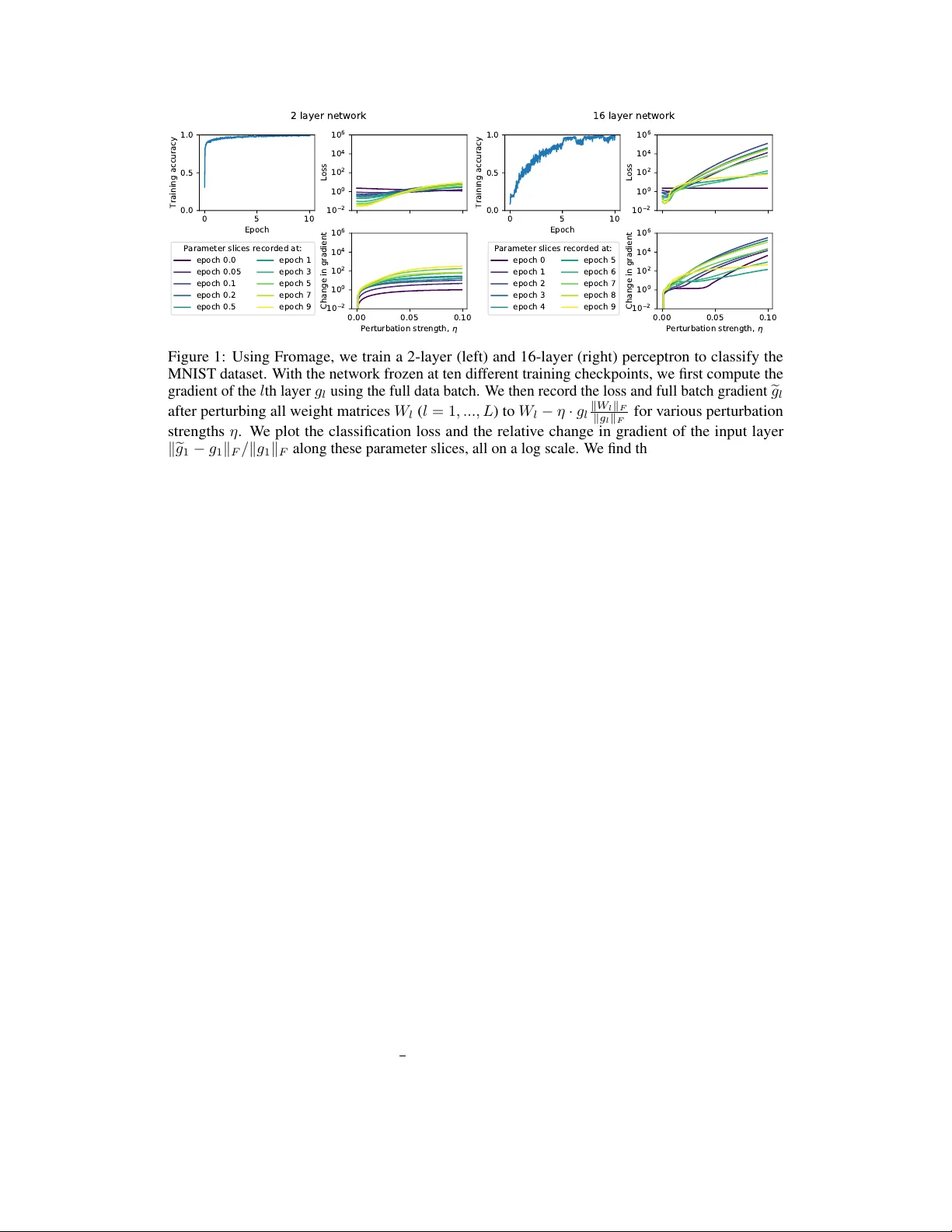
On the distance between two neural netw orks and the stability of lear ning Jer emy Bernstein Caltech bernstein@caltech.edu Arash V ahdat NVIDIA avahdat@nvidia.com Y isong Y ue Caltech yyue@caltech.edu Ming-Y u Liu NVIDIA mingyul@nvidia.com Abstract This paper relates parameter distance to gradient br eakdown for a broad class of nonlinear compositional functions. The analysis leads to a ne w distance function called deep r elative trust and a descent lemma for neural networks. Since the re- sulting learning rule seems to require little to no learning rate tuning, it may unlock a simpler workflo w for training deeper and more complex neural networks. The Python code used in this paper is here: https://github.com/jxbz/fromage . 1 Introduction Gradient descent is the workhorse of deep learning. T o decrease a loss function L ( W ) , this simple algorithm pushes the neural netw ork parameters W along the neg ativ e gradient of the loss. One motiv ation for this rule is that it minimises the local loss surf ace under a quadratic trust region [1]: W − η ∇L ( W ) | {z } gradient descent = W + arg min ∆ W h L ( W ) + ∇L ( W ) T ∆ W | {z } local loss surface + 1 2 η k ∆ W k 2 2 | {z } quadratic penalty i . (1) Since a quadratic trust region does not capture the compositional structure of a neural network, it is difficult to choose the learning rate η in practice. Goodfello w et al. [2, p. 424] advise: If you hav e time to tune only one hyperparameter , tune the learning rate. Practitioners usually resort to tuning η ov er a log arithmic grid. If that fails, they may try tuning a dif ferent optimisation algorithm such as Adam [ 3 ]. But the cost of grid search scales exponentially in the number of interacting neural networks, and state of the art techniques in v olving just two neural networks are dif ficult to tune [ 4 ] and often unstable [ 5 ]. Eliminating the need for learning rate grid search could enable new applications in volving multiple competiti ve and/or cooperativ e networks. W ith that goal in mind, this paper replaces the quadratic penalty appearing in Equation 1 with a novel distance function tailored to the compositional structure of deep neural networks. Our contributions: 1. By a direct perturbation analysis of the neural network function and Jacobian, we deri ve a distance on neural networks called deep r elative trust . 2. W e show how to combine deep relative trust with the fundamental theorem of calculus to deriv e a descent lemma tailored to neural networks. From the new descent lemma, we deriv e a learning algorithm that we call Frobenius matched gradient descent—or F r omage . Fromage’ s learning rate has a clear interpretation as controlling the relative size of updates. 3. While Fromage is similar to the LARS optimiser [ 6 ], we make the observ ation that Fromage works well across a range of standard neural network benchmarks—including generati ve adversarial networks and natural language transformers— without learning rate tuning . 34th Conference on Neural Information Processing Systems (NeurIPS 2020), V ancouver , Canada. 2 Entendámonos... ...so we understand each other . The goal of this section is to revie w a few basics of deep learning, including heuristics commonly used in algorithm design and areas where current optimisation theory falls short. W e shall see that a good notion of distance between neural networks is still a subject of acti ve research. Deep learning basics Deep learning seeks to fit a neur al network function f ( W ; x ) with parameters W to a dataset of N input-output pairs { x i , y i } N i =1 . If we let L i := L ( f i , y i ) measure the discrepancy between prediction f i := f ( W ; x i ) and target y i , then learning proceeds by gradient descent on the loss : P N i =1 L i . Though various neural network architectures exist, we shall focus our theoretical effort on the multilayer per ceptr on , which already contains the most striking features of general neural networks: matrices, nonlinearities, and layers. Definition 1 (Multilayer perceptron) . A multilayer perceptron is a function f : R n 0 → R n L composed of L layers. The l th layer is a linear map W l : R n l − 1 → R n l followed by a nonlinearity ϕ : R → R that is applied elementwise. W e may describe the network in two complementary ways: f ( x ) := ϕ ◦ W L | {z } layer L ◦ ϕ ◦ W L − 1 | {z } layer L − 1 ◦ ... ◦ ϕ ◦ W 1 | {z } layer 1 ( x ); ( L layer network) h l ( x ) := ϕ ( W l h l − 1 ( x )); h 0 ( x ) := x. (hidden layer recursion) Since we wish to fit the network via gradient descent, we shall be interested in the gradient of the loss with respect to the l th parameter matrix. This may be decomposed via the chain rule. Schematically: ∇ W l L = ∂ L ∂ f · ∂ f ∂ h l · ϕ 0 ( W l h l − 1 ) · h l − 1 . (2) The famous backpropagation algorithm [ 7 ] observes that the second term may be decomposed o ver the layers of the network. Following the notation of Pennington et al. [8]: Proposition 1 (Jacobian of the multilayer perceptron) . Consider a multilayer perceptr on with L layers. The layer- l -to-output Jacobian J l is given by: J l := ∂ f ( x ) ∂ h l = ∂ f ∂ h L − 1 · ∂ h L − 1 ∂ h L − 2 · ... · ∂ h l +1 ∂ h l = Φ 0 L W L · Φ 0 L − 1 W L − 1 · ... · Φ 0 l +1 W l +1 , wher e Φ 0 k := diag h ϕ 0  W k h k − 1 ( x )  i denotes the derivative of the nonlinearity at the k th layer . A key observ ation is that the network function f and Jacobian ∂ f ∂ h l share a common mathematical structure—a deep, layered composition. W e shall exploit this in our theory . Empirical deep learning The formulation of gradient descent giv en in Equation 1 quickly encounters a problem known as the vanishing and exploding gradient pr oblem , where the scale of updates becomes miscalibrated with the scale of parameters in different layers of the network. Common tricks to ameliorate the problem include careful choice of weight initialisation [ 9 ], di viding out the gradient scale [ 3 ], gradient clipping [ 10 ] and directly controlling the relativ e size of updates to each layer [ 6 , 11 ]. Each of these techniques has been adopted in numerous deep learning applications. Still, there is a cost to using heuristic techniques. For instance, techniques that rely on careful initialisation may break down by the end of training, leading to instabilities that are difficult to trace. These heuristics also lead to a proliferation of hyperparameters that are difficult to interpret and tune. W e may wonder , why does our optimisation theory not handle these matters for us? 2 Deep learning optimisation theory It is common in optimisation theory to assume that the loss has Lipschitz continuous gradients: k∇L ( W + ∆ W ) − ∇L ( W ) k 2 ≤ 1 η k ∆ W k 2 . By a standard ar gument in volving the quadratic penalty mentioned in the introduction, this assumption leads to gradient descent [ 1 ]. This assumption is ubiquitous to the point that it is often just referred to as smoothness [ 12 ]. It is used in a number of w orks in the context of deep learning optimisation [12 – 15], distributed training [16], and generati ve adversarial networks [17]. W e conduct an empirical study that shows that neural networks do not hav e Lipschitz continuous gradients in practice. W e do this for a 16 layer multilayer perceptron (Figure 1), and find that the gradient grows roughly exponentially in the size of a perturbation. See [ 18 ] for more empirical in vestigation, and [19] for more discussion on this point. Sev eral classical optimisation frameworks go beyond the quadratic penalty k ∆ W k 2 2 of Equation 1: 1. Mirror descent [ 20 ] replaces k ∆ W k 2 2 by a Br e gman diver gence appropriate to the geometry of the problem. This framework w as studied in relation to deep learning [ 21 , 22 ], but it is still unclear whether there is a Bregman di ver gence that models the compositional structure of neural networks. 2. Natural gradient descent [ 23 ] replaces k ∆ W k 2 2 by ∆ W T F ∆ W . The Riemannian metric F ∈ R d × d should capture the geometry of the d -dimensional function class. Unfortunately , ev en writing down a d × d matrix is intractable for modern neural netw orks. Whilst some works explore tractable approximations [ 24 ], natural gradient descent is still a quadratic model of trust—we find that trust is lost far more catastrophically in deep networks. 3. Steepest descent [ 25 ] replaces k ∆ W k 2 2 by an arbitrary distance function. Neyshabur et al. [26] explore this approach using a rescaling in variant norm on paths through the network. The downside to the freedom of steepest descent is that it does not operate from first principles—so the chosen distance function may not match up to the problem at hand. Other work operates outside of these frameworks. Sev eral papers study the effect of architectural decisions on signal propagation through the network [ 8 , 27 – 30 ], though these works usually neglect functional distance and curv ature of the loss surface. Pennington and Bahri [31] do study curv ature, but rely on random matrix models to mak e progress. Generative adv ersarial networks Neural networks can learn to generate samples from comple x distributions. Generativ e adversarial learning [ 32 ] trains a discriminator netw ork D to classify data as real or fak e, and a generator network G is trained to fool D . Competition driv es learning in both netw orks. Letting V denote the success rate of the discriminator , the learning process is described as: min G max D V ( G, D ) . Defining the optimal discriminator for a given generator as D ∗ ( G ) := arg max D V ( G, D ) . Then generativ e adversarial learning reduces to a straightforward minimisation o ver the parameters of the generator: min G max D V ( G, D ) ≡ min G V ( G, D ∗ ( G )) . In practice this is solv ed as an inner -loop, outer -loop optimisation procedure where k steps of gradient descent are performed on the discriminator , follo wed by 1 step on the generator . For e xample, Miyato et al. [33] take k = 5 and Brock et al. [5] take k = 2 . For small k , this procedure is only well founded if the perturbation ∆ G to the generator is small so as to induce a small perturbation in the optimal discriminator . In symbols, we hope that: k ∆ G k  1 = ⇒ k D ∗ ( G + ∆ G ) − D ∗ ( G ) k  1 . But what does k ∆ G k mean? In what sense should it be small? W e see that this is another area that could benefit from an appropriate notion of distance on neural networks. 3 3 The distance between networks Suppose that a teacher wishes to assess a student’s learning. T raditionally , they will assign the student homework and trac k their pr ogr ess. What if, instead, they could peer inside the student’ s head and observe change dir ectly in the synapses—would that not be better for everyone? W e would like to establish a meaningful notion of functional distance for neural networks. This should let us know how far we can safely perturb a network’ s weights without needing to tune a learning rate and measure the effect on the loss empirically . The quadratic penalty of Equation 1 is akin to assuming a Euclidean structure on the parameter space, where the squared Euclidean length of a parameter perturbation determines how fast the loss function breaks do wn. The main pitfall of this assumption is that it does not reflect the deep compositional structure of a neural network. W e propose a new trust concept called deep relative trust . In this section, we shall motiv ate deep relative trust—the formal definition shall come in Section 4. Deep relativ e trust will in volv e a product over relati ve perturbations to each layer of the network. For a first glimpse of how this structure arises, consider a simple network that multiplies its input x ∈ R by two scalars a, b ∈ R . That is f ( x ) = a · b · x . Also consider perturbed function e f ( x ) = e a · e b · x where e a := a + ∆ a and e b := b + ∆ b . Then the relativ e dif ference obeys: | e f ( x ) − f ( x ) | | f ( x ) | ≤  1 + | ∆ a | | a |   1 + | ∆ b | | b |  − 1 . (3) The simple deri vation may be found at the be ginning of Appendix B. The ke y point is that the relati ve change in the composition of two operators depends on the product of the relative change in each operator . The same structure extends to the relati ve distance between two neural netw orks—both in terms of function and gradient—as we will now demonstrate. Theorem 1. Let f be a multilayer per ceptron with nonlinearity ϕ and L weight matrices { W l } L l =1 . Let e f be a second network with the same ar chitectur e but differ ent weight matrices { f W l } L l =1 . F or con venience, define layerwise perturbation matrices { ∆ W l := f W l − W l } L l =1 . Further suppose that the following two conditions hold: 1. T ransmission. There e xist α, β ≥ 0 such that ∀ x, y : α · k x k 2 ≤ k ϕ ( x ) k 2 ≤ β · k x k 2 ; α · k x − y k 2 ≤ k ϕ ( x ) − ϕ ( y ) k 2 ≤ β · k x − y k 2 . 2. Conditioning. All matrices { W l } L l =1 , { f W l } L l =1 and perturbations { ∆ W l } L l =1 have condition number (ratio of lar gest to smallest singular value) no lar ger than κ . Then a) for all non-zer o inputs x ∈ R n 0 , the r elative functional differ ence obeys: k e f ( x ) − f ( x ) k 2 k f ( x ) k 2 ≤  β α κ 2  L " L Y k =1  1 + k ∆ W k k F k W k k F  − 1 # . And b) the layer- l -to-output J acobian satisfies:    ∂ e f ∂ e h l − ∂ f ∂ h l    F    ∂ f ∂ h l    F ≤  β α κ 2  L − l " L Y k = l +1 β α  1 + k ∆ W k k F k W k k F  − 1 # . The proof is giv en in the appendix. The closest existing result that we are aware of is [ 34 , Lemma 2], which bounds functional distance b ut not Jacobian distance. Also, since [ 34 , Lemma 2] only holds for small perturbations, it misses the product structure of Theorem 1. It is the product structure that encodes the interactions between perturbations to different layers. In words, Theorem 1 says that the relati ve change of a multilayer perceptron in terms of both function and gradient is controlled by a product ov er relati ve perturbations to each layer . Bounding the relati ve 4 0 5 10 Epoch 0.0 0.5 1.0 Training accuracy 1 0 2 1 0 0 1 0 2 1 0 4 1 0 6 Loss 0.00 0.05 0.10 P e r t u r b a t i o n s t r e n g t h , 1 0 2 1 0 0 1 0 2 1 0 4 1 0 6 Change in gradient Parameter slices recorded at: epoch 0.0 epoch 0.05 epoch 0.1 epoch 0.2 epoch 0.5 epoch 1 epoch 3 epoch 5 epoch 7 epoch 9 2 layer network 0 5 10 Epoch 0.0 0.5 1.0 Training accuracy 1 0 2 1 0 0 1 0 2 1 0 4 1 0 6 Loss 0.00 0.05 0.10 P e r t u r b a t i o n s t r e n g t h , 1 0 2 1 0 0 1 0 2 1 0 4 1 0 6 Change in gradient Parameter slices recorded at: epoch 0 epoch 1 epoch 2 epoch 3 epoch 4 epoch 5 epoch 6 epoch 7 epoch 8 epoch 9 16 layer network Figure 1: Using Fromage, we train a 2-layer (left) and 16-layer (right) perceptron to classify the MNIST dataset. W ith the network frozen at ten dif ferent training checkpoints, we first compute the gradient of the l th layer g l using the full data batch. W e then record the loss and full batch gradient e g l after perturbing all weight matrices W l ( l = 1 , ..., L ) to W l − η · g l k W l k F k g l k F for v arious perturbation strengths η . W e plot the classification loss and the relativ e change in gradient of the input layer k e g 1 − g 1 k F / k g 1 k F along these parameter slices, all on a log scale. W e find that the loss and relativ e change in gradient grow quasi-e xponentially when the perceptron is deep, suggesting that Euclidean trust is violated. As such, these results are more consistent with our notion of deep relativ e trust. change in function f in terms of the relativ e change in parameters W is reminiscent of a concept from numerical analysis known as the r elative condition number . The relativ e condition number of a numerical technique measures the sensiti vity of the technique to input perturbations. This suggests that we may think of Theorem 1 as establishing the relati ve condition number of a neural network with respect to parameter perturbations. The two most striking consequences of Theorem 1 are that for a multilayer perceptron: 1. The trust region is not quadratic, but rather quasi-exponential at lar ge depth L . 2. The trust region depends on the relativ e strength of perturbations to each layer . T o validate these theoretical consequences, Figure 1 displays the results of an empirical study . For two multilayer perceptrons of depth 2 and 16, we measured the stability of the loss and gradient to perturbation at various stages of training. For the depth 16 network, we found that the loss and gradient did break do wn quasi-exponentially in the layerwise relativ e size of a parameter perturbation. For the depth 2 network, the breakdo wn was much milder . W e will now discuss the plausibility of the assumptions made in Theorem 1. The first assumption amounts to assuming that the nonlinearity must transmit a certain fraction of its input. This is satisfied, for example, by the “leak y relu” nonlinearity , where for 0 < a ≤ 1 : leaky _ relu( x ) :=  x if x ≥ 0; ax if x < 0 . Many nonlinearities only transmit half of their input domain—for e xample, the relu nonlinearity: relu( x ) := max(0 , x ) . Although relu is technically not cov ered by Theorem 1, we may model the fact that it transmits half its input domain by setting α = β = 1 2 . The second assumption is that all weight matrices and perturbations are full rank. In general this assumption may be violated. But provided that a small amount of noise is present in the updates, then by smoothed analysis of the matrix condition number [35, 36] it may often hold in practice. 5 4 Descent under deep relati ve trust In the last section we studied the relativ e functional dif ference and gradient difference between tw o neural networks. Whilst the relativ e breakdown in gradient is intuitiv ely an important object for optimisation theory , to make this intuition rigorous we ha ve deri ved the follo wing lemma: Lemma 1. Consider a continuously differ entiable function L : R n → R that maps W 7→ L ( W ) . Suppose that parameter vector W decomposes into L parameter gr oups: W = ( W 1 , W 2 , ..., W L ) , and consider making a perturbation ∆ W = (∆ W 1 , ∆ W 2 , ..., ∆ W L ) . Let θ l measur e the angle between ∆ W l and ne gative gradient − g l ( W ) := −∇ W l L ( W ) . Then: L ( W + ∆ W ) − L ( W ) ≤ − L X l =1 k g l ( W ) k F k ∆ W l k F  cos θ l − max t ∈ [0 , 1] k g l ( W + t ∆ W ) − g l ( W ) k F k g l ( W ) k F  . In words, the inequality says that the change in a function due to an input perturbation is bounded by the product of three terms, summed o ver parameter groups. The first two terms measure the size of the gradient and the size of the perturbation. The third term is a tradeoff between ho w aligned the perturbation is with the gradient, and ho w fast the gradient breaks do wn. Informally , the result says: to r educe a function, follow the ne gative gradient until it br eaks down . Descent is guaranteed when the bracketed term in Lemma 1 is positi ve. That is, for l = 1 , ..., L : max t ∈ [0 , 1] k g l ( W + t ∆ W ) − g l ( W ) k F k g l ( W ) k F < cos θ l . (4) Geometrically this condition requires that, for ev ery parameter group, the maximum change in gradient along the perturbation be smaller than the projection of the gradient in that direction. The simplest strategy to meet this condition is to choose ∆ W l = − η g l ( W ) . The learning rate η must be chosen small enough such that, for all parameter groups l , the lefthand side of (4) is smaller than cos θ l = 1 . This is what is done in practice when gradient descent is used to train neural networks. T o do better than blindly tuning the learning rate in gradient descent, we need a way to estimate the relative gradient breakdown that appears in (4). The gradient of the loss is decomposed in Equation 2—let us inspect that result. Three of the four terms in volve either a network Jacobian or a subnetwork output, for which relati ve change is governed by Theorem 1. Since Theorem 1 gov erns relativ e change in three of the four terms in Equation 2, we propose extending it to cov er the whole expression—we call this modelling assumption deep r elative trust . Modelling assumption 1 (Deep relativ e trust) . Consider a neural network with L layers and param- eters W = ( W 1 , W 2 , ..., W L ) . Consider parameter perturbation ∆ W = (∆ W 1 , ∆ W 2 , ..., ∆ W L ) . Let g l denote the gradient of the network loss function L with r espect to parameter matrix W l . Then the gradient br eakdown is bounded by: k g l ( W + ∆ W ) − g l ( W ) k F k g l ( W ) k F ≤ L Y k =1  1 + k ∆ W k k F k W k k F  − 1 . Deep relati ve trust applies the functional form that appears in Theorem 1 to the gradient of the loss function. As compared to Theorem 1, we have set α = β = 1 2 (a model of relu) and κ = 1 (a model of well-conditioned matrices). Another reason that deep relati ve trust is a model rather than a theor em is that we ha ve neglected the ∂ L /∂ f term in Equation 2 which depends on the choice of loss function. Giv en that deep relativ e trust appears to penalise the relativ e size of perturbations to each layer , it is natural that our learning algorithm should account for this by ensuring that layerwise perturbations are bounded like k ∆ W l k F / k W l k F ≤ η for some small η > 0 . The following lemma formalises this idea. As far as we are aw are, this is the first descent lemma tailored to the neural network structure. Lemma 2. Let L be a continuously differ entiable loss function for a neural network of depth L that obe ys deep r elative trust. Consider a perturbation ∆ W = (∆ W 1 , ∆ W 2 , ..., ∆ W L ) to the parameter s W = ( W 1 , W 2 , ..., W L ) with layerwise bounded r elative size, meaning that k ∆ W l k F / k W l k F ≤ η for l = 1 , ..., L . Let θ l measur e the angle between ∆ W l and − g l ( W ) . The perturbation will decr ease the loss function pr ovided that for all l = 1 , ..., L : η < (1 + cos θ l ) 1 L − 1 . 6 Algorithm 1 F r omage —a good def ault η = 0 . 01 . Input: learning rate η and matrices { W l } L l =1 repeat collect gradients { g l } L l =1 for layer l = 1 to L do W l ← 1 √ 1+ η 2 h W l − η · k W l k F k g l k F · g l i end for until con verged 0 50 100 Epoch 0.0 0.1 0.2 0.3 0.4 Layerwise parameter norms Fromage 0 50 100 Epoch LARS Figure 2: Left: the Fromage optimiser . Fromage differs to LARS [ 6 ] by the 1 / p 1 + η 2 prefactor . Right: without the prefactor , LARS suffers compounding gro wth in rescaling in v ariant layers that ev entually leads to numerical overflo w . This example is for a spectrally normalised cGAN [33, 37]. 5 Frobenius matched gradient descent In the pre vious section we established a descent lemma that tak es into account the neural network structure. It is now time to apply that lemma to deri ve a learning algorithm. The principle that we shall adopt is to make the lar gest perturbation that still guarantees descent by Lemma 2. T o do this, we need to set cos θ l = 1 whilst maintaining k ∆ W l k F ≤ η k W l k F for e very layer l = 1 , ..., L . This is achiev ed by the follo wing update: ∆ W l = − η · k W l k F k g l k F · g l for l = 1 , ..., L. (5) This learning rule is similar to LARS (layerwise adapti ve rate scaling) proposed on empirical grounds by Y ou et al. [6]. The authors demonstrated that LARS stabilises large batch network training. Unfortunately , there is still an issue with this update rule that needs to be addressed. Neural network layers that in volve batc h norm [ 38 ] or spectral norm [ 33 ] are in v ariant to the rescaling map W l → W l + α W l and therefore the corresponding gradient g l must lie orthogonal to W l . This means that the learning rule in Equation 2 will increase weight norms in these layers by a constant factor ev ery iteration. T o see this, we argue by Pythagoras’ theorem combined with Equation 5: k W l + ∆ W l k 2 F = k W l k 2 F + k ∆ W l k 2 F = (1 + η 2 ) k W l k 2 F . k ∆ W l k F k W l k F p 1 + η 2 · k W l k F This is compounding gr owth meaning that it will lead to numerical ov erflow if left unchecked. W e empirically validate this phenomenon in Figure 2. One way to solve this problem is to introduce and tune an additional weight decay hyperparameter , and this is the strate gy adopted by LARS. In this work we are seeking to dispense with unnecessary hyperparameters, and therefore we propose explicitly correcting this instability via an appropriate prefactor . W e call our algorithm Frobenius matched gradient descent—or F r omage . See Algorithm 1 above. The attractiv e feature of Algorithm 1 is that there is only one hyperparameter and its meaning is clear . Neglecting the second order correction, we hav e that for every layer l = 1 , ..., L , the algorithm’ s update satisfies: k ∆ W l k F k W l k F = η . (6) In w ords: the algorithm induces a relati ve change of η in each layer of the neural network per iteration. 7 0 10 20 30 40 50 N u m b e r o f l a y e r s , L 0.2 0.4 0.6 0.8 1.0 Training accuracy SGD Fromage Adam 0 10 20 30 40 50 N u m b e r o f l a y e r s , L 0.2 0.4 0.6 0.8 1.0 Training accuracy Fromage learning rate = 0 . 1 = 0 . 0 1 = 0 . 0 0 1 Figure 3: T raining multilayer perceptrons at depths challenging for existing optimisers. W e train multilayer perceptrons of depth L on the MNIST dataset. At each depth, we plot the training accuracy after 100 epochs. Left: for each algorithm, we plot the best performing run over 3 learning rate settings found to be appropriate for that algorithm. W e also plot trend lines to help guide the eye. Right: the Fromage results are presented for each learning rate setting. Since for deeper networks a smaller value of η was needed in Fromage, these results provide partial support for Lemma 2. 1 0 4 1 0 3 1 0 2 1 0 1 1 0 0 L e a r n i n g r a t e 0.0 0.5 1.0 B e s t e r r o r / e r r o r SGD 1 0 4 1 0 3 1 0 2 1 0 1 1 0 0 L e a r n i n g r a t e Fromage CIFAR-10 GAN Transformer 1 0 4 1 0 3 1 0 2 1 0 1 1 0 0 L e a r n i n g r a t e Adam Figure 4: Learning rate tuning for standard benchmarks. For each learning rate setting η , we plot the error at the best tuned η divided by the error for that η , so that a value of 1.0 corresponds to the best learning rate setting for that task. For Fromage, the setting of η = 0 . 01 was optimal across all tasks. 6 Empirical study T o test the main prediction of our theory—that the function and gradient of a deep network break down quasi-exponentially in the size of the perturbation—we directly study the behaviour of a multilayer perceptron trained on the MNIST dataset [ 39 ] under parameter perturbations. Perturbing along the gradient direction, we find that for a deep network the change in gradient and objective function indeed grow quasi-e xponentially in the relative size of a parameter perturbation (Figure 1). The theory also predicts that the geometry of trust becomes increasingly pathological as the network gets deeper , and Fromage is specifically designed to account for this. As such, it should be easier to train very deep networks with Fromage than by using other optimisers. T esting this, we find that off-the-shelf optimisers are unable to train multilayer perceptrons (without batch norm [ 38 ] or skip connections [40]) ov er 25 layers deep; Fromage was able to train up to at least depth 50 (Figure 3). Next, we benchmark Fromage on four canonical deep learning tasks: classification of CIF AR-10 & ImageNet, generativ e adversarial network (GAN) training on CIF AR-10, and transformer training on W ikitext-2. In theory , Fromage should be easy to use because its one hyperparameter is meaningful for neural networks and is governed by a descent lemma (Lemma 2). The results are giv en in T able 1. Since this paper is about optimisation, all results are reported on the training set. T est set results and full experimental details are gi ven in Appendix C. Fromage achie ved lo wer training error than SGD on all four tasks (and by a substantial margin on three tasks). Fromage also outperformed Adam on three out of four tasks. Most importantly , Fromage used the same learning rate η = 0 . 01 across all tasks. In contrast, the learning rate in SGD and Adam needed to be carefully tuned, as sho wn in Figure 4. Note that for all algorithms, η was decayed by 10 when the loss plateaued. It should be noted that in preliminary runs of both the CIF AR-10 and Transformer experiments, Fromage would heavily overfit the training set. W e were able to correct this behaviour for the results presented in T ables 1 and 2 by constraining the neural architecture. In particular , each layer’ s parameter norm was constrained to be no lar ger than its norm at initialisation. 8 T able 1: Training results. W e quote loss for the classifiers, FID [ 4 ] for the GAN, and perplexity for the transformer—so lo wer is better . T est results and experimental details are gi ven in Appendix C. For all algorithms, η was decayed by 10 when the loss plateaued. Benchmark SGD η Fromage η Adam η SGD Fromage Adam CIF AR-10 0.1 0.01 0.001 (1 . 5 ± 0 . 2) × 10 − 4 (2 . 5 ± 0 . 5) × 10 − 5 (2 . 5 ± 0 . 5) × 10 − 5 (2 . 5 ± 0 . 5) × 10 − 5 (6 ± 3) × 10 − 5 ImageNet 1.0 0.01 0.001 2 . 020 ± 0 . 003 2 . 001 ± 0 . 001 2 . 001 ± 0 . 001 2 . 001 ± 0 . 001 2 . 02 ± 0 . 01 GAN 0.01 0.01 0.0001 34 ± 2 16 ± 1 16 ± 1 16 ± 1 23 . 7 ± 0 . 7 T ransformer 1.0 0.01 0.001 150 . 0 ± 0 . 3 66 . 1 ± 0 . 1 36 . 8 ± 0 . 1 36 . 8 ± 0 . 1 36 . 8 ± 0 . 1 7 Discussion The effort to alleviate learning rate tuning in deep learning is not new . For instance, Schaul et al. [41] tackled this problem in a paper titled “No More Pesky Learning Rates”. Nonetheless—in practice—the need for learning rate tuning has persisted [ 2 ]. Then what sets our paper apart? The main contrib ution of our paper is its ef fort to explicitly model deep netw ork gradients via deep relative trust , and to connect this model to the simple Fromage learning rule. In contrast, Schaul et al.’ s work relies on estimating curv ature information in an online fashion—thus incurring computational ov erhead while not providing clear insight on the meaning of the learning rate for neural networks. T o what extent may our paper eliminate pesky learning rates? Lemma 2 and the experiments in Figure 3 suggest that—for multilayer perceptrons—Fromage’ s optimal learning rate should depend on network depth. Ho wev er , the results in T able 1 show that across a variety of more practically interesting benchmarks, Fromage’ s initial learning rate did not require tuning. It is important to point out that these practical benchmarks employ more in volved network architectures than a simple multilayer perceptron. For instance, the y use skip connections [ 40 ] which allo w signals to skip layers. Future work could in vestigate how skip connections af fect the deep relati ve trust model: an intuitiv e hypothesis is that they reduce some notion of ef fective depth of very deep netw orks. In conclusion, we ha ve deri ved a distance on deep neural networks called deep r elative trust . W e used this distance to deri ve a descent lemma for neural netw orks and a learning rule called F roma ge . While the theory suggests a depth-dependent learning rate for multilayer perceptrons, we found that Fromage did not require learning rate tuning in our experiments on more modern network architectures. Broader impact This paper aims to improve our foundational understanding of learning in neural networks. This could lead to many unforeseen consequences down the line. An immediate practical outcome of the work is a learning rule that seems to require less hyperparameter tuning than stochastic gradient descent. This may hav e the following consequences: • Network training may become less time and energy intensi ve. • It may become easier to train and deploy neural networks without human oversight. • It may become possible to train more complex network architectures to solve ne w problems. In short, this paper could make a po werful tool both easier to use and easier to abuse. Acknowledgements and disclosur e of funding The authors would like to thank Rumen Dango vski, Dillon Huf f, Jeffre y Pennington, Florian Schaefer and Joel T ropp for useful con versations. They made heavy use of a codebase b uilt by Jiahui Y u. They are grateful to Si vakumar Arayandi Thottakara, Jan Kautz, Sabu Nadarajan and Nithya Natesan for infrastructure support. JB was supported by an NVIDIA fello wship, and this work was funded in part by N ASA. 9 References [1] Léon Bottou, Frank E. Curtis, and Jor ge Nocedal. Optimization methods for large-scale machine learning. SIAM Revie w , 2016. [2] Ian Goodfellow , Y oshua Bengio, and Aaron Courville. Deep Learning . MIT Press, 2016. http://www.deeplearningbook.org . [3] Diederik P . Kingma and Jimmy Ba. Adam: A Method for Stochastic Optimization. In International Confer ence on Learning Repr esentations , 2015. [4] Martin Heusel, Hubert Ramsauer , Thomas Unterthiner , Bernhard Nessler , and Sepp Hochreiter . GANs trained by a two time-scale update rule con ver ge to a local Nash equilibrium. In Neural Information Pr ocessing Systems , 2017. [5] Andrew Brock, Jef f Donahue, and Karen Simonyan. Large scale GAN training for high fidelity natural image synthesis. In International Confer ence on Learning Repr esentations , 2019. [6] Y ang Y ou, Igor Gitman, and Boris Ginsburg. Scaling SGD batch size to 32K for Imagenet training. T echnical Report UCB/EECS-2017-156, University of California, Berk eley , 2017. [7] David E. Rumelhart, Geof frey E. Hinton, and Ronald J. W illiams. Learning representations by back-propagating errors. Nature , 1986. [8] Jeffre y Pennington, Samuel Schoenholz, and Surya Ganguli. Resurrecting the sigmoid in deep learning through dynamical isometry: theory and practice. In Neural Information Pr ocessing Systems , 2017. [9] Xavier Glorot and Y oshua Bengio. Understanding the difficulty of training deep feedforward neural networks. In International Conference on Artificial Intellig ence and Statistics , 2010. [10] Razvan Pascanu, T omas Mikolo v , and Y oshua Bengio. On the difficulty of training recurrent neural networks. In International Conference on Mac hine Learning , 2013. [11] Y ang Y ou, Jing Li, Sashank Reddi, Jonathan Hseu, Sanji v Kumar , Srinadh Bhojanapalli, Xiaodan Song, James Demmel, Kurt Keutzer , and Cho-Jui Hsieh. Lar ge batch optimization for deep learning: Training BER T in 76 minutes. In International Confer ence on Learning Repr esentations , 2020. [12] Moritz Hardt, Ben Recht, and Y oram Singer . Train faster , generalize better: Stability of stochastic gradient descent. In International Confer ence on Machine Learning , 2016. [13] Zeyuan Allen-Zhu. Natasha 2: Faster non-con vex optimization than SGD. In Neural Information Pr ocessing Systems , 2018. [14] Simon S. Du, Chi Jin, Jason D. Lee, Michael I. Jordan, Aarti Singh, and Barnabas Poczos. Gradient descent can take exponential time to escape saddle points. In Neural Information Pr ocessing Systems , 2017. [15] Jason D. Lee, Max Simchowitz, Michael I. Jordan, and Benjamin Recht. Gradient descent only con verges to minimizers. In Conference on Learning Theory , 2016. [16] Jeremy Bernstein, Y u-Xiang W ang, Kamyar Azizzadenesheli, and Animashree Anandkumar . signSGD: Compressed optimisation for non-con ve x problems. In International Confer ence on Machine Learning , 2018. [17] Florian Schaefer and Anima Anandkumar . Competitive gradient descent. In Neural Information Pr ocessing Systems , 2019. [18] Ari Benjamin, Da vid Rolnick, and K onrad K ording. Measuring and regularizing networks in function space. In International Confer ence on Learning Repr esentations , 2019. [19] Ruoyu Sun. Optimization for deep learning: theory and algorithms. , 2019. 10 [20] Arkady S. Nemirovsky and David B. Y udin. Problem complexity and method efficiency in optimization . W iley , 1983. [21] Navid Azizan and Babak Hassibi. Stochastic gradient/mirror descent: Minimax optimality and implicit regularization. In International Conference on Learning Repr esentations , 2019. [22] Navid Azizan, Sahin Lale, and Babak Hassibi. Stochastic mirror descent on overparameterized nonlinear models: Conv ergence, implicit re gularization, and generalization. , 2019. [23] Shunichi Amari. Information geometry and its applications . Springer , 2016. [24] James Martens and Roger Grosse. Optimizing neural networks with Kronecker-factored approximate curvature. In International Confer ence on Machine Learning , 2015. [25] Stephen Boyd and Lie ven V andenberghe. Conve x Optimization . Cambridge University Press, 2004. [26] Behnam Neyshab ur, Ruslan Salakhutdinov , and Nathan Srebro. Path-SGD: Path-normalized optimization in deep neural networks. In Neural Information Pr ocessing Systems , 2015. [27] Cem Anil, James Lucas, and Roger Grosse. Sorting out Lipschitz function approximation. In International Confer ence on Machine Learning , 2019. [28] Andrew M. Saxe, James L. McClelland, and Surya Ganguli. Exact solutions to the nonlinear dynamics of learning in deep linear neural networks. In International Confer ence on Learning Repr esentations , 2014. [29] Lechao Xiao, Y asaman Bahri, Jascha Sohl-Dickstein, Samuel Schoenholz, and Jeffrey Penning- ton. Dynamical isometry and a mean field theory of CNNs: How to train 10,000-layer v anilla con volutional neural networks. In International Conference on Mac hine Learning , 2018. [30] Ge Y ang and Samuel Schoenholz. Mean field residual networks: On the edge of chaos. In Neural Information Pr ocessing Systems , 2017. [31] Jeffre y Pennington and Y asaman Bahri. Geometry of neural network loss surfaces via random matrix theory . In International Confer ence on Machine Learning , 2017. [32] Ian Goodfellow , Jean Pouget-Abadie, Mehdi Mirza, Bing Xu, David W arde-Farley , Sherjil Ozair , Aaron Courville, and Y oshua Bengio. Generativ e adversarial nets. In Neural Information Pr ocessing Systems , 2014. [33] T akeru Miyato, T oshiki Kataoka, Masanori Koyama, and Y uichi Y oshida. Spectral normalization for generativ e adversarial networks. In International Confer ence on Learning Repr esentations , 2018. [34] Behnam Neyshab ur, Srinadh Bhojanapalli, and Nathan Srebro. A P A C-bayesian approach to spectrally-normalized margin bounds for neural networks. In International Conference on Learning Repr esentations , 2018. [35] Peter Bürgisser and Felipe Cucker . Smoothed analysis of Moore-Penrose in version. SIAM Journal on Matrix Analysis and Applications , 2010. [36] Arvind Sankar , Daniel A. Spielman, and Shang-Hua T eng. Smoothed analysis of the condition numbers and gro wth factors of matrices. SIAM Journal on Matrix Analysis and Applications , 2006. [37] T akeru Miyato and Masanori K oyama. cGANs with projection discriminator . In International Confer ence on Learning Repr esentations , 2018. [38] Serge y Ioffe and Christian Sze gedy . Batch normalization: Accelerating deep network training by reducing internal cov ariate shift. In International Conference on Mac hine Learning , 2015. [39] Y ann LeCun, Leon Bottou, Y oshua Bengio, and Patrick Haffner. Gradient-based learning applied to document recognition. Pr oceedings of the IEEE , 1998. 11 [40] Kaiming He, Xiangyu Zhang, Shaoqing Ren, and Jian Sun. Deep residual learning for image recognition. In Computer V ision and P attern Recognition , 2016. [41] T om Schaul, Sixin Zhang, and Y ann LeCun. No more pesky learning rates. In International Confer ence on Machine Learning , 2013. [42] Alex Krizhevsky . Learning multiple layers of features from tiny images. T echnical report, Univ ersity of T oronto, 2009. [43] Christian Sze gedy , V incent V anhoucke, Ser gey Iof fe, Jon Shlens, and Zbignie w W ojna. Rethink- ing the Inception architecture for computer vision. In Computer V ision and P attern Recognition , 2015. [44] T ero Karras, T imo Aila, Samuli Laine, and Jaakko Lehtinen. Progressiv e growing of GANs for improv ed quality , stability , and variation. In International Conference on Learning Repr esenta- tions , 2018. [45] Olga Russako vsky , Jia Deng, Hao Su, Jonathan Krause, Sanjeev Satheesh, Sean Ma, Zhiheng Huang, Andrej Karpathy , Aditya Khosla, Michael Bernstein, Alexander C. Berg, and Li Fei-Fei. ImageNet large scale visual recognition challenge. International Journal of Computer V ision , 2015. [46] Ashish V aswani, Noam Shazeer , Niki Parmar , Jakob Uszkoreit, Llion Jones, Aidan N Gomez, Łukasz Kaiser , and Illia Polosukhin. Attention is all you need. In Neural Information Pr ocessing Systems , 2017. [47] Stephen Merity , Caiming Xiong, James Bradbury , and Richard Socher . Pointer sentinel mixture models. In International Confer ence on Learning Repr esentations , 2017. 12 A ppendix A A descent lemma f or neural networks Lemma 1. Consider a continuously differ entiable function L : R n → R that maps W 7→ L ( W ) . Suppose that parameter vector W decomposes into L parameter gr oups: W = ( W 1 , W 2 , ..., W L ) , and consider making a perturbation ∆ W = (∆ W 1 , ∆ W 2 , ..., ∆ W L ) . Let θ l measur e the angle between ∆ W l and ne gative gradient − g l ( W ) := −∇ W l L ( W ) . Then: L ( W + ∆ W ) − L ( W ) ≤ − L X l =1 k g l ( W ) k F k ∆ W l k F  cos θ l − max t ∈ [0 , 1] k g l ( W + t ∆ W ) − g l ( W ) k F k g l ( W ) k F  . Pr oof. By the fundamental theorem of calculus, L ( W + ∆ W ) − L ( W ) = L X l =1 g l ( W ) T ∆ W l + Z 1 0  g l ( W + t ∆ W ) − g l ( W )  T ∆ W l d t. The result follows by replacing the first term on the righthand side by the cosine formula for the dot product, and bounding the second term via the integral estimation lemma. Lemma 2. Let L be a continuously differ entiable loss function for a neural network of depth L that obe ys deep r elative trust. Consider a perturbation ∆ W = (∆ W 1 , ∆ W 2 , ..., ∆ W L ) to the parameter s W = ( W 1 , W 2 , ..., W L ) with layerwise bounded r elative size, meaning that k ∆ W l k F / k W l k F ≤ η for l = 1 , ..., L . Let θ l measur e the angle between ∆ W l and − g l ( W ) . The perturbation will decr ease the loss function pr ovided that for all l = 1 , ..., L : η < (1 + cos θ l ) 1 L − 1 . Pr oof. Using the gradient reliability estimate from deep relativ e trust, we obtain that: max t ∈ [0 , 1] k g l ( W + t ∆ W ) − g l ( W ) k 2 k g l ( W ) k 2 ≤ max t ∈ [0 , 1] L Y k =1  1 + k t ∆ W k k F k W k k F  − 1 ≤ L Y k =1  1 + k ∆ W k k F k W k k F  − 1 . T o guarantee descent, we require that the bracketed term in Lemma 1 is positi ve for all l = 1 , ..., L . By the previous inequality , this will occur provided that for all l = 1 , ..., L : L Y k =1  1 + k ∆ W k k F k W k k F  < 1 + cos θ l . Since k ∆ W k k F / k W k k F ≤ η for k = 1 , ..., L , this inequality will be satisfied provided that (1 + η ) L < 1 + cos θ l . After a simple rearrangement, we are done. 13 A ppendix B A perturbation analysis of the multilayer per ceptron W e begin by fleshing out the analysis of the tw o-layer scalar netw ork (Equation 3), since this e xample already goes a long way to exposing the rele vant mathematical structure. Consider f : R → R defined by f ( x ) = a · b · x for a, b ∈ R . Also consider perturbed function e f ( x ) = e a · e b · x where e a := a + ∆ a and e b := b + ∆ b . The relativ e dif ference obeys: | e f ( x ) − f ( x ) | | f ( x ) | =      e a e bx − abx abx      =     ( a + ∆ a )( b + ∆ b ) − ab ab     =      1 + ∆ a a   1 + ∆ b b  − 1     ≤  1 + | ∆ a | | a |   1 + | ∆ b | | b |  − 1 . Our main theorem will generalise this argument to more in volv ed cases: Theorem 1. Let f be a multilayer per ceptron with nonlinearity ϕ and L weight matrices { W l } L l =1 . Let e f be a second network with the same ar chitectur e but differ ent weight matrices { f W l } L l =1 . F or con venience, define layerwise perturbation matrices { ∆ W l := f W l − W l } L l =1 . Further suppose that the following two conditions hold: 1. T ransmission. There e xist α, β ≥ 0 such that ∀ x, y : α · k x k 2 ≤ k ϕ ( x ) k 2 ≤ β · k x k 2 ; α · k x − y k 2 ≤ k ϕ ( x ) − ϕ ( y ) k 2 ≤ β · k x − y k 2 . 2. Conditioning. All matrices { W l } L l =1 , { f W l } L l =1 and perturbations { ∆ W l } L l =1 have condition number (ratio of lar gest to smallest singular value) no lar ger than κ . Then a) for all non-zer o inputs x ∈ R n 0 , the r elative functional differ ence obeys: k e f ( x ) − f ( x ) k 2 k f ( x ) k 2 ≤  β α κ 2  L " L Y k =1  1 + k ∆ W k k F k W k k F  − 1 # . And b) the layer- l -to-output J acobian satisfies:    ∂ e f ∂ e h l − ∂ f ∂ h l    F    ∂ f ∂ h l    F ≤  β α κ 2  L − l " L Y k = l +1 β α  1 + k ∆ W k k F k W k k F  − 1 # . Though we shall pro ve the two parts of this theorem separately , the following lemma shall help in both cases. Lemma 3 (Relativ e matrix-matrix conditioning) . Consider any two matrices f M , M ∈ R n × m with condition number bounded by κ . Then for any matrix X and any non-zer o matrix Y : k f M X k F k M Y k F ≤ κ 2 k f M k F k X k F k M k F k Y k F . Pr oof. Denote the singular values of M by σ 1 ≥ σ 2 ≥ ... ≥ σ n and the singular values of f M by e σ 1 ≥ e σ 2 ≥ ... ≥ e σ n . Observe that by letting f M and M act on the columns of X and Y (denoted x i and y j respectiv ely) we have: k f M X k 2 F k M Y k 2 F = P i k f M x i k 2 2 P j k M y j k 2 2 ≤ e σ 2 1 P i k x i k 2 2 σ 2 n P j k y j k 2 2 = e σ 2 1 k X k 2 F σ 2 n k Y k 2 F . Since it holds that σ 1 /σ n ≤ κ and e σ 1 / e σ n ≤ κ , we obtain the following inequalities: k f M k 2 F = n X i =1 e σ 2 i ≥ n e σ 2 n ≥ n e σ 2 1 κ 2 . k M k 2 F = n X i =1 σ 2 i ≤ nσ 2 1 ≤ nκ 2 σ 2 n . 14 T o complete the proof, we substitute these two results into the first inequality to yield: k f M X k F k M Y k F ≤ e σ 1 k X k F σ n k Y k F ≤ κ 2 k f M k F k X k F k M k F k Y k F . W ith this tool in hand, let us proceed to prove part a) of Theorem 1. Pr oof of Theorem 1 part a). T o make an inducti ve ar gument, we shall assume that the result holds for a network with L − 1 layers. Extending to depth L , we have: k e f ( x ) − f ( x ) k 2 k f ( x ) k 2 = k ( ϕ ◦ f W L ) ◦ e h L − 1 ( x ) − ( ϕ ◦ W L ) ◦ h L − 1 ( x ) k 2 k ( ϕ ◦ W L ) ◦ h L − 1 ( x ) k 2 ≤ β α k f W L e h L − 1 ( x ) − W L h L − 1 ( x ) k 2 k W L h L − 1 ( x ) k 2 (assumption on ϕ ) = β α k ∆ W L e h L − 1 ( x ) + W L ( e h L − 1 ( x ) − h L − 1 ( x )) k 2 k W L h L − 1 ( x ) k 2 ≤ β α k ∆ W L e h L − 1 ( x ) k 2 + k W L ( e h L − 1 ( x ) − h L − 1 ( x )) k 2 k W L h L − 1 ( x ) k 2 (triangle inequality) ≤ β α κ 2 " k ∆ W L k F k W L k F k e h L − 1 ( x ) k 2 k h L − 1 ( x ) k 2 + k e h L − 1 ( x ) − h L − 1 ( x ) k 2 k h L − 1 ( x ) k 2 # . (Lemma 3) Whilst the second term may be bounded by the inductive hypothesis, we shall no w show that the first term obeys: k e h L − 1 ( x ) k 2 k h L − 1 ( x ) k 2 ≤  β α κ 2  L − 1 L − 1 Y k =1  1 + k ∆ W k k F k W k k F  . W e argue as follo ws: k e h L − 1 ( x ) k 2 k h L − 1 ( x ) k 2 = k ϕ ( f W L − 1 e h L − 2 ( x )) k 2 k ϕ ( W L − 1 h L − 2 ( x )) k 2 ≤ β α k f W L − 1 e h L − 2 ( x ) k 2 k W L − 1 h L − 2 ( x ) k 2 (assumption on ϕ ) ≤ β α κ 2 k f W L − 1 k F k W L − 1 k F k e h L − 2 ( x ) k 2 k h L − 2 ( x ) k 2 (Lemma 3) ≤ β α κ 2 k W L − 1 k F + k ∆ W L − 1 k F k W L − 1 k F k e h L − 2 ( x ) k 2 k h L − 2 ( x ) k 2 (triangle inequality) = β α κ 2  1 + k ∆ W L − 1 k F k W L − 1 k F  k e h L − 2 ( x ) k 2 k h L − 2 ( x ) k 2 . The statement follows from an ob vious induction on depth. Substituting this result and the inductiv e hypothesis back into the bound on k e f ( x ) − f ( x ) k 2 / k f ( x ) k 2 , we obtain: k e f ( x ) − f ( x ) k 2 k f ( x ) k 2 ≤  β α κ 2  L " k ∆ W L k F k W L k F L − 1 Y k =1  1 + k ∆ W k k F k W k k F  + L − 1 Y k =1  1 + k ∆ W k k F k W k k F  − 1 # =  β α κ 2  L " L Y k =1  1 + k ∆ W k k F k W k k F  − 1 # . Let us now proceed to the second part of Theorem 1. 15 Pr oof of Theorem 1 part b). By Proposition 1, the layer- l -to-output Jacobian J l satisfies: J l := ∂ f ( x ) ∂ h l = Φ 0 L W L · Φ 0 L − 1 W L − 1 · ... · Φ 0 l +1 W l +1 where Φ 0 k := diag h ϕ 0  W k h k − 1 ( x )  i . Denote the perturbed version e J l by the product: e J l := ∂ e f ( x ) ∂ h l = (Φ 0 L + ∆Φ 0 L )( W L + ∆ W L ) · ... · (Φ 0 l +1 + ∆Φ 0 l +1 )( W l +1 + ∆ W l +1 ) . For the purpose of an inducti ve argument, let us define the tail T l of the Jacobian to satisfy: J l = Φ 0 L W L T l and similarly for the perturbed version e T l . The inductiv e hypothesis then becomes: k e T l − T l k F k T l k F ≤  β α κ 2  L − l − 1 " L − 1 Y k = l +1 β α  1 + k ∆ W k k F k W k k F  − 1 # . W e need to extend this to J l . First note that by taking limits of the condition on the nonlinearity , we obtain that 0 ≤ α ≤ ϕ 0 ( x ) ≤ β for all x . This implies that for all layers l the entries of the diagonal matrix Φ 0 l lie between α and β and the maximum entry of the diagonal matrix ∆Φ 0 l is no larger than β − α . W e shall use this information along with the triangle inequality and Lemma 3 to obtain the following: k e J l − J l k F k J l k F = k (Φ 0 L + ∆Φ 0 L )( W L + ∆ W L ) e T l − Φ 0 L W L T l k F k Φ 0 L W L T l k F = k ∆Φ 0 L ( W L + ∆ W L ) e T l + Φ 0 L [( W L + ∆ W L ) e T l − W L T l ] k F k Φ 0 L W L T l k F ≤ k ∆Φ 0 L ( W L + ∆ W L ) e T l k F + k Φ 0 L [( W L + ∆ W L ) e T l − W L T l ] k F k Φ 0 L W L T l k F ≤ ( β − α ) k ( W L + ∆ W L ) e T l k F + β k ( W L + ∆ W L ) e T l − W L T l k F α k W L T l k F ≤ ( β − α ) k ( W L + ∆ W L ) e T l k F + β k ∆ W L e T l k F + β k W L ( e T l − T l ) k F α k W L T l k F ≤ κ 2 ( β − α )) k W L + ∆ W L k F k e T l k F + β k ∆ W L k F k e T l k F + β k W L k F k e T l − T l k F α k W L k F k T l k F ≤ κ 2 " β − α α  1 + k ∆ W L k F k W L k F  k e T l k F k T l k F + β α k ∆ W L k F k W L k F k e T l k F k T l k F + β α k e T l − T l k F k T l k F # . The last term may be bounded using the inductiv e hypothesis, but we must still bound k e T l k F / k T l k F . T o economise on notation, let us construct the argument for J l rather than T l : k e J l k F k J l k F = k e Φ 0 L f W L e T l k F k Φ 0 L W L T l k F ≤ β α k f W L e T l k F k W L T l k F ≤ β α κ 2 k f W L k F k W L k F k e T l k F k T l k F ≤ β α κ 2  1 + k ∆ W L k F k W L k F  k e T l k F k T l k F . By a simple induction, we then obtain: k e J l k F k J l k F ≤ L Y k = l +1 β α κ 2  1 + k ∆ W k k F k W k k F  = ⇒ k e T l k F k T l k F ≤ L − 1 Y k = l +1 β α κ 2  1 + k ∆ W k k F k W k k F  . Since β > α , we are free to relax the latter bound to: k e T l k F k T l k F ≤  β α κ 2  L − l − 1 L − 1 Y k = l +1 β α  1 + k ∆ W k k F k W k k F  . 16 Similarly we are free to insert one additional factor of β /α into the first term of the bound on k e J l − J l k F / k J l k F , to obtain: k e J l − J l k F k J l k F ≤ β α κ 2 " β − α α  1 + k ∆ W L k F k W L k F  k e T l k F k T l k F + k ∆ W L k F k W L k F k e T l k F k T l k F + k e T l − T l k F k T l k F # W e now substitute in the inducti ve hypothesis and the bound on k e T l k F / k T l k F to obtain: k e J l − J l k F k J l k F ≤  β α κ 2  L − l "  β − α α  1 + k ∆ W L k F k W L k F  + k ∆ W L k F k W L k F + 1  L − 1 Y k = l +1 β α  1 + k ∆ W k k F k W k k F  − 1 # =  β α κ 2  L − l "  1 + β − α α   1 + k ∆ W L k F k W L k F  L − 1 Y k = l +1 β α  1 + k ∆ W k k F k W k k F  − 1 # =  β α κ 2  L − l " L Y k = l +1 β α  1 + k ∆ W k k F k W k k F  − 1 # , which is what needed to be shown. 17 T able 2: T est set results. W e quote loss for the classifiers, FID [ 4 ] for the GAN, and perplexity for the transformer—so lo wer is better . T raining set results are giv en in T able 1. Benchmark SGD η Fromage η Adam η SGD Fromage Adam CIF AR-10 0.1 0.01 0.001 0 . 545 ± 0 . 002 0 . 31 ± 0 . 02 0 . 31 ± 0 . 02 0 . 31 ± 0 . 02 0 . 76 ± 0 . 02 ImageNet 1.0 0.01 0.001 1 . 091 ± 0 . 006 1 . 091 ± 0 . 006 1 . 091 ± 0 . 006 1 . 126 ± 0 . 002 1 . 184 ± 0 . 009 GAN 0.01 0.01 0.0001 34 ± 2 16 ± 1 16 ± 1 16 ± 1 23 . 9 ± 0 . 9 T ransformer 1.0 0.01 0.0001 169 . 6 ± 0 . 6 169 . 6 ± 0 . 6 169 . 6 ± 0 . 6 171 . 1 ± 0 . 3 172 . 7 ± 0 . 3 A ppendix C Experimental details W e provide the code used to run the experiments at https://github.com/jxbz/fromage . All experiments were run on a single NVIDIA T itan R TX GPU, except the ImageNet experiment which was distrib uted across 8 NVIDIA V100 GPUs. W e will now summarise the ke y details of the experimental setup. Figure 1: measuring the loss curvature W e train multilayer perceptrons of depth 2 and 16 with relu nonlinearity on the MNIST dataset [39]. Each 28 p x × 28 p x image is flattened to a 784 dimensional vector . All weight matrices of the multilayer perceptron are of dimension 784 × 784 , e xcept the final output layer which is of dimension 784 × 10 . T o train the network, we minimise the softmax cross-entropy loss function on the network output. W e use the Fromage optimiser with an initial learning rate of 0 . 01 and reduce the learning rate by a factor of 0.9 e very epoch. A training minibatch size of 250 datapoints is used. W e plot the training accuracy o ver the 10 epochs of training, and smooth these training accuracy curv es ov er a window length of 5 iterations to impro ve their legibility . During the 10 epochs of training we record 10 snapshots of the model weights. For the 2 layer network, we record snapshots more frequently during the first epoch since this is when most of the learning happens. The 16 layer network trains slo wer so we record snapshots once per epoch. For each sa ved snapshot of the depth L ∈ { 2 , 16 } network, we no w in vestigate properties of the loss surface and gradient for perturbations to that snapshot. Specifically , for every layer in the netw ork we perturb the weights W l along the full batch gradient direction g l . That is, for η ∈ [0 , 0 . 1] we record the loss L ( f W ) and full batch gradient e g l for perturbed networks with parameters gi ven by: f W l = W l − η · g l · k W l k F k g l k F ( l = 1 , ..., L ) . W e plot the loss L ( f W ) and relativ e change in gradient k e g 1 − g 1 k F k g 1 k F for the first network layer as a function of η ∈ [0 , 0 . 1] . Figure 2 (right): stability of weight norms W ith the same experimental setup as for class-conditional GAN training (see belo w), we run a lesion experiment on Fromage where we disable the 1 / p 1 + η 2 prefactor . This makes Fromage equiv alent to the LARS algorithm [ 6 ]. W e plot the norms of all spectrally normalised layers in both the generator and discriminator during 100 epochs of training. Figure 3 (left): training multilayer perceptr ons at large depth W ith the same basic training setup as for Figure 1, this time we vary the depth of the multilayer perceptron and benchmark SGD, Adam and Fromage. The main difference to the Figure 1 setup is that this time we train for 100 epochs (to allow more time for learning to con ver ge) and we decay the learning rate by factor 0.95 e very epoch, so that the learning rate has reduced by 2 orders of magnitude after roughly 90 epochs of training. For each learning algorithm we run three initial learning rates at each depth: for SGD we try η ∈ { 10 0 , 10 − 1 , 10 − 2 } , for Fromage we try η ∈ { 10 − 1 , 10 − 2 , 10 − 3 } 18 and for Adam we try η ∈ { 10 − 2 , 10 − 3 , 10 − 4 } . These values were found to be well-suited to each algorithm in preliminary e xperiments. For Adam we set its β 1 and β 2 hyperparameters to the standard values of 0 . 9 and 0 . 999 suggested by Kingma and Ba [3] . F or SGD we set the momentum value to 0 . 9 , and a preliminary test suggested that this improved its performance versus switching off momentum. Figure 3 (right): learning rate tuning For each benchmark (full details belo w) we conduct a learning rate grid search. For each learning rate in { 10 − 4 , 10 − 3 , 10 − 2 , 10 − 1 , 10 0 } we plot the error after a fixed number of epochs. No learning rate decay schedule is used here. In the CIF AR-10 classification experiment, we record training loss at epoch 50. In the GAN experiment, we record FID between the training set and generated distribution at epoch 100. In the transformer experiment, we record training perplexity at epoch 10. Class-conditional generative adv ersarial network training W e train a class-conditional generativ e adversarial network with projection discriminator [ 33 , 37 ] on the CIF AR-10 dataset [ 42 ]. Whilst our architecture is custom, it attempts to replicate the network design of Brock et al. [5] . W e use the hinge loss for training, following Miyato and Ko yama [37] . W e train for 120 epochs at batch size 256 , and divide the learning rate by 10 at epoch 100. W e make one discriminator (D) step per generator (G) step. W e use equal learning rates in G and D. For all algorithms we tune the initial learning rate on a logarithmic scale (ov er po wers of 10). T o report accuracy , we use the FID score [ 4 ]. In essence, this score measures the distance between two sets of images by measuring the dif ference in the first and second moments of their representations at the penultimate layer of an inception_v3 [ 43 ] classification network. It is intended to measure a notion of semantic distance between two sets of images. W e report the FID score between the generated distribution and both the train and test set of CIF AR-10 to provide some indication of how well the learning generalises. W e do not use post-processing techniques that hav e been found to improve FID scores such as the truncation trick [ 5 ] which adjusts the input distribution to the generator at test time with a tunable hyperparameter , or by reporting FID scores on an e xponential moving a verage of the generator [44] which also introduces an e xtra tunable hyperparameter . ImageNet classification W e train the resnet50 network [ 40 ] on the ImageNet 2012 ILSVRC dataset [ 45 ] distributed o ver 8 V100 GPUs. W e use a batch size of 128 images per GPU, meaning that the total batch size is 1024. The network is trained for a total of 90 epochs, with the learning rate decayed by a factor of 10 after ev ery 30 epochs. A standard data augmentation scheme is used. The initial learning rate is tuned ov er the set { 10 − 3 , 10 − 2 , 10 − 1 , 10 0 , 10 1 } based on the best top-1 accuracy on the v alidation subset. The final results are reported on the test subset for three runs with different random initialization seeds. For the Adam optimiser, the β 1 and β 2 parameters are set to their default values of 0 . 9 and 0 . 999 as recommended by Kingma and Ba [3] . For SGD, the weight decay coefficient is set to 10 − 4 as recommended by He et al. [40]. Wikitext-2 transf ormer W e train a small transformer network [ 46 ] on the W ikitext-2 dataset [ 47 ]. The code is borrowed from the Pytorch examples repository at this https url. The network is trained for 20 epochs, with the learning rate decayed by 10 at epoch 10. Perplexity is recorded on both the training and test sets. W e found that without re gularisation, Fromage would hea vily overfit the training set. W e were able to correct this behaviour by bounding each layer’ s parameter norm to be smaller than its initial value. CIF AR-10 classification W e train a resnet18 network [ 40 ] on the CIF AR-10 dataset [ 42 ]. W e train for 350 epochs and di vide the learning rate by 10 at epochs 150 and 250. For data augmentation, a standard scheme is used in volving random crops and horizontal flips. W e report training and test loss. Again, we found that without regularisation, Fromage w ould heavily ov erfit the training set. And again, we were able to correct this behaviour by bounding each layer’ s parameter norm to be smaller than its initial value. 19