COVID-19 Infection Map Generation and Detection from Chest X-Ray Images

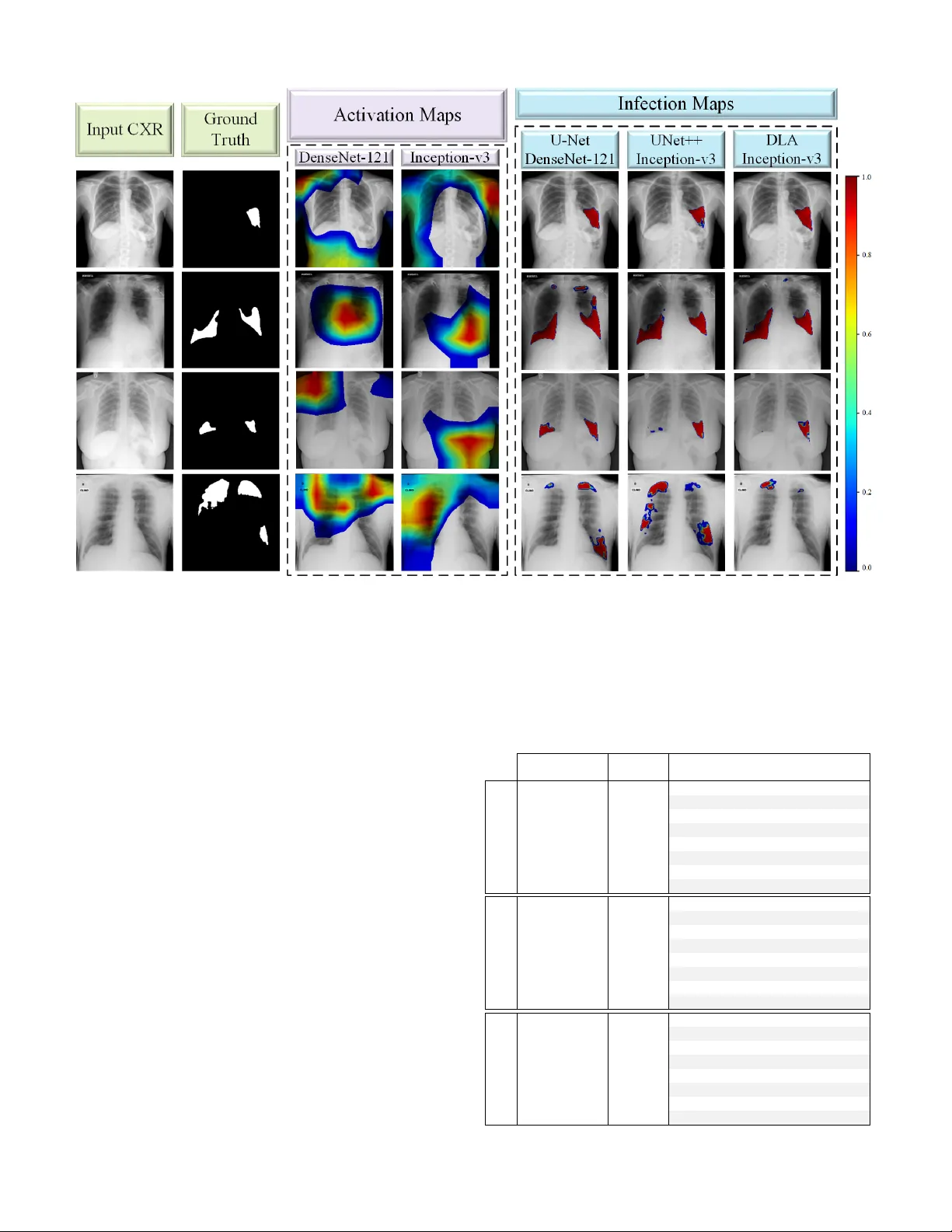
1 CO VID-19 Infection Map Generation and Detection from Chest X-Ray Images A ysen Degerli, Mete Ahishali, Mehmet Y amac, Serkan Kiranyaz, Muhammad E. H. Cho wdhury , Khalid Hameed, T ahir Hamid, Rashid Mazhar , and Moncef Gabbouj Abstract —Computer -aided diagnosis has become a necessity for accurate and immediate coronavirus disease 2019 (CO VID- 19) detection to aid treatment and pre vent the spr ead of the virus. Numerous studies ha ve proposed to use Deep Lear ning techniques for CO VID-19 diagnosis. Howe ver , they hav e used very limited chest X-ray (CXR) image repositories for evaluation with a small number , a few hundr eds, of CO VID-19 samples. Moreo ver , these methods can neither localize nor grade the severity of CO VID- 19 infection. F or this purpose, recent studies pr oposed to explore the activation maps of deep networks. However , they remain inaccurate for localizing the actual infestation making them unreliable for clinical use. This study proposes a novel method for the joint localization, severity grading, and detection of CO VID-19 from CXR images by generating the so-called infection maps . T o accomplish this, we have compiled the largest dataset with 119,316 CXR images including 2951 CO VID-19 samples, where the annotation of the ground-truth segmentation masks is performed on CXRs by a nov el collaborative human-machine approach. Furthermor e, we publicly release the first CXR dataset with the ground-truth segmentation masks of the CO VID-19 infected regions. A detailed set of experiments show that state- of-the-art segmentation networks can learn to localize CO VID- 19 infection with an F1-score of 83.20%, which is significantly superior to the acti vation maps created by the previous methods. Finally , the proposed approach achieved a COVID-19 detection performance with 94.96% sensitivity and 99.88% specificity . Index T erms —SARS-CoV -2, CO VID-19 Detection, COVID-19 Infection Segmentation, Deep Learning I . I N T RO D U C T I O N C OR ON A VIR US disease 2019 (CO VID-19) caused by sev ere acute respiratory syndrome Coronavirus-2 (SARs- CoV -2) w as first reported in December 2019 in W uhan, China. The highly infectious disease rapidly spread around the W orld with millions of positiv e cases. As a result, CO VID-19 w as declared as a pandemic by the W orld Health Organization in March 2020. The disease may lead to hospitalization, intuba- tion, intensi ve care, and ev en death, especially for the elderly [1], [2]. Naturally , reliable detection of the disease has the utmost importance. Ho we ver , the diagnosis of CO VID-19 is not straight-forward since its symptoms, such as cough, fev er , A ysen Degerli, Mete Ahishali, Mehmet Y amac, and Moncef Gabbouj are with the Faculty of Information T echnology and Communication Sciences, T ampere University , T ampere, Finland (e-mail: name.surname@tuni.fi). Serkan Kiranyaz and Muhammad E. H. Cho wdhury are with the De- partment of Electrical Engineering, Qatar University , Doha, Qatar (e-mail: mkiranyaz@qu.edu.qa and mchowdhury@qu.edu.qa). Khalid Hameed is an MD in Reem Medical Center, Doha, Qatar (e-mail: dr .khalid@reemmedicalcenter .com). T ahir Hamid is a consultant cardiologist in Hamad Medical Corporation Hospital and with W eill Cornell Medicine - Qatar , Doha, Qatar . Rashid Mazhar is an MD in Hamad Medical Corporation Hospital, Doha, Qatar . Fig. 1: The CO VID-19 sample CXR images, their correspond- ing ground-truth segmentation masks which are annotated by the collaborativ e human-machine approach, and the generated infection maps from the state-of-the-art segmentation models. breathlessness, and diarrhea are generally indistinguishable from other viral infections [3], [4]. The diagnostic tools to detect CO VID-19 are currently rev erse transcription of polymerase chain reaction (R T -PCR) assays and chest imaging techniques, such as Computed T o- mography (CT) and X-ray imaging. Primarily , R T -PCR has become the gold standard in the diagnosis of CO VID-19 [5], [6]. Howe ver , R T -PCR arrays hav e a high false alarm rate which may be caused by the virus mutations in the SARS-CoV -2 genome, sample contamination, or damage to the sample acquired from the patient [7], [8]. In f act, it is shown in hospitalized patients that R T -PCR sensiti vity is low and the test results are highly unstable [6], [9]–[11]. Therefore, it is recommended to perform chest CT imaging initially on the suspected CO VID-19 cases [12], since it is a more reliable clinical tool in the diagnosis with higher 2 sensitivity compared to R T -PCR. Hence, sev eral studies [12]– [14] suggest performing CT on the neg ativ e R T -PCR findings of the suspected cases. Howe ver , there are sev eral limitations of CT scans. Their sensitivity is limited in the early CO VID- 19 phase groups [15], and they are limited to recognize only specific viruses [16], slow in image acquisition, and costly . On the other hand, X-ray imaging is faster , cheaper , and less harmful to the body in terms of radiation exposure compared to CT [17], [18]. Moreo ver , unlike CT devices, X-ray de vices are easily accessible; hence, reducing the risk of CO VID- 19 contamination during the imaging process [19]. Currently , chest X-ray (CXR) imaging is widely used as an assistiv e tool in CO VID-19 prognosis, and it is reported to ha ve a potential diagnosis capability in recent studies [20]. In order to automate CO VID-19 detection/recognition from CXR images, many studies [17], [21]–[29] have proposed to use deep Conv olutional Neural Networks (CNNs). Howe ver , the main limitation of these studies is that the data is scarce for the target CO VID-19 class. Such a limited amount of data degrades the learning performance of the deep networks. T wo recent studies [30] and [31] hav e addressed this drawback with a compact network structure and achie v ed the state- of-the-art detection performance over the benchmark QaT a- CO V19 (initial version) and Early-QaT a-CO V19 datasets that consist of 462 and 175 CO VID-19 CXR images, respectiv ely . Although these datasets were the largest available at that time, such a limited number of CO VID-19 samples raises robustness and reliability issues for the proposed methods in general. Moreov er , all these previous machine learning solutions with X-ray imaging remain limited to only CO VID-19 detec- tion. Howe v er , as stated by Shi [32], CO VID-19 pneumonia screening is important for ev aluating the status of the patient and treatment. Therefore, along with the detection, CO VID- 19 related infection localization is another crucial problem. Hence, se v eral studies [33]–[35] produced activ ation maps that are generated from different Deep Learning (DL) models trained for CO VID-19 detection (classification) task to localize CO VID-19 infection in the lungs. Infection localization has two vital objectiv es: an accurate assessment of the infection location and the sev erity of the disease. Howe v er , the results of pre vious studies sho w that the acti v ation maps generated inherently from the underlying DL network may fail to accom- plish both objecti ves, that is, irrelev ant locations with biased sev erity grading appeared in many cases. T o overcome these problems, two studies [36], [37] proposed to perform lung segmentation as the first step in their approaches. This way , they hav e narrowed the region of interest down to the regions of lungs to increase the reliability of their methods. Overall, until this study , screening CO VID-19 infection from such activ ation maps produced by classification networks was the only option for the localization due to the absence of ground- truth of the datasets av ailable in the literature. Many studies [32], [36], [38]–[40] have CO VID-19 infection ground-truths for CT images; howe v er , ground-truth segmentation masks for CXR images are non-existent. In this study , in order to overcome the aforementioned limitations and drawbacks, first, the benchmark dataset QaT a- CO V19 proposed by the researchers of Qatar Uni versity and T ampere Uni v ersity in [30] and [31] is extended to include 2951 CO VID-19 samples. This ne w dataset is 3 - 20 times lar ger than those used in earlier studies. The extended benchmark dataset, QaT a-CO V19 with around 120 K CXR images, is not only the largest e v er composed dataset, but it is the first dataset that has the ground-truth segmentation masks for CO VID-19 infection regions, as some samples are sho wn in Fig. 1. A crucial property of QaT a-CO V19 dataset is that it contains CXRs with other (non-CO VID-19) infections and anomalies such as pneumonia and pulmonary edema, both of which exhibit high visual similarity to CO VID-19 infection in the lungs. Therefore, this is significantly more challenging task than distinguishing CO VID-19 from the normal (healthy) cases as almost all studies in the literature did. T o obtain the ground-truth segmentation masks for the CO VID-19 infected re gions, a human-machine collaborative approach is introduced. The objectiv e is to significantly reduce the human labor and thus to speed up and also to improve the segmentation masks because when they are drawn solely by medical doctors (MDs), human error due to limited perception, hand-crafting, and subjectivity will deteriorate the ov erall quality . This is an iterati v e process, where MDs initiate the segmentation by ”manually-drawn” segmentation masks for a subset of CXR images. Then, the trained se gmentation networks over this subset generate their own ”competing” masks and the MDs are asked to compare them pair-wise (initial manual segmentation vs. machine-segmented masks) for each patient. Such a verification improv es the quality of the generated masks as well as the (follo wing) training runs. Over the best masks selected by experts, the networks are trained again this time over a lar ger set (or e ven perhaps ov er the entire dataset), and among the masks generated by the networks, the best masks are selected by the MDs. This human-machine collaboration process continues until the MDs are fully satisfied, i.e., a satisfactory mask can be found among the masks generated by the networks for all CXR images in the dataset. In this study , we show that ev en with two stages (iterations), highly superior infection maps can be obtained using which an elegant CO VID-19 detection performance can be achiev ed. The rest of the paper is organized as follows. In Section II-A, we introduce the benchmark QaT a-CO V19 dataset. Our nov el human-machine collaborativ e approach for the ground- truth annotation is explained in Section II-B. Ne xt, the details of CO VID-19 infected region se gmentation, and the infection map generation and CO VID-19 detection are presented in Sections II-C and II-D, respectiv ely 1 . The experimental setup and results with the benchmark dataset are reported in Section III-A and III-B, respectiv ely . Finally , we conclude the paper in Section IV. I I . M A T E R I A L S A N D M E T H O D O L O G Y The proposed approach in this study is composed of three main phases: 1) training the state-of-the-art deep models for 1 The liv e demo of the proposed approach is implemented on http://qatacov .live/ 3 Fig. 2: The pipeline of the proposed approach has three stages: CO VID-19 infected region segmentation, infection map generation, and CO VID-19 detection. The CXR image is the input to the trained E-D CNN and the network’ s probabilistic prediction is used to generate infection maps. The generated infection maps are used for CO VID-19 detection. CO VID-19 infected region segmentation using the ground- truth segmentation masks, 2) infection map generation from the trained segmentation networks, and 3) CO VID-19 detec- tion as it can be depicted in Fig. 2. In this section, we first detail the creation of the benchmark QaT a-CO V19 dataset. Then, the proposed approach for collaborative human-machine ground-truth generation is introduced. A. The Benchmark QaT a-CO V19 Dataset The researchers of Qatar Uni versity and T ampere Uni- versity hav e compiled the largest CO VID-19 dataset up to date with nearly 120 K CXR images: QaT a-CO V19 including 2951 CO VID-19 CXRs. T o create QaT a-CO V19, we ha ve utilized sev eral publicly av ailable, scattered, and different for- mat datasets and repositories. Therefore, the collected images from the datasets had some duplicate, over -e xposed and low- quality images that were identified and remov ed in the pre- processing stage. Consequently , the CO VID-19 CXRs are from Fig. 3: The CO VID-19 CXR samples from the benchmark QaT a-CO V19 dataset. different publicly a v ailable sources resulting in high intra- class dissimilarity as depicted in Fig. 3. The image sources of CO VID-19 and control group CXRs are detailed as follows: CO VID-19 CXRs: BIMCV -CO VID19+ [41] is the largest publicly av ailable dataset with 2473 CO VID-19 positi ve CXR images. The CXR images of BIMCV -CO VID19+ dataset were recorded with computed radiography (CR) and digital X-ray (DX) machines. Hannover Medical School and Institute for Diagnostic and Interventional Radiology [42] released 183 CXR images of CO VID-19 patients. A total of 959 CXR images are from public repositories: Italian Society of Medical and Interventional Radiology (SIRM), GitHub, and Kaggle [37], [43]–[46]. As mentioned earlier , any duplication and low- quality images are remo ved since CO VID-19 CXR images are collected from dif ferent public datasets and repositories. In this study , a total of 2951 CO VID-19 CXRs are gathered from the aforementioned datasets. Therefore, CO VID-19 CXRs are of different age, group, gender , and ethnicity . Control Group CXRs: In this study , we have considered two control groups in the e xperimental ev aluation. Group- I consists of only normal (healthy) CXRs with a smaller number of images compared to the second group. RSN A pneumonia detection challenge dataset [47] is comprised of about 29 . 7 K CXR images, where 8851 images are normal. All CXRs in the dataset are in DICOM format, a popularly used format for medical imaging. Padchest dataset [48] consists of 160 , 868 CXR images from 67 , 625 patients, where 37 , 871 images are from normal class. The images are ev aluated and reported by radiologists at Hospital Sun Juan in Spain during 2009 − 2017 . The dataset includes six dif ferent position views of CXR and additional information regarding image acquisition and patient demography . Paul Mooney [49] has released an X-ray dataset of 5863 CXR images from a total of 5856 patients, where 1583 images are from normal class. The data is collected from pediatric patients aging one to fiv e years old at Guangzhou W omen and Children’ s Medical Center , Guangzhou. The dataset in [50] consists of 7470 CXR images and the corresponding radiologist reports from the Indiana Network for P atient Care, where a total of 1343 frontal 4 Fig. 4: The two stages of the human-machine collaborativ e approach. Stage I: A subset of CXR images with manually drawn segmentation masks are used to train three different deep networks in a 5-fold cross-validation scheme. The manually drawn ground-truth (a), and the three predictions (b, c, d) are blindly shown to MDs, and they select the best ground-truth mask. Stage II: Fiv e deep networks are trained over the best segmentation masks selected. Then, they are used to produce the segmentation masks for the rest of the CXR dataset (a, b, c, d, e), which are shown to MDs. CXR samples are labeled as normal. In [51], there are 80 normal CXRs from the tuberculosis control program of the Department of Health and Human Services of Montgomery County and 326 normal CXRs from Shenzhen Hospital. In this study , a total of 12 , 544 normal CXRs are included in con- trol Group-I from the aforementioned datasets. On the other hand, Group-II consists of 116 , 365 CXRs from 15 different classes. ChestX-ray14 [52] consists of 112 , 120 CXRs with normal and 14 different thoracic disease images, which are atelectasis, cardiomegaly , ef fusion, infiltration, mass, nodule, pneumonia, pneumothorax, consolidation, edema, emphysema, fibrosis, PT , hernia, and normal (no findings). Additionally , from the pediatric patients [49], 2760 bacterial and 1485 viral pneumonia CXRs are included in Group-II. B. Collaborative Human-Machine Gr ound-T ruth Annotation Recent de velopments in the machine and deep learning techniques led to state-of-the-art performance in many com- puter vision (CV) tasks, such as image classification, object detection, and image segmentation. Howe v er , supervised DL methods require a huge amount of annotated data. Otherwise, the limited amount of data de grades the performance of the deep network structures since their generalization capability depends on the av ailability of large datasets. Nevertheless, to produce ground-truth segmentation masks, pixel-accurate image segmentation by human experts can be a cumbersome and highly subjectiv e task ev en for moderate size datasets. In order to o vercome this challenge, in this study , we propose a no vel collaborati v e human-machine approach to accurately produce the ground-truth se gmentation masks for infected regions directly from the CXR images. The proposed approach is performed in two main stages. First, a group of expert MDs manually segment the infected regions of a subset of ( 500 in our case) CXR images. Then, se veral se gmentation networks that are inspired by the U-Net [53] structure with a 5-fold cross-v alidation scheme, are trained o ver the initial ground-truth masks. For each fold, the segmentation masks of the test samples are predicted by the networks. The network predicted masks along with the initial (MD drawn) ground- truth masks, and original CXR image are assessed by the MDs, and the best segmentation mask among them is selected. Steps of Stage-I are illustrated in Fig. 4 (top). At the end of the first stage, collaboratively annotated ground-truth masks for the subset of CXR images are formed, and they are obviously superior to the initial manually drawn masks since the y are selected by the MDs. An interesting observation in this stage was that MDs preferred the machine-generated masks over the manually drawn masks in the first stage in three out of five cases. In the second stage fiv e deep networks, inspired by U-Net [53], UNet++ [54], and DLA [55] architectures are trained ov er the collaborativ e masks, which were formed in Stage-I. The trained segmentation networks are used to predict the seg- mentation masks of the rest of the data, which is around 2400 unannotated CO VID-19 images. Among the fiv e predictions, the expert MDs select the best one as the ground-truth or deny all if none was found successful. For the latter case, MDs were asked to draw the ground-truth masks manually . Howe ver , 5 we notice that this was indeed a minority case that included less than 5 % of unannotated data. The steps of Stage-II are shown in Fig. 4 (bottom). As a result, the ground-truth masks for 2951 CO VID-19 CXR images are gathered to construct the benchmark QaT a-CO V19 dataset. The proposed approach does not only sav e v aluable human labor time, but it also improv es the quality and reliability of the masks by reducing the subjectivity with Stage-II verification step. C. CO VID-19 Infected Re gion Se gmentation Segmentation of CO VID-19 infection is the first step of our proposed approach as depicted in Fig. 2. Once the ground- truth annotation for QaT a-CO V19 benchmark dataset is formed as e xplained in the previous section, we perform infected region se gmentation extensi v ely with 24 different netw ork configurations. W e ha ve used three dif ferent segmentation models: U-Net, UNet++ and DLA, with four different encoder structures: CheXNet, DenseNet-121, Inception-v3 and ResNet- 50, and frozen & not frozen encoder weight configurations. 1) Se gmentation Models: W e have tried distinct segmenta- tion model structures starting from shallo w to deep structures with varied configurations as follows: • U-Net [53] is an outperforming netw ork for medical image segmentation applications with a u-shaped archi- tecture as the encoder part is symmetric with respect to its decoder part. Therefore, this unique decoder structure with many feature channels allows the network to carry the information through its latest layers. • UNet++ [54] has further dev eloped the decoder structure of U-Net by connecting the encoder to the decoder with the nested dense con volutional blocks. This way , the bridge between the encoder and decoder parts are more firmly knit; thus, the information can be transferred to its final layers more intensively compared to the classic U-Net. • DLA [55] in vestig ates the connecting bridges between the encoder and decoder , and proposes a way to fuse the semantic and spatial information with dense layers, which are progressively aggregated by iterati ve merging to deeper and larger scales. 2) Encoder Selections for Se gmentation Models: In this study , we use sev eral deep CNNs to form the encoder part of the above-mentioned segmentation models as follows: • DenseNet-121 [56] is a deep network with 121 layers, each with additional input nodes connecting all the layers directly with each other . Therefore, the maximum infor- mation flow through the network is satisfied. • CheXNet [57] is based on the architecture of DenseNet- 121, which is trained over the ChestX-ray14 dataset [52] to detect pneumonia cases from CXR images. In [57], DenseNet-121 is initialized with the ImageNet weights and fine-tuned ov er 100 K CXR images resulting from the state-of-the-art results on the ChestX-ray14 dataset with a better performance compared to the conclusions of radiologists. • Inception-v3 [58] achiev es state-of-the-art results with much less computational complexity compared to its deep competitors by factorizing the con volutions and pruning the dimensions inside the network. Despite the less complexity , it preserves a higher performance. • ResNet-50 [59] introduces a deep residual learning framew ork that forces the desired mapping of the input to a residual mapping. It is possible to achiev e this goal by the shortcut connections on the stacked layers. These connections enable to merge the input and output of the stacked layers by addition operations; therefore, the problem of gradient vanishing is prev ented. W e perform transfer learning on the encoder side of the seg- mentation models by initializing the layers with the ImageNet weights, except for CheXNet which is pre-trained on the ChestX-ray14 dataset. W e tried two configurations, in the first we freeze the encoder layers while in the second, they are allowed to vary . 3) Hybrid Loss Function: In this study , we have performed training the se gmentation networks with a hybrid loss function by combining focal loss [60] with dice loss [61] to achiev e a better segmentation performance. W e use focal loss since CO VID-19 infected region segmentation is an imbalanced problem: the number of background pixels is superior to the foreground’ s. Let the ground-truth segmentation mask be Y , where each pixel class label is defined as y , and the network prediction as ˆ y . W e define the pixel class probabilities as for the positiv e class P ( y = 1) = p , and for the neg ati ve class P ( y = 0) = 1 − p . On the other hand, the network prediction probabilities are modeled by the logistic function using the sigmoid curve as, P ( ˆ y = 1) = 1 1 + e − z = q (1) P ( ˆ y = 0) = 1 − 1 1 + e − z = 1 − q (2) where z is some function of the input CXR image X . Then, we define the cross-entropy (CE) loss as follows: C E ( p, q ) = − p log q − (1 − p ) log (1 − q ) . (3) A common solution to address the class imbalance problem is to add a weighting factor α ∈ [0 , 1] for the positi ve class, and 1 − α for the negati ve class, which defines the balanced cross-entropy (BCE) loss as, B C E ( p, q ) = − α p log q − (1 − α )(1 − p ) log(1 − q ) . (4) In this way , the importance of positive and neg ati ve samples are balanced. Ho we ver , adding the α factor does not solve the issue for the lar ge class imbalance scenario. This is because the network cannot distinguish outliers (hard samples) and inliers (easy samples) with the BCE loss. T o overcome this dra wback, focal loss [60] proposes to set focusing parameter γ ≥ 0 in order to down-weight the loss of easy samples that occur with small errors; so that the model can be forced to learn hard negati v e samples. The focal (F) loss is defined as, F ( p, q ) = − α (1 − q ) γ p log q − (1 − α ) q γ (1 − p ) log (1 − q ) . (5) where F loss is equiv alent to BCE loss when γ = 0 . In our experimental setup, we use the default setting as α = 0 . 25 , and 6 γ = 2 for all the networks. T o achiev e a good segmentation performance, we combined focal loss with dice loss, which is based on the dice coefficient (DC) defined as follows: D C = 2 | Y ∩ ˆ Y | | Y | ∪ | ˆ Y | (6) where ˆ Y is the predicted segmentation mask of the network. Hence, the DC can be interpreted as a dice (D) loss as follows: D ( p, q ) = 1 − 2 P p h,w q h,w P p h,w + P q h,w (7) where h and w are the height and width of the ground-truth and prediction masks Y and ˆ Y , respecti v ely . Finally , we combined D and F losses by summation to achie ve the so-called hybrid loss function for the segmentation networks. D. Infection Map Generation and CO VID-19 Detection Having the training set of CO VID-19 CXR images via the collaborativ e human-machine approach e xplained in Section II-A, we train the aforementioned segmentation networks to produce infection maps. After training the segmentation networks, we feed each test CXR sample X into the trained network. Then, we obtain the network prediction mask ˆ Y , which is used to generate an infection map that is a measure of infected region probabilities on the input X . Each pixel in ˆ Y is defined as ˆ Y h , w ∈ [0 , 1] , where h and w represent the size of the image. W e then apply an RGB-based color transform, i.e., the jet color scale to obtain the RGB version of the prediction mask, ˆ Y R,G,B as sho wn in Fig. 5 for a pseudo- colored probability measure visualization. The infection map is generated as a reflection of the network prediction ˆ Y R,G,B onto the CXR image X . Hence, for visualization, we form the imposed image by concatenating the hue and saturation components of ˆ Y H,S,V , and value component of X H,S,V . Fi- nally , the imposed image is con v erted back to RGB domain. In the infection map, we do not show the pixels/regions with zero probabilities for a better visualization effect. This way , the infected regions, where ˆ Y > 0 are shown translucent as in Fig 5. Along with the infection map generation, which already provides localization and segmentation of CO VID-19 infec- tion, CO VID-19 detection can easily be performed using the proposed approach. The detection of CO VID-19 is performed based on the predictions of the trained segmentation networks. Accordingly , a test sample is classified as CO VID-19 class if ˆ Y ≥ 0 . 5 at any pixel location. I I I . E X P E R I M E N T A L R E S U LT S In this section, first, the experimental setup is presented. Then, both numerical and visual results are reported with an extensi v e set of comparative ev aluations over the benchmark QaT a-CO V19 dataset. Finally , visual comparativ e ev aluations are presented between the infection maps and the acti v ation maps extracted from state-of-the-art deep models. Fig. 5: The three CO VID-19 CXR test samples, X with the corresponding ground-truth masks, Y . The color-coded network predictions, ˆ Y R , G , B are reflected translucent onto the X to generate an infection map on the lungs, where ˆ Y > 0 . A. Experimental Setup Quantitativ e ev aluations for the proposed approach are per- formed for both CO VID-19 infected region segmentation and CO VID-19 detection. CO VID-19 infected region segmentation is e v aluated on a pix el-le v el, where we consider the fore ground (infected re gion) as the positiv e class, and background as the negati v e class. For CO VID-19 detection, the performance is computed per CXR sample, and we consider CO VID-19 as the positi ve class and the control group as the negati ve class. Overall, elements of the confusion matrix are formed as follows: true positi ve (TP): the number of correctly detected positiv e class members, true negati v e (TN): the number of correctly detected negati v e class samples, false positive (FP): the number of misclassified ne gati ve class members, and false negati v e (FN): the number of misclassified positi ve class samples. The standard performance ev aluation metrics are defined as follows: S ensitiv ity = T P T P + F N (8) where sensitivity (or Recall) is the rate of correctly detected positiv e samples in the positiv e class samples, S pecif icity = T N T N + F P (9) where specificity is the ratio of accurately detected negati ve class samples to all negati v e class samples, P recision = T P T P + F P (10) where precision is the rate of correctly classified positi v e class samples among all the members classified as positiv e samples, Accur acy = T P + T N T P + T N + F P + F N (11) 7 T ABLE I: A verage performance metrics (%) for CO VID-19 infected r egion se gmentation computed on the Group-I test (unseen) set from 5 -folds with three state-of-the-art segmentation models, four encoder architectures, and weight initializations. The initialized encoder layers are set to fr ozen ( 3 ) and not frozen ( 7 ) states during the in vestigation. Model Encoder Encoder Layers Sensitivity Specificity Precision F1-Score F2-Score Accuracy A UC U-Net CheXNet 3 81 . 20 ± 1 . 6 × 10 − 4 99 . 55 ± 5 × 10 − 6 83 . 78 ± 2 . 6 × 10 − 5 82 . 47 ± 2 . 7 × 10 − 5 81 . 70 ± 2 . 7 × 10 − 5 99 . 03 ± 6 . 9 × 10 − 6 99 . 19 ± 6 . 3 × 10 − 6 CheXNet 7 82 . 23 ± 1 . 6 × 10 − 4 99 . 56 ± 5 × 10 − 6 84 . 54 ± 2 . 5 × 10 − 5 83 . 34 ± 2 . 6 × 10 − 5 82 . 66 ± 2 . 7 × 10 − 5 99 . 08 ± 6 . 7 × 10 − 6 99 . 18 ± 6 . 3 × 10 − 6 DenseNet-121 3 82 . 29 ± 1 . 6 × 10 − 4 99 . 61 ± 4 × 10 − 6 86 . 02 ± 2 . 4 × 10 − 5 84 . 11 ± 2 . 6 × 10 − 5 83 . 01 ± 2 . 6 × 10 − 5 99 . 13 ± 6 . 5 × 10 − 6 99.35 ± 5 . 6 × 10 − 6 DenseNet-121 7 84.00 ± 1 . 5 × 10 − 4 99 . 66 ± 4 × 10 − 6 87 . 77 ± 2 . 3 × 10 − 5 85.81 ± 2 . 5 × 10 − 5 84.71 ± 2 . 5 × 10 − 5 99.22 ± 6 . 2 × 10 − 6 99 . 19 ± 6 . 3 × 10 − 6 Inception-v3 3 80 . 42 ± 1 . 7 × 10 − 4 99 . 59 ± 5 × 10 − 6 84 . 94 ± 2 . 5 × 10 − 5 82 . 62 ± 2 . 7 × 10 − 5 81 . 28 ± 2 . 7 × 10 − 5 99 . 05 ± 6 . 8 × 10 − 6 99 . 20 ± 6 . 3 × 10 − 6 Inception-v3 7 82 . 34 ± 1 . 6 × 10 − 4 99.70 ± 4 × 10 − 6 88.87 ± 2 . 2 × 10 − 5 85 . 43 ± 2 . 5 × 10 − 5 83 . 54 ± 2 . 6 × 10 − 5 99 . 21 ± 6 . 2 × 10 − 6 98 . 82 ± 7 . 6 × 10 − 6 ResNet-50 3 81 . 43 ± 1 . 6 × 10 − 4 99 . 62 ± 4 × 10 − 6 86 . 07 ± 2 . 4 × 10 − 5 83 . 67 ± 2 . 6 × 10 − 5 82 . 31 ± 2 . 6 × 10 − 5 99 . 11 ± 6 . 6 × 10 − 6 99 . 30 ± 5 . 9 × 10 − 6 ResNet-50 7 79 . 90 ± 1 . 7 × 10 − 4 99.70 ± 4 × 10 − 6 88 . 64 ± 2 . 2 × 10 − 5 83 . 89 ± 2 . 6 × 10 − 5 81 . 43 ± 2 . 7 × 10 − 5 99 . 15 ± 6 . 5 × 10 − 6 98 . 98 ± 7 . 1 × 10 − 6 UNet++ CheXNet 3 80 . 29 ± 1 . 7 × 10 − 4 99 . 59 ± 5 × 10 − 6 85 . 19 ± 2 . 5 × 10 − 5 82 . 64 ± 2 . 7 × 10 − 5 81 . 21 ± 2 . 7 × 10 − 5 99 . 05 ± 6 . 8 × 10 − 6 99 . 01 ± 7 × 10 − 6 CheXNet 7 81 . 45 ± 1 . 6 × 10 − 4 99 . 60 ± 5 × 10 − 6 85 . 60 ± 2 . 5 × 10 − 5 83 . 47 ± 2 . 6 × 10 − 5 82 . 24 ± 2 . 7 × 10 − 5 99 . 09 ± 6 . 7 × 10 − 6 99 . 01 ± 7 × 10 − 6 DenseNet-121 3 82 . 38 ± 1 . 6 × 10 − 4 99 . 61 ± 4 × 10 − 6 85 . 99 ± 2 . 4 × 10 − 5 84 . 14 ± 2 . 6 × 10 − 5 83 . 08 ± 2 . 6 × 10 − 5 99 . 13 ± 6 . 5 × 10 − 6 99 . 19 ± 6 . 3 × 10 − 6 DenseNet-121 7 82 . 36 ± 1 . 6 × 10 − 4 99.68 ± 4 × 10 − 6 88.07 ± 2 . 3 × 10 − 5 85 . 08 ± 2 . 5 × 10 − 5 83 . 42 ± 2 . 6 × 10 − 5 99 . 19 ± 6 . 3 × 10 − 6 99.30 ± 5 . 9 × 10 − 6 Inception-v3 3 82 . 87 ± 1 . 6 × 10 − 4 99 . 57 ± 5 × 10 − 6 84 . 83 ± 2 . 5 × 10 − 5 83 . 81 ± 2 . 6 × 10 − 5 83 . 24 ± 2 . 6 × 10 − 5 99 . 10 ± 6 . 6 × 10 − 6 99 . 21 ± 6 . 2 × 10 − 6 Inception-v3 7 83.49 ± 1 . 6 × 10 − 4 99 . 66 ± 4 × 10 − 6 87 . 60 ± 2 . 3 × 10 − 5 85.45 ± 2 . 5 × 10 − 5 84.22 ± 2 . 6 × 10 − 5 99.20 ± 6 . 3 × 10 − 6 99 . 18 ± 6 . 3 × 10 − 6 ResNet-50 3 82 . 07 ± 1 . 6 × 10 − 4 99 . 59 ± 5 × 10 − 6 85 . 41 ± 2 . 5 × 10 − 5 83 . 71 ± 2 . 6 × 10 − 5 82 . 72 ± 2 . 7 × 10 − 5 99 . 10 ± 6 . 6 × 10 − 6 99 . 15 ± 6 . 5 × 10 − 6 ResNet-50 7 82 . 64 ± 1 . 6 × 10 − 4 99 . 62 ± 4 × 10 − 6 86 . 52 ± 2 . 4 × 10 − 5 84 . 45 ± 2 . 5 × 10 − 5 83 . 33 ± 2 . 6 × 10 − 5 99 . 14 ± 6 . 5 × 10 − 6 99 . 27 ± 6 × 10 − 6 DLA CheXNet 3 79 . 99 ± 1 . 7 × 10 − 4 99 . 61 ± 4 × 10 − 6 85 . 57 ± 2 . 5 × 10 − 5 82 . 66 ± 2 . 7 × 10 − 5 81 . 04 ± 2 . 8 × 10 − 5 99 . 06 ± 6 . 8 × 10 − 6 99 . 12 ± 6 . 6 × 10 − 6 CheXNet 7 82 . 84 ± 1 . 6 × 10 − 4 99 . 56 ± 5 × 10 − 6 84 . 63 ± 2 . 5 × 10 − 5 83 . 71 ± 2 . 6 × 10 − 5 83 . 19 ± 2 . 6 × 10 − 5 99 . 09 ± 6 . 7 × 10 − 6 99 . 17 ± 6 . 4 × 10 − 6 DenseNet-121 3 82 . 48 ± 1 . 6 × 10 − 4 99 . 62 ± 4 × 10 − 6 86 . 40 ± 2 . 4 × 10 − 5 84 . 36 ± 2 . 6 × 10 − 5 83 . 21 ± 2 . 6 × 10 − 5 99 . 14 ± 6 . 5 × 10 − 6 99 . 16 ± 6 . 4 × 10 − 6 DenseNet-121 7 82 . 84 ± 1 . 6 × 10 − 4 99 . 56 ± 5 × 10 − 6 84 . 63 ± 2 . 5 × 10 − 5 83 . 71 ± 2 . 6 × 10 − 5 83 . 19 ± 2 . 6 × 10 − 5 99 . 09 ± 6 . 7 × 10 − 6 99 . 17 ± 6 . 4 × 10 − 6 Inception-v3 3 80 . 28 ± 1 . 7 × 10 − 4 99 . 63 ± 4 × 10 − 6 86 . 43 ± 2 . 4 × 10 − 5 83 . 19 ± 2 . 6 × 10 − 5 81 . 41 ± 2 . 7 × 10 − 5 99 . 09 ± 6 . 7 × 10 − 6 99 . 02 ± 6 . 9 × 10 − 6 Inception-v3 7 83.44 ± 1 . 6 × 10 − 4 99.68 ± 4 × 10 − 6 88.18 ± 2 . 3 × 10 − 5 85.73 ± 2 . 5 × 10 − 5 84.34 ± 2 . 6 × 10 − 5 99.22 ± 6 . 2 × 10 − 6 99.29 ± 5 . 9 × 10 − 6 ResNet-50 3 81 . 26 ± 1 . 6 × 10 − 4 99 . 63 ± 4 × 10 − 6 86 . 48 ± 2 . 4 × 10 − 5 83 . 78 ± 2 . 6 × 10 − 5 82 . 25 ± 2 . 7 × 10 − 5 99 . 12 ± 6 . 6 × 10 − 6 99 . 08 ± 6 . 7 × 10 − 6 ResNet-50 7 82 . 07 ± 1 . 6 × 10 − 4 99 . 65 ± 4 × 10 − 6 86 . 99 ± 2 . 4 × 10 − 5 84 . 45 ± 2 . 5 × 10 − 5 83 . 00 ± 2 . 6 × 10 − 5 99 . 15 ± 6 . 5 × 10 − 6 99 . 31 ± 5 . 8 × 10 − 6 where accuracy is the ratio of correctly classified elements among all the data, F ( β ) = (1 + β 2 ) ( P recision × S ensitiv ity ) β 2 × P r ecision + S ensitiv ity (12) where F -score is defined by the weighting parameter β . The F1 -Score is calculated with β = 1 , which is the harmonic av erage of precision and sensitivity . The F2 -score is calculated with β = 2 , which emphasizes FN minimization ov er FPs. The main objecti ve of both CO VID-19 segmentation and detection is to maximize sensitivity with a reasonable specificity in order to minimize FP CO VID-19 cases or pixels. Equiv alently , maximized F2 -score is targeted with an acceptable F1 -Score value. The performances with their 95 % confidence interval (CI) for both CO VID-19 infected region segmentation and detection are gi ven in T ables I and III, respecti v ely . The range of values can be calculated for each performance as follows: r = ± z p metr ic (1 − metric ) / N , (13) where z is the lev el of significance, metric is any perfor- mance e valuation metric, and N is the number of samples. Accordingly , z is set to 1 . 96 for 95 % CI. W e have implemented the deep networks with T ensorflow library [62] using Python on NV idia ® GeF orce R TX 2080 T i GPU card. F or training, Adam optimizer [63] is used with the default momentum parameters, β 1 = 0 . 9 and β 2 = 0 . 999 using the aforementioned hybrid loss function. The segmenta- tion networks are trained with 50 -epochs with a learning rate of α = 10 − 4 and a batch size of 32 . For comparing the computed infection maps, the activ ation maps are computed as follows: the encoder structures of the segmentation networks are trained for the classification task with a modification at the output layer by adding 2 -neurons for the number of total classes. The acti v ation maps e xtracted from the classification models are then compared with the infection maps of the segmentation models. The classification networks, CheXNet, DenseNet-121, Inception-v3 and ResNet-50 are fine-tuned using cate gorical cross-entrop y as loss function with 10 epochs and a learning rate of α = 10 − 5 , which is a sufficient setting to prev ent over -fitting, based on our previous study [31]. Other settings of the classifiers are kept the same with the segmentation models. B. Experimental Results The e xperiments are carried out for both CO VID-19 infected region segmentation and CO VID-19 detection. W e extensiv ely tested the benchmark QaT a-CO V19 dataset using three differ - ent state-of-the-art segmentation networks with four different encoder options for the initial dataset consisting of control Group-I. W e also in vestig ated the effect of frozen encoder weights on the performance. On the other hand, the leading model is selected and ev aluated on the extended dataset, which includes more negati ve samples with the control Group-II. 1) Gr oup-I Experiments: W e have ev aluated the networks in a stratified 5-fold cross-validation scheme with a ratio of 80% training to 20% test (unseen folds) ov er the benchmark QaT a-CO V19 dataset. The input CXR images are resized to 224 × 224 pixels. T able II sho ws the number of CXRs per fold in the dataset. Since the two classes are imbalanced, we hav e applied data augmentation in order to balance the classes. Therefore, CO VID-19 samples are augmented up to the same number of samples as the control Group-I in the training set for each fold. The data augmentation is performed using Image Data Generator in Keras: the CXR samples are augmented by randomly shifting them both vertically and horizontally by 10% and randomly rotating them in a range of 10 degrees. T ABLE II: Number of CXR samples in control Group-I per fold before and after data augmentation. Data Number of Samples T raining Samples Augmented T raining Samples T est Samples CO VID-19 2951 2361 10035 590 Group-I 12544 10035 10035 2509 T otal 15495 12396 20070 3099 8 T ABLE III: A verage CO VID-19 detection performance results (%) computed from 5 -folds over the Group-I test (unseen) set with three netw ork models, four encoder architectures, and weight initializations. The initialized encoder layers are set to fr ozen ( 3 ) and not frozen ( 7 ) states during the inv estigation. Encoder Encoder Layers Sensitivity Specificity Precision F1-Score F2-Score Accurac y U-Net CheXNet 3 97 . 56 ± 0 . 0056 91 . 10 ± 0 . 0050 72 . 07 ± 0 . 0071 82 . 90 ± 0 . 0059 91 . 11 ± 0 . 0045 92 . 33 ± 0 . 0042 CheXNet 7 97 . 97 ± 0 . 0051 92 . 74 ± 0 . 0045 76 . 04 ± 0 . 0067 85 . 62 ± 0 . 0055 92 . 62 ± 0 . 0041 93 . 73 ± 0 . 0038 DenseNet-121 3 98 . 07 ± 0 . 0050 94 . 66 ± 0 . 0039 81 . 20 ± 0 . 0062 88 . 84 ± 0 . 0050 94 . 16 ± 0 . 0037 95 . 31 ± 0 . 0033 DenseNet-121 7 98.37 ± 0 . 0046 98 . 05 ± 0 . 0024 92 . 25 ± 0 . 0042 95 . 21 ± 0 . 0034 97.08 ± 0 . 0027 98 . 12 ± 0 . 0021 Inception-v3 3 97 . 93 ± 0 . 0051 90 . 00 ± 0 . 0052 69 . 74 ± 0 . 0072 81 . 47 ± 0 . 0061 90 . 61 ± 0 . 0046 91 . 51 ± 0 . 0044 Inception-v3 7 97 . 22 ± 0 . 0059 98.37 ± 0 . 0022 93.33 ± 0 . 0039 95.24 ± 0 . 0034 96 . 42 ± 0 . 0029 98.15 ± 0 . 0021 ResNet-50 3 98 . 24 ± 0 . 0047 93 . 88 ± 0 . 0042 79 . 06 ± 0 . 0064 87 . 61 ± 0 . 0052 93 . 69 ± 0 . 0038 94 . 71 ± 0 . 0035 ResNet-50 7 96 . 37 ± 0 . 0067 97 . 82 ± 0 . 0026 91 . 21 ± 0 . 0045 93 . 72 ± 0 . 0038 95 . 30 ± 0 . 0033 97 . 54 ± 0 . 0024 UNet++ CheXNet 3 97 . 80 ± 0 . 0053 91 . 70 ± 0 . 0048 73 . 49 ± 0 . 0069 83 . 92 ± 0 . 0058 91 . 73 ± 0 . 0043 92 . 86 ± 0 . 0041 CheXNet 7 97 . 49 ± 0 . 0056 93 . 65 ± 0 . 0043 78 . 33 ± 0 . 0065 86 . 87 ± 0 . 0053 92 . 94 ± 0 . 0040 94 . 39 ± 0 . 0036 DenseNet-121 3 97 . 70 ± 0 . 0054 94 . 81 ± 0 . 0039 81 . 58 ± 0 . 0061 88 . 91 ± 0 . 0049 93 . 98 ± 0 . 0037 95 . 36 ± 0 . 0033 DenseNet-121 7 96 . 51 ± 0 . 0066 99.16 ± 0 . 0016 96.44 ± 0 . 0029 96.48 ± 0 . 0029 96.50 ± 0 . 0029 98.66 ± 0 . 0018 Inception-v3 3 98.31 ± 0 . 0047 90 . 54 ± 0 . 0051 70 . 96 ± 0 . 0071 82 . 43 ± 0 . 0060 91 . 27 ± 0 . 0044 92 . 02 ± 0 . 0043 Inception-v3 7 96 . 92 ± 0 . 0061 98 . 37 ± 0 . 0022 93 . 34 ± 0 . 0039 95 . 10 ± 0 . 0034 96 . 18 ± 0 . 0030 98 . 10 ± 0 . 0021 ResNet-50 3 97 . 80 ± 0 . 0053 93 . 39 ± 0 . 0043 77 . 69 ± 0 . 0066 86 . 59 ± 0 . 0054 92 . 98 ± 0 . 0040 94 . 23 ± 0 . 0037 ResNet-50 7 96 . 78 ± 0 . 0064 97 . 43 ± 0 . 0028 89 . 87 ± 0 . 0048 93 . 20 ± 0 . 0040 95 . 31 ± 0 . 0033 97 . 31 ± 0 . 0025 DLA CheXNet 3 97 . 46 ± 0 . 0057 92 . 47 ± 0 . 0046 75 . 27 ± 0 . 0068 84 . 94 ± 0 . 0056 92 . 03 ± 0 . 0043 93 . 42 ± 0 . 0039 CheXNet 7 97 . 32 ± 0 . 0058 94 . 93 ± 0 . 0038 81 . 87 ± 0 . 0061 88 . 93 ± 0 . 0049 93 . 78 ± 0 . 0038 95 . 39 ± 0 . 0033 DenseNet-121 3 97 . 36 ± 0 . 0058 95 . 66 ± 0 . 0036 84 . 08 ± 0 . 0058 90 . 23 ± 0 . 0047 94 . 38 ± 0 . 0036 95 . 99 ± 0 . 0031 DenseNet-121 7 97 . 09 ± 0 . 0061 99 . 07 ± 0 . 0017 96 . 08 ± 0 . 0031 96.58 ± 0 . 0029 96.88 ± 0 . 0027 98.69 ± 0 . 0018 Inception-v3 3 96 . 92 ± 0 . 0062 93 . 24 ± 0 . 0044 77 . 13 ± 0 . 0066 85 . 90 ± 0 . 0055 92 . 19 ± 0 . 0042 93 . 94 ± 0 . 0040 Inception-v3 7 96 . 71 ± 0 . 0064 99.13 ± 0 . 0016 96.32 ± 0 . 0030 96 . 52 ± 0 . 0029 96 . 63 ± 0 . 0028 98 . 67 ± 0 . 0018 ResNet-50 3 97.49 ± 0 . 0056 95 . 30 ± 0 . 0037 82 . 98 ± 0 . 0059 89 . 65 ± 0 . 0048 94 . 20 ± 0 . 0037 95 . 71 ± 0 . 0032 ResNet-50 7 96 . 17 ± 0 . 0069 98 . 15 ± 0 . 0024 92 . 44 ± 0 . 0042 94 . 27 ± 0 . 0037 95 . 40 ± 0 . 0033 97 . 77 ± 0 . 0023 After shifting and rotating the images, blank sections are filled using the nearest mode. The performance of the segmentation models for CO VID- 19 infected region segmentation are presented in T able I. Each model structure is e v aluated with two configurations: fr ozen and not fr ozen encoder layers. W e hav e used transfer learning on the encoder layers with ImageNet weights, except for the CheXNet model, which is pre-trained on the ChestX-ray14 dataset. The ev aluation of the models with frozen encoder layers is also important since this process can lead to a better con v ergence and improv ed performance. Howe v er , as the Fig. 6: The Precision-Recall curves of the three leading models all with the not frozen encoder layers setting. results show , better performance is obtained when the network continues to learn on the encoder layers as well. For each model, we have observed that two encoders: DenseNet-121 and Inception-v3 are the top-performing ones for the infected region segmentation task. The U-Net model with DenseNet- 121 encoder holds the leading performance by 84 % sensi- tivity , 85 . 81 % F1-Score, and 84 . 71 % F2-Score. DenseNet- 121 produces better results compared to other encoder types since it can preserve the information coming from earlier layers through the output by concatenating the feature maps from each dense layer . Howe v er , in the other se gmentation models, Inception-v3 outperforms the other encoder types. The presented segmentation performances are obtained by setting the threshold value to 0 . 5 to compute the segmentation mask from the network probabilities. The Precision-Recall curves are plotted in Fig. 6 by varying this threshold value. The performances of the segmentation models for CO VID- 19 detection are presented in T able III. All the models are ev aluated by stratified a 5-fold cross-v alidation scheme, and the table sho ws the a veraged results of these folds. The most crucial metric here is the sensitivity since missing any patient with CO VID-19 is critical. In fact, the results indicate the robustness of the model as the proposed approach can achiev e high sensitivity lev els of 98 . 37 % with a 97 . 08 % F2- Score. Additionally , the proposed approach achie ves an ele gant specificity of 99 . 16 %, indicating a significantly low false alarm rate. It can be observed from T able III that DenseNet- 121 encoder with the not frozen encoder layer setting gives the most promising results among the others. The confusion matrices, accumulated on each fold’ s test set, are presented in T able IV. The highest sensitivity in CO VID-19 detection is achie v ed by the U-Net DenseNet-121 model (T able IV a). Accordingly , the U-Net DenseNet-121 model only misses 48 9 T ABLE IV: Cumulative confusioFn matrices of CO VID-19 detection by the best performing U-Net and UNet++ models with DenseNet-121 encoder . (a) U-Net DenseNet-121 U-Net Predicted Group-I CO VID-19 Ground T ruth Group-I 12300 244 CO VID-19 48 2903 (b) UNet++ DenseNet-121 UNet++ Predicted Group-I CO VID-19 Ground T ruth Group-I 12439 105 CO VID-19 103 2848 CO VID-19 patients out of 2951 . On the other hand, the highest specificity is achieved by UNet++ DenseNet-121 model (T able IVb). The UNet++ model only misses a minor part of the control class with 105 samples out of 12544 . 2) Gr oup-II Experiments: W e ha ve selected the leading model from the Group-I e xperiments as U-Net with not frozen DenseNet-121 encoder setting. In Group-II experiments, we hav e gathered around 120 K CXRs. The CXRs from the ChestX-ray14 dataset [52] are already divided into train and test sets. Accordingly , we have randomly separated the train and test sets of CO VID-19, viral pneumonia, and bacterial pneumonia CXRs by keeping the same train/test ratio as in ChestX-ray14 [52]. T able V shows the number of training and test samples of the Group-II experiments. Additonally , we hav e applied augmentation to data except for ChestX-ray14 samples with the same set-up as in the Group-I experiments. In these experiments, we do not perform any cross-v alidation since ChestX-ray14 has predefined training and test sets. T ABLE V: Number of CXR samples in control Group-II before and after data augmentation. Data T raining Samples Augmented Augmented T raining Samples T est Samples CO VID-19 2078 3 10 , 000 873 Bacterial Pneumonia 2130 3 5000 630 ChestX-ray14 86 , 524 7 86 , 524 25 , 596 V iral Pneumonia 1146 3 5000 339 T otal 91,878 106,524 27,438 The performance of the U-Net model for CO VID-19 in- fected region segmentation and detection is presented in T a- ble VI. The model achie v ed a segmentation performance by 81 . 72 % sensitivity and 83 . 20 % F1-Score. In comparison to initial experiments with the control Group-I data, the model can still achie ve an elegant segmentation performance even with numerous samples in the test set. On the other hand, the CO VID-19 detection performance with 27 , 438 CXR images is very successful by 94 . 96 % sensitivity , 99 . 88 % specificity , and 96 . 40 % precision. This indicates a very lo w false alarm rate of only 0 . 12 %. T able VII shows the confusion matrix on the test set. Accordingly , the model only misses 44 CO VID-19 samples. In the control Group-II, only 31 CXR samples are T ABLE VI: CO VID-19 infected re gion segmentation and de- tection results (%) computed on the Group-II test set from the U-Net model with DenseNet-121 encoder . Performance Metrics Infected Region Segmentation Detection U-Net DenseNet-121 Sensitivity 81 . 72 94 . 96 Specificity 99 . 93 99 . 88 Precision 84 . 74 96 . 40 F1-Score 83 . 20 95 . 67 F2-Score 82 . 31 95 . 24 Accuracy 99 . 85 99 . 73 T ABLE VII: Cumulati v e confusion matrices of CO VID-19 detection by the best performing U-Net model with DenseNet- 121 encoder . U-Net Predicted Group-II CO VID-19 Ground T ruth Group-II 26 , 534 31 CO VID-19 44 829 missed, which is a minor section in 26 , 565 negati ve samples. The results show that the leading model is still robust on the extended data, where it consists of 15 different classes with 14 thoracic diseases and normal samples. C. Infection vs Activation Maps Sev eral studies [33]–[35] propose to localize CO VID-19 from CXRs by extracting acti v ation maps from the deep classification models trained for CO VID-19 detection. Despite the simplicity of the idea, there are many limitations of this ap- proach. First of all, without any infected re gion segmentation ground-truth masks, the network can only produce a rough localization, and the extracted acti v ation maps may entirely fail to localize CO VID-19 infection. In this study , we check the reliability of our proposed CO VID-19 detection approach by comparing it with DL mod- els trained for the classification task. In order to achiev e this objectiv e, we compare the infection map and acti v ation map of CXR images, which are generated from the segmentation and classification networks, respecti vely . Therefore, we hav e trained the encoder structures of the segmentation networks, which are CheXNet, DenseNet-121, Inception-v3, and ResNet- 50 to perform CO VID-19 classification task. W e have extracted activ ation maps from these trained models by the Gradient- weighted Class Acti v ation Mapping (Grad-CAM) approach proposed in [64]. The localization Grad-CAM L c Grad-CAM ∈ R h × w of height h and width w for class c is calculated by the gradient of m c before the softmax with respect to the con v olutional layer’ s feature maps A k as ∂ m c ∂ A k . The gradients are passed through from the global average pooling during back-propagation; α c k = 1 Z X i X j ∂ m c ∂ A k , (14) where α is the weight that shows the important feature map k from A for a target class c . Then, the linear combination is 10 Fig. 7: Sev eral CXR images with their corresponding ground-truth masks. The activ ation maps extracted from the classification models are presented in the middle block. The last block is the generated infection maps from the segmentation models. It is evident that the infection maps yield a superior localization of CO VID-19 infection compared to activ ation maps. performed following by ReLU to obtain the Grad-CAM; L c Grad-CAM = ReLU ( X k α c k A k ) . (15) Despite their elegant performance, acti v ation maps e xtracted from deep classification networks are not suitable for localiz- ing CO VID-19 infection as depicted in Fig 7. In fact, infections found by the activ ation maps are highly irrelev ant indicating false locations outside of the lung areas. On the other hand, infection maps can generate a highly accurate location with an elegant severity grading of CO VID-19 infection. The pro- posed infection maps can con v eniently be used by medical experts for an enhanced assessment of the disease. Real-time implementation of the infection maps will obviously speed up the detection process, can also monitor the progression of CO VID-19 infection in the lungs. D. Computational Complexity Analysis In this section, we present the computational times of the networks and their number of trainable & non-trainable parameters. T able VIII shows the elapsed time in milliseconds (ms) during the inference step for each network used in the experiments. The results in the table represent the running time per sample. It can be observed from the table that the U- Net model is the fastest among the others due to its shallow structure. The f astest network is U-Net Inception-v3 with T ABLE VIII: The number of trainable and non-trainable parameters of the models with their inference time (ms) per sample. The initialized encoder layers are set to frozen ( 3 ) or not frozen ( 7 ). Encoder Encoder Layers T rainable Non-T rainable T ime (ms) U-Net CheXNet 3 5 . 19 M 6 . 96 M 2 . 56 DenseNet-121 3 5 . 19 M 6 . 96 M 2 . 58 Inception-v3 3 8 . 15 M 21 . 79 M 2.53 ResNet-50 3 9 . 06 M 23 . 50 M 2 . 54 CheXNet 3 12 . 06 M 85 . 63 K 2 . 62 DenseNet-121 7 12 . 06 M 85 . 63 K 2 . 58 Inception-v3 7 29 . 9 M 36 . 42 K 2 . 61 ResNet-50 7 32 . 51 M 47 . 56 K 2 . 64 UNet++ CheXNet 3 7 . 53 M 6 . 96 M 5 . 17 DenseNet-121 3 7 . 53 M 6 . 96 M 5 . 10 Inception-v3 3 8 . 68 M 21 . 79 M 5 . 32 ResNet-50 3 10 . 88 M 23 . 51 M 5 . 58 CheXNet 7 14 . 40 M 88 . 45 K 5 . 24 DenseNet-121 7 14 . 40 M 88 . 45 K 5 . 25 Inception-v3 7 30 . 43 M 39 . 23 K 5 . 32 ResNet-50 7 34 . 34 M 50 . 37 K 5 . 46 DLA CheXNet 3 6 . 27 M 6 . 96 M 4 . 65 DenseNet-121 3 6 . 27 M 6 . 96 M 4 . 63 Inception-v3 3 7 . 20 M 21 . 79 M 4 . 70 ResNet-50 3 8 . 74 M 23 . 51 M 4 . 90 CheXNet 7 13 . 15 M 88 . 45 K 4 . 63 DenseNet-121 7 13 . 15 M 88 . 45 K 4 . 65 Inception-v3 7 28 . 96 M 39 . 23 K 4 . 72 ResNet-50 7 32 . 2 M 50 . 37 K 4 . 90 11 frozen encoder layers taking up 2 . 53 ms. On the other hand, the slowest model is UNet++ structure since it has the largest number of trainable parameters. The most computationally demanding model is UNet++ ResNet-50 with frozen encoder layers, which takes 5 . 58 ms. W e, therefore, conclude that all models can be used as real-time clinical applications. I V . C O N C L U S I O N S The immediate and accurate detection of highly infectious CO VID-19 plays a vital role in prev enting the spread of the virus. In this study , we used CXR images since X-ray imaging is cheaper , easily accessible, and faster than the conv entional methods commonly used such as R T -PCR and CT . As a major contribution, the largest CXR dataset, QaT a-CO V19, which consists of 2951 CO VID-19, and 116 , 365 control group images, has been compiled and shared publicly as a benchmark dataset. Moreo ver , for the first time in the literature, we release the ground-truth segmentation masks of the infected regions along with the introduced benchmark QaT a-CO V19. Furthermore, we proposed a human-machine collaborativ e approach, which can be used when a fast and accurate ground- truth annotation is desired but manual segmentation is slow , costly , and subjective. Finally , this study rev eals the first approach e ver proposed for infection map generation in CXR images. Our extensi ve experiments on QaT a-CO V19 sho w that a reliable CO VID-19 diagnosis can be achie ved by generating infection maps, which can locate the infection on the lungs by 81 . 72 % sensitivity , and 83 . 20 % F1-Score. Moreo ver , the proposed joint approach can achiev e an elegant CO VID-19 detection performance with 94 . 96 % sensitivity and 99 . 88 % specificity . Many CO VID-19 detectors proposed in the literature re- ported similar or e ven better detection performances. Ho wever , not only they are ev aluated ov er small-size datasets, but also they can only discriminate between CO VID-19 and normal (healthy) data, which is a straightforward task. The proposed joint approach is the only CO VID-19 detector that can distin- guish it from other thoracic diseases as being e v aluated ov er the largest CXR dataset ev er composed. Accordingly , the most important aspect of this study is that the generated infection maps can assist MDs for a better and objectiv e CO VID-19 assessment. For instance, it can sho w the time progress of the disease if the time series CXR data are generated by the proposed infection maps. It is clear that when compared with the activ ation maps extracted from deep models, the proposed infection maps are highly superior and reliable cues for CO VID-19 infection. V . D A T A A V A I L A B I L I T Y This study introduces the QaT a-CO V19 dataset, a pub- licly shared benchmark dataset, which is av ailable at https://www .kaggle.com/aysendegerli/qatacov19-dataset. The liv e demo of the proposed approach is implemented on http://qatacov .li ve/. R E F E R E N C E S [1] “Severe Outcomes Among Patients with Coronavirus Disease 2019 (CO VID-19)-United States, February 12-March 16, 2020. MMWR Morb Mortal Wkly Rep 2020;69:343-346. ” DOI:http://dx.doi.org/10.15585/ mmwr .mm6912e2. [2] W orld Health Organization, “Coronavirus disease 2019 (covid-19): sit- uation report, 88, ” 2020. [3] C. Sohrabi, Z. Alsafi, N. O’Neill, M. Khan, A. Kerwan, A. Al- Jabir , C. Iosifidis, and R. Agha, “W orld health organization declares global emergency: A review of the 2019 novel coronavirus (covid-19), ” International Journal of Sur gery , 2020. [4] T . Singhal, “ A revie w of coronavirus disease-2019 (co vid-19), ” The Indian Journal of P ediatrics , pp. 1–6, 2020. [5] P . Kakodkar , N. Kaka, and M. Baig, “ A comprehensi ve literature revie w on the clinical presentation, and management of the pandemic coronavirus disease 2019 (covid-19), ” Cureus , vol. 12, no. 4, 2020. [6] Y . Li, L. Y ao, J. Li, L. Chen, Y . Song, Z. Cai, and C. Y ang, “Stability issues of rt-pcr testing of sars-cov-2 for hospitalized patients clinically diagnosed with covid-19, ” Journal of medical vir ology , 2020. [7] A. T ahamtan and A. Ardebili, “Real-time rt-pcr in covid-19 detection: issues af fecting the results, ” Expert Review of Molecular Diagnostics , vol. 20, no. 5, pp. 453–454, 2020. [8] J. Xia, J. T ong, M. Liu, Y . Shen, and D. Guo, “Evaluation of coronavirus in tears and conjunctiv al secretions of patients with sars-cov-2 infection, ” Journal of medical vir olo gy , vol. 92, no. 6, pp. 589–594, 2020. [9] A. T . Xiao, Y . X. T ong, and S. Zhang, “False-negati v e of rt-pcr and prolonged nucleic acid con version in covid-19: rather than recurrence, ” Journal of medical vir olo gy , 2020. [10] Y . Y ang, M. Y ang, C. Shen, F . W ang, J. Y uan, J. Li, M. Zhang, Z. W ang, L. Xing, J. W ei et al. , “Laboratory diagnosis and monitoring the viral shedding of 2019-ncov infections, ” MedRxiv , 2020. [11] W orld Health Organization, “Laboratory testing for coronavirus disease 2019 (covid-19) in suspected human cases: interim guidance, 2 march 2020, ” W orld Health Org anization, T ech. Rep., 2020. [12] S. Salehi, A. Abedi, S. Balakrishnan, and A. Gholamrezanezhad, “Coro- navirus disease 2019 (co vid-19): a systematic re view of imaging findings in 919 patients, ” American Journal of Roentgenology , pp. 1–7, 2020. [13] Y . Fang, H. Zhang, J. Xie, M. Lin, L. Y ing, P . Pang, and W . Ji, “Sensitivity of chest ct for covid-19: comparison to rt-pcr, ” Radiology , p. 200432, 2020. [14] T . Ai, Z. Y ang, H. Hou, C. Zhan, C. Chen, W . Lv , Q. T ao, Z. Sun, and L. Xia, “Correlation of chest ct and rt-pcr testing in coronavirus disease 2019 (covid-19) in china: a report of 1014 cases, ” Radiology , p. 200642, 2020. [15] A. Bernheim, X. Mei, M. Huang, Y . Y ang, Z. A. Fayad, N. Zhang, K. Diao, B. Lin, X. Zhu, K. Li et al. , “Chest ct findings in corona virus disease-19 (covid-19): relationship to duration of infection, ” Radiology , p. 200463, 2020. [16] Y . Li and L. Xia, “Coronavirus disease 2019 (covid-19): role of chest ct in diagnosis and management, ” American Journal of Roentgenology , vol. 214, no. 6, pp. 1280–1286, 2020. [17] A. Narin, C. Kaya, and Z. Pamuk, “ Automatic detection of coronavirus disease (covid-19) using x-ray images and deep con v olutional neural networks, ” arXiv pr eprint arXiv:2003.10849 , 2020. [18] D. J. Brenner and E. J. Hall, “Computed tomography—an increasing source of radiation exposure, ” The New England Journal of Medicine , vol. 357, no. 22, pp. 2277–2284, 2007. [19] G. D. Rubin, C. J. Ryerson, L. B. Haramati, N. Sverzellati, J. P . Kanne, S. Raoof, N. W . Schluger , A. V olpi, J.-J. Y im, I. B. Martin et al. , “The role of chest imaging in patient management during the covid- 19 pandemic: a multinational consensus statement from the fleischner society , ” Chest , vol. 158, no. 1, pp. 106–116, 2020. [20] F . Shi, J. W ang, J. Shi, Z. W u, Q. W ang, Z. T ang, K. He, Y . Shi, and D. Shen, “Revie w of artificial intelligence techniques in imaging data acquisition, segmentation and diagnosis for covid-19, ” IEEE Revie ws in Biomedical Engineering , 2020. [21] N. K. Chowdhury , M. M. Rahman, and M. A. Kabir, “Pdcovidnet: a parallel-dilated conv olutional neural network architecture for detecting covid-19 from chest x-ray images, ” Health information science and systems , vol. 8, no. 1, pp. 1–14, 2020. [22] T . D. Pham, “Classification of covid-19 chest x-rays with deep learning: new models or fine tuning?” Health Information Science and Systems , vol. 9, no. 1, pp. 1–11, 2020. [23] M. E. Chowdhury , T . Rahman, A. Khandakar, R. Mazhar, M. A. Kadir, Z. B. Mahbub, K. R. Islam, M. S. Khan, A. Iqbal, N. Al-Emadi et al. , 12 “Can ai help in screening viral and covid-19 pneumonia?” arXiv pr eprint arXiv:2003.13145 , 2020. [24] I. D. Apostolopoulos and T . A. Mpesiana, “Covid-19: automatic de- tection from x-ray images utilizing transfer learning with conv olutional neural networks, ” Physical and Engineering Sciences in Medicine , p. 1, 2020. [25] L. O. Hall, R. Paul, D. B. Goldgof, and G. M. Goldgof, “Finding covid- 19 from chest x-rays using deep learning on a small dataset, ” arXiv pr eprint arXiv:2004.02060 , 2020. [26] L. W ang and A. W ong, “Covid-net: A tailored deep convolutional neural network design for detection of covid-19 cases from chest x-ray images, ” arXiv preprint arXiv:2003.09871 , 2020. [27] P . K. Sethy and S. K. Behera, “Detection of coronavirus disease (covid- 19) based on deep features, ” Preprints , vol. 2020030300, p. 2020, 2020. [28] J. Zhang, Y . Xie, Y . Li, C. Shen, and Y . Xia, “Covid-19 screening on chest x-ray images using deep learning based anomaly detection, ” arXiv pr eprint arXiv:2003.12338 , 2020. [29] P . Afshar , S. Heidarian, F . Naderkhani, A. Oikonomou, K. N. Plataniotis, and A. Mohammadi, “Covid-caps: A capsule network-based framework for identification of covid-19 cases from x-ray images, ” arXiv pr eprint arXiv:2004.02696 , 2020. [30] M. Y amac, M. Ahishali, A. Degerli, S. Kiranyaz, M. E. Chowdhury , and M. Gabbouj, “Con volutional sparse support estimator based covid- 19 recognition from x-ray images, ” arXiv preprint , 2020. [31] M. Ahishali, A. Degerli, M. Y amac, S. Kiranyaz, M. E. Chowdhury , K. Hameed, T . Hamid, R. Mazhar, and M. Gabbouj, “ Advance warning methodologies for covid-19 using chest x-ray images, ” arXiv preprint arXiv:2006.05332 , 2020. [32] F . Shi, L. Xia, F . Shan, D. W u, Y . W ei, H. Y uan, H. Jiang, Y . Gao, H. Sui, and D. Shen, “Large-scale screening of covid-19 from community acquired pneumonia using infection size-aw are classification, ” arXiv pr eprint arXiv:2003.09860 , 2020. [33] C.-F . Y eh, H.-T . Cheng, A. W ei, K.-C. Liu, M.-C. K o, P .-C. Kuo, R.-J. Chen, P .-C. Lee, J.-H. Chuang, C.-M. Chen et al. , “ A cascaded learning strategy for robust covid-19 pneumonia chest x-ray screening, ” arXiv pr eprint arXiv:2004.12786 , 2020. [34] Y . Oh, S. Park, and J. C. Y e, “Deep learning covid-19 features on cxr using limited training data sets, ” IEEE T ransactions on Medical Ima ging , 2020. [35] T . Ozturk, M. T alo, E. A. Y ildirim, U. B. Baloglu, O. Y ildirim, and U. R. Acharya, “ Automated detection of covid-19 cases using deep neural networks with x-ray images, ” Computers in Biology and Medicine , p. 103792, 2020. [36] M. Z. Alom, M. Rahman, M. S. Nasrin, T . M. T aha, and V . K. Asari, “Covid mtnet: Covid-19 detection with multi-task deep learning approaches, ” arXiv preprint , 2020. [37] A. Haghanifar, M. M. Majdabadi, and S. Ko, “Covid-cxnet: Detecting covid-19 in frontal chest x-ray images using deep learning, ” arXiv pr eprint arXiv:2006.13807 , 2020. [38] F . Shan, Y . Gao, J. W ang, W . Shi, N. Shi, M. Han, Z. Xue, and Y . Shi, “Lung infection quantification of covid-19 in ct images with deep learning, ” arXiv preprint , 2020. [39] K. Zhang, X. Liu, J. Shen, Z. Li, Y . Sang, X. W u, Y . Zha, W . Liang, C. W ang, K. W ang et al. , “Clinically applicable ai system for accurate diagnosis, quantitati ve measurements, and prognosis of covid-19 pneu- monia using computed tomography , ” Cell , 2020. [40] Y . Qiu, Y . Liu, and J. Xu, “Miniseg: An extremely minimum network for efficient covid-19 segmentation, ” arXiv preprint , 2020. [41] M. d. l. I. V ay ´ a, J. M. Saborit, J. A. Montell, A. Pertusa, A. Bustos, M. Cazorla, J. Galant, X. Barber, D. Orozco-Beltr ´ an, F . Garcia et al. , “Bimcv covid-19+: a large annotated dataset of rx and ct images from covid-19 patients, ” arXiv preprint , 2020. [42] “CO VID-19 Image Repository , ” 2020. [Online]. A vail- able: https://github .com/ml- workgroup/covid-19- image- repository . [Accessedon16- September- 2020] [43] “CO VID-19 D A T ABASE, ” 2020. [Online]. A v ail- able: https://www .sirm.org/category/senza- categoria/co vid- 19/ .[Accessedon16- September- 2020] [44] J. P . Cohen, P . Morrison, and L. Dao, “Covid-19 image data collection, ” arXiv preprint arXiv:2003.11597 , 2020. [45] “CO VID-19 Radiography Database, ” 2020. [Online]. A vailable: https://www .kaggle.com/tawsifurrahman/covid19- radiography- database. [Accessedon16- September- 2020] [46] “Chest Imaging, ” 2020. [Online]. A v ailable: https://www .eurorad.org/ .[Accessedon16- September- 2020] [47] “RSNA Pneumonia Detection Challenge, ” 2018. [Online]. A vail- able: https://www .kaggle.com/c/rsna- pneumonia- detection- challenge/ overvie w .[Accessedon22- September- 2020] [48] A. Bustos, A. Pertusa, J.-M. Salinas, and M. de la Iglesia-V ay ´ a, “Padchest: A large chest x-ray image dataset with multi-label annotated reports, ” Medical Image Analysis , p. 101797, 2020. [49] D. S. Kermany , M. Goldbaum, W . Cai, C. C. V alentim, H. Liang, S. L. Baxter , A. McK eown, G. Y ang, X. W u, F . Y an et al. , “Identifying medical diagnoses and treatable diseases by image-based deep learning, ” Cell , vol. 172, no. 5, pp. 1122–1131, 2018. [50] D. Demner-Fushman, M. D. Kohli, M. B. Rosenman, S. E. Shooshan, L. Rodriguez, S. Antani, G. R. Thoma, and C. J. McDonald, “Preparing a collection of radiology examinations for distribution and retriev al, ” Journal of the American Medical Informatics Association , vol. 23, no. 2, pp. 304–310, 2016. [51] S. Jaeger , S. Candemir, S. Antani, Y .-X. J. W ´ ang, P .-X. Lu, and G. Thoma, “T wo public chest x-ray datasets for computer-aided screen- ing of pulmonary diseases, ” Quantitative imaging in medicine and sur gery , vol. 4, no. 6, p. 475, 2014. [52] X. W ang, Y . Peng, L. Lu, Z. Lu, M. Bagheri, and R. M. Summers, “Chestx-ray8: Hospital-scale chest x-ray database and benchmarks on weakly-supervised classification and localization of common thorax diseases, ” in Proceedings of the IEEE confer ence on computer vision and pattern r ecognition , 2017, pp. 2097–2106. [53] O. Ronneberger , P . Fischer, and T . Brox, “U-net: Con v olutional networks for biomedical image segmentation, ” in International Confer ence on Medical imag e computing and computer-assisted intervention . Springer, 2015, pp. 234–241. [54] Z. Zhou, M. M. R. Siddiquee, N. T ajbakhsh, and J. Liang, “Unet++: A nested u-net architecture for medical image segmentation, ” in Deep Learning in Medical Image Analysis and Multimodal Learning for Clinical Decision Support . Springer , 2018, pp. 3–11. [55] F . Y u, D. W ang, E. Shelhamer, and T . Darrell, “Deep layer aggregation, ” in Pr oceedings of the IEEE confer ence on computer vision and pattern r ecognition , 2018, pp. 2403–2412. [56] G. Huang, Z. Liu, L. V an Der Maaten, and K. Q. W einberger , “Densely connected con volutional networks, ” in Proceedings of the IEEE confer - ence on computer vision and pattern reco gnition , 2017, pp. 4700–4708. [57] P . Rajpurkar, J. Irvin, K. Zhu, B. Y ang, H. Mehta, T . Duan, D. Ding, A. Bagul, C. Langlotz, K. Shpanskaya et al. , “Chexnet: Radiologist- lev el pneumonia detection on chest x-rays with deep learning, ” arXiv pr eprint arXiv:1711.05225 , 2017. [58] C. Szegedy , V . V anhoucke, S. Ioffe, J. Shlens, and Z. W ojna, “Rethinking the inception architecture for computer vision, ” in Proceedings of the IEEE conference on computer vision and pattern reco gnition , 2016, pp. 2818–2826. [59] K. He, X. Zhang, S. Ren, and J. Sun, “Deep residual learning for image recognition, ” in Proceedings of the IEEE conference on computer vision and pattern r ecognition , 2016, pp. 770–778. [60] T .-Y . Lin, P . Goyal, R. Girshick, K. He, and P . Doll ´ ar , “Focal loss for dense object detection, ” in Pr oceedings of the IEEE international confer ence on computer vision , 2017, pp. 2980–2988. [61] F . Milletari, N. Nav ab, and S.-A. Ahmadi, “V -net: Fully con v olutional neural networks for volumetric medical image segmentation, ” in 2016 fourth international conference on 3D vision (3DV) . IEEE, 2016, pp. 565–571. [62] M. Abadi, A. Agarw al, P . Barham, E. Brevdo, Z. Chen, C. Citro, G. S. Corrado, A. Davis, J. Dean, M. Devin et al. , “T ensorflo w: Lar ge-scale machine learning on heterogeneous distributed systems, ” arXiv preprint arXiv:1603.04467 , 2016. [63] D. P . Kingma and J. Ba, “ Adam: A method for stochastic optimization, ” arXiv preprint arXiv:1412.6980 , 2014. [64] R. R. Selvaraju, M. Cogswell, A. Das, R. V edantam, D. Parikh, and D. Batra, “Grad-cam: V isual explanations from deep networks via gradient-based localization, ” in Proceedings of the IEEE international confer ence on computer vision , 2017, pp. 618–626.