Accurate Reduced-Order Models for Heterogeneous Coherent Generators
We introduce a novel framework to approximate the aggregate frequency dynamics of coherent generators. By leveraging recent results on dynamics concentration of tightly connected networks, and frequency weighted balanced truncation, a hierarchy of re…
Authors: Hancheng Min, Fern, o Paganini
Accurate Reduced-Order Models for Heterogeneous Coherent Generators Hancheng Min, Fernando Paganini, and Enrique Mallada Abstract — W e introduce a no vel framework to appr oximate the aggregate fr equency dynamics of coherent generators. By leveraging recent r esults on dynamics concentration of tightly connected networks, and frequency weighted balanced truncation, a hierarchy of reduced-order models is developed. This hierarch y pro vides increasing accuracy in the appr oxima- tion of the aggregate system response, outperforming existing aggregation techniques. I . I N T RO D U C T I O N Assessing performance in power grid frequenc y control requires models which are both accurate and tractable. In large-scale networks this goal has been sought for decades through aggr e gation based on coher ency [1]. Generally speaking, a group of generators is considered coherent if their bus frequencies e xhibit a similar response when subject to power disturbances. These generators are often subsequently modeled by a single effecti ve machine. V arious methods for identifying coherent group of gener- ators ha ve been introduced in the past [2]–[6]. The Linear Simulation Method [7] groups generators whose maximum difference in time-domain response is within some tolerance. Similarly , [3] de velops a clustering algorithm based on the pairwise maximum difference in time-domain response. The W eak Coupling Method [6] quantifies strength of coupling between two areas to iteratively determine the boundaries of coherent generator groups. The T wo T ime Scale Method [4], [5] computes the eigen-basis matrix associated with the elec- tromechanical modes in the linearized network: generators with similar entries on the basis matrix with respect to low frequency oscillatory modes are considered coherent. Once generators are grouped by coherence, an effec- tiv e machine model is typically proposed for each group. Previous work [8]–[13] suggests that inertial and damping coefficients for the effecti ve generator should chosen as the sum of the corresponding generator parameters. Howe ver , in the presence of turbine control dynamics, the proper choice of turbine time constants is unclear . Optimization- based approaches [9], [10] minimize an error function to choose the time constant of the effecti ve generator . Other approaches use the average [11], or the weighted harmonic mean [12] of time constants of generators in the coherent group. Accurate models of the coherent dynamics play an im- portant role in applications to area dynamics modeling [12], optimization of DER participation [10], frequency shaping control [14]. Moreov er , ne w modeling demands arise in H. Min and E. Mallada are with the Department of Electrical and Com- puter Engineering, Johns Hopkins University , Baltimore, MD 21218, USA { hanchmin, mallada } @jhu.edu ; F . Paganini is with Universi- dad OR T Uruguay , Montevideo, Uruguay paganini@ort.edu.uy modern-day networks where coherent groups may include grid-forming in verters [15], [16] in addition to classical synchronous generators. In this paper , we lev erage ne w results [17] on character- izing coherence in tightly-connected networks to propose a general framework for aggregation of coherent generators. For n coherent generators with transfer function g i ( s ) , i = 1 , · · · , n , the aggregate coherent dynamics are accurately approximated by ˆ g ( s ) = P n i =1 g − 1 i ( s ) − 1 . In particular, we show that ˆ g ( s ) is a natural characterization of the coherent dynamics in the sense that, as the algebraic connectivity of the network increases, the response of the coherent group is asymptotically ˆ g ( s ) . Note, howe ver , than in general due to heterogeneity in turbine control dynamics, the aggregate transfer function ˆ g ( s ) will be of an order which scales with the network size. W e thus seek a low-order approximation. In contrast with the con ventional approach [9], [10], [12] we will not restrict the choice of lo w order models to the simple selection of parameters of an effectiv e generator . Rather , we will resort to frequency weighted balanced trun- cation to develop a hierarchy of models of adjustable order and increasing accuracy . In particular , for an aggregation of n second order generator models, we find that high accuracy can often be achiev ed by a reducing the 2 n -order system to 3rd order . W e note howe ver that the aggregation techniques introduced in this paper apply to any linear model of generators, including those of higher order than two. W e compare two alternatives: providing an aggregate model for a set of turbines, and subsequently closing the loop, versus performing the reduction directly on the closed loop ˆ g ( s ) . The first is motiv ated by retaining the interpreta- tion whereby one or two equiv alent generators represent the aggregate; still, we show how a similar interpretation may be av ailable for the second, more accurate method. The rest of the paper is organized as follo ws. In Section II, we provide the theoretical justification of the coherent dynamics ˆ g ( s ) . In Section III, we propose reduced-order models for ˆ g ( s ) by frequency weighted balanced truncation. W e then sho w via numerical illustrations that the proposed models can achieve accurate approximation (Section IV). Lastly , we conclude this paper with more discussions on the implications of our current results. A preliminary one-and- half page abstract of this work was presented in [18]. I I . A G G R E G A T E D Y N A M I C S O F C O H E R E N T G E N E R A T O R S Consider a group of n generators, indexed by i = 1 , · · · , n and dynamically coupled through an A C network. Assuming the network is in steady-state, Fig.1 sho ws the block diagram of the linearized system around its operating point. Fig. 1. Block Diagram of Linearized Po wer Networks Due to the space constraints, we refer to [19] for de- tails on the linearization procedure. The signals w = [ w 1 , · · · , w n ] T , u = [ u 1 , · · · , u n ] T , p e = [ p e 1 , · · · , p e n ] T are in vector form. For generator i , the transfer function from net power deviation ( u i − p e i ) at its generator axis to its angular frequency deviation w i , relative to their equilibrium values, is gi ven by g i ( s ) . The net power deviation at generator i , includes disturbance u i reflecting variations in mechanical power or local load, minus the electrical power p e i drawn from the network. The network power fluctuations p e are given by a lin- earized (lossless) DC model of the po wer flow equation p e ( s ) = 1 s Lw ( s ) . Here L is the Laplacian matrix of an undirected weighted graph, with its elements giv en by L ij = ∂ ∂ θ j P n k =1 | V i || V k | b ik sin( θ i − θ k ) θ = θ 0 , where θ 0 are angles at steady state, | V i | is the voltage magnitude at bus i and b ij is the line susceptance. W ithout loss of generality , we assume the steady state angular difference θ 0 i − θ 0 j across each line is smaller than π 2 . Moreover , because L is a symmetric real Laplacian, its eigen values are giv en by 0 = λ 1 ( L ) ≤ λ 2 ( L ) ≤ · · · ≤ λ n ( L ) . The overall linearized frequency dynamics of the generators is given by w i ( s ) = g i ( s )( u i ( s ) − p e i ( s )) , i = 1 , · · · , n , (1a) p e ( s ) = 1 s Lw ( s ) . (1b) Generally , a group of generator coupled as in Fig. 1 is considered coherent if all generators hav e the same/similar frequency responses under disturbance u of any shape. W e are interested in characterizing the dynamic response of coherent generators, which we term here coher ent dynamics . W ith this aim, we seek conditions on the network (1) under which the entire set of generators behave coherently . The same approach can be used on subgroups of generators. T o motiv ate our results, we start with summing over all equations in (1a) to get n X i =1 g − 1 i ( s ) w i ( s ) = n X i =1 u i ( s ) − n X i =1 p e i ( s ) = n X i =1 u i ( s ) . (2) Notice that the term P n i =1 p e i ( s ) = 1 T L s w ( s ) = 0 since 1 = [1 , · · · , 1] T is an left eigen vector of λ 1 ( L ) = 0 . A pragmatical approach to obtain a model of coherent behavior is to simply impose the equality w i ( s ) = ˆ w ( s ) between the frequency output. Solving from (2) we obtain: ˆ w ( s ) = n X i =1 g − 1 i ( s ) ! − 1 n X i =1 u i ( s ) =: ˆ g ( s ) n X i =1 u i ( s ); (3) the group of generators is aggregated into a single effecti ve machine ˆ g ( s ) , responding to the total disturbance. A. Coher ence in T ightly Connected Networks T o properly justify the use of (3) as an accurate descriptor of the coherent dynamics, we state here a precise result. Our analysis will highlight the role of the algebraic connectivity λ 2 ( L ) of the network as a direct indicator of how coherent a group of generators is. For the network shown in Fig.1, the transfer matrix from the disturbance u to the frequency deviation w is given by T ( s ) = ( I n + diag { g i ( s ) } L/s ) − 1 diag { g i ( s ) } , (4) where I n is the n × n identity matrix. W e establish that the transfer matrix T ( s ) con verges, as algebraic connecti vity λ 2 ( L ) increases, to one where all entries are giv en by ˆ g ( s ) . W e make se veral assumptions: 1) T ( s ) is stable; 2) ˆ g ( s ) in (3) is stable 3) all g i ( s ) are minimum phase systems. All generator network models discussed in this paper (Section II- B,II-C) satisfy these assumptions. In particular , the stability of T ( s ) is guaranteed by passi vity of the network [20]. W e state the following result. Theorem 1. Given the assumptions above, the following holds for any η 0 > 0 : lim λ 2 ( L ) → + ∞ sup η ∈ [ − η 0 ,η 0 ] T ( j η ) − ˆ g ( j η ) 11 T = 0 , wher e j = √ − 1 and 1 ∈ R n is the vector of all ones. The transfer matrix ˆ g ( s ) 11 T has the property that for an arbitrary vector disturbance u ( s ) , the response is w ( s ) = ˆ g ( s ) 11 T u ( s ) = ( ˆ g ( s ) P n i =1 u i ( s )) 1 ; this says the vector of bus frequencies responds in unison, with all entries equal to the response ˆ w in (3). Theorem 1 states that in the limit of large connectivity , the true response T ( s ) u ( s ) is approximated by the one in (3) for the disturbances in the frequency band [0 , η 0 ] . The proof is shown in the appendix. Fig. 2. Step response of Icelandic grid (generator responses and the CoI frequency response), and step response of coherent dynamics ˆ g ( s ) . The oscillatory response of a specific generator is highlighted in blue line. The limit of high connectivity analyzed in the theorem is a good assumption for many cases of tightly connected networks, but one may wonder about the relev ance of ˆ g ( s ) in a less extreme case. W e explore this through a numerical simulation on the Icelandic Power Grid [21], of moderate connectivty . As shown in Fig.2, the step response has inco- herent oscillations from individual generators. Nev ertheles, if one looks at the Center of Inertia (CoI) frequency w coi = ( P n i =1 m i w i ) / ( P n i =1 m i ) , a commonly used system-wide metric, we see it is v ery closely approximated by the coherent dynamics ˆ g ( s ) . Thus we will proceed with this model of ag- gregate response. For certain generator models, ho we ver , the complexity of ˆ g ( s ) motiv ates the need for approximations. As a side note, such coherence among generators is frequency-dependent. As we suggested abov e, the effecti ve algebraic connectivity λ 2 ( L ) s determines how close T ( s ) is to ˆ g ( s ) 11 T at certain point. For any fixed λ 2 ( L ) , there is a large enough cutoff frequency η c such that λ 2 ( L ) j η is sufficiently small for any η ≥ η c , which is to say , for certain coherent group of generators, the responses of generators are not coherent at all under a disturbance with high frequency components ov er band [ j η c , + ∞ ) . B. Aggr e gate Dynamics for Differ ent Generator Models Having characterized how the coher ent dynamics gi ven by ˆ g ( s ) represent the network’ s aggregate beha vior , from now on we will use with no distinction the terms “aggregate” and “coherent” dynamics. Now we look into the explicit forms these dynamics take for different generator models. Case 1. Generators with 1st order model, of two types: 1) F or synchr onous generators [13], g i ( s ) = 1 m i s + d i , wher e m i , d i ar e the inertia and damping of generator i , r espectively . The coherent dynamics ar e ˆ g ( s ) = 1 ˆ ms + ˆ d , wher e ˆ m = P n i =1 m i and ˆ d = P n i =1 d i . 2) F or droop-contr olled in verters [15], g i ( s ) = k P,i τ P,i s +1 , wher e k P,i and τ P,i ar e the dr oop coefficient and the filter time constant of the active power measur ement, r espectively . The coherent dynamics ar e ˆ g ( s ) = ˆ k P ˆ τ P s +1 , where ˆ k P = P n i =1 k − 1 P,i − 1 , ˆ τ P = ˆ k P ( P n i =1 τ P,i /k P,i ) . Notice that both dynamics are of the same form; by suitable reparameterization, we may use the “swing” model g i ( s ) = 1 m i s + d i to model both types of generators. In this case no order reduction is needed: the aggregate model giv en in Case 1 is consistent with the conv entional approach of choosing inertia ˆ m and damping ˆ d as the respective sums ov er all generators. Theorem 1 explains why such a choice is indeed appropriate. The aggregation is more complicated when considering generators with turbine droop control: Case 2. Synchr onous generators given by the swing model with turbine dr oop [13] g i ( s ) = 1 m i s + d i + r − 1 i τ i s +1 , (5) wher e r − 1 i and τ i ar e the dr oop coefficient and turbine time constant of generator i , r espectively . The coherent dynamics ar e given by ˆ g ( s ) = 1 ˆ ms + ˆ d + P n i =1 r − 1 i τ i s +1 . (6) When all generators have the same turbine time constant τ i = ˆ τ , then ˆ g ( s ) in (6) reduces to the typical ef fectiv e ma- chine model of the form (5) with parameters ( ˆ m, ˆ d, ˆ r − 1 , ˆ τ ) , where ˆ r − 1 = P n i =1 r − 1 i , i.e., the aggregation model is still obtained by choosing parameters as the respecti ve sums of their indi vidual values. Ho wev er, if the τ i are hetero- geneous, then P n i =1 r − 1 i τ i s +1 is generally high-order because the summands have distinct poles. As the result, the closed- loop dynamics ˆ g ( s ) is a high-order transfer function and cannot be accurately represented by a single generator model. The aggregation of generators thus requires a low-order approximation of ˆ g ( s ) . C. Aggr e gate Dynamics for Mixture of Generators W e have shown the aggregate dynamics for generators of three different types. When a mixture of these different types is present 1 , we propose (5) to be a general representation of the three types; in particular, the first order models can be regarded as (5) with r − 1 i = 0 . Therefore, (6) provides a general representation of the aggregate dynamics resulting from a mixture of generators. Again, high-order coherent dynamics arise when heterogeneous turbines exist. I I I . R E D U C E D O R D E R M O D E L F O R C O H E R E N T G E N E R A T O R S W I T H H E T E RO G E N E O U S T U R B I N E S As shown in the previous section, the coherent dynamics ˆ g ( s ) are of high-order if the coherent group has generators with dif ferent turbine time constants. This suggests that substituting ˆ g ( s ) with an equi valent machine of the same order as each g i ( s ) may lead to substantial approximation error . In this section we propose instead a hierarchy of reduction models with increasing order, based on balanced realization theory [22], such that e ventually an accurate reduction model is obtained as the order of the reduction increases. W e further explore other av enues of improv ement by applying the reduction methodology over the coherent dynamics itself, instead of the standard approach of applying a reduction only on the turbines [9], [10], [12]. W e use frequency weighted balanced truncation [23] to approximate ˆ g ( s ) . Frequency weighted balanced truncation identifies the most significant dynamics with respect to particular L TI frequency weight by computing the weighted Hankel singular values, which decay fast in many cases, allowing us to accurately approximate high-order systems. Importantly , the reduction procedure fav ors approximation accuracy in certain frequency range specified by the weights. The detailed procedure of frequency weighted balanced truncation is shown in Appendix.V -B. Given a SISO proper transfer function G ( s ) , and a frequency weight W ( s ) the k -th order weighted balanced truncation returns ˜ G k ( s ) = b k − 1 s k − 1 + · · · + b 1 s + b 0 a k s k + · · · + a 1 s + a 0 , (7) 1 Generally , when considering a mixture of synchronous generators and grid-forming inverters, our network model is valid only when synchronous generators make up a significant portion of the composition. which is guaranteed to be stable [23], and such that the weighted error sup η ∈ R | W ( j η )( G ( j η ) − ˜ G k ( j η )) | is upper bounded, with an upper bound decreasing to zero with the order k . For our purposes, W ( s ) must hav e high gain in the low frequency range, so that the DC gains of the original and reduced dynamics are approximately matched, i.e., G (0) ' ˜ G (0) . Our proposed two model reduction approaches for high-order ˆ g ( s ) in (6) are both based on frequency weighted balanced truncation. A. Model Reduction on T urbine Dynamics Our first model is based on applying balanced truncation to the turbine aggregate. Essentially , ˆ g ( s ) in (6) is of high order because it has high-order turbine dynamics P n i =1 r − 1 i τ i s +1 ; we seek to replace it with a reduced-order model. This is akin to the existing literature [9], [10] which replaces an aggregate of turbines in parallel by a first order turbine model with parameters obtained by minimizing certain error functions. W e denote the aggregate turbine dynamics as ˆ g t ( s ) := P n i =1 r − 1 i τ i s +1 . W e also denote the ( k − 1) -th reduction model of ˆ g t ( s ) by frequency-weighted balanced truncation as ˜ g t,k − 1 ( s ) . Then the k -th order reduction model of ˆ g ( s ) is giv en by ˜ g tb k ( s ) = 1 ˆ ms + ˆ d + ˜ g t,k − 1 ( s ) , (8) with, again, ˆ m = P n i =1 m i , ˆ d = P n i =1 d i . W e highlight two special instances of relevance for our numerical illustration. 1) 2nd order r eduction model: When k = 2 , the reduced model ˜ g t, 1 ( s ) can be interpreted as a first order turbine model ˜ g t, 1 ( s ) = b 0 a 1 s + a 0 = b 0 /a 0 ( a 1 /a 0 ) s + 1 := ˜ r − 1 ˜ τ s + 1 , with parameters ( ˜ r − 1 , ˜ τ ) chosen by the weighted balanced truncation method. Then the ov erall reduction model ˜ g tb 2 ( s ) is second order , which is a single generator model. Unlike [9], [10], there is a DC gain mismatch between ˜ g tb 2 ( s ) and the original ˆ g ( s ) since ˜ r − 1 6 = ˆ r − 1 = P n i =1 r − 1 i . Later in the simulation section, by choosing a proper fre- quency weight W ( s ) , we effecti vely make the DC gain mismatch negligible. Unfortunately , as we will see in the numerical section, k = 2 may not suffice to accurately approximate the coherent dynamics. 2) 3r d order reduction model: T o obtain a more accurate reduced-order model, one may consider k = 3 as the next suitable option. In fact, we see in the later numerical simulation, a 2nd order turbine model ˜ g t, 2 ( s ) , i.e., k = 3 , is sufficient to giv e an almost exact approximation of ˆ g t ( s ) . W e can also interpret ˜ g t, 2 ( s ) , by means of partial fraction expansion, i.e., ˜ g t, 2 ( s ) = b 1 s + b 0 a 2 s 2 + a 1 s + a 0 = ˜ r − 1 1 ˜ τ 1 s + 1 + ˜ r − 1 2 ˜ τ 2 s + 1 , assuming the poles are real. Then the reduced dynamics ˜ g t, 2 ( s ) can be viewed as two first order turbines in parallel with parameters ( ˜ r − 1 1 , ˜ τ 1 ) and ( ˜ r − 1 2 , ˜ τ 2 ) . In Section IV -B, we show such interpretation is valid for our numerical example. B. Model Reduction on Closed-loop Coher ent Dynamics Our second proposal is: instead of reducing the turbine dynamics (8), to apply weighted balanced truncation directly on ˆ g ( s ) . Thus, we denote ˜ g cl k ( s ) as the k -th order reduction model, via frequency weighted balanced truncation, of the coherent dynamics ˆ g ( s ) . Again, DC gain mismatch can be made negligible by properly choosing W ( s ) . As compared to Section III-A, the reduced model might not be easy to interpret in practice. Nevertheless, the proce- dure described below often leads to such an interpretation. 1) 2nd or der reduction model: When k = 2 , we wish to interpret ˜ g cl 2 ( s ) in terms of a single generator with a first order turbine of the form in (5), with parameters ( ˜ m, ˜ d, ˜ r − 1 , ˜ τ ) . Given ˜ g cl 2 ( s ) = b 1 s + b 0 a 2 s 2 + a 1 s + a 0 := N ( s ) D ( s ) , obtained via the proposed method, we write the polynomial division D ( s ) = Q ( s ) N ( s ) + R , where Q ( s ) , R are quotient and remainder , respectively . This leads to the expression ˜ g cl 2 ( s ) = N ( s ) Q ( s ) N ( s ) + R = 1 Q ( s ) + R N ( s ) . Here the first order polynomial Q ( s ) can be matched to ˜ ms + ˜ d , and R N ( s ) to ˜ r − 1 ˜ τ s +1 . Provided the obtained constants ( ˜ m, ˜ d, ˜ r − 1 , ˜ τ ) are positive, the interpretation follows. 2) 3r d order r eduction model: Similarly , when k = 3 , the reduced model is ˜ g cl 3 ( s ) = N ( s ) D ( s ) , with N ( s ) of 2nd order and D ( s ) of 3rd order . The polynomial division D ( s ) = Q ( s ) N ( s ) + R ( s ) , still gives a first order quotient Q ( s ) , which is interpreted as ˜ ms + ˜ d ; the second order transfer function R ( s ) N ( s ) can be expressed, by partial fraction expansion, as two first order turbines in parallel, provided the obtained constants remain positi ve. W e explore this in the examples studied below . I V . N U M E R I C A L S I M U L A T I O N S W e now ev aluate the reduction methodologies proposed in the previous section, and compare their performance with the solutions proposed in [9], [10]. In our comparison, we consider 5 generators forming a coherent group 2 . All parameters are expressed in a common base of 100 MV A. The test case : 5 generators, ˆ m = 0 . 0683( s 2 / rad ) , ˆ d = 0 . 0107 . The turbine and droop parameters of each generator are listed in T able I. In all comparisons, a step change of − 0 . 1 p.u. is used. Remark. In the test case, we only aggregate 5 generators and report all parameters explicitly in order to give more insights on how the distribution of time constant τ i affects our approximations. It is worth noting that similar behavior is observed when reducing coherent groups with a much larger number of generators. In particular , the accuracy found 2 More specifically , we assume sufficiently strong network coupling among these generators such that the frequency responses are coherent. The numerical simulation will only illustrate the approximation accuracy with respect to the coherent response rather than individual ones. T ABLE I D RO O P C O NT R OL PAR A M E TE R S O F G EN E R A T O R S I N T E S T C A SE Parameter Index 1 2 3 4 5 droop r − 1 i (p.u.) 0.0218 0.0256 0.0236 0.0255 0.0192 time constant τ i (s) 9.08 5.26 2.29 7.97 3.24 below with 3rd order reduced models is also observed in these higher order problems. A. DC Gain Mismatch Cancellation As mentioned in the previous section, one of the draw- backs of the balanced truncation method is that it does not match the DC gain of the original system, which leads to an error on the steady-state frequency . W e illustrate this issue in Fig. 3, where we compare the step response of two 2nd order reduction models ˜ g tb 2 ( s ) using frequency weighted balanced truncation on the turbines, with dif ferent weights: 1) unweighted: W 1 ( s ) = 1 ; 2) weighted: W 2 ( s ) = s +3 · 10 − 2 s +10 − 4 . Fig. 3 compares step responses and Bode plots for the original coherent dynamics ˆ g ( s ) (solid gray) with those of reduced models (dotted and dashed lines). Fig. 3. Second order models by balanced truncation on turbine dynamics with frequency weights W 1 ( s ) = 1 (unweighted) and W 2 ( s ) = s +3 · 10 − 2 s +10 − 4 (weighted). Step response (left) and Bode plot (right). The DC gain mismatch is reflected in the steady state step response; we see that it is significantly reduced by frequency weighted balanced truncation. Howe ver , it giv es worse approximation to ˆ g ( s ) in the transient phase than the unweighted truncation. The Bode plot also reflects such a trade-off: the unweighted model has lower approximation error around the peak gain ( 0 . 1 − 1 rad/s) of ˆ g ( s ) , at the cost of inaccuracies in the low frequenc y range ( < 0 . 1 rad/s). The weighted model exhibits exactly the opposite behavior , as the weight W 2 ( s ) = s +3 · 10 − 2 s +10 − 4 puts more emphasis on low frequency ranges. As we will show in Section IV -D, neither can optimization-based approaches get rid of this trade-off. This suggests that a second order model is not sufficient to fully recov er our coherent dynamics ˆ g ( s ) . The main reason is that the time constants τ i hav e wide spread: from ∼ 2 s to ∼ 9 s. As the result, it is difficult to find a proper time constant ˜ τ to account for both fast and slow turbines. The way to resolve it is approximating ˆ g ( s ) by higher-order reduced models. B. Effect of Reduction Order k in Accuracy W e now ev aluate the effect of the order of the reduction in the accuracy . That is, we compare 2nd and 3rd order balanced truncation on the turbine dynamics, ˜ g tb 2 ( s ) (BT2- tb), ˜ g tb 3 ( s ) (BT3-tb), as well as balanced truncation on the closed-loop coherent dynamics ˜ g cl 2 ( s ) (BT2-cl), ˜ g cl 3 ( s ) (BT3- cl). The frequency weights are giv en by W tb ( s ) = s +3 · 10 − 2 s +10 − 4 and W cl ( s ) = s +8 · 10 − 2 s +10 − 4 , respectiv ely . The step response and step response error with respect to ˆ g ( s ) are shown in Fig. 4. Fig. 4. Comparison of all reduced-order models by balanced truncation Compared to 2nd order models, 3rd order reduced models giv e a very accurate approximation of ˆ g ( s ) . While it is not surprising that approximation models with higher order ( k = 3 ) outperform models with lower order ( k = 2) , it is not trivial that a 3rd order model would provide this lev el of accuracy for an intrinsically high order system. Moreov er , when we examine the transfer function given by ˜ g tb 3 ( s ) (from input u in p.u. to output w in rad/s), we find an interesting interpretation. That is, the turbine model for ˜ g tb 3 ( s ) is giv en by ˜ g t, 2 ( s ) = 0 . 0266 s + 0 . 0057 s 2 + 0 . 5046 s + 0 . 0489 = 0 . 0473 2 . 68 s + 1 + 0 . 0684 7 . 64 s + 1 , where the latter is obtained by partial fraction expansion and can be viewed as two turbines (one fast turbine and one slow turbine) in parallel, and the choices of droop coefficients for these two turbines reflects the aggregate droop coefficients of fast turbines (generators 3 and 5) and slo w turbines (generators 1,2, and 4), respectiv ely , in ˆ g ( s ) . C. Reduction on T urbines vs. Closed-loop Dynamics Another observ ation from Fig. 4 is that reduction on the closed-loop is more accurate than reduction on the turbine. T o get a more straightforward comparison, we list in T able II the approximation errors of all 4 models in Fig 4 using the following metrics: 1) L 2 -norm of step response error 3 e ( t ) (in rad / s 1 / 2 ): ( R + ∞ 0 | e ( t ) | 2 dt ) 1 / 2 ; 2) L ∞ -norm of e ( t ) (in rad / s ): max t ≥ 0 | e ( t ) | ; 3) H ∞ -norm difference between reduced and original models (from input u in p.u. to output w in rad/s). W e observe from T able II that for a given the reduc- tion order, balanced truncation on the closed-loop dynamics 3 For reduced-order models obtained via frequency weighted balanced truncation, there exists an extremely small but non-zero DC gain mismatch that makes the L 2 -norm unbounded. W e resolve this issue by simply scaling our reduced-order models to ha ve exactly the same DC gain as ˆ g ( s ) . T ABLE II A P PR OX I MATI O N E R RO R S O F R ED U C E D O R DE R M O DE L S Model Metric L 2 diff. ( rad / s 1 / 2 ) L ∞ diff. ( rad / s ) H ∞ diff. Guggilam [10] 7.2956 3.8287 10.2748 Germond [9] 3.9594 1.9974 5.1431 BT2-tb 4.3737 2.1454 7.5879 BT2-cl 2.0376 0.9934 2.0381 BT3-tb 0.0967 0.0361 0.1315 BT3-cl 0.0704 0.0249 0.0317 ( ˜ g cl 2 ( s ) , ˜ g cl 3 ( s ) ) has smaller approximation error than bal- anced truncation on turbine dynamics ( ˜ g tb 2 ( s ) , ˜ g tb 3 ( s ) ) acr oss all metrics . Such observ ation seems to be true in general. For instance, Fig. 5 sho ws a similar trend by plotting the same configuration (metrics and models) of T able II for different values of of the aggregate inertia ˆ m , while keeping all other parameters the same. Fig. 5. Approximation errors of second order models (left) and third order models (right) by balanced truncation in different metrics. Approximation errors of reduced-order models ˜ g tb 2 ( s ) , ˜ g tb 3 ( s ) are shown in dashed lines; Approximation errors of reduced-order models ˜ g cl 2 ( s ) , ˜ g cl 3 ( s ) are shown in solid lines. The approximation errors are in their respective unit. It can be seen from Fig. 5 that reduction on closed- loop dynamics improv es the approximation in ev ery metric, uniformly , for a wide range of aggregate inertia ˆ m values. The main reason is that, when applying reduction on closed- loop dynamics, the algorithm has the flexibility to choose the corresponding values of inertia and damping to be dif ferent from the aggregate ones in order to better approximate the response. More precisely , from the reduced model we obtain ˜ g cl 2 ( s ) = 4 . 9733 s + 1 (0 . 06715 s + 0 . 01464)(4 . 9733 s + 1) + 0 . 1118 , from which we can get the equiv alent swing and turbine model as swing model: 1 0 . 06715 s + 0 . 01464 , turbine: 0 . 1118 4 . 9733 s + 1 . The equiv alent inertia and damping are ˜ m = 0 . 06715 and ˜ d = 0 . 01464 , which are different from the aggregate v alues ˆ m, ˆ d . Therefore, when compared to reduction on turbine dynamics, reduction on closed-loop dynamics is essentially less constrained on the parameter space, thus achieving smaller approximation errors. D. Comparison with Existing Methods Lastly , we compare reduced-order models via balanced truncation on the closed-loop dynamics, ˜ g cl 2 ( s ) , ˜ g cl 3 ( s ) , with the solutions proposed in [9], [10]. The step responses and the approximation errors are shown in Fig. 6 and T able. II. Fig. 6. Comparison with existing reduced-order models In the comparison, ˜ g cl 3 ( s ) outperforms all other reduced- order models and it is the most accurate reduced-order model of ˆ g ( s ) . It is also worth noting that ˜ g cl 2 ( s ) has the least approximation error among all 2nd order models. In general, such results suggest us that to improve the accuracy in reduced-order models of coherent dynamics of generators ˆ g ( s ) , we should consider: 1) increasing the complexity (order) of the reduction model; 2) reduction on closed-loop dynamics instead of on turbine dynamics. V . C O N C L U S I O N A N D F U T U R E W O R K This paper concerns tractable models for frequency dy- namics in the power grid, starting with the characterization ˆ g ( s ) = P n i =1 g − 1 i ( s ) − 1 for the coherent response, which is shown to be asymptotically accurate as the coupling between generators (characterized via λ 2 ( L ) ) increases. Our characterization justifies existing aggregation approaches and also explains the difficulties of aggreg ating generators with heterogeneous turbine time constants. W e leverage model reduction tools from control theory to find accurate reduced- order approximations to ˆ g ( s ) . For { g i ( s ) } n i =1 giv en by the 2nd order generator models, the numerical study shows that 3rd order models based on frequency weighted balanced truncation on closed-loop dynamics are sufficient to accu- rately represent ˆ g ( s ) . There are many possible directions of further inquiry . First, for situations of weaker coherency , we ha ve seen that in Fig.2, ˆ g ( s ) well approximates the response of the CoI frequency , and in fact the approximation is exact if generator transfer functions { g i ( s ) } n i =1 are proportional to each other [13]. An interesting question is to bound the approximation error when proportionality fails. A second topic of future research is experimentation with higher-order g i ( s ) [9]. These arise due to more detailed models of turbine dynamics, or to the presence of advanced droop controllers [14], [24]. Classical aggregation strategies are complicated in this setting, but our model reduction program is in principle applicable and can help validate the need for such lev el of modeling detail. A. Pr oof of the Theorem 1 T o proof the theorem, we need to present two lemmas first. Lemma 1. Let A,B be matrices of order n . F or increasingly or dered singular values σ i ( A ) , σ i ( B ) , if σ 1 ( A ) ≥ σ n ( B ) , then the following inequality holds: k ( A + B ) − 1 k ≤ 1 σ 1 ( A ) − σ n ( B ) = 1 σ 1 ( A ) − k B k Pr oof. By [25, 3.3.16], we hav e: σ 1 ( A ) ≤ σ 1 ( A + B ) + σ n ( − B ) . Then as long as σ 1 ( A ) ≥ σ n ( B ) , the following holds 1 σ 1 ( A + B ) ≤ 1 σ 1 ( A ) − σ n ( B ) , and notice that the left-hand side is e xactly k ( A + B ) − 1 k . Lemma 2. Let ˆ g ( s ) , T ( s ) be defined in (3) and (4) . Define ¯ g ( s ) := n ˆ g ( s ) . Suppose for s 0 ∈ C , we have | ¯ g ( s 0 ) | ≤ M 1 and max 1 ≤ i ≤ n | g − 1 i ( s 0 ) | ≤ M 2 for some M 1 , M 2 > 0 . Then for lar ge enough λ 2 ( L ) , the following inequality holds: T ( s 0 ) − 1 n ¯ g ( s 0 ) 11 T ≤ M 2 1 M 2 2 + 2 M 1 M 2 + M 1 M 2 2 | λ 2 ( L ) /s 0 |− M 2 | λ 2 ( L ) /s 0 | − M 2 − M 1 M 2 2 + 1 | λ 2 ( L ) /s 0 | − M 2 . (9) Pr oof. Since L is symmetric Laplacian matrix, the decom- position of L is giv en by: L = V Λ V T , where V = [ 1 n √ n , V ⊥ ] , V V T = V T V = I n , and Λ = diag { λ i ( L ) } with 0 = λ 1 ( L ) ≤ λ 2 ( L ) ≤ · · · ≤ λ n ( L ) . For the transfer matrix T ( s ) , we hav e: T ( s ) = ( I n + diag { g i ( s ) } L/s ) − 1 diag { g i ( s ) } = (diag { g − 1 i ( s ) } + L/s ) − 1 = (diag { g − 1 i ( s ) } + V (Λ /s ) V T ) − 1 = V ( V T diag { g − 1 i ( s ) } V + Λ /s ) − 1 V T . Let H = V T diag { g − 1 i ( s 0 ) } V + Λ /s 0 , then it’ s easy to see that: T ( s 0 ) − 1 n ¯ g ( s 0 ) 1 n 1 T n = k T ( s 0 ) − ¯ g ( s 0 ) V e 1 e T 1 V T k = V H − 1 − ¯ g ( s 0 ) e 1 e T 1 V T = H − 1 − ¯ g ( s 0 ) e 1 e T 1 , (10) where e 1 is the first column of identity matrix I n . W e write H in block matrix form: H = V T diag { g − 1 i ( s 0 ) } V + Λ /s 0 = " 1 T n √ n V T ⊥ # diag { g − 1 i ( s 0 ) } h 1 n √ n V ⊥ i + Λ /s 0 = " ¯ g − 1 ( s 0 ) 1 T n √ n diag { g − 1 i ( s 0 ) } V ⊥ V T ⊥ diag { g − 1 i ( s 0 ) } 1 n √ n V T ⊥ diag { g − 1 i ( s 0 ) } V ⊥ + ˜ Λ /s 0 # := ¯ g − 1 ( s 0 ) h T 12 h 12 H 22 , where ˜ Λ = diag { λ 2 ( L ) , · · · , λ n ( L ) } . In vert H in its block form, we have: H − 1 = a − ah T 12 H − 1 22 − aH − 1 22 h 12 H − 1 22 + aH − 1 22 h 12 h T 12 H − 1 22 , where a = 1 ¯ g − 1 ( s 0 ) − h T 12 H − 1 22 h 12 . Notice that k 1 n k = √ n and k V ⊥ k = 1 , we have k h 12 k ≤ k 1 n k √ n k diag { g − 1 i ( s 0 ) }kk V ⊥ k ≤ M 2 , (11) by the compatibility between vector and matrix 2-norm, along with that matrix 2-norm is sub-multiplicativ e. Addi- tionally , by Lemma 1, when | λ 2 ( L ) /s 0 | > M 2 , the following holds: k H − 1 22 k ≤ 1 σ 1 ( ˜ Λ) − k V T ⊥ diag { g − 1 i ( s 0 ) } V ⊥ k ≤ 1 | λ 2 ( L ) /s 0 | − M 2 . (12) Lastly , when | λ 2 ( L ) /s 0 | > M 2 + M 2 2 M 1 , by (11)(12), we hav e: | a | ≤ 1 | ¯ g − 1 ( s 0 ) | − k h 12 k 2 kk H − 1 22 k ≤ ( | λ 2 ( L ) /s 0 | − M 2 ) M 1 | λ 2 ( L ) /s 0 | − M 2 − M 1 M 2 2 . (13) Now we bound the norm of H − 1 − ¯ g ( s 0 ) e 1 e T 1 by the sum of norms of all its blocks: k H − 1 − ¯ g ( s 0 ) e 1 e T 1 k = a ¯ g ( s 0 ) h T 12 H − 1 22 h 12 − ah T 12 H − 1 22 − aH − 1 22 h 12 H − 1 22 + aH − 1 22 h 12 h T 12 H − 1 22 ≤ | a |k H − 1 22 k ( | ¯ g ( s 0 ) |k h 12 k 2 + 2 k h 12 k + k h 12 k 2 k H − 1 22 k ) + k H − 1 22 k . (14) By (11)(12)(13), we hav e the follo wing: k H − 1 − ¯ g ( s 0 ) e 1 e T 1 k ≤ M 2 1 M 2 2 + 2 M 1 M 2 + M 1 M 2 2 | λ 2 ( L ) /s 0 |− M 2 | λ 2 ( L ) /s 0 | − M 2 − M 1 M 2 2 + 1 | λ 2 ( L ) /s 0 | − M 2 . (15) This bound holds as long as | λ 2 ( L ) /s 0 | > M 2 + M 2 2 M 1 , and combining (10)(15) giv es the desired inequality . Now we can proof theorem 1, we recite the theorem before the proof: Theorem 1. Given the assumptions in Section II-A, the following holds for any η 0 > 0 : lim λ 2 ( L ) → + ∞ sup η ∈ [ − η 0 ,η 0 ] T ( j η ) − ˆ g ( j η ) 11 T = 0 , wher e j = √ − 1 and 1 ∈ R n is the vector of all ones. Pr oof. ¯ g ( s ) is stable because ˆ g ( s ) is stable, then ¯ g ( s ) is con- tinuous on compact set [ − j η 0 , j η 0 ] . Then by [26, Theorem 4.15] there exists M 1 > 0 , such that ∀ s ∈ [ − j η 0 , j η 0 ] , we hav e | ¯ g ( s ) | ≤ M 1 . Similarly , because all g i ( s ) are minimum- phase, all g − 1 i ( s ) are stable hence continuous on [ − j η 0 , j η 0 ] . Again there exists M 2 > 0 , such that ∀ s ∈ [ − j η 0 , j η 0 ] , we hav e max 1 ≤ i ≤ n | g − 1 i ( s ) | ≤ M 2 . Now we know that ∀ s ∈ [ − j η 0 , j η 0 ] , we have | ¯ g ( s ) | ≤ M 1 , max 1 ≤ i ≤ n | g − 1 i ( s ) | ≤ M 2 , i.e. the condition for Lemma 2 is satisfied for a common choice of M 1 , M 2 > 0 . By Lemma 2, ∀ s ∈ [ − j η 0 , j η 0 ] , we hav e: T ( s ) − ˆ g ( s ) 11 T ≤ M 2 1 M 2 2 + 2 M 1 M 2 + M 1 M 2 2 | λ 2 ( L ) /s |− M 2 | λ 2 ( L ) /s | − M 2 − M 1 M 2 2 + 1 | λ 2 ( L ) /s | − M 2 . T aking sup s ∈ [ − j η 0 ,j η 0 ] on both sides giv es: sup s ∈ [ − j η 0 ,j η 0 ] T ( s ) − ˆ g ( s ) 11 T ≤ M 2 1 M 2 2 + 2 M 1 M 2 + M 1 M 2 2 | λ 2 ( L ) | /η 0 − M 2 | λ 2 ( L ) | /η 0 − M 2 − M 1 M 2 2 + 1 | λ 2 ( L ) | /η 0 − M 2 . Lastly , take λ 2 ( L ) → + ∞ on both sides, the right-hand side giv es 0 in the limit, which finishes the proof. B. F r equency W eighted balanced T runcation Giv en a minimum realization of frequency weight W ( s ) to be ( A W , B W , C W , D W ) , the procedures of frequency weighted balanced truncation for a minimum, strictly proper and stable linear system ( A, B , C ) with order n are given as follow: 1) The extended system 4 is giv en by: A 0 B B W C A W 0 D W C C W 0 := " ¯ A ¯ B ¯ C 0 # . 2) Compute the frequency weighted controllability and observability gramians X c , Y o from the gramians ¯ X c , ¯ Y o of extended system: ¯ X c = Z ∞ 0 e ¯ At ¯ B ¯ B T e ¯ A T t dt, ¯ Y o = Z ∞ 0 e ¯ A T t ¯ C T ¯ C e ¯ At dt X c = I n 0 ¯ X c I n 0 , Y c = I n 0 ¯ Y c I n 0 . 3) Perform the singular value decomposition of X 1 2 c Y o X 1 2 c : X 1 2 c Y o X 1 2 c = U Σ U ∗ . where U is unitary and Σ is diagonal, positiv e definite with its diagonal terms in decreasing order . Then compute the change of coordinates T given by: T − 1 = X 1 2 c U Σ − 1 . 4) Apply change of coordinates T on ( A, B , C ) to get its balanced realization ( T AT − 1 , T B , C T − 1 ) . Then the k -th order (1 ≤ k ≤ n ) reduction model ( A k , B k , C k ) 4 When W ( s ) = 1 , the extended system is exactly the same as original ( A, B , C ) , then the procedures give unweighted standard balanced trunca- tion. is given by truncating ( T AT − 1 , T B , C T − 1 ) as the following: A k = I k 0 T AT − 1 I k 0 B k = I k 0 T B C k = C T − 1 I k 0 . Remark. Balanced truncation only applies to systems in state space. For a transfer function, one should apply balanced truncation to its minimum realization, then obtain reduced order transfer function from the state-space reduction model. R E F E R E N C E S [1] J. H. Chow , P ower system coher ency and model reduction . Springer , 2013. [2] R. Podmore, “Identification of coherent generators for dynamic equiv- alents, ” IEEE T rans. P ower App. Syst. , no. 4, pp. 1344–1354, 1978. [3] E. P . de Souza and A. L. da Silva, “ An efficient methodology for coherency-based dynamic equivalents, ” in IEE Pr oceedings C (Generation, Tr ansmission and Distribution) , vol. 139, no. 5. IET , 1992, pp. 371–382. [4] J. H. Chow , G. Peponides, P . Kokoto vic, B. A vramovic, and J. Wink el- man, Time-scale modeling of dynamic networks with applications to power systems . Springer, 1982, v ol. 46. [5] J. R. Wink elman, J. H. Chow, B. C. Bowler, B. A vramovic, and P . V . K okotovic, “ An analysis of interarea dynamics of multi-machine systems, ” IEEE T rans. P ower App. Syst. , vol. P AS-100, no. 2, pp. 754–763, Feb 1981. [6] R. Nath, S. S. Lamba, and K. s. P . Rao, “Coherency based system decomposition into study and external areas using weak coupling, ” IEEE T rans. P ower App. Syst. , vol. P AS-104, no. 6, pp. 1443–1449, June 1985. [7] R. Podmore, Coherency in P ower Systems . New Y ork, NY : Springer New Y ork, 2013, pp. 15–38. [8] P . M. Anderson and M. Mirheydar, “ A lo w-order system frequency response model, ” IEEE T rans. P ower Syst. , vol. 5, no. 3, pp. 720–729, 1990. [9] A. J. Germond and R. Podmore, “Dynamic aggregation of generating unit models, ” IEEE T rans. P ower App. Syst. , vol. P AS-97, no. 4, pp. 1060–1069, July 1978. [10] S. S. Guggilam, C. Zhao, E. Dall’Anese, Y . C. Chen, and S. V . Dhople, “Optimizing DER participation in inertial and primary-frequency response, ” IEEE T rans. P ower Syst. , vol. 33, no. 5, pp. 5194–5205, Sep. 2018. [11] D. Apostolopoulou, P . W . Sauer, and A. D. Dom ´ ınguez-Garc ´ ıa, “Balancing authority area model and its application to the design of adaptiv e AGC systems, ” IEEE T rans. P ower Syst. , v ol. 31, no. 5, pp. 3756–3764, Sep. 2016. [12] M. L. Ourari, L.-A. Dessaint, and V .-Q. Do, “Dynamic equiv alent mod- eling of lar ge po wer systems using structure preservation technique, ” IEEE T rans. P ower Syst. , vol. 21, no. 3, pp. 1284–1295, 2006. [13] F . Paganini and E. Mallada, “Global analysis of synchronization performance for power systems: Bridging the theory-practice gap, ” IEEE T rans. Automat. Contr . , vol. 65, no. 7, pp. 3007–3022, 2020. [14] Y . Jiang, A. Bernstein, P . V orobev , and E. Mallada, “Grid-forming frequency shaping control, ” arXiv preprint , 2020. [15] J. Schif fer , R. Ortega, A. Astolfi, J. Raisch, and T . Sezi, “Conditions for stability of droop-controlled inverter -based microgrids, ” Automat- ica , v ol. 50, no. 10, pp. 2457–2469, 2014. [16] E. T egling, D. F . Gayme, and H. Sandberg, “Performance metrics for droop-controlled microgrids with variable voltage dynamics, ” in IEEE 54th Conf . on Decision and Contr ol . IEEE, 2015, pp. 7502–7509. [17] H. Min and E. Mallada, “Dynamics concentration of large-scale tightly-connected networks, ” in IEEE 58th Conf. on Decision and Contr ol , 2019, pp. 758–763. [18] H. Min, F . Paganini, and E. Mallada, “ Accurate reduced order models for coherent synchronous generators, ” in 57th Annual Allerton Conf. on Communication, Control, and Computing , 2019, pp. 316–317. [19] C. Zhao, U. T opcu, N. Li, and S. Low , “Power system dynamics as primal-dual algorithm for optimal load control, ” arXiv preprint arXiv:1305.0585 , 2013. [20] H. Khalil, Nonlinear Systems . Prentice Hall, 2002. [21] U. of Edinbur gh. Po wer systems test case archive. [Online]. A vailable: https://www .maths.ed.ac.uk/optenergy/NetworkData/icelandDyn/ [22] K. Zhou, J. C. Doyle, and K. Glover , Robust and Optimal Contr ol . Upper Saddle River , NJ, USA: Prentice-Hall, Inc., 1996. [23] S. W . Kim, B. D. Anderson, and A. G. Madievski, “Error bound for transfer function order reduction using freqeuncy weighted balanced truncation, ” Systems & Contr ol Letters , vol. 24, no. 3, pp. 183 – 192, 1995. [24] Y . Jiang, R. Pates, and E. Mallada, “Performance tradeoffs of dynami- cally controlled grid-connected inverters in low inertia power systems, ” in IEEE 56th Conf. on Decision and Contr ol . IEEE, 2017, pp. 5098– 5105. [25] R. A. Horn and C. R. Johnson, Matrix Analysis , 2nd ed. New Y ork, NY , USA: Cambridge Univ ersity Press, 2012. [26] W . Rudin et al. , Principles of mathematical analysis . McGraw-hill New Y ork, 1964, vol. 3.
Original Paper
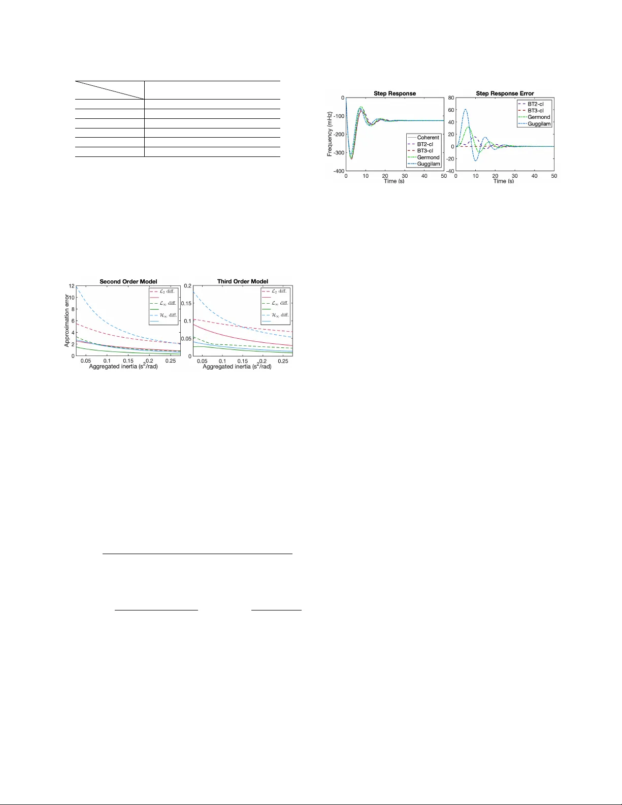
Loading high-quality paper...
Comments & Academic Discussion
Loading comments...
Leave a Comment