Algebraic Analysis of Rotation Data

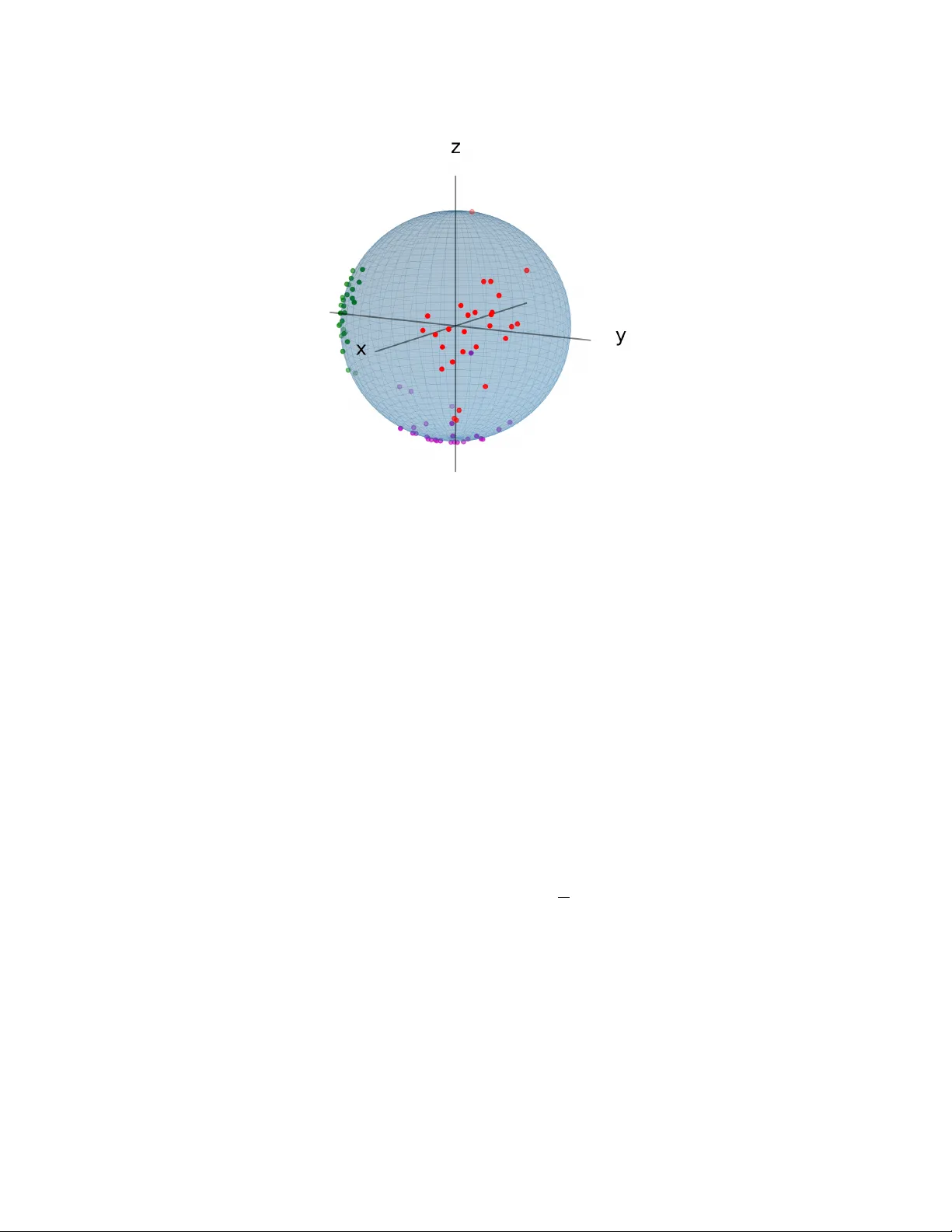
Algebraic Analysis of Rotation Data Mic hael F. Adamer, Andr´ as C. L˝ orincz, Anna-Laura Sattelb erger, and Bernd Sturmfels Abstract W e dev elop algebraic to ols for statistical inference from samples of rotation matrices. This rests on the theory of D -mo dules in algebraic analysis. Noncommutativ e Gr¨ obner bases are used to design n umerical algorithms for maximum lik elihoo d estimation, building on the holonomic gradien t method of Sei, Shibata, T akem ura, Ohara, and T ak a y ama. W e study the Fisher mo del for sampling from rotation matrices, and we apply our algorithms for data from the applied sciences. On the theoretical side, we generalize the underlying equiv arian t D -mo dules from SO(3) to arbitrary Lie groups. F or compact groups, our D -ideals encode the normalizing constan t of the Fisher mo del. 1 In tro duction Man y of the multiv ariate functions that arise in statistical inference are holonomic. Being holonomic roughly means that the function is annihilated b y a system of linear partial differen tial op erators with p olynomial co efficien ts whose solution space is finite-dimensional. Suc h a system of PDEs can b e written as a left ideal in the W eyl algebra, or D -ideal, for short. This representation allows for the application of algebraic geometry and algebraic analysis, including the use of computational tools, such as Gr¨ obner bases in the W eyl algebra [27, 29]. This imp ortan t connection betw een statistics and algebraic analysis w as first observ ed b y a group of sc holars in Japan, and it led to their dev elopmen t of the Holonomic Gr adient Metho d (HGM) and the Holonomic Gr adient Desc ent (HGD). W e refer to [10, 16, 30] and to further references given therein. The p oin t of departure for the present article is the work of Sei et al. [28], who developed HGD for data sampled from the rotation group SO( n ), and the article of Koy ama [16] who underto ok a study of the asso ciated equiv ariant D -mo dule. The statistical mo del w e examine in this article is the Fisher distribution on the group of rotations, defined in (1) and (2). The aim of maxim um lik eliho o d estimation (MLE) is to learn the model parameters Θ that b est explain a given data set. In our case, the MLE problem is difficult b ecause there is no simple form ula for ev aluating the normalizing constant of the distribution. This is where algebraic analysis comes in. The normalizing constant is a holonomic function of the mo del parameters, and we can use its holonomic D -ideal to deriv e an efficien t numerical scheme for solving the maximum likelihoo d estimation problem. The presen t pap er is organized as follo ws. Section 2 is purely exp ository . Here, we intro- duce the Fisher model, and we express its log-lik eliho o d function in terms of the sufficient 1 statistics of the giv en data. These are obtained from the singular v alue decomp osition of the sample mean. In Section 3, we turn to algebraic analysis. W e review the holonomic D -ideal in [28] that annihilates the normalizing constant of the Fisher distribution, and we derive its asso ciated Pfaffian system. P assing to n ≥ 3, w e next study the D -ideals on SO( n ) given in [16]. First new results can b e found in Theorem 3.4 and in Prop ositions 3.5 and 3.6. Section 4 is concerned with numerical algorithms for maximum lik eliho o d estimation. W e dev elop and compare Holonomic Gradient Ascent (HGA), Holonomic BF GS (H-BFGS) and a Holonomic Newton method. W e implemen ted these methods in the language R . Sec- tion 5 highligh ts ho w samples of rotation matrices arise in the sciences and engineering. T opics range from materials science and geology to astronomy and biomec hanics. W e apply holonomic metho ds to data from the literature, and w e discuss b oth successes and c hallenges. The D -ideal of the normalizing constan t is of independent in terest from the p ersp ective of represen tation theory , as it generalizes naturally to other Lie groups. The dev elopmen t of that theory is our main new mathematical con tribution. This w ork is presented in Section 6. 2 The Fisher mo del for random rotations In this section, we introduce the Fisher mo del on the rotation group, building on [28]. The group SO(3) consists of all real 3 × 3 matrices Y that satisfy Y t Y = Id 3 and det( Y ) = 1. This is a smo oth algebraic v ariety of dimension 3 in the 9-dimensional space R 3 × 3 . See [5] for a study of rotation groups from the p ersp ective of combinatorics and algebraic geometry . The Haar measure on SO(3) is the unique probability measure µ that is in v ariant under the group action. The Fisher mo del is a family of probabilit y distributions on SO(3) that is parametrized by 3 × 3 matrices Θ. F or a fixed Θ, the densit y of the Fisher distribution equals f Θ ( Y ) = 1 c (Θ) · exp(tr  Θ t · Y  ) for all Y ∈ SO(3) . (1) This is the density with resp ect to Haar measure µ . The denominator is the normalizing c onstant . It is chosen such that R SO(3) f Θ ( Y ) µ ( d Y ) = 1. This requiremen t is equiv alent to c (Θ) = Z SO(3) exp(tr(Θ t · Y )) µ ( d Y ) . (2) This function is the F ourier–Laplace transform of the Haar measure µ ; see Remark 6.6. The Fisher mo del is an exponential family . It is one of the simplest statistical mo dels on SO(3). The task at hand is the accurate numerical ev aluation of the in tegral (2) for given Θ in R 3 × 3 . W e b egin with the observ ation that, since in tegration is against the Haar measure, the function (2) is inv ariant under multiplying Θ on the left or right by a rotation matrix: c ( Q · Θ · R ) = c (Θ) for all Q, R ∈ SO(3) . In order to ev aluate (2), w e can therefore restrict to the case of diagonal matrices. Namely , giv en an y 3 × 3 matrix Θ, we first compute its sign-pr eserving singular value de c omp osition Θ = Q · diag( x 1 , x 2 , x 3 ) · R. 2 Figure 1: A dataset of 28 rotations from a study in v ectorcardiography [7], a metho d in medical imaging. Eac h p oin t represents the rotation of the unit standard vector on the x -axis (depicted in red color), the y -axis (green), and the z -axis (purple). This sample from the group SO(3) will b e analyzed in Section 5.1. Sign-preserving means that Q, R ∈ SO(3) and | x 1 | ≥ x 2 ≥ x 3 ≥ 0. F or non-singular Θ this implies that x 1 > 0 whenev er det(Θ) > 0 and x 1 < 0 otherwise. The normalizing constan t c (Θ) is the following function of the three singular v alues: ˜ c ( x 1 , x 2 , x 3 ) : = c (diag( x 1 , x 2 , x 3 )) = Z SO(3) exp( x 1 y 11 + x 2 y 22 + x 3 y 33 ) µ ( d Y ) . (3) The statistical problem w e address in this pap er is parameter estimation for the Fisher mo del. Supp ose we are giv en a finite sample { Y 1 , Y 2 , . . . , Y N } from the rotation group SO(3). W e refer to Figure 1 for a concrete example. Our aim is to find the parameter matrix Θ whose Fisher distribution f Θ b est explains the data. W e w ork in the classical framework of lik eliho o d inference, i.e., we seek to compute the maximum likelihoo d estimate (MLE) for the given data { Y 1 , Y 2 , . . . , Y N } . By definition, the MLE is the 3 × 3 parameter matrix ˆ Θ whic h maximizes the log-likelihoo d function. Th us, we m ust solv e an optimization problem. F rom our data w e obtain the sample me an ¯ Y = 1 N P N k =1 Y k . Of course, the sample mean ¯ Y is generally not a rotation matrix anymore. W e next compute the sign-preserving singular v alue decomp osition of the sample mean, i.e., w e determine Q, R ∈ SO(3) suc h that ¯ Y = Q · diag( g 1 , g 2 , g 2 ) · R. The signed singular v alues g 1 , g 2 , g 3 together with Q and R are sufficien t statistics for the Fisher mo del. The sample { Y 1 , . . . , Y N } enters the log-lik eliho o d function only via g 1 , g 2 , g 3 . Lemma 2.1. [28, Lemma 2] The lo g-likeliho o d function for the given sample fr om SO(3) is  : R 3 − → R , x 7→ x 1 g 1 + x 2 g 2 + x 3 g 3 − log( ˜ c ( x 1 , x 2 , x 3 )) . (4) 3 If ( ˆ x 1 , ˆ x 2 , ˆ x 3 ) is the maximizer of the function  , then the matrix ˆ Θ = Q diag ( ˆ x 1 , ˆ x 2 , ˆ x 3 ) R is the MLE of the Fisher mo del (1) of the sample { Y 1 , . . . , Y N } fr om the r otation gr oup SO(3) . Lemma 2.1 says that we need to maximize the function (4) in order to compute the MLE in the Fisher mo del. W e note that a lo cal maxim um is already a global one since (4) is a strictly concav e function. The maxim um is attained at a unique p oin t in R 3 . W e shall compute this p oint using to ols from algebraic analysis that are discussed in the next section. Remark 2.2. The singular v alues of the sample mean ¯ Y are bounded from abov e and below, namely 1 ≥ | g 1 | ≥ g 2 ≥ g 3 ≥ 0. If g 3 is close to 1, i.e., the a verage of the rotation matrices is almost a rotation matrix, then the data is typically concentrated ab out a preferred rotation. In this case the normalizing constant b ecomes very large and MLE on SO(3) is n umerically in tractable; see also Remark 4.3. Ho wev er, due to the small spread of the data around a p oin t in SO(3), a matrix v alued Gaussian mo del on R 3 is an accurate approximation. 3 Holonomic represen tation W e shall represen t the normalizing constan t ˜ c by a system of linear differential equations it satisfies. This is kno wn as the holonomic representation of this function. W e w ork in the Weyl algebr a D and in the r ational Weyl algebr a R with complex co efficients: D = C [ x 1 , x 2 , x 3 ] h ∂ 1 , ∂ 2 , ∂ 3 i and R = C ( x 1 , x 2 , x 3 ) h ∂ 1 , ∂ 2 , ∂ 3 i . W e refer to [27, 29] for basics on these tw o noncommutativ e algebras of linear partial dif- feren tial op erators with p olynomial and rational function co efficients, resp ectiv ely . In order to stress the n um b er of v ariables, w e sometimes write D 3 instead of D and R 3 instead of R . By a D -ide al we mean a left ideal in D , and b y an R -ide al a left ideal in R . The use of these algebras in statistical inference w as pioneered b y T akem ura, T ak a yama, and their collab orators [10, 16, 17, 28, 30]. W e b egin with an exp osition of their results from [28]. The normalizing constan t ˜ c is closely related to the hypergeometric function 0 F 1 of a matrix argumen t. In [28], annihilating differential op erators of ˜ c are deriv ed from H i = ∂ 2 i − 1 + X j 6 = i 1 x 2 i − x 2 j ( x i ∂ i − x j ∂ j ) for i = 1 , 2 , 3 . (5) These in turn can b e obtained from Muirhead’s differential op erators in [21, Theorem 7.5.6] b y a change of v ariables. In the notation of [27], w e hav e H i • ˜ c = 0 for i = 1 , 2 , 3. W ritten in the more familiar form of linear PDEs, this says ∂ 2 ˜ c ∂ x 2 i + X j 6 = i 1 x 2 i − x 2 j  x i ∂ ˜ c ∂ x i − x j ∂ ˜ c ∂ x j  = ˜ c for i = 1 , 2 , 3 . Note that the op erators H i are elements in the rational W eyl algebra R . Clearing the denominators, w e obtain elements G i in the W eyl algebra D that annihilate ˜ c , namely G i = Y j 6 = i ( x 2 i − x 2 j ) · H i . (6) 4 By [28, Theorem 1], the following three additional differential op erators in D annihilate ˜ c : L ij : = ( x 2 i − x 2 j ) ∂ i ∂ j − ( x i ∂ i − x j ∂ j ) − ( x 2 i − x 2 j ) ∂ k . (7) Here the indices are chosen to satisfy 1 ≤ i < j ≤ 3 and { i, j, k } = { 1 , 2 , 3 } . Let us consider the D -ideal that is generated by the six op erators in (6) and (7): I : = h G 1 , G 2 , G 3 , L 12 , L 13 , L 23 i . (8) In the rational W eyl algebra, w e hav e R I = h H 1 , H 2 , H 3 , L 12 , L 13 , L 23 i as R -ideals. W e en ter the D -ideal I in to the computer algebra system Singular:Plural as follo ws: ring r = 0,(x1,x2,x3,d1,d2,d3),dp; def D = Weyl(r); setring D; poly L12 = (x1^2-x2^2)*d1*d2 - (x2*d1-x1*d2)-(x1^2-x2^2)*d3; poly L13 = (x1^2-x3^2)*d1*d3 - (x3*d1-x1*d3)-(x1^2-x3^2)*d2; poly L23 = (x2^2-x3^2)*d2*d3 - (x3*d2-x2*d3)-(x2^2-x3^2)*d1; poly G1 = (x1^2-x2^2)*(x1^2-x3^2)*d1^2 + (x1^2-x3^2)*(x1*d1-x2*d2) + (x1^2-x2^2)*(x1*d1-x3*d3) - (x1^2-x2^2)*(x1^2-x3^2); poly G2 = (x2^2-x1^2)*(x2^2-x3^2)*d2^2 + (x2^2-x3^2)*(x2*d2-x1*d1) + (x2^2-x1^2)*(x2*d2-x3*d3) - (x2^2-x1^2)*(x2^2-x3^2); poly G3 = (x3^2-x1^2)*(x3^2-x2^2)*d3^2 + (x3^2-x2^2)*(x3*d3-x1*d1) + (x3^2-x1^2)*(x3*d3-x2*d2) - (x3^2-x1^2)*(x3^2-x2^2); ideal I = L12,L13,L23,G1,G2,G3; W e can no w perform v arious sym b olic computations in the W eyl algebra D . W e used the libraries dmodloc [1] and dmod [18], due to Andres, Lev andovskyy , and Mart ´ ın-Morales. In particular, the follo wing tw o lines confirm that I is holonomic and its holonomic rank is 4: isHolonomic(I); holonomicRank(I); The rank statemen t means algebraically that dim C ( x 1 ,x 2 ,x 3 ) ( R/RI ) = 4. In terms of analysis, it means that the set of holomorphic solutions to I on a small op en ball U ⊂ C 3 is a 4-dimensional vector space. Here U is chosen to b e disjoint from the singular lo cus Sing( I ) =  x ∈ C 3 : ( x 2 1 − x 2 2 )( x 2 1 − x 2 3 )( x 2 2 − x 2 3 ) = 0  . (9) W e note that the normalizing constant ˜ c = ˜ c ( x 1 , x 2 , x 3 ) is a real analytic function on R 3 \ Sing( I ) that extends to a holomorphic function on all of complex affine space C 3 . Using Gr¨ obner bases in the rational W eyl algebra R , w e find that the initial ideal of RI for the degree reverse lexicographic order is generated by the sym b ols of our six operators: in( RI ) = h ∂ 1 ∂ 2 , ∂ 1 ∂ 3 , ∂ 2 ∂ 3 , ∂ 2 1 , ∂ 2 2 , ∂ 2 3 i . The set of standard monomials equals S = { 1 , ∂ 1 , ∂ 2 , ∂ 3 } . This is a C ( x 1 , x 2 , x 3 )-basis for the vector space R/R I . In this situation, w e can associate a Pfaffian system to the D -ideal I . F or the general theory , we refer the reader to [29] and sp ecifically to [27, Equation (23)]. The Pfaffian system is a system of first-order linear differen tial equations asso ciated to the holonomic function ˜ c . It consists of three 4 × 4 matrices P 1 , P 2 , P 3 whose entries are rational functions in x 1 , x 2 , x 3 . W e introduce the column v ector C = ( ˜ c, ∂ 1 • ˜ c, ∂ 2 • ˜ c, ∂ 3 • ˜ c ) t . 5 Theorem 3.1. [28, Theorem 2] The Pfaffian system asso ciate d to the normalizing c on- stant ˜ c of the Fisher distribution (1) c onsists of the fol lowing thr e e ve ctor e quations: ∂ i • C = P i · C for i = 1 , 2 , 3 , (10) wher e the matric es P 1 , P 2 , P 3 ∈ C ( x 1 , x 2 , x 3 ) 4 × 4 ar e P 1 =      0 1 0 0 1 x 1 ( − 2 x 2 1 + x 2 2 + x 2 3 ) ( x 2 1 − x 2 3 )( x 2 1 − x 2 2 ) x 2 x 2 1 − x 2 2 x 3 x 2 1 − x 2 3 0 x 2 x 2 1 − x 2 2 − x 1 x 2 1 − x 2 2 1 0 x 3 x 2 1 − x 2 3 1 − x 1 x 2 1 − x 2 3      , P 2 =      0 0 1 0 0 − x 2 x 2 2 − x 2 1 x 1 x 2 2 − x 2 1 1 1 x 1 x 2 2 − x 2 1 x 2 ( x 2 1 − 2 x 2 2 + x 2 3 ) ( x 2 2 − x 2 1 )( x 2 2 − x 2 3 ) x 3 x 2 2 − x 2 3 0 1 x 3 x 2 2 − x 2 3 − x 2 x 2 2 − x 2 3      , and P 3 =      0 0 0 1 0 − x 3 x 2 3 − x 2 1 1 x 1 x 2 3 − x 2 1 0 1 − x 3 x 2 3 − x 2 2 x 2 x 2 3 − x 2 2 1 x 1 x 2 3 − x 2 1 x 2 x 2 3 − x 2 2 x 3 ( x 2 1 + x 2 2 − 2 x 2 3 ) ( x 2 3 − x 2 1 )( x 2 3 − x 2 2 )      . W e repro duced this Pfaffian system from the op erators G 1 , G 2 , G 3 , L 12 , L 13 , L 23 with the Mathematica pac k age HolonomicFunctions [15]. This w as done by running Gr¨ obner basis computations in the rational W eyl algebra R with the degree rev erse lexicographic order. See [27, Example 3.4] for an illustration on how this is done. The Pfaffian system (10) allows us to reco v er the i th partial deriv ative of the normalizing constan t as the first co ordinate of the column v ector P i · C . In sym b ols w e hav e ∂ i • ˜ c = ( P i · C ) 1 . W e mak e extensiv e use of this fact when computing the MLE in Section 4. In the same v ein, we can recov er the Hessian of ˜ c from the Pfaffian system of ˜ c as follows: ∂ 2 1 • ˜ c = ( P 1 · C ) 2 , ∂ 1 ∂ 2 • ˜ c = ( P 2 · C ) 2 , ∂ 1 ∂ 3 • ˜ c = ( P 3 · C ) 2 , ∂ 2 2 • ˜ c = ( P 2 · C ) 3 , ∂ 2 ∂ 3 • ˜ c = ( P 3 · C ) 3 , ∂ 2 3 • ˜ c = ( P 3 · C ) 4 . (11) This allo ws for the use of second order optimization algorithms, see Section 4. An ob ject of in terest—from the algebraic analysis p ersp ective—is the W eyl closure of the D -ideal I . By definition, the Weyl closur e is the follo wing D -ideal which clearly contains I : W ( I ) : = RI ∩ D . In general, it is a challenging problem to compute the W eyl closure of a D -ideal. This computation is reminiscent of finding the radical of a p olynomial ideal, which, according to Hilb ert’s Nullstellensatz, consists of all p olynomials that v anish on the complex solutions to the given p olynomials. The W eyl closure plays a similar role for holonomic functions. It turns out that computing W ( I ) is fairly b enign for the D -ideal I studied in this section. Lemma 3.2. Let I be the holonomic D -ideal in (8). Then the W eyl closure W ( I ) is generated by I and the one additional op erator x 1 ∂ 1 ∂ 3 + x 2 ∂ 2 ∂ 3 + x 3 ∂ 2 3 − x 2 ∂ 1 − x 1 ∂ 2 − x 3 + 2 ∂ 3 . Pr o of. W e used the Singular library dmodloc [1] to compute the W eyl closure of I . W e found that I is not W eyl-closed, i.e., I ( W ( I ). Moreo v er, by Gr¨ obner basis reductions in the W eyl algebra, w e find that adding the claimed operator results in a W eyl-closed ideal. 6 F ollowing [16, 28], w e no w consider the Fisher distribution on SO( n ). The normalizing constan t c (Θ) is defined as in (2), with the integral taken ov er SO( n ) with its Haar measure. Let D n 2 b e the W eyl algebra whose v ariables are the entries of the n × n matrix Θ = ( t ij ). The corresponding n × n matrix of differen tial op erators in D n 2 is denoted by ∂ = ( ∂ ij ). The follo wing result w as established by Koy ama [16], based on earlier work of Sei et al. [28]. W e shall prov e a more general statement for arbitrary compact Lie groups in Section 6. Theorem 3.3. The annihilator of c (Θ) is the D -ideal generated by the follo wing op erators: d = 1 − det( ∂ ) , g ij = δ ij − P n k =1 ∂ ik ∂ j k for 1 ≤ i ≤ j ≤ n, P ij = P n k =1  t ik ∂ j k − t j k ∂ ik  for 1 ≤ i < j ≤ n. Ab o v e w e omitted half of the equations given in [16, Equation (12)], whic h is justified b y the results in [24, Section 8.7.3]. Also, the op erators P ij are induced from left matrix m ultiplication (as in (26)) rather than right multiplication as in [16, Equation (11)]. A problem that was left op en in [16, 28], even for n = 3, is the determination of the holonomic rank of J . W e now address this b y introducing dimensionality reduction via in v arian t theory . Let J 0 b e the D -ideal generated b y the op erators P ij , g ij . This is the analogue of J for the orthogonal group O( n ) in its standard represen tation in GL n ( C ) (see Section 6). Since O( n ) has t wo connected comp onen ts, the corresp onding mo dule in Theorem 6.2 is a direct sum of t w o simple holonomic D n 2 -mo dules. By symmetry , w e obtain rank( J 0 ) = 2 · rank( J ) . (12) The ring of O( n )-in v arian t p olynomials on C n × n is generated by the  n +1 2  en tries { y kl } 1 ≤ k ≤ l ≤ n of the symmetric matrix Y = Θ t · Θ (see [24, Section 11.2.1]). These ma- trix en tries y kl are algebraically indep enden t quadratic forms in the n 2 unkno wns t ij . W e no w work in the W eyl algebra D ( n +1 2 ) with the con ven tion y kl = y lk and ∂ kl = ∂ lk . Let K denote the left ideal in that W eyl algebra which is generated by the operators h ij = 2 δ ij n · ∂ ij − δ ij + n X k, l =1 2 δ ki + δ lj y kl · ∂ ik ∂ j l for 1 ≤ i ≤ j ≤ n. (13) Theorem 3.4. A holomorphic function is a solution to J 0 if and only if it is of the form Θ 7→ φ ( y ij (Θ)), where φ is a solution to K . In particular, rank( K ) = 2 · rank( J ). Pr o of. The Lie algebra op erators P ij express left in v ariance under SO( n ). The fact that ev ery solution to J 0 is expressible in Y follo ws from Luna’s Theorem [19] (see also [11, Section 6.4]). W e note that the determinan t det(Θ) is an SO( n )-inv ariant that w e ma y omit, due to the relation det(Θ) 2 = det Y . The D -ideal K is the inv arian t v ersion of J 0 . The op erator h ij is deriv ed from g ij b y the c hain rule. The result therefore follo ws from (12). As an application of Theorem 3.4, we answer a question left op en in [28, Prop osition 2]. Prop osition 3.5. F or n = 3, we hav e rank( J ) = 4. 7 Pr o of. W e used the computer algebra system Macaulay2 [9]. Unlik e for rank( J ), the calcu- lations for rank( K ) finished, and w e found rank( K ) = 8. W e conclude by Theorem 3.4. W e next explain how the D n 2 -ideal J and the D n -ideal I in (8) are connected. The ideal I is defined as in (8) for all n . W e use the construction of the r estriction ide al . F or the general definition see [27, Equation (13)]. In our case, the construction works as follows. W e set x i = t ii for i = 1 , . . . , n and w e write D n for the corresp onding W eyl algebra. Then J diag : =  J +  t ij : 1 ≤ i 6 = j ≤ n  · D n 2  ∩ D n (14) is the D n -ideal obtained b y restricting the annihilator of c (Θ) to the diagonal en tries of the matrix Θ. Note that the second summand in (14) is a right ideal in the W eyl algebra D n 2 . If f (Θ) is a function in the n 2 v ariables t ij that is annihilated b y J , then the restriction ideal J diag annihilates the function f (diag( x 1 , . . . , x n )) in n v ariables. Therefore, J diag annihilates the restricted normalizing constant ˜ c ( x 1 , . . . , x n ). W e hav e the following result. Prop osition 3.6. The following inclusions hold among holonomic D n -ideals represen ting ˜ c : I ⊆ J diag ( W ( J diag ) ⊆ ann D n (˜ c ) . Equalit y holds for n ≤ 3 in the rightmost inclusion. Pr o of sketch. The pro of of [28, Theorem 1] sho ws that I is con tained in J diag . The middle inclusion is strict b y Lemma 3.2. W e hav e W ( J diag ) ⊆ ann D n (˜ c ) b ecause the annihilator of a smo oth function suc h as ˜ c is W eyl-closed, by an argument sp elled out in [8]. The equality on the right for n = 3 is shown b y proving W ( I ) = ann D 3 (˜ c ). W e use the follo wing argumen t and computations. The F ourier transform W ( I ) F is the D -ideal obtained b y switching ∂ i and x i (up to sign). W e find that its holonomic rank is 1. W e next compute the holonomic dual of the mo dule D 3 /W ( I ) F . This is another D 3 -mo dule, as defined in [12, Section 2.6]. There is a built-in command for the holonomic dual in Macaulay2 [9]. Another computation, using lo calization techniques, verifies that b oth D 3 /W ( I ) F and its holonomic dual are torsion-free as C [ x 1 , x 2 , x 3 ]-mo dules. These facts imply that D 3 /W ( I ) F is a simple D -mo dule, and hence so is D 3 /W ( I ). F rom this w e conclude that W ( I ) = ann D 3 (˜ c ). W e conjecture that the inclusion on the right is an equality for all p ositive integers n . Using results from Section 6, w e can argue that W ( J diag ) F is regular holonomic for any n . It app ears that its singular lo cus is a hyperplane arrangement. The sp ecial com binatorial structure encoun tered in this arrangement gives strong evidence for the conjecture ab ov e. 4 Maxim um lik eliho o d estimation W e no w pro ceed to finding the maxim um of the log-likelihoo d function of Lemma 2.1 for giv en datasets. Since the ob jectiv e function (4) is strictly concav e, a local maxim um is the global maximizer and attained at a unique p oint ˆ x = ( ˆ x 1 , ˆ x 2 , ˆ x 3 ) ∈ R 3 . In order to compute ˆ x , w e run a num b er of algorithms, each using the holonomic gradient metho d. This is based on 8 the results presented in the previous section, esp ecially on Theorem 3.1 and Equation (11). These are used to compute the function v alues, gradients, and Hessians in each iteration. A critical step in running any lo cal optimization metho d is finding a suitable starting p oin t. As men tioned in Section 3, solutions to the D -ideal I are analytic outside the singular lo cus Sing( I ). Starting points need to b e c hosen in R 3 \ Sing( I ). F or the Fisher mo del on SO(3), the singular lo cus Sing( I ) is the arrangemen t (9) of six planes through the origin in R 3 . This partitions R 3 in to 24 distinct c hambers. F or the algorithms describ ed b elow, we c ho ose starting p oin ts in each of the 24 connected comp onents of R 3 / Sing( I ), and we ev aluate the v ector C at these p oin ts. This initialization can b e done either via the series expansion metho d of [28, Section 3.2] or using the pack age hgm [30] in the statistical softw are R . In this section, we present three optimization methods based on algebraic analysis. The simplest is Holonomic Gr adient Asc ent (HGA). This is a straightforw ard adaptation of the HGD metho d in [28]. Second, w e introduce a holonomic version of the Broyden–Fletc her– Goldfarb–Shanno (BF GS) metho d [22, Chapter 6, § 1]. BFGS is a quasi-Newton metho d that requires the gradien t and the function v alue as inputs. Both can b e calculated directly using (10). This turns BF GS into Holonomic BF GS (H-BF GS). The third algorithm to b e in tro duced is a Holonomic Newton Metho d . This second-order metho d exploits the fact that the Hessian is easy to calculate from (11) and that the ob jectiv e function is strictly conca v e. T o get started, w e need an expression for the gradient of the log-likelihoo d function  and a Holonomic Gradient Metho d (HGM) for ev aluating that expression. By Lemma 2.1, ∇  ( x ) =   g 1 g 2 g 3   − 1 ˜ c ( x ) · ∇ ˜ c ( x ) . (15) Note that C ( x ) = ( ˜ c ( x ) , ∇ ˜ c ( x )) t . Hence, our task to ev aluate ∇  at any p oin t amounts to ev aluating the v ector-v alued function C at any p oint. This is where the HGM comes in. In general, w e appro ximate the function C at a point x ( n +1) giv en its v alue at a previous p oin t x ( n ) . T o this end, a path x ( n ) → x ( n ) + δ (1) → x ( n ) + δ (2) → · · · → x ( n ) + δ ( K ) → x ( n +1) is chosen, where δ (1) , . . . , δ ( K ) ∈ R 3 with k δ ( m +1) − δ ( m ) k sufficiently small. The linear part of the T a ylor series expansion of C at x ( n ) yields the follo wing approximations: C ( x ( n ) + δ ( m +1) ) ≈ C ( x ( n ) + δ ( m ) ) + 3 X i =1 ( δ ( m +1) i − δ ( m ) i ) ( ∂ i • C )( x ( n ) + δ ( m ) ) = C ( x ( n ) + δ ( m ) ) + 3 X i =1 ( δ ( m +1) i − δ ( m ) i ) P i · C ( x ( n ) + δ ( m ) ) . (16) W e choose a path consisting of p oints, separated by interv als of size ∆ t , on the line segmen t x ( t ) = x ( n ) (1 − t ) + x ( n +1) t with t ∈ [0 , 1]. With this notation, Equation (16) b ecomes C ( x (( m + 1)∆ t )) ≈ C ( x ( m ∆ t )) + P 3 i =1 ( x ( n +1) i − x ( n ) i ) ∆ t · P i · C ( x ( m ∆ t )) . (17) If w e take the limit ∆ t → 0, then the equation ab o ve b ecomes the differential equation dC ( t ) dt = 3 X i =1 ∂ x i ∂ t ∂ C ∂ x i = 3 X i =1  x ( n +1) i − x ( n ) i  P i · C. 9 This ordinary differen tial equation can b e solved using an y n umerical ODE solver, e.g., an Euler sc heme or Runge–Kutta scheme. This leads to the following algorithm. Algorithm 1: Holonomic Gradien t Metho d Input: x ( n ) , x ( n +1) , C ( x ( n ) ), a Pfaffian system P 1 , P 2 , P 3 Output: C ( x ( n +1) ) 1 Set x ( t ) = x ( n ) (1 − t ) + x ( n +1) t . 2 Let dC ( t ) dt = P 3 i =1 ∂ x i ∂ t ∂ C ∂ x i = P 3 i =1  x ( n +1) i − x ( n ) i  P i · C . 3 Numerically integrate line 2 from t = 0 to t = 1. W e emplo y Algorithm 1 as a subroutine for the holonomic gradient ascent algorithm, whic h will be describ ed next. HGA is analogous to other gradient ascen t/descent metho ds, ho w ever, with the sp ecial feature that the gradients are calculated via the HGM algorithm. A description of the algorithm, adapted for data from SO(3), is outlined b elow. Algorithm 2: Holonomic Gradien t Ascent Input: Matrices Q and R , singular v alues g 1 , g 2 , g 3 and a starting p oin t x (0) ∈ R 3 Result: A maximum likelihoo d estimate for the data in the Fisher mo del (1) 1 Cho ose a learning rate γ n . 2 Cho ose a threshold δ . 3 Ev aluate C at the starting point x (0) . 4 Ev aluate ∇  at the starting p oint x (0) . 5 Set n = 0. 6 while max |∇  ( x ( n ) ) | < δ do 7 x ( n +1) = x ( n ) + γ n ∇  ( x ( n ) ). 8 Calculate C ( x ( n +1) ) via HGM using Algorithm 1. 9 Calculate ∇  ( x ( n +1) ) from C ( x ( n +1) ). 10 Set n = n + 1. 11 end 12 Output vector x ( n ) ∈ R 3 as our appro ximation for ( ˆ x 1 , ˆ x 2 , ˆ x 3 ). 13 Output the rotation matrix ˆ Θ = Q · x ( n ) · R as our appro ximation for the MLE. The giv en data is a list of rotation matrices Y 1 , . . . , Y N in SO(3). As explained in Sec- tion 2, w e enco de these in the singular v alues g 1 , g 2 , g 3 of the sample mean ¯ Y = 1 N P N k =1 Y k . Th us, the input for HGA consists primarily of just three num b ers g 1 , g 2 , g 3 . They are used in the ev aluation in the first terms of ∇  , as seen in (15). The second term is ev aluated b y matrix m ultiplication with P 1 , P 2 , P 3 , as seen in (10). P art of the input are also the matrices Q and R that diagonalize the sample mean ¯ Y . They are needed in the last step to re- co v er ˆ Θ from ˆ x 1 , ˆ x 2 , ˆ x 3 as in Lemma 2.1. The HGA algorithm has t w o parameters, namely the threshold δ whic h indicates a termination condition, and the learning rate γ n . While δ can be c hosen freely dep ending on the desired accuracy , choosing the learning rate can 10 ha v e significan t effects on the con vergence of the algorithm. In our computations w e c hose γ n = 10 − 2 . This can clearly b e impro ved. How ever, the standard tec hnique of p erforming line searc hes to find a go od γ n is not recommended as ev aluating C at a new p oin t is costly . T o employ more adv anced metho ds such as BF GS, and to av oid in tegrating along a path crossing the singular lo cus, w e use [28, Corollary 1]. This states that the v alue of C at a p oin t ( x 1 , x 2 , x 3 ) can b e obtained b y integrating the follo wing ODE from t =   1 to t = 1: dC dt =     0 x 1 x 2 x 3 x 1 − 2 /t x 3 x 2 x 2 x 3 − 2 /t x 1 x 3 x 2 x 1 − 2 /t     · C. (18) Using this approach for calculating C , we can emplo y BFGS optimization using HGM as a subroutine to calculate the gradients and function v alues required as inputs. The H-BF GS metho d achiev es m uch faster conv ergence rates than the simple HGA algorithm 2. A final v ery p ow erful algorithm for concav e (or conv ex) functions is the Newton metho d whic h uses the Hessian matrix. Often, finding the Hessian matrix H [  ( x )] of a function is a difficult task. How ever, using holonomic methods the Hessian is a obtained for free via ∂ i ∂ j •  = 1 ˜ c 2 ( ∂ i • ˜ c ) ( ∂ j • ˜ c ) − 1 ˜ c ∂ i ∂ j • ˜ c, and the relations in (10) and (11). W e found that the Newton metho d, x ( n +1) = x ( n ) − H [  ( x )] − 1 · ∇  ( x ) , giv es the fastest conv ergence. W e refer to this approach as the Holonomic Newton Metho d . W e implemen ted the H-BFGS metho d in a script in the soft w are R . Interested readers may obtain our implementation from the first author. This co de is custom-tailored for rotations in 3-space. The function C is ev aluated at the starting p oin t x (0) using the series expansion metho d that is describ ed in [28, Section 3.2]. Here we truncate the series at order 41. Example 4.1. W e created a syn thetic dataset consisting of N = 500 rotation matrices. These w ere sampled from the Fisher distribution with parameter matrix Θ =   − 1 . 178 0 . 2804 1 . 037 − 0 . 3825 0 . 9181 0 . 6016 − 0 . 0955 0 . 9037 1 . 695   . (19) The sample mean and its sign-preserving singular v alue decomp osition are found to b e ¯ Y =   − 0 . 2262 0 . 1021 0 . 2260 − 0 . 0233 0 . 0611 0 . 2779 − 0 . 0364 0 . 2802 0 . 3529   = Q ·   0 . 5946 0 . 0000 0 . 0000 0 . 0000 0 . 1838 0 . 0000 0 . 0000 0 . 0000 0 . 1059   · R, with Q =   − 0 . 4977 0 . 8589 0 . 1211 − 0 . 4518 − 0 . 1376 − 0 . 8815 − 0 . 7404 − 0 . 4934 0 . 4565   , R =   0 . 2524 − 0 . 4808 − 0 . 8397 − 0 . 9419 − 0 . 3209 − 0 . 0993 − 0 . 2217 0 . 8160 − 0 . 5339   . 11 Running H-BF GS on this input, the MLE is found to b e ˆ Θ =   − 0 . 8972 0 . 3446 0 . 9682 − 0 . 2392 0 . 7777 0 . 7856 − 0 . 0763 0 . 8664 1 . 616   = Q ·   2 . 422 0 . 0000 0 . 0000 0 . 0000 0 . 7432 0 . 0000 0 . 0000 0 . 0000 − 0 . 3043   · R. (20) While the en tries of the MLE ˆ Θ hav e the correct sign and order of magnitude, the actual v alues are not v ery close to those in Θ. In order to isolate the effect of the sample size on the MLE, w e extended the data to 10000 matrices. In the iterations we recorded the F rob enius distance (FD) from ˆ Θ to Θ and the logarithm of the likelihoo d ratio (LR) of the exact parameter and the MLE. Our findings are outlined in the table below. # Data H-BF GS FD Newton FD H-BFGS LR Newton LR 1000 0.2136 0.2136 0.07006 -0.0007 2000 0.1145 0.1145 0.08828 -0.0013 3000 0.1155 0.1155 0.07837 -0.0012 4000 0.1485 0.1485 0.08185 -0.0014 5000 0.1700 0.1700 0.07439 -0.0009 6000 0.1247 0.1247 0.07325 -0.0006 7000 0.1321 0.1321 0.07248 -0.0006 8000 0.1011 0.1011 0.07294 -0.0003 9000 0.0985 0.0985 0.07127 -0.0002 10000 0.0838 0.0838 0.07219 -0.0002 In our experiments we found that the con vergence in likelihoo d ratio and F rob enius distance is slow. It app ears that, in general, the MLE problem is not v ery w ell conditioned. Remark 4.2. The authors in [28] rep ort that the HGD algorithm b ecomes numerically un- stable when it is close to the singular lo cus of the Pfaffian system. They recommend pic king a starting p oin t in the same connected comp onen t of R 3 \ Sing( I ) where the MLE is suspected. In contrast, our computations suggest that the output of the HGA do es not depend on the connected comp onen t which the starting p oint lies in, when a sufficiently stable n umerical in tegration metho d (e.g. lsode from the R pack age deSolve ) is chosen in Algorithm 1. Remark 4.3. The sample mean matrix ¯ Y lies in the con v ex h ull of the rotation group. This conv ex b o dy , denoted con v (SO(3)), w as studied in [26, Section 4.4], and an explicit represen tation as a sp ectrahedron w as given in [26, Prop osition 4.1]. It follo ws from the theory of orbitop es [26] that the singular v alues of matrices in conv(SO(3)) are precisely the triples that satisfy 1 ≥ | g 1 | ≥ g 2 ≥ g 3 ≥ 0. These inequalities define tw o p olytop es, which are resp onsible for the facial description of con v(SO(3)) found in [26, Theorem 4.11]. W e can think of the MLE as a map from the interior of the orbitop e con v (SO(3)) to R 3 . Using the singular v alue decomp osition, we restricted this map to the op en p olytop es given b y 1 > | g 1 | > g 2 > g 3 > 0. Note that the co ordinates of the v ector ˆ x go es off to infinit y as the maxim um of { g 1 , g 2 , g 3 } approac hes 1. This follo ws from [14, Equation (4.12)], where the analogue for O( n ) was derived. This divergence can cause numerical problems. 12 In this section, we ha ve turned the earlier results on D -ideals in to n umerical algorithms. This is just a first step. The success of any lo cal metho d relies hea vily on a clear under- standing of the numerical analysis that is relev ant for the problem at hand. A future study of condition n umbers from the p ersp ectiv e of holonomic representations w ould b e desirable. 5 Rotation data in the sciences Rotation data arise in an y field of science in which the orientation of an ob ject in 3-space is imp ortan t. Occurrences include a diverse num b er of researc h areas such as medical imaging, biomec hanics, astronomy , geology , and materials science. In this section, we apply our metho ds to a prominen t dataset of v ectorcardiograms and to biomechanical data. W e also review previous findings on rotation data in astronom y , geology , and materials science. 5.1 Medical imaging One imp ortan t o ccurrence of rotational data in the applied sciences stems from medical imaging, and more precisely from v ectorcardiograph y . In that field, the electrical forces generated b y the heart are studied and their magnitude and direction are recorded. The dataset presen ted in [7] is a famous example of directional data. It contains the orien tation of the vectorcardiogram (VC) lo op of 98 c hildren aged 2 − 19. In particular, the orientation is measured using t w o differen t techniques. Both measuremen ts are given in the form of t w o vectors. The first identifies the VC loop of greatest magnitude and the second is the normal direction to the lo op. W e add as a third vector the cross pro duct of the magnitude and normal vector to form a right handed set and, therefore, a rotation matrix. This dataset has b een used to exemplify a range of metho ds in directional statistics, see, e.g., [23]. W e applied the optimization metho ds from Section 4 to the same dataset. In other w ords, w e computed the maxim um of the log-likelihoo d function (4) for the orientations of the V C lo op. In order to match our analysis with the results of [23], we only consider the 28 data p oin ts of the b o ys aged 2 − 10. A colorful illustration of the action of these 28 rotation matrices on the co ordinate axes is shown in Figure 1. W e no w pro ceed to the MLE. The sample mean has the singular v alued decomposition ¯ Y =   0 . 6868 0 . 5756 0 . 1828 0 . 5511 − 0 . 7372 − 0 . 0045 0 . 1216 0 . 1417 − 0 . 8630   = Q ·   0 . 9469 0 . 0000 0 . 0000 0 . 0000 0 . 8962 0 . 0000 0 . 0000 0 . 0000 0 . 8737   · R, (21) where Q =   0 . 6112 0 . 7636 0 . 2079 − 0 . 7498 0 . 4748 0 . 4608 0 . 2532 − 0 . 4376 0 . 8628   , R =   0 . 03941 0 . 99324 − 0 . 1092 0 . 81778 0 . 03072 0 . 5747 0 . 57418 − 0 . 11194 − 0 . 8110   . (22) By forming the matrix pro duct QR w e recov er the result of [23]. The matrix QR , how ever, is only one part of the MLE as describ ed in [14]. By using H-BF GS, w e can find the full MLE of the Fisher mo del. W e compared H-BFGS to other metho ds. F or that, we estimated 13 x 1 , x 2 , x 3 with a BFGS optimization of the log-likelihoo d using the series expansion of the normalizing constan t. W e then compare the resulting estimate to the output of H-BFGS. The H-BF GS algorithm finds the MLE ˆ x 1 = 20 . 072407 , ˆ x 2 = 12 . 513841 , ˆ x 3 = − 6 . 510704 , whic h corresponds to a log-lik eliho o d of ˆ  = 3 . 97299. The run time of the algorithm is highly dep enden t on the n um b er of non-zero terms in the series expansion for ˜ c . In this calculation, the first 6000 non-zero terms are used and the runtime is about 4 seconds. The classical BF GS method is not conv ergent if only the first 6000 non-zero terms are used. Hence, w e need to truncate the series expansion at higher order. If w e use the first 48000 non- zero terms, then the series expansion BF GS method finds the MLE ˆ x 1 = 17 . 604156 , ˆ x 2 = 10 . 024591 , ˆ x 3 = − 3 . 881811, which gives ˆ  = 3 . 96330. The computation takes ab out 20 seconds. Hence, the holonomic BFGS outp erformed the classical metho d b y finding a b etter lik eliho o d v alue in muc h shorter time. 5.2 Biomec hanics Rotational data is ubiquitous in the biomedical sciences. A prominent experiment in this area is the h uman kinematics study of [25]. In this exp erimen t, the rotations of four differen t upp er b o dy parts w ere track ed while the sub ject was drilling holes in to six different lo cations of a v ertical panel. In [4], this dataset was studied and maximum likelihoo d and Bay esian p oint estimates for the orientation of the wrist were obtained and credible regions constructed. A further exp eriment concerns the heel orientation of primates. In the exp eriments, the rotation of the calcaneus b one (the heel) and the cuboid b one, which is horizon tally adjacent to the heel and closer to the to es, w as measured. A load w as applied to three sedentary primates, a human, a c himpanzee, and a bab o on and the rotation of their ankle w as recorded. While the data is actually a time series, the simplifying assumption of indep enden t iden tically distributed data is made in its analysis [3]. W e study this dataset whic h w as kindly provided b y Melissa Bingham. The sample mean for the human data equals ¯ Y =   − 0 . 1013 − 0 . 9127 − 0 . 3811 0 . 3275 − 0 . 3895 0 . 8535 − 0 . 9335 − 0 . 0358 0 . 3475   = Q ·   0 . 9997 0 . 0000 0 . 0000 0 . 0000 0 . 9926 0 . 0000 0 . 0000 0 . 0000 0 . 9923   · R, (23) with Q =   0 . 4771 0 . 8753 − 0 . 0791 − 0 . 4320 0 . 1552 − 0 . 8884 − 0 . 7654 0 . 4580 0 . 4521   and R =   0 . 5248 − 0 . 2399 − 0 . 8167 − 0 . 4690 − 0 . 8822 − 0 . 0422 − 0 . 7104 0 . 4051 − 0 . 5754   . W e see on the right hand side in (23) that the singular v alues for this dataset only differ in the third significant figure and the smallest singular v alue is approximately 1. W e found that the normalizing constan t gets to o large to b e computed directly . Indeed, our simulations returned a v alue error when ˜ c ≈ 10 308 . This is a serious numerical issue, arising in an y MLE 14 algorithm that attempts to directly calculate ˜ c when the sample mean is almost a rotation matrix. Singular v alues close to one imply that the samples are concentrated on the unit sphere. One could either use a rotational Maxw ell distribution [13] as a lo cal model or the appro ximation used in [3]. The data for the bab o on and the c himpanzee sho w similar traits. W e found that progress can be made b y applying a gauge transform in Equation (18), aimed at scaling the input for H-BFGS. Let λ 0 b e the largest eigenv alue of A =     0 x 1 x 2 x 3 x 1 0 x 3 x 2 x 2 x 3 0 x 1 x 3 x 2 x 1 0     . W e can deriv e an ODE for the function D = C · exp( − λ 0 t ) from Equation (18). The function D is guaran teed to ha ve smaller v alues than C . F urthermore, the ratio ( ∂ i • ˜ c ) / ˜ c = C i /C 0 = D i /D 0 is in v ariant. Despite b eing able to compute log (˜ c ) using the gauge transformation, MLE b ecomes v ery unstable due to the n umerical accuracy required. Finding the MLE from a random starting p oin t using H-BF GS prov ed in tractable. Ho wev er, using the asymptotic form ula of [14] to provide a suitable starting p oint for H-BF GS, we found the MLE ˆ x 1 = 5543 . 106 , ˆ x 2 = 3753 . 078 , ˆ x 3 = − 3685 . 242 corresp onding to a log-likelihoo d of ˆ  = 10 . 59342. The asymptotic form ula yielded an MLE of ˆ x 1 = 5543 . 102 , ˆ x 2 = 3753 . 025 , ˆ x 3 = − 3685 . 298 and ˆ  = 10 . 52366. Hence, H-BFGS finds a sligh tly b etter MLE than the asymptotic form ula. 5.3 Astronom y and geology Astronomical applications of the matrix Fisher mo del on SO(3) are often concerned with the orbits of near earth ob jects [20, 28]. Suc h ob jects are comets or asteroids in an elliptic orbit around the sun with the sun in their fo cus. The data comes as sets of vectors in R 3 taking the sun as the origin. The first v ector, X 1 , is the p erihelion direction, which points to the lo cation on the orbit closest to the sun. The second vector, X 2 , is the unit normal to the orbit. T ogether with their cross pro duct these v ectors form a right handed set. Therefore, they define a rotation matrix. Questions of astronomical interest are whether the p erihelion direction is uniformly distributed on the sphere and whether the orbit orien tations are uniform on SO(3). T o answer the latter question the Raleigh statistic can b e used [20, 28]. Sei et al. [28] studied a dataset of rotations representing 151 comets and 6496 asteroids. They computed maximum likelihoo d estimates using the holonomic gradien t metho d and also series expansions. The Raleigh statistic for the dataset w as calculated and the n ull h yp othesis of a uniform distribution was strongly rejected. F urther, the h yp othesis of the data originating from a Fisher distribution on a Stiefel manifold w as tested against the h yp othesis of SO(3), and the evidence strongly suggested to reject the Stiefel manifold. Rotations arise in geology and earth sciences in the study of earthquake epicen ters [13] and the analysis of plate tectonics [6]. Davis and Titus [6] studied a dataset of the deformation of a shear zone in northern Idaho. Ho wev er, this was done in the context of inv alidating a geology inspired mo del that had b een used previously to explain the shear deformations. Kagan [13] studied rotational data describing the earthquak e fo cal mechanism orienta- tion. V arious mo dels, including the Fisher mo del, were discussed in this article. Ho wev er, 15 the Fisher model w as dismissed due to the difficulty of normalization for small spread data as discussed in Remark 2.2. The alternativ e mo del used in [13] was a rotational Maxw ell distribution as a lo cal approximation. Our results offer a chance to revisit the Fisher mo del. 5.4 Materials science One imp ortan t source of rotational data is materials science, where patterns from electron bac kscatter diffraction (EBSD) are analyzed (see, e.g., [2]). This t yp e of data pro vides infor- mation ab out the orientation of grains within a material. Crystal orien tation has imp ortant implications on the prop erties of p olycrystalline materials. One issue with EBSD data is the fact that orien tations of the crystals can only be determined within a coset of the crystal- lographic group the grain b elongs to. This is due to the fact that a crystal is a lattice and ev ery lattice comes with certain translational and rotational symmetries. Orien tations can only b e determined up to the rotational inv ariance of the lattice. Hence, the data, although giving information ab out rotations, is strictly sp eaking not on SO(3), but on its quotien t by a discrete symmetry subgroup. T o adapt our analysis, an appropriate parametrization or em b edding for such a quotien t needs to b e found. This, how ever, is b eyond the scop e of this pap er and is left for future w ork. Before going to such manifolds, we start with Lie groups. 6 Compact Lie groups The Fisher model on SO( n ) generalizes naturally to other compact Lie groups. W e define the Fisher distribution and the normalizing constan t as in (1) and (2), but with integration o v er the Haar measure on the Lie group. In this section, we introduce these ob jects and their holonomic represen tation. In particular, w e establish the analogue of Theorem 3.3 for compact Lie groups. This op ens up the p ossibility of applying algebraic analysis to data sampled from manifolds other than SO( n ) pro vided these hav e the structure of a group. Let G b e a compact connected Lie group and fix a real representation π : G → GL n ( R ). W e can assume that π is injectiv e, i.e., the representation is faithful. W e note that an y compact Lie group admits a faithful represen tation [24, Section 8.3.4]. The matrix group π ( G ) ⊂ R n × n is a closed algebraic sub v ariet y (see [24, Section 8.7]). If one starts with a complex represen tation instead, the situation can b e studied in the p olynomial ring o ver C . F or our algebraic approach, the ambien t setting is the complex affine space X : = C n × n . The complexification G C of our group G is a complex connected reductive algebraic group [24, Section 8.7.2]. The extension π : G C → X is a closed embedding. Its image, the matrix group π ( G C ), is the complex affine v ariet y in X , cut out b y the same p olynomials as the ones defining π ( G ). W e denote by I G the ideal generated b y these p olynomials in C [ X ]. The quotien t ring C [ G ] : = C [ X ] /I G is the ring of p olynomial functions on the group π ( G C ). Let g denote the complex Lie algebra of G C . This is the complexification of the real Lie algebra of the giv en Lie group G . W e write U ( g ) for the univ ersal en veloping algebra of g . F or an y affine v ariety , one can define the ring of algebraic differen tial op erators on that v ariet y . This is generally a complicated ob ject, but things are quite nice in our case. 16 Let D G denote the ring of differential op erators on G C . W e hav e natural inclusions g ⊂ U ( g ) ⊂ D G and C [ G ] ⊂ D G . These inclusions exhibit desirable prop erties. Namely , we hav e canonical isomorphisms D G ∼ = C [ G ] ⊗ U ( g ) ∼ = U ( g ) ⊗ C [ G ] . (24) This holds b ecause left (or right) inv arian t v ector fields of G C trivialize the tangent bundle. Recall that G C acts on X = C n × n b y left matrix multiplication via π . Through this action, elemen ts in the Lie algebra g induce vector fields on X . This gives an injective map φ : U ( g )  → D n 2 . (25) W e now pro ceed to describing the algebra map φ explicitly . Fix an arbitrary element ξ ∈ g . Let − M ξ b e the n × n matrix corresp onding to ξ via the inclusion g  → gl ( n ). The follo wing is the vector field enco ding the Lie algebra action of M ξ on the space gl ( n ) ' C n × n : φ ( ξ ) = n X i, j = 1 ( M ξ ) ij · n X k =1 t j k ∂ ik ∈ D n 2 . (26) Example 6.1. Let G = SO( n ) and π : G → GL n ( R ) the standard representation on R n . The asso ciated Lie algebra g is the space of skew-symmetric n × n matrices ov er C . A canonical basis of g consists of the rank 2 matrices e ij − e j i for 1 ≤ i < j ≤ n . The operator P ij ∈ D n 2 in Theorem 3.3 is F ourier dual to the vector field (26) if we take ξ = e j i − e ij . As seen in [12, Section 1.3], the morphism of v arieties π : G C → X induces a pushforward functor of D -mo dules π + : Mo d( D G ) → Mo d( D n 2 ) satisfying the following key prop ert y . Theorem 6.2. If we regard C [ G ] as a left D G -mo dule, then w e hav e the isomorphism π + ( C [ G ]) ∼ = D n 2 / h I G , φ ( g ) i . In particular, this quotient is a regular holonomic simple D n 2 -mo dule. Pr o of. By (24), we hav e the follo wing isomorphism of right D G -mo dules: C [ G ] ∼ = C ⊗ U ( g ) D G . (27) On the right, C denotes the trivial representation of the universal en v eloping algebra U ( g ). Let D G → X : = C [ G ] ⊗ C [ X ] D X denote the transfer bimo dule. This is a left D G -mo dule and a right D X -mo dule. Since the action of g extends to the whole space X , w e hav e C [ G ] ∼ = C [ X ] /I G as g -mo dules, and the left U ( g )-structure of D G → X is induced by the Leibniz rule via the map (25) on the second factor. W e obtain the isomorphism of bimo dules D G → X ∼ = D X / ( I G · D X ) . (28) By (27) and (28), we hav e the following isomorphisms of righ t D X -mo dules: π + ( C [ G ]) : = C [ G ] ⊗ D G D G → X ∼ = ( C ⊗ U ( g ) D G ) ⊗ D G D G → X ∼ = C ⊗ U ( g ) D X / ( I G · D X ) ∼ = D X / (( I G + φ ( g )) · D X ) . The fist claim no w follo ws by switching to left D X -mo dules. By Kashiw ara’s Equiv alence Theorem [12, Section 1.6], the mo dule D X / h I G , φ ( g ) i is regular holonomic and simple. 17 Remark 6.3. The assumption that G is compact is not needed in Theorem 6.2. The pro of w orks for any representation π : H → GL n ( C ) of a complex connected algebraic group suc h that π ( H ) is closed in C n × n . Such a representation exists for all semi-simple groups H . Another natural setting is that of orbits of a compact group G acting linearly on a real v ector space, with left-inv ariant measures used in Corollary 6.5. In our view, the theory of orbitop es [26] should b e of interest for statistical inference with data sampled from orbits. Remark 6.4. Here is a more conceptual argument for Theorem 6.2. The D -mo dule M = D n 2 / h I G , φ ( g ) i is equiv ariant and supp orted on π ( G C ) (see [12, Section 11.5]). By Kashiw ara’s Equiv alence Theorem, it is the pushforw ard of a coheren t equiv ariant D -mo dule on G C . This is a direct sum of copies of the module C [ G ], b y the Riemann–Hilb ert Cor- resp ondence. Hence, M is a direct sum of copies of π + ( C [ G ]). The existence of a unique left-in v arian t measure on G implies that there is only one such summand in M . Let µ π b e the distribution on R n × n giv en b y in tegration against the Haar measure on G . Corollary 6.5. The annihilator in D n 2 of this distribution equals Ann D n 2 ( µ π ) = h I G , φ ( g ) i . Pr o of. Since supp( µ π ) = π ( G ), we ha ve I G ⊂ Ann D n 2 ( µ π ). Since µ π is a left-in v arian t distribution, w e ha v e also φ ( g ) ⊂ Ann D n 2 ( µ π ). By Theorem 6.2, the D -ideal h I G , φ ( g ) i is a maximal left ideal in D n 2 , since its quotient is simple. It is therefore equal to Ann D n 2 ( µ π ). The follo wing observ ation establishes the connection to statistics, as in [16, Section 4]. Remark 6.6. The F ourier–Laplace transform of µ π has a complex analytic contin uation to a holomorphic function on C n × n b y the Paley–Wiener–Sc hw artz Theorem, namely c (Θ) = Z G exp(tr(Θ t π ( Y ))) µ ( d Y ) . (29) This is the normalizing constan t of the Fisher distribution on the group π ( G ) ⊂ GL n ( R ). Note that this can b e defined for a complex representation π ( G ) ⊂ GL n ( C ) as well. The F ourier transform, denoted b y ( • ) F , switches the op erators t ij and ∂ ij in the W eyl algebra D n 2 , with a minus sign in v olved. W e consider the image of the D -ideal in Corol- lary 6.5 under this automorphism of D n 2 . This image is a D -ideal J π that is defined ov er R : J π = h I G , φ ( g ) i F . (30) The follo wing result generalizes Theorem 3.3 to compact Lie groups other than SO( n ). Corollary 6.7. The D -mo dule D n 2 /J π is simple holonomic and Ann D n 2 ( c (Θ)) = J π . Pr o of. By Corollary 6.5, Remark 6.6, and the defining prop ert y of the F ourier transform, we see that J π annihilates the in tegral in (29). The proof concludes by recalling that the F ourier transform induces an auto-equiv alence on the category of (holonomic) D n 2 -mo dules. 18 W e sa w in Section 5 that sampling from SO(3) is ubiquitous in the applied sciences. It w ould b e w orthwhile to explore suc h scenarios also for other matrix groups π ( G ), and to apply holonomic metho ds to maximum lik eliho o d estimation in their Fisher mo del. One promising con text for data applications is the unitary groups in quantum physics. Example 6.8. The compact group G = SU(2) consists of complex 2 × 2 matrices of the form  α β − β α  , with | α | 2 + | β | 2 = 1 . (31) Note that G is a double co ver of SO(3). While the odd-dimensional (complex) repre- sen tations of G descend to real-v alued representations of SO(3), this is not true for the ev en-dimensional (spin) representations. Consider the standard representation G ⊂ C 2 × 2 . The complexification of the matrix group in (31) is simply the group SL 2 ( C ) ⊂ C 2 × 2 . The asso ciated (maximal, holonomic) ideal J π is generated by the following four op erators: d = det( ∂ ) − 1 , h = t 11 ∂ 11 + t 12 ∂ 12 − t 21 ∂ 21 − t 22 ∂ 22 , e = t 21 ∂ 11 + t 22 ∂ 12 , f = t 11 ∂ 21 + t 12 ∂ 22 . A computation sho ws that rank J π = 2 and Sing( J π ) = { Θ ∈ C 2 × 2 | det(Θ) = 0 } . The Lie algebra op erators e, f , h ensure that ev ery holomorphic solution to J π is SL 2 -in v arian t. By [19], every solution has the form Θ 7→ φ (det(Θ)), for some analytic function φ in a domain of C ∗ . This is annihilated by d (hence, by J π ) if and only if φ ( x ) is annihilated by x∂ 2 + 2 ∂ − 1 ∈ D 1 . This has only one (up to scaling) entire solution φ , with series expansion at x = 0 giv en b y φ ( x ) = ∞ X n =0 1 n ! · ( n + 1)! x n . By comparing constant terms, w e conclude that c (Θ) = φ  det(Θ)  . It is straightforw ard to generalize the ab o v e considerations to the fundamental representation of the sp ecial unitary group SU( m ) for any m ≥ 1. In that setting, w e find that rank( J π ) = m . In conclusion, the D -ideal J π is an in teresting ob ject that deserves further study , not just for the rotation group SO( n ), but for arbitrary Lie groups G . Sections 3 and 6 offer n umerous suggestions for future research. F or instance, what is the holonomic rank of J π ? F urthermore, it w ould b e desirable to experiment with data sampled from groups G other than SO(3), so as to broaden the applicabilit y of algebraic analysis in statistical inference. Ac kno wledgmen ts. W e thank Mathias Drton for helpful discussions on statistics, Ralf Hielsc her for discussions on materials science, and Max Pfeffer for impro vemen ts in our n umerical metho ds. W e are grateful to Nobuki T ak a y ama and his collab orators for many insigh tful discussions, and to Charles W ang for getting us started on the material for SO( n ). 19 References [1] D. Andres: dmo d lo c lib: A Singular:Plur al libr ary for lo c alization of algebr aic D -mo dules and applic ations , www.singular.uni-kl.de/Manual/latest/sing 723.htm#SEC775 [2] F. Bachmann, R. Hielscher, P . E. Jupp, W. Pan tleon, H. Schaeben, and E. W egert: Infer ential statistics of ele ctr on b acksc atter diffr action data fr om within individual crystal line gr ains , Jour. Appl. Crystallograph y 43(6) (2010), 1338–1355. [3] M. A. Bingham, D. J. Nordman, and S. B. V ardeman: Bayes infer enc e for a tr actable new class of non-symmetric distributions for 3-dimensional r otations , J. Agric., Biol., and En vironm. Stat. 17(4) (2012), 527–543. [4] M. A. Bingham, D. J. Nordman, and S. B. V ardeman: Finite-sample investigation of likeliho o d and Bayes infer enc e for the symmetric von Mises–Fisher distribution , Comp. Stat. & Data Anal. 54(5) (2010), 1317–1327. [5] M. Brandt, J. Bruce, T. Brysiewicz, R. Krone, and E. Rob ev a: The de gr e e of SO( n ), Combina- torial Algebraic Geometry , 207-224, Fields Inst. Comm un. 80 , Fields Inst.Res.Math.Sci., 2017. [6] J. R. Da vis and S. J. Titus: Mo dern metho ds of analysis for thr e e-dimensional orientational data , Jour. Struct. Geol. 96 (2017), 65–89. [7] T. Downs, J. Liebman, and W. Mack ay: Statistic al metho ds for ve ctor c ar dio gr am orientations , Pro c. XIth In t. Symp. V ectorcardiography (1974), 216–222. [8] P . G¨ orlac h, C. Lehn, and A.-L. Sattelb erger: Algebr aic analysis of the hyp er ge ometric function 1 F 1 of a matrix ar gument , in preparation. [9] D. R. Gra yson and M. E. Stillman: Mac aulay2, a softwar e system for r ese ar ch in algebr aic ge ometry , Av ailable at http://www.math.uiuc.edu/Macaulay2/ . [10] H. Hashiguchi, Y. Numata, N. T ak a yama, and A. T akem ura: Holonomic gr adient metho d for the distribution function of the lar gest r o ot of a Wishart matrix , Journal of Multiv ariate Analysis 117 (2013), 296–312. [11] P . Heinzner: Ge ometric invariant the ory on Stein sp ac es , Math. Ann. 289(4) (1991), 631–662. [12] R. Hotta, K. T ak euc hi, and T. T anisaki: D -mo dules, Perverse She aves, and R epr esentation The ory , volume 236 of Pr o gr ess in Mathematics , Birkh¨ auser, Boston, MA, 2008. [13] Y. Y. Kagan: Double-c ouple e arthquake sour c e: symmetry and r otation , Geophys. Jour. In t. 194(2) (2013), 1167–1179. [14] C. G. Khatri and K. V. Mardia: The von Mises–Fisher matrix distribution in orientation statistics , Jour. Roy . Stat. So c. B 39(1) (1977), 95–106. [15] C. Koutschan: HolonomicF unctions: A Mathematic a p ackage for de aling with multivariate holonomic functions, including closur e pr op erties, summation, and inte gr ation . Av ailable at www3.risc.jku.at/research/combinat/software/ergosum/RISC/HolonomicFunctions. html . [16] T. Koy ama: The annihilating ide al of the Fisher inte gr al , . [17] T. Koy ama, H. Nak a yama, K. Nishiyama, and N. T ak ay ama: The holonomic r ank of the Fisher– Bingham system of differ ential e quations , J. Pure Appl. Algebra 218 (2014), 2060–2071. [18] V. Lev andovskyy and J. Mart ´ ın-Morales: dmo d lib: A Singular:Plur al libr ary for algorithms for algebr aic D -mo dules , www.singular.uni-kl.de/Manual/latest/sing 535.htm#SEC587 . 20 [19] D. Luna: F onctions diff´ er entiables invariantes sous l’op´ er ation d’un gr oup e r´ eductif , Ann. Inst. F ourier (Grenoble) 26(1) (1976), 33–49. [20] K. V. Mardia and P . E. Jupp: Dir e ctional Statistics , John Wiley & Sons, 2009. [21] R. J. Muirhead: Asp e cts of Multivariate Statistic al The ory , Wiley Series in Probabilit y and Mathematical Statistics, John Wiley & Sons Inc, New Y ork, 1982. [22] J. No cedal and S. W right, Numeric al Optimization , Springer Science & Business Media, 2006. [23] M. J. Prentice: Orientation statistics without p ar ametric assumptions , Jour. Roy . Stat. So c. B 48(2) (1986), 214–222. [24] C. Pro cesi: Lie Gr oups: An Appr o ach Thr ough Invariants and R epr esentations , Univ ersitext, Springer, New Y ork, 2007. [25] D. Rancourt, L. P . Riv est, and J. Asselin: Using orientation statistics to investigate variations in human kinematics , Jour. Roy . Stat. So c. C 49(1) (2000), 81–94. [26] R. Sany al, F. Sottile, and B. Sturmfels: Orbitop es , Mathematik a 57 (2011), 275–314. [27] A.-L. Sattelb erger and B. Sturmfels: D -mo dules and holonomic functions , . [28] T. Sei, H. Shibata, A. T akem ura, K. Ohara, and N. T ak a yama: Pr op erties and applic ations of the Fisher distribution on the r otation gr oup , J. Multiv ariate Analysis 116 (2013), 440–455. [29] N. T ak ay ama: Gr¨ obner b ases for rings of differ ential op er ators and applic ations , T. Hibi (ed.): Gr¨ obner Bases – Statistics and Soft ware Systems, Springer, T okyo, 2013, 279–344. [30] N. T ak ay ama, T. Ko yama, T. Sei, H. Nak a yama, and K. Nishiyama: hgm: A n R p ackage for the holonomic gr adient metho d , https://cran.r-project.org/web/packages/hgm/hgm.pdf . Authors’ addresses: Mic hael F. Adamer, MPI-MiS Leipzig michael.adamer@mis.mpg.de Andr´ as C. L˝ orincz, MPI-MiS Leipzig andras.lorincz@mis.mpg.de Anna-Laura Sattelb erger, MPI-MiS Leipzig anna-laura.sattelberger@mis.mpg.de Bernd Sturmfels, MPI-MiS Leipzig and UC Berkeley bernd@mis.mpg.de 21