Data Transmission based on Exact Inverse Periodic Nonlinear Fourier Transform, Part I: Theory

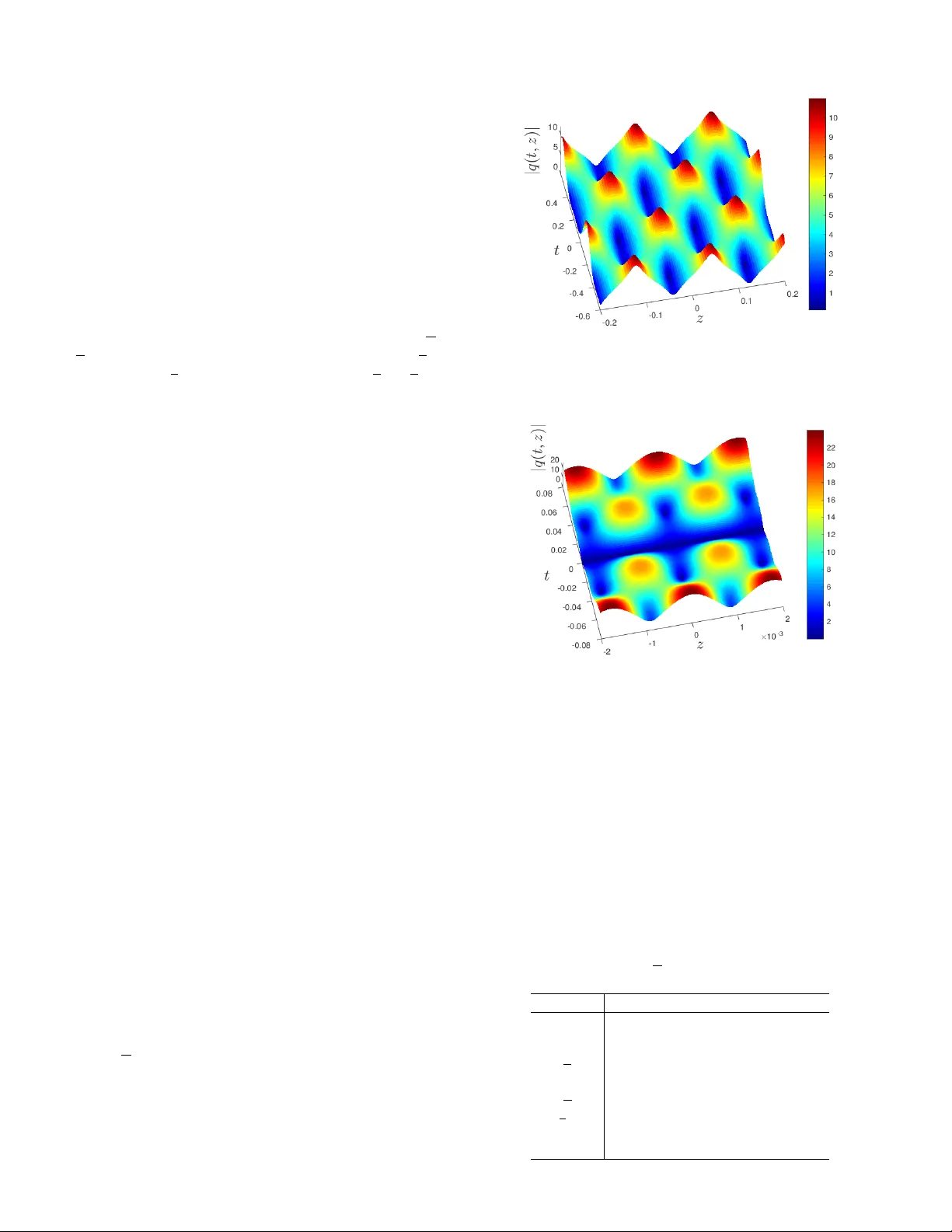
1 Data T ransmission based on Exact In v erse P erio dic Nonlinear F ourier T ransform, P art I: Theory Jan-Willem Go ossens, Student Memb er, IEEE, Hartmut Hafermann, Senior Memb er, IEEE and Y v es Jaouën A bstr act —The nonlinear F ourier transform (NFT) decomp oses w a v eforms propagating through optical fib er in to nonlinear degrees of freedom, which are preserv ed during transmission. By enco ding informa- tion on the nonlinear sp ectrum, a transmission sc heme inheren tly compatible with the nonlinear fib er is ob- tained. Despite p oten tial adv antages, the perio dic NFT (PNFT) has b een studied less compared to its counter- part based on v anishing b oundary conditions, due to the mathematical complexit y of the inv erse transform. In this pap er w e extract the theory of the algebro- geometric in tegration metho d underlying the in v erse PNFT from the literature, and tailor it to the com- m unication problem. W e pro vide a complete algorithm to compute the inv erse PNFT. As an application, we emplo y the algorithm to design a no v el mo dulation sc heme called nonlinear frequency amplitude mo du- lation, where four differen t nonlinear frequencies are mo dulated independently . Finally we provide tw o fur- ther modulation sc hemes that may b e considered in future researc h. The algorithm is further applied in P art I I of this pap er to the design of a PNFT-based comm unication exp eriment. I. Intr oduction N ONLINEAR F ourier transform (NFT) based com- m unication is considered a promising route to address p erformance degradation of data transmission caused by nonlinear in terference in optical fib er [1]. In con- trast to mitigating or comp ensating nonlinear effects, they b ecome an integral part of the signal design. Discov ered in the sixties [2], the NFT — also kno wn as the in verse scattering transform in the mathematical physics context — provides a to ol to solve a wide class of nonlinear partial differen tial equations (the class of integrable equations [3]) analytically . This includes the nonlinear Schrödinger equa- tion (NLSE), whic h describ es the space-time ev olution of the en v elop e of the carrier in optical fib er [4]. Even though signal ev olution in the time-domain in presence of strong nonlinearit y is complex, the ev olution of the nonlinear sp ectrum of the NFT is simpler. When nonlinear degrees of freedom are mo dulated, their recov ery at the receiver remains straightforw ard. Most of the researc h so far has focused on the NFT in its con v entional formulation with v anishing b oundary conditions. In this approac h, signals m ust deca y suffi- cien tly rapidly and b e transmitted in burst mo de, that is, J.-W. Goossens and H. Hafermann are with the Optical Communi- cation T echnology Lab, Paris Research Center, Hua wei T echnologies F rance, 92100 Boulogne-Billancourt, F rance J.-W. Goossens and Y. Jaouën are with L TCI, T élécom Paris, Université Paris-Sacla y , 91120 Palaiseau, F rance b e separated by zero-padding guard interv als to account for disp ersion induced signal broadening. Since its initial prop osal [5]–[7], the application of the NFT to the commu- nication problem has seen progress on several fron ts. This includes the developmen t of techniques to precisely control the time-duration of a signal through b-modulation [8], disp ersion pre-comp ensation to reduce the size of the pro- cessing window at the receiv er [9] and the generalization to p olarization division multiplexing [10]–[12]. F easibilit y of these ideas has also been demonstrated in n umerous exp erimen ts [8], [13]–[18], which improv ed asp ects related to the digital signal pro cessing, and culminated in the curren t record exp erimen tal data rate of 220 Gb/s [19]. A p eriodic v ersion of the NFT (PNFT) has b een de- v elop ed from the mid sev en ties. The study of the peri- o dic inv erse scattering problem giv es rise to the algebro- geometric approac h to nonlinear integrable equations and is discussed in detail with example applications in physics in Ref. [20]. It rev eals a close connection b etw een Riemann surfaces and the theory of Ab elian (or hyperelliptic) func- tions. These are generalizations of elliptic functions, and can b e expressed as ratios of homogeneous p olynomials 1 of the Riemann theta function [21]. The connection b etw een theta functions and nonlinear equations is discussed in Ref. [22]. The impact of the approach on mo dern mathe- matics and theoretical physics is described in Ref. [23] with an emphasis on the historical context. Ref. [24] gives an extensiv e account of nonlinear m ulti-dimensional F ourier analysis in the context of nonlinear o cean w a v es. A first mention of the PNFT in the con text of optical comm unication app ears in Ref. [25], where it is argued that based on the PNFT a discrete version of the NFT should b e obtained. The PNFT has b een suggested to be better suited for the communication problem by W ahls and P o or [26]. Indeed, the PNFT can be considered the more natural generalization of the discrete F ourier transform — whic h also assumes p erio dic b oundary conditions — to nonlinear c hannels. A communication scheme based on exact p eriodic solutions endow ed with a cyclic prefix b ears a close resem blance with orthogonal frequency-division m ultiplexing. In the algebro-geometric approach [20], [27], [28] to the in v erse PNFT, exact solutions to the NLSE are giv en in terms of an analytical expression. This provides a num b er of p otential adv antages of the p erio dic ov er the conv en- tional NFT. The analytical form can, for example, b e exploited to adjust certain prop erties of the solution, such 1 Polynomials whose nonzero terms all hav e identical degree. 2 as its temp oral (or spatial) p erio d, whic h we exploit in this pap er. The underlying algebro-geometric structure ma y also provide a means to address the nonlinear m ultiplexing problem, that is, the computation of the sup erp osition of t w o wa veforms. Algebro-geometric reduction [20], where the symmetry of the nonlinear sp ectrum allows one to reduce Ab elian in tegrals and Riemann theta functions to lo w er genera, simplifies computations [29]. F urther adv an- tages that ha ve b een cited [1], [30] include a significant reduction of the p eak to av erage p ow er ratio compared to burst-transmission for PNFT symbols transmitted with a cyclic prefix. F urthermore, all information is enco ded in a single perio d. Time-duration control is hence automati- cally built in to the approach. While the cyclic prefix length dep ends on transmission distance, the pro cessing window at the receiv er is alwa ys equal to one p erio d. Stable fast algorithms to compute the nonlinear main and auxiliary sp ectra (forward PNFT) of a p erio dic wa v e- form are av ailable [26], [30] and a num ber of data transmis- sion sc hemes based on mo dulating a small n um b er of de- grees of freedom ha v e b een prop osed, suc h as transmission of p erturb ed plane-w a v es [30] or soliton-lik e pulses [31]. Algebro-geometric reduction has b een exploited in the comm unication context in Ref. [32] for gen us 2. The generalization to higher genus ho w ever is not straight- forw ard. The first exp erimental demonstration of PNFT- based data transmission w as presented only recently [33]. A complemen tary metho d for the numerical computation of p erio dic solutions (inv erse PNFT) is based on the solution of an asso ciated Riemann-Hilbert problem [31] to obtain perio dic solutions n umerically . The adv antage is a reduction of the computational complexity compared to the algebro-geometric approach emplo y ed in this pa- p er, while the algebro-geometric approach can lev erage adv antages asso ciated with the a v ailability of a solution in analytical form. The numerical computation of solutions within the algebro-geometric approach has b een partially addressed in the literature. An algorithmic approach to the com- putation of p erio d matrices of Riemann surfaces was presen ted in Ref. [34]. An ov erview of further computa- tional approac hes to Riemann surfaces can be found in Ref. [35]. In [36] a numerical approac h to the computation of solutions for real algebraic curves (which corresp ond to the sp ectra of the defo cusing NLSE) has been presen ted. Numerical asp ects of the ev aluation of Riemann theta functions has previously b een studied [21] and efficient soft w are packages are a v ailable [37]. In this pap er, w e develop the algebro-geometric ap- proac h to the inv erse PNFT for the application to the optical communication problem. A t the core of the pap er, w e develop a fully automatized pro cedure to compute the exact solutions based on the algebro-geometric integration metho d. T o the best of our knowledge, this is the first complete algorithm for the in v erse PNFT which, starting from a main sp ectrum, yields all parameters required for the ev aluation of the analytical solution in terms of in tegrals ov er a Riemann surface. W e present an algorithm to obtain a complete set of closed integration paths (the basis of the homology group, or homology basis for short) on the tw o-sheeted Riemann surface, and a formula to ev aluate integrals o ver these paths. Benc hmark results for the in verse PNFT are also provided. As applications, w e discuss three differen t modulation sc hemes based on the approac h. In P art I I of this pap er [38], the obtained algorithm for the inv erse PNFT is utilized to design a con- stellation for the exp erimen tal demonstration of PNFT- based transmission. T ransmission sc hemes based on the PNFT so far are less dev elop ed than for the conv entional counterpart. T o large extent this is due to the mathematical complexity of the inv erse transform. T o reduce this hurdle, we hav e extracted the theory from the specialized mathematical ph ysics literature and formulated it in a unified notation suitable to the comm unication problem. In the Appendix w e briefly in tro duce the mathematical notions underlying the algebro-geometric approach and pro vide a detailed outline of the deriv ation with links to the relev an t refer- ences. Due to space constraints, the deriv ation can neither b e a complete nor a mathematically rigorous exposition including all necessary pro ofs, which would also b e largely redundan t. Instead the purp ose is to sketc h the deriv ation of the formulas required for our w ork and to pro vide the reader with a means to navigate the sp ecialized literature. The pap er is organized as follows: In Section I I we in tro duce the mathematical structure b ehind the PNFT and the definition of the forward transform. The inv erse PNFT is in tro duced in Section I I I. Section IV details the algorithm for the automatic computation of the in v erse PNFT. Section V provides three different applications of the algorithm b efore we conclude the pap er in Section VI. Notation In this pap er we use b oldface A to denote g × g -matrices while A i,j denotes the element of A in ro w i and column j . W e use underlining, V , to denote a g -dimensional column v ector, where V j is the j -th comp onent of that vector. Dif- feren tials are alw ays recognizable by the Leibniz-notation, dψ . The complex conjugate of a complex num b er z is denoted ¯ z , while its real and imaginary part are denoted b y < ( z ) and = ( z ) , respectively . I I. Periodic NFT W e formulate the PNFT for the fo cusing nonlinear Sc hrö dinger equation (NLSE) [1], which describ es the ev olution of ligh t in anomalous disp ersion optical fib er and is given in dimensionless form b y i ∂ q ( t, z ) ∂ z + ∂ 2 q ( t, z ) ∂ t 2 + 2 | q ( t, z ) | 2 q ( t, z ) = 0 . (1) Con trary to most of literature, where the roles of space and time are rev ersed, the ab ov e notation is suitable to the optical c hannel. The NLSE is an integrable non- linear differential equation. In tegrabilit y hinges on the fact that the NLSE arises as the compatibilit y condition 3 ∂ 2 Φ( t, z , λ ) / ( ∂ t∂ z ) = ∂ 2 Φ( t, z , λ ) / ( ∂ z ∂ t ) b etw een tw o lin- e ar partial differential equations [39]: ∂ Φ ∂ t =  − iλσ 3 +  0 q ( t, z ) − ¯ q ( t, z ) 0  Φ = : U ( t, z , λ )Φ , ∂ Φ ∂ z = " − 2 λU + − iq ( t, z ) ¯ q ( t, z ) − ∂ q ( t,z ) ∂ t − ∂ ¯ q ( t,z ) ∂ t iq ( t, z ) ¯ q ( t, z ) , !# Φ , σ 3 =  1 0 0 − 1  , Φ(0 , 0 , λ ) =  1 0 0 1  . (2) These equations can be understo o d as a scattering prob- lem in whic h q ( t, z ) takes on the role of a p otential. In the context of the algebro-geometric approach, the literature often formulates the PNFT for the so-called coupled nonlinear Schrödinger equation [20], [40] (not to b e confused with the Manak ov equation), of whic h the fo cusing NLSE is a sp ecial case. F or a time-p erio dic signal with p erio d T , q ( t, z ) = q ( t + T , z ) , the columns of Φ b ecome Blo ch functions 2 , and the main sp ectrum is giv en by those v alues λ j for which the Blo c h functions b ecome (anti-)perio dic. A different wa y to state this is that the main sp ectrum of the PNFT is giv en b y those λ j for which the monodromy matrix M , M ( t, z , λ ) := Φ( t + T , z , λ )Φ − 1 ( t, z , λ ) , (3) has eigenv alues ± 1 [28, App. A]. The mono drom y matrix M relates a solution of Eq. (2) at time t to a solution after precisely one p erio d at time t + T . The main sp ectrum alwa ys consists of complex con- jugate pairs b ecause the op erator U ( t, z , λ ) is skew- Hermitian [27]. It can therefore also be describ ed by the g + 1 p oints in the spectrum with p ositive imaginary part. When = ( λ j ) = 0 , the eigenv alue is a double p oint, whic h does not con tribute to the dynamics of q ( t, z ) [26]. The dynamics of the w a v e are captured b y the time- and space-dep enden t auxiliary sp ectrum. It is determined by the p ositions µ j ( t, z ) where the off-diagonal element M 1 , 2 of the mono dromy-matrix v anishes: M 1 , 2 ( t, z , µ j ( t, z )) = M 2 , 1 ( t, z , ¯ µ j ( t, z )) = 0 [27, ab ov e (5.2)]. This definition is due to K otlyaro v and Its [27]. The definition of the auxiliary v ariables is not unique. An alternativ e set of auxiliary v ariables was giv en by Ma and Ablo witz [42]. This description simplifies the retriev al of q ( t, z ) from the auxiliary parameters, at the cost of a more in v olved evolution of the auxiliary sp ectrum itself. How- ev er, no condition seems to b e known to ensure that such a set of auxiliary parameters corresp onds to a solution of the NLSE [26]. W e will therefore not consider this alternativ e set of auxiliary v ariables. Finite-gap solutions When the main sp ectrum of a wa veform consists of only a finite num b er of non-degenerate points, the w av eform is referred to as a finite-gap or finite-band solution. F or finite-gap solutions, q ( t, z ) and the auxiliary spectrum 2 In solid-state physics, Bloch functions arise as eigenfunctions in the treatment of p erio dic p otentials [41]. µ j ( t, z ) are described by a set of coupled partial differential equations: ∂ µ j ( t, z ) ∂ t = − 2 iσ j q Q 2 g +2 k =1 ( λ k − µ j ( t, z )) Q l 6 = j ( µ j ( t, z ) − µ l ( t, z )) , (4) ∂ log q ( t, z ) ∂ t = 2 i   g X j =1 µ j ( t, z ) − 1 2 2 g +2 X k =1 λ k   , (5) with similar, somewhat more complicated equations for the z -deriv atives (see Ref. [27] and Eqs. (47) and (48) in the App endix). The differen tial equations for µ j ( t, z ) are derived from the ev olution of the monodromy matrix, Eq. (3), which in turn is determined by the scattering problem (2). Although the differen tial equations are de- riv ed for perio dic solutions, it turns out that they also ha v e solutions that are not p eriodic. It has b een shown that these differential equations can b e taken as the defining equations of finite-gap solutions [40], which are not necessarily p erio dic. F or given main sp ectrum λ j , the solution to these equations is fully sp ecified by the initial condition µ j (0 , 0) and q (0 , 0) . The absolute v alue of q (0 , 0) is determined b y the initial condition for the auxiliary sp ectrum, while the phase is arbitrary . Not ev ery choice of auxiliary sp ec- trum corresp onds to a solution of the NLSE. A sufficien t constrain t to guarantee an initial condition for the aux- iliary sp ectrum µ j (0 , 0) to yield a solution is given in App endix H. It w as first realized by Kotly aro v and Its [27] that the auxiliary v ariables ( µ j ( t, z ) , σ j ( t, z )) should b e in terpreted as p oin ts on a Riemann surface (8). I I I. Exact inverse PNFT This section in tro duces the algebro-geometric approac h to the inv erse PNFT. The presen tation requires certain mathematical notions which are detailed in Appendix A. Readers not familiar with these notions are recommended to read App endix A first. The inv erse PNFT is a mapping from the main sp ec- trum λ k and initial conditions for the auxiliary sp ectrum µ j (0 , 0) to a solution of the NLSE q ( t, z ) . As outlined in the Appendix, the in tegration of the partial differen tial equations for µ j ( t, z ) and q ( t, z ) leads to exact solutions of the follo wing form: q ( t, z ) = K 0 θ  1 2 π ( ω t + k z + δ − ) | τ  θ  1 2 π ( ω t + k z + δ + ) | τ  e iω 0 t + ik 0 z , (6) where the Riemann theta function is defined by: θ ( x | τ ) = ∞ X m 1 = −∞ . . . ∞ X m g = −∞ exp( π im T τ m + 2 π im T x ) . (7) It is p erio dic in all comp onents of the vector x with p erio d 1. τ is the p erio d matrix. It is symmetric and has p ositive definite imaginary part, which guaran tees conv ergence of the series in the theta function. All parameters on the 4 righ t-hand side of Eq. (6) are obtained as integrals ov er the Riemann surface Γ defined by Γ : ( ( P , λ ) , P 2 = g +1 Y k =1 ( λ − λ k )( λ − ¯ λ k ) , P, λ ∈ C ) . (8) In particular, the parameters ω j and k j are given by ω j = − 4 π i ( A − 1 ) j,g , (9) k j = − 8 π i " ( A − 1 ) j,g − 1 + 1 2 ( A − 1 ) j,g 2 g +2 X k =1 λ k !# , (10) where ( A − 1 ) j,g − 1 := 0 for g < 2 and A is a g × g matrix determined by A j k = Z a k dU j , j, k = 1 , . . . , g . (11) The dU j are the basis of holomorphic differen tials defined in (41) in App endix A. The integration paths a j form half of the canonical homology basis on the Riemann surface. In terms of the p erio ds of the holomorphic differentials o v er the surface Γ the perio d matrix is defined as: τ = A − 1 B , B j k = Z b k dU j , (12) where the cycles b j form the other half of the homology basis. The parameters δ − and δ + are the only ones dep en- den t on the auxiliary sp ectrum, and are defined as: 1 2 π δ ± j = Z ∞ ± p 0 dψ j − 1 2 τ j j + g X k =1 Z a k dψ k ( p 0 ) Z p 0 p 0 dψ j ( p ) − g X k =1 Z µ k (0 , 0) p 0 dψ j . (13) Here p 0 is an arbitrary base p oint on the Riemann surface. T o ensure the in tegrals in this definition are uniquely defined, none of the paths for the integrals must cross any of the a - or b -cycles. Here crossing means that the path cannot b e deformed contin uously to a v oid the crossing without crossing a branch point. The holomorphic differ- en tials dψ are defined by dψ = A − 1 dU . (14) They form a homology basis which is normalized: their p erio ds ov er the a -cycles give the iden tit y matrix: δ j,k = R a k dψ j . In terms of the normalized differentials, the p erio d matrix is giv en by the b -perio ds: τ j,k = R b k dψ j . It w as pro v en [20, Eq. 4.3.22] that each v alid initial condition for the auxiliary spectrum corresp onds to a v ector δ + with = ( δ + ) = 0 and vice v ersa. Therefore choosing a v ector δ + implicitly fixes the initial condition for the auxiliary sp ectrum (see also App endix F). This condition is simpler to implement than the constraint on the auxiliary sp ec- trum detailed in App endix H. W e exploit this in the phase mo dulation scheme introduced below. Note that δ − j and δ − j + 2 π describ e the exact same solution due to the p erio dicity of the theta function. W e c ho ose δ + j = 0 and obtain δ − j from: 1 2 π ( δ + j − δ − j ) = Z ∞ + ∞ − dψ j , (15) where the path from ∞ − to ∞ + m ust not cross any of the cycles in the homology basis. T o solve the differen tial equations for µ j ( t, z ) and q ( t, z ) w e must also provide an initial v alue q (0 , 0) . The ampli- tude | q (0 , 0) | is fixed b y the implicit c hoice of auxiliary sp ectrum, while the phase of q (0 , 0) , and that of q ( t, z ) in general, is a free parameter [27]. This can b e seen from the fact that Eq. (5) only pro vides the rate of change of q . When q ( t, z ) is a solution to the NLSE (1), q ( t, z ) e iφ is also a solution. Similarly , the phase of K 0 in Eq. (6) is a free parameter. Finally , the parameters | K 0 | , ω 0 and k 0 are obtained as the subleading terms in an expansion of meromorphic dif- feren tials d Ω j , j = 0 , 1 , 2 in λ around the p oint λ = ∞ [20, Eq. 4.3.6]. They are uniquely defined by the following prop erties (see App endix G and [20, p. 91]): 1) The differentials are normalized: R a j d Ω k = 0 . 2) Their asymptotic b eha vior is given b y: Ω 0 ( p ) = ± (log λ − log( − 1 4 | K 0 | 2 ) 2 + O ( λ − 1 )) , p → ∞ ± , Ω 1 ( p ) = ± ( λ + ω 0 2 + O ( λ − 1 )) , p → ∞ ± , Ω 2 ( p ) = ± (2 λ 2 + k 0 2 + O ( λ − 1 )) , p → ∞ ± . (16) 3) d Ω k has no other singularities. The integral of d Ω k from ∞ − to ∞ + is given by the difference b etw een the limits: Z ∞ + ∞ − d Ω k = lim p →∞ + Ω k ( p ) − lim p →∞ − Ω k ( p ) . (17) Therefore, the subleading terms are formally determined b y (see App endix G): − log( − 1 4 | K 0 | 2 ) = Z ∞ + ∞ − d Ω 0 − 2 Z ∞ 1 1 λ dλ, (18) ω 0 = Z ∞ + ∞ − d Ω 1 − 2 Z ∞ 0 dλ, (19) k 0 = Z ∞ + ∞ − d Ω 2 − 2 Z ∞ 0 4 λdλ. (20) The last in tegral in each equation subtracts the leading div ergence from the first. Its lo w er b oundary is determined suc h that it do es not introduce an additional constant term. IV. Inverse PNFT algorithm In this section we pro vide an algorithm to numerically compute a solution in the form of Eq. (6). The input of this algorithm are the main sp ectrum 3 , { λ j | j = 1 , . . . , 2 g + 2 } , 3 Note that we tec hnically only need to supply half of the sp ectrum, since the sp ectrum comes in complex conjugate pairs. 5 -3 -2 -1 0 1 2 3 Re( 6 ) -6 -4 -2 0 2 4 6 Im( 6 ) Fig. 1. Three differen t steps in the construction of a homology basis. Left: The initial rectangle constructed for a path around the red eigenv alues. The blac k eigen v alues ended up on the inside of the cycle accidentally . Middle: The same path, after the cut-out pro cedure. Right: The full homology basis, including the sheet changes and directions of the different cycles. The dashed and solid parts of the same cycle lie on the different sheets of the Riemann surface. The path to and from ∞ ± is also shown. The lo cation of the branch cuts (vertical black lines) is illustrative and dep ends on the definition of the square ro ot. and a real phase vector δ + . The output is the solution q ( t, z ) corresponding to that main sp ectrum and c hoice of δ + . The computation of the PNFT is divided into the following subtasks: First, obtain a homology basis for the Riemann surface, as well as a path to ∞ ± . Next, compute the parameters defined by (9), (10), (12) and (15) b y numerically integrating their defining integrals ov er these paths. Then ev aluate the integrals ov er the mero- morphic differentials and isolate their subleading b eha vior to obtain | K 0 | , ω 0 and k 0 according to Eqs. (18) to (20). Finally , giv en all parameters, q ( t, z ) m ust b e ev aluated. The ev aluation of the Riemann theta function has b een studied in literature [21] and efficient soft w are packages are av ailable [37]. W e therefore only provide algorithms for the other three steps. A. Computing inte gr ation p aths The first step in obtaining the theta function parameters is the computation of a canonical homology basis. A homology group element (cycle) of the Riemann surface is completely determined by stating which branch p oints λ j are inside it. By taking the following sets as p oin ts inside the cycle for the different basis elements, a homology basis is obtained: a j : { λ 1 , · · · , λ 2 j } , b j : { λ 2 j , λ 2 j +1 } , j = 1 , . . . , g . (21) T o simplify the construction of these cycles, we organize the λ j in an order such that λ 2 j − 1 = ¯ λ 2 j , j = 1 , . . . , g + 1 , (22) |= ( λ 2 j ) | ≤ |= ( λ 2 j +1 ) | , j = 1 , . . . , g, (23) sgn ( = ( λ 2 j )) = sgn = (( λ 2 j +1 )) , j = 1 , . . . , g. (24) The ordering is illustrated for g = 2 in the left panel of Fig. 1. W e construct the individual elemen ts in the homol- ogy basis by a ’cut-out’ pro cedure. W e first determine a cycle in the form of a rectangle that contains all necessary p oin ts, and then cut out an y p oints from the sp ectrum that w ere supp osed to b e outside the cycle, but which ended up on the inside of the original rectangle. W e represent a path γ as an ordered sequence of N w a yp oin ts [ ν 1 , . . . , ν N ] of the λ -co ordinate in the complex plane. The complete description requires the location of the sheet-changes, as describ ed in Sec. IV-B below. The path is obtained b y connecting subsequent p oints by straight lines. A closed path has ν 1 = ν N . As an example we construct a cycle around the p oints in the set ˜ λ in while ensuring that all other branc h p oints are excluded. T o maximize the accuracy of the n umerical in tegration ov er the homology basis, we attempt to stay as far as p ossible from the branch points, since at these p oin ts the in tegrands ha v e a singularit y . W e define  = 1 2 min i,j (max( |< ( λ i − λ j ) | , |= ( λ i − λ j | ))) , whic h is chosen suc h that a square with side length 2  centered around one branc h p oint has a distance of at least  to any other. First, w e find the higher ( H ) and lo w er ( L ) extreme v alues in real ( R ) and imaginary ( I ) part: L R = min j < ( λ j ) − , H R = max j < ( λ j ) + , (25) L I = min j = ( λ in j ) − , H I = max j = ( λ in j ) + . (26) These v alues define the corners of a rectangle: [ L R + iH I , H R + iH I , H R + iL I , L R + iL I ] , whic h is guaran teed to contain all p oints ˜ λ in . Note that the left and right b oundaries are chosen suc h that they enclose al l p oints. The rectangle can also contain additional p oints. By virtue of (21) and (23), the cycles a j con tain the 2 j smallest eigen v alues by imaginary part. The points to b e excluded are therefore already outside the cycle or guaran teed to lie inside a band of width  at the top or b ottom of the rectangle. By virtue of (21) and (24), a b -cycle is alwa ys lo cated on one side of the real axis. Because of (23), w e ha v e for the imaginary part of all other branch points λ i in b j that = λ i ≤ = λ 2 j or = λ i ≥ = λ 2 j +1 . The same conclusion therefore holds for the b -cycles. Assuming the cycle is tra v ersed clo c kwise starting from the top left corner, a p oin t λ / ∈ ˜ λ in near the top is excluded from the cycle by adding the extra wa ypoints [( < ( λ ) −  ) + iH I , ( < ( λ ) −  ) + i ( = ( λ ) −  ) , ( < ( λ ) +  ) + i ( = ( λ ) −  ) , ( < ( λ ) +  ) + iH I )] , 6 Algorithm 1 Construction of homology basis 1: pro cedure HomologyBasis ( ˜ λ ) 2:  ← 1 2 min k,l max( < ( ˜ λ [ k ] − ˜ λ [ l ]) , = ( ˜ λ [ k ] − ˜ λ [ l ])) 3: ˜ a ← {} 4: ˜ b ← {} 5: for j = 1 , . . . , g do : 6: λ in A ← { ˜ λ [1] , . . . , ˜ λ [2 j ] }  Eq. (21) 7: λ in B ← { ˜ λ [2 j ] , ˜ λ [2 j + 1] }  Eq. (21) 8: app end( ˜ a, GetCycle ( ˜ λ in A , ˜ λ,  ) ) 9: app end( ˜ b, GetCycle ( ˜ λ in B , ˜ λ,  ) ) 10: end for 11: return { ˜ a, ˜ b }  Return lists of w aypoints 12: end pro cedure whic h draw a small rectangular path around the p oin t λ at a distance  . An example is pro vided in the first tw o images in Fig. 1. If a p oint outside the cycle lies closer than  to the b oundary , a similar cut-out pro cedure can b e applied to increase the distance of the path to the p oint. This can impro v e the accuracy of the n umerical ev aluation of the differen tials, since they diverge at the branch p oints λ j . The pseudo co de for the algorithm is sho wn in Algo- rithm 1. The tilde denotes arrays. The input is an array of points ordered according to (22) – (24). The output are arrays for for the a - and b -cycles in the homology basis, each containing an ordered set of wa yp oints. The pro cedure GetCycle in Algorithm 2 returns a cycle as an arra y of w a yp oin ts giv en the array of branc h poin ts to b e inside the cycles, the array of all branch p oints and the constant  . It first determines the p oints of the enclosing rectangle and arra ys of points to be excluded at the top and b ottom. These p oints are cut out one b y one in order. Note that according to lines 10 and 13 eigen v alues that are outside the rectangle but within a distance  from its b orders, are also excluded. T o simplify the determination of the direction of the cycles later, it pro v es useful that they only meet in p oin ts, and nev er o v er extended segmen ts. An o verlap of segmen ts b etw een t w o cycles can b e a v oided b y scaling  b y a factor slightly smaller than one and unique to each cycle when dra wing it (lines 2–5, 23–25 and 30–32 in Algorithm 2), while k eeping the original v alue of  when deciding which p oints to exclude (lines 10, 13). Some of the integrals require a path from ∞ − to ∞ + . It must not cross any other cycle in the homology basis (con tin uous deformations that do not cross branc h p oints are allow ed). A path with a single sheet change is obtained b y encircling a single branch p oin t once. Since λ 2 g +2 do es not participate in any other cycle b y construction, a p ossible path is constructed by the following pro cedure: Start with a square cen tered around the p oint λ 2 g +2 with edges of length 2  . Extend this to the real axis at M = max k < ( λ k ) +  b y first mo ving in the p ositive direction parallel to the real axis and then in the imaginary direction tow ards the real axis. Finally include the real axis from M to ∞ . The pseudo co de for the algorithm to obtain Algorithm 2 Construction of closed cycle 1: pro cedure GetCycle ( ˜ λ in , ˜ λ ,  ) 2: H R ← max k ( < ( ˜ λ [ k ])) +  ,  Eq. (25) 3: L R ← min k ( < ( ˜ λ [ k ])) −   Eq. (25) 4: H I ← max k ( = ( ˜ λ in [ k ])) +   Eq. (26) 5: L I ← min k ( = ( ˜ λ in [ k ])) −   Eq. (26) 6: ˜ λ xtop ← {} 7: ˜ λ xbot ← {} 8: for k = 1 , . . . , 2 g + 2 do 9: if ˜ λ [ k ] / ∈ ˜ λ in then 10: if = ( ˜ λ [ k ]) ≥ H I −  and = ( ˜ λ [ k ]) ≤ H I +  then 11: app end ( ˜ λ xtop , ˜ λ [ k ]) 12: end if 13: if = ( ˜ λ [ k ] ≤ L I +  and = ( ˜ λ [ k ]) ≥ L I −  then 14: app end ( ˜ λ xbot , ˜ λ [ k ]) 15: end if 16: end if 17: end for 18: sortAscendingByRealP art ( ˜ λ xtop ) 19: sortDescendingByRealP art ( ˜ λ xbot ) 20: cycle ← [ L R + iH I ]  T op left corner 21: for k = 1 , . . . , size( ˜ λ xtop ) do 22: R ← < ( ˜ λ xtop [ k ]) 23: I ← = ( ˜ λ xtop [ k ]) −  24: app end ( cycle , [ R −  + iH I , R −  + iI ]) 25: app end ( cycle , [ R +  + iI , R +  + iH I ]) 26: end for 27: app end ( cycle , [ H R + iH I , H R + iL I ]) 28: for k = 1 , . . . , size( ˜ λ xbot ) do 29: R ← < ( ˜ λ xbot [ k ]) 30: I ← = ( ˜ λ xbot [ k ]) +  31: app end ( cycle , [ R +  + iL I , R +  + iI ]) 32: app end ( cycle , [ R −  + iI , R −  + iL I ]) 33: end for 34: app end ( cycle , [ L R + iL I , L R + iH I ])  Close cycle 35: return cycle 36: end pro cedure the path up to the p oin t M is pro vided in Algorithm 3. The obtained path is sho wn in the right panel of Fig. 1. B. She et changes and dir e ction of cycles Eac h of the paths w e just computed is determined by the λ -co ordinate. T o mak e sure the P -co ordinate in (8) (see also (40)), on which the differentials also dep end, is con tin uous, we m ust find the places on each path where a sheet change takes place. The p osition of the sheet c hanges dep ends on the sp ecific implementation of the square ro ot. As an example, the con v en tional definition of the square root function alw a ys returns a num ber with p ositiv e real part. Therefore σ c hanges sign on the negativ e real line, that is, when = ( P 2 ) = 0 and < ( P 2 ) < 0 . W e find these p oints by a standard ro ot-finding algorithm for the function = ( P 2 ) on the straigh t line (cycle segmen t) represen ted by its endp oints: [ ν k , ν k +1 ] . This returns a list of points, ˜ z k, 1 , . . . , ˜ z k, ˜ N k , at which = ( P 2 ) = 0 . This list is 7 Algorithm 3 Construction of path from M − to M + 1: pro cedure P a thToM ( ˜ λ ) 2:  ← 1 2 min k,l max( < ( ˜ λ [ k ] − ˜ λ [ l ]) , = ( ˜ λ [ k ] − ˜ λ [ l ])) 3: M ← max k < ( ˜ λ [ k ]) +  4: s ← sign ( = ( ˜ λ [2 g + 2])) 5: R ← < ( ˜ λ [2 g + 2]) 6: I ← = ( ˜ λ [2 g + 2]) 7: path ← [ M , M + i ( I + s ) , R −  + i ( I + s )] 8: app end ( path , [ R −  + i ( I − s ) , R +  + i ( I − s )]) 9: app end ( path , [ R +  + i ( I + s ) , M + i ( I + s ) , M ]) 10: return path 11: end pro cedure filtered to ensure < ( P 2 ) < 0 and that the path crosses a sheet boundary , yielding a list of N k sheet changes z k, 1 , . . . , z k,N k on segment k . T o determine the direction of the cycles and obtain a canonical basis, for eac h j pick a p oint λ that is common to a j and b j . If a j and b j do not cross in λ b ecause they lie on differen t sheets, rev erse all sheet signs of b j . Finally define the direction of b j suc h that the in tersection n um b er a j ◦ b j (44) equals +1 . See Fig. 1 for an example of a canonical basis showing sheet c hanges and direction of cycles. C. Numeric al evaluation of inte gr als over R iemann surfac e All integrals ov er the Riemann surface that arise in the in v erse PNFT can b e written in the form R γ f ( λ ) /P ( λ ) dλ , where γ is a (not necessarily closed) path on the Riemann surface and f ( λ ) is a function of the λ -co ordinate only . The n umerator also dep ends on the sheet index through P ( λ ) , see Eq. (40). T o compute these integrals, we first divide the integration path into N − 1 straight line seg- men ts represented by their resp ectiv e endpoints, [ ν k , ν k +1 ] , k = 1 , . . . , N − 1 . On segment k , we hav e the N k sheet c hanges z k, 1 , . . . , z k,N k , which further divides the path in to segmen ts betw een sheet c hanges. The integral o v er segmen t k is then given by a sum of integrals ov er the set of segments [ ν k , z k, 1 ] , [ z k, 1 , z k, 2 ] , . . . , [ z k,N k , ν k +1 ] . T o accoun t for the sheet changes, eac h integral is multiplied b y the respective sheet sign σ . Defining z k, 0 ≡ ν k and z k,N k +1 ≡ ν k +1 for notati onal con venience, the integral o v er a path γ can b e expressed as: Z γ f ( λ ) P ( λ ) dλ = N − 1 X k =1 N k X l =0 ( − 1) ( P k − 1 m =1 N m )+ l Z z k,l +1 z k,l f ( λ ) σ P ( λ ) dλ, (27) where the sum o v er k sums the con tributions from the N − 1 segmen ts of the path. The sum P k − 1 m =1 N m in the exp onen t keeps track of the num b er of sheet changes that ha v e o ccurred on the previous line segmen ts. Here f ( λ ) and σ P ( λ ) are functions of λ only , see (40). The integrand has singularities at the branch p oints since P ( λ j ) = 0 . The in tegration paths ho w ev er never cross a branch p oint, see Sec. IV-A and App endix A. The resulting in tegrals ov er the complex plane can therefore b e ev aluated b y standard n umerical metho ds. W e can now compute A , B , and δ + − δ − . F rom these τ , k and ω are obtained straightforw ardly . D. Evaluation of | K 0 | , ω 0 and k 0 This leav es the computation of | K 0 | , ω 0 and k 0 , which separates into tw o parts: First we compute the unique normalized differentials d Ω 0 , d Ω 1 and d Ω 2 whic h hav e their asymptotic b eha vior to w ard ∞ ± determined b y Eqs. (16). F rom these differentials we isolate their sublead- ing b ehavior by remo ving the divergence to w ards ∞ ± . The differen tials defined b y [20, b elow Eq. 4.3.5]: d e Ω 0 = λ g P ( λ ) dλ, (28) d e Ω 1 = λ g +1 − d 1 λ g P ( λ ) dλ, (29) d e Ω 2 = 4 λ g +2 − d 1 λ g +1 − d 2 λ g P ( λ ) dλ, (30) d 1 = 1 2   2 g +2 X j =1 λ j   , d 2 = 1 8   2 g +2 X j =1 λ 2 j − 2 2 g +2 X j =1 X k g . The form ula Ω( p ) = Z p p 0 d Ω( p 0 ) (42) defines a multiv alued function called an Ab elian integral on the whole Riemann surface. Note that the integration o v er the path from p 0 to p will in general inv olv e sheet c hanges, whic h ha v e to b e tak en in to accoun t. In the fol- lo wing and in accordance with the literature, we suppress the explicit dep endence on p if no ambiguit y arises. Ab elian in tegrals can b e divided in to three distinct groups: those of the first kind locally corresp ond to holo- morphic functions, and those of the second kind to mero- morphic functions. All others corresp ond to the third kind and usually ha ve logarithmic singularities. The features of Ab elian in tegrals of the first and second kind are com- pletely describ ed by their p erio ds 4 [20, Eq. 2.4.5]. T o sp ec- ify these p erio ds on a surface of gen us g , w e can define a set of 2 g directed distinct closed curv es a 1 , . . . , a g , b 1 , . . . , b g , whic h can neither b e deformed into each other nor shrunk to zero [35, Sec. 1.3.2]. A closed curve is determined by sp ecifying which branch p oin ts are inside it. An integral o v er the curve do es not change its v alue under con tin uous deformations of the curve, which do es not cross any branch p oin ts. I.e., the top ology remains the same. An y closed curv e on the Riemann surface can b e obtained as a linear com bination of these basis elements. The intersection num b er ( a ◦ b ) p of tw o curves crossing in p is giv en b y the sign of the cross product ( v a j × v b j ) z , where the 3 -dimensional tangent v ectors v a j and v b j lie in the direction of a and b in p , with their first comp onent corresp onding to the real direction and their second com- p onen t to the imaginary direction (the third comp onent 4 Additional p eriods associated with the p oles hav e to be in vok ed for Ab elian integrals of the third kind [20, Eq. 2.4.6]. b eing alwa ys zero). The intersection n um b er of a and b is defined as [35, Def. 14] a ◦ b = X p ∈ a ∩ b ( a ◦ b ) p . (43) The basis is referred to as canonical when a ◦ a = 0 , b ◦ b = 0 , a j ◦ b k = δ j k . (44) F or the torus, the homology basis consists of tw o cycles, one encircling the hole the short wa y , while the other go es around it the long w a y , see Fig. 8 (righ t). The A - and B - p erio ds are expressed in terms of Ab elian in tegrals ov er the elements of the homology basis: A j = Z a j d Ω , B j = Z b j d Ω , j = 1 , . . . , g . (45) The Ab elian in tegral Ω in (42) takes an infinite num b er of different v alues at any p oint p on the Riemann surface. Ho w ever it takes a definite v alue at the p oint p mo dulo the p erio ds. The problem of inv erting the Ab elian integrals of the first kind is known as the Jacobi in v ersion problem. F or g = 1 the result is an elliptic function, that is, a doubly p erio dic function of one complex v ariable. As Jacobi rec- ognized [47], for g > 1 the inv ersion must be carried out for all Ab elian integrals of the first kind simultaneously . This leads to the Abelian or hyperelliptic functions, whic h are 2 g -p erio dic generalizations of elliptic functions and dep end on g complex v ariables. The domain of the h yp erelliptic functions is called the Jacobian v ariety and is giv en by the g -dimensional complex space quotien ted by th e p e- rio d lattice generated by the p eriods of the holomorphic differen tials (45) [20]. The mapping from a p oint on the Riemann surface into its Jacobian v ariety is kno wn as the Ab el map . The inv ersion of the Ab el map pro vides the solution to the Jacobi inv ersion problem in terms of the Ab elian functions. They are constructed using the Riemann theta functions. The in v ersion of the Abel map is sketc hed as part of the deriv ation of the exact solutions of the NLSE in App endix D. The connection b et w een nonlinear equations and theta functions is discussed in Ref. [22]. A useful guide to theory of Riemann surfaces in which most of the notions utilized in this App endix are defined, is giv en by [35, Chapter 1]. B. Governing e quations The integrable, fo cusing NLSE [1] in dimensionless form is given by i ∂ q ( t, z ) ∂ z + ∂ 2 q ( t, z ) ∂ t 2 + 2 | q ( t, z ) | 2 q ( t, z ) = 0 . (46) The integrabilit y of this equation hinges on the fact that the NLSE can b e obtained as the compatibilit y condition 14 ∂ 2 Φ( t, z , λ ) / ( ∂ t∂ z ) = ∂ 2 Φ( t, z , λ ) / ( ∂ z ∂ t ) b etw een t w o lin- ear partial differen tial equations: ∂ Φ ∂ t =  − iλσ 3 +  0 q ( t, z ) − ¯ q ( t, z ) 0  Φ = : U ( t, z , λ )Φ , ∂ Φ ∂ z = " − 2 λU + − iq ( t, z ) ¯ q ( t, z ) − ∂ q ( t,z ) ∂ t − ∂ ¯ q ( t,z ) ∂ t iq ( t, z ) ¯ q ( t, z ) , !# Φ , σ 3 =  1 0 0 − 1  , Φ(0 , 0 , λ ) =  1 0 0 1  . (47) The condition holds true if and only if q ( t, z ) is a solution to the NLSE. The analytical expressions for finite-gap solutions are obtained as exact solutions to the partial differential equa- tions (48) [27, Eqs. 5.5, 5.6] and (49) [27, Eqs. 5.7, 5.8] b elo w. These solutions can b e expressed in an analytical form in terms of integrals o ver a Riemann surface. The deriv ation pro vided in this app endix is structured similarly to the deriv ation in [28]. Ho wev er, it is adapted to the optical channel, and pro vides in particular further details obtained from [20] and [27]. The space-time dep endence of any finite-gap solution is go v erned by the follo wing differential equations [27]: ∂ log q ( t, z ) ∂ t =2 i   g X j =1 µ j ( t, z ) − 1 2 2 g +2 X k =1 λ k   , ∂ log q ( t, z ) ∂ z =2 i   X j >k λ j λ k − 3 4 2 g +2 X k =1 λ k ! 2   − 4 i   − 1 2 2 g +2 X k =1 λ k !   g X j =1 µ j ( t, z )   + 1 2      g X j =1 µ j ( t, z )   2 − g X j =1 µ 2 j ( t, z )       . (48) The dynamics of the wa v eform q ( t, z ) are essen tially go v erned by the so-called auxiliary sp ectrum v ariables µ j ( t, z ) , whic h evolv e on the Riemann surface Γ (39). The motion of the auxiliary sp ectrum v ariables is gov- erned by the differen tial equations [27] ∂ µ j ( t, z ) ∂ t = − 2 iσ j q Q 2 g +2 k =1 ( λ k − µ j ( t, z )) Q l 6 = j ( µ j ( t, z ) − µ l ( t, z )) , ∂ µ j ( t, z ) ∂ z = − 2   X l 6 = j µ l ( t, z ) − 1 2 2 g +2 X k =1 λ k   ∂ µ j ( t, z ) ∂ t , (49) Their evolution is completely indep endent of the solution q ( t, z ) , but can b e though t of as driving the ev olution of q ( t, z ) according to abov e equations. The deriv ation essentially pro ceeds as follows. First, the differen tial equation for µ j ( t, z ) , Eq. (49), is integrated exactly . It is sho wn that the Ab el-map, which was first in tro duced in algebraic geometry , linearizes the evolution of the auxiliary sp ectrum. Next, b y using the Cauch y residue theorem, we obtain expressions for P j µ j ( t, z ) and P j µ 2 j ( t, z ) in terms of integrals ov er the Riemann surface. Finally , the expressions for P j µ j ( t, z ) and P j µ 2 j ( t, z ) are inserted in to the differen tial equations (48) for q ( t, z ) after which they can b e solved analytically . Finally , Sec. G sho ws that the integration constan t and tw o further pa- rameters can b e obtained as integrals o v er meromorphic differen tials o ver the Riemann surface. If one is not in- terested in a sp ecific auxiliary sp ectrum, it can b e fixed implictly . The solution is th us obtained through inte grals o v er a Riemann surface defined b y the main sp ectrum. In the deriv ation, several functions and integrals on the Riemann surface Γ are utilized. F or a point p = ( P , λ ) on the Riemann surface, λ ( p ) denotes the λ -coordinate of that p oint. Eac h v alue λ corresp onds to tw o different p oin ts on the surface (+ P, λ ) and ( − P, λ ) . It is common to denote the p oin ts on the Riemann surface by their λ - co ordinate, keeping the sign of P implicit. If necessary we distinguish betw een the tw o p oints on the Riemann surface b y sup erscript, λ ± . C. Inte gr ation of Eq. (49) The Abel map u is defined for an arbitrary reference p oin t p 0 = ( P 0 , λ 0 ) on the Riemann surface as the follo w- ing map from sets of p oints on Γ to C g : u p 0 ( { p k } ) = n X j =1  Z p j p 0 dψ 1 , . . . , Z p j p 0 dψ g  T , (50) where dψ j is a basis of normalized holomorphic differ- en tials as defined in the paper. The notation { p k } is shorthand for { p k | k ∈ 1 , . . . , n } , whic h denotes a set of n arbitrarily num bered p oints on the Riemann surface. Here n is arbitrary . Given a basis of holomorphic differentials defined on the Riemann surface Γ , dU j = λ j − 1 P ( λ ) dλ, j = 1 , . . . , g, (51) the normalized differen tials are defined as dψ j = g X k =1 C j,k dU k , (52) where C = A − 1 and A j,k = Z a k dU j . (53) W e denote by W ( t, z ) the Ab el-map of the auxiliary sp ectrum: W ( t, z ) = u p 0 ( { µ j ( t, z ) } ) . (54) W ev olves linearly as a function of t and z [27]. This is pro v en by computing the deriv ativ e of W j with resp ect to 15 either t or z , as b elow, and showing that it is constant. Us- ing Eq. (52), the comp onents W j ( t, z ) of W are computed explicitly as: W j ( t, z ) = g X k =1 Z µ k ( t,z ) p 0 dψ j = g X k =1 g X l =1 C j,l Z µ k ( t,z ) p 0 λ l − 1 dλ P ( λ ) . (55) The time-deriv ativ e of this vector is giv en by: ∂ ∂ t W j ( t, z ) = g X k =1 g X l =1 C j,l µ l − 1 k ( t, z ) ∂ µ k ( t,z ) ∂ t P ( µ k ( t, z )) . Inserting the deriv ative of µ k ( t, z ) from Eq. (49), this is found to b e equal to: ∂ ∂ t W j ( t, z ) = g X l =1 − 2 iC j,l g X k =1 µ l − 1 k ( t, z ) Q n 6 = k ( µ k ( t, z ) − µ n ( t, z )) . The Cauc hy residue theorem [48] equates the integral of an analytic function o ver a closed path in the complex plane to the sum of the residues of its p oles inside the closed path. Therefore the ab ov e sum ov er k can b e rewritten as a contour integral: I 0 = g X k =1 µ l − 1 k ( t, z ) Q n 6 = k ( µ k ( t, z ) − µ n ( t, z )) = 1 2 π i Z C λ l − 1 dλ Q g n =1 ( λ − µ n ( t, z )) , (56) where C is a con tour in the complex plane that encloses the p oles µ k . On the other hand this integral can also b e ev aluated b y reversing the direction of the con tour, which pic ks up the residue at λ = ∞ . The latter can be done by c hange of v ariables v = 1 /λ , which transforms the differential according to dv = − λ − 2 dλ . Multiplying the n umerator and denominator b y v g yields the follo wing result: I 0 = 1 2 π i Z C 0 v g − l − 1 Q g n (1 − µ n v ) dv . (57) The integrand only has a p ole at v = 0 for l = g . Ev aluating the residue at v = 0 , the integral b ecomes equal to the Kronec ker-delta δ l,g . Therefore the deriv ative of W j with resp ect to t equals ∂ ∂ t W j ( t, z ) = − 2 iC j,g = : 1 2 π ω j . (58) The matrix C is giv en by in tegrals ov er the Riemann surface according to (53) and therefore dep ends on the main spectrum only . Hence it is constant and W j is a linear function of t . A similar, but more inv olved computation [40] allows one to ev aluate the z -deriv ativ e of W : ∂ ∂ z W j ( t, z ) = − 4 i " C j,g − 1 + 1 2 2 N +2 X k =1 λ k ! C j,g # = : 1 2 π k j . (59) In tegrating Eq. (58) and Eq. (59) gives W ( t, z ) = 1 2 π ( ω t + k z + d ) , (60) where the in tegration constan t d is determined by the Ab el-map of the initial v alue of the auxiliary v ariables: d 2 π = u p 0 ( { µ j (0 , 0) } ) . (61) D. A b el map and inversion of the A b el map F or giv en t and z the auxiliary sp ectrum is obtained b y inv erting the Ab el map. This is known as the Jacobi- in v ersion problem and can b e stated as follows: F or a p oin t V in the Jacobian v ariety of Γ find the set { p j } suc h that u p 0 ( { p j } ) = V . Jacobi formally solved this problem by constructing an analytic function whose zero es are precisely the p oints p j . He sho wed that this function is defined b y [35] F ( p ) = θ  u p 0 ( { p } ) − K + V | τ  , (62) where K j = 1 2 τ j j − g X k =1 Z a k dψ k ( p 0 ) Z p 0 p 0 dψ j ( p ) (63) and the g × g p eriod matrix τ is defined as τ ij = g X k =1 ( A − 1 ) i,k B k,j , B k,j = Z b j dU k . (64) Note that here the argument of the Ab el map u only consists of a single point p . The vector K as w ell as the Ab el map dep end on the base p oint p 0 . How ever the deriv atives of F with resp ect to p as w ell as its ro ots are indep enden t of p 0 . This is also true for its T aylor expansion in the neighborho o d of any of its ro ots. Since F is analytic, it is equal to its T a ylor expansion and hence indep endent of p 0 . In the last equation and in the the remainder of the App endix we therefore suppress the dep endence of the Ab el map on p 0 . No w define a function F ( t, z , p ) , b y: F ( t, z , p ) = θ ( u ( { p } ) − K + W ( t, z ) | τ ) , (65) where the Abel map of the auxiliary sp ectrum (60) is inserted in place of V in the defining equation of F , Eq. (62). The function F formally solves the differential equation for µ j ( t, z ) : The µ j ( t, z ) app ear as zero es of F ( t, z , p ) . E. Evaluating the sums over µ j ( t, z ) It is imp ortan t that the differential equations for q ( t, z ) , Eq. (48), only dep end on the µ j ( t, z ) as sums P j µ j ( t, z ) and P j µ 2 j ( t, z ) , since these sums can be rewritten as con tour integrals o ver Γ by means of the Cauc h y residue theorem. The pro cedure is similar to the ev aluation of I 0 ab o v e. W e first construct the con tour integrals and ev aluate them explicitly in terms of loop integrals ov er the Riemann surface. 16 Since F has zero es at µ j ( t, z ) , 1 F dλ = d log( F ) dλ dλ ≡ d log( F ) has first order p oles at µ j ( t, z ) with residue 1. Therefore a meromorphic differen tial with the residues µ j ( t, z ) is giv en b y λ ( p ) d log F ( t, z , p ) . Similarly , λ 2 ( p ) d log F ( t, z , p ) has residues with v alue µ 2 j ( t, z ) . The factors λ and λ 2 ha v e in troduced extra p oles at p = ∞ ± , whose residue m ust b e subtracted, as sho wn b elow. In order to apply the residue theorem, a contour that encloses all the p oles m ust b e obtained. One wa y to construct suc h a con tour is to cut the Riemann surface along the cycles in the homology-basis and to straighten out the resulting surface to obtain a p olygon [35, Sec. 1.3.2]. This so-called canonical dissection is detailed in Ref. [40] and yields a simply connected surface Γ ∗ . This surface contains all p oints of the original Riemann surface exactly once and hence all the p oles µ j ( t, z ) . It can b e sho wn that the b oundary ∂ Γ ∗ of Γ ∗ is given in terms of the homology basis as a 1 b 1 a − 1 1 b − 1 1 . . . a g b g a − 1 g b − 1 g , where e.g. a − 1 1 denotes the same cycle as a 1 , but tra v ersed in opp osite direction. The in tegrals that need to b e ev aluated therefore are the following: I 1 = 1 2 π i Z ∂ Γ ∗ λ d log F ( t, z , p ) , (66) I 2 = 1 2 π i Z ∂ Γ ∗ λ 2 d log F ( t, z , p ) . (67) Based on the residue theorem the P j µ j ( t, z ) and P j µ 2 j ( t, z ) are found to b e: X j µ j ( t, z ) = I 1 − Res ∞ + [ λ ( p ) d log F ( t, z , p )] − Res ∞ − [ λ ( p ) d log F ( t, z , p )] , (68) X j µ 2 j ( t, z ) = I 2 − Res ∞ + [ λ 2 ( p ) d log F ( t, z , p )] − Res ∞ − [ λ 2 ( p ) d log F ( t, z , p )] . (69) W e exemplify the ev aluation of the residue λ ( p ) d log F ( p ) at p = ∞ + . The other computations proceed in the same w a y . First we write λ d log F = λ ( d log F /dλ ) dλ and apply the chain rule: λ ( p ) d log F ( t, z , p ) = g X j =1  λ ( p ) ∂ log F ( t, z , p ) ∂ u j du j ( p ) dλ  dλ = g X j =1 g X k =1  λ ( p ) ∂ log F ( t, z , p ) ∂ u j C j,k λ k − 1 ( p ) dλ P ( λ )  , (70) where ha ve used that the argumen t of the function F , Eq. (65) only dep ends on λ only through the Ab el map, Eq. (50) and that its differentiation with resp ect to λ yields C j,k λ j − 1 /P ( λ ) by virtue of the definition of the normalized differentials, Eqs. (51) and (52). In the limit of λ → ∞ , 1 /P ( λ ) b ecomes λ − g − 1 + O ( λ − g − 2 ) , which means the previous sum approaches: lim p →∞ ± λ ( p ) d log F ( t, z , p ) = lim p →∞ ± g X j =1 g X k =1 [ D j log F ( t, z , p )] C j,k λ k − g − 1 ( p ) dλ. (71) The only term for whic h this expansion has a residue at λ = ∞ is k = g . In that case, the substitution v = 1 /λ is emplo y ed again, to find: Res ∞ + [ λ ( p ) d log F ( t, z , p )] = g X j =1 C j,g ∂ log F ( t, z , ∞ + ) ∂ u j . (72) The righ t hand side of (72) is, up to a multiplicativ e factor, equal to the t -deriv ativ e of F : ∂ ∂ t log F ( t, z , ∞ + ) = − g X j =1 ∂ log F ( t, z , ∞ + ) ∂ u j ∂ W j ∂ t = 2 i g X j =1 ∂ log F ( t, z , ∞ + ) ∂ u j C j,g , (73) where (58) w as used. Com bining Eqs. (72) and (73), one obtains: Res ∞ + [ λ ( p ) d log F ( t, z , p )] = − i 2 ∂ ∂ t log F ( t, z , ∞ + ) . (74) Computing the other residues in a similar fashion and inserting them in to Eqs. (68) and (69) one obtains: X j µ j ( t, z ) = I 1 − i 2 ∂ ∂ t log  F ( t, z , ∞ − ) F ( t, z , ∞ + )  , (75) X j µ 2 j ( t, z ) = I 2 + 1 4 ∂ ∂ t log[ F ( t, z , ∞ + ) F ( t, z , ∞ − )] − i 4 ∂ ∂ z log  F ( t, z , ∞ − ) F ( t, z , ∞ + )  . (76) In this equation I 1 and I 2 remain unknown. They are no w ev aluated b y separating the border ∂ Γ ∗ in to the constituen t a - and b -cycles. If F were single v alued on the surface Γ the contributions of a and a − 1 w ould cancel. Ho w ever, F is not single v alued. While changing the argumen t p by an a -cycle do es not change the v alue of F , 5 c hanging the argumen t p to p 0 b y mo ving it around a b -cycle changes the v alue of F b y F ( t, z , p 0 ) = exp( − 2 π i ( u j ( { p } ) − K j ) − π iτ j j ) F ( t, z , p ) . (77) Consequen tly , the v alue of d log F ( p 0 ) is giv en by: d log F ( t, z , p 0 ) = − 2 π idψ j + d log F ( t, z , p ) . (78) 5 Since the theta function has perio d 1, and the in tegral of the differentials dψ j is precisely 1 on the a -cycles. 17 In the path Γ ∗ , the cycles a j and a − 1 j are separated precisely by the cycle b j for any j . This leads to the follo wing relations for the contributions of sp ecific cycles: Z a j d log F ( t, z , p ) + Z a − 1 j d log F ( t, z , p 0 ) = Z a j 2 π idψ j , Z b j d log F ( t, z , p ) + Z b − 1 j d log F ( t, z , p 0 ) = 0 . By applying these relations to I 1 and I 2 , Eqs. (66) and (67), w e find the following equalities: Z ∂ Γ ∗ λ d log F ( t, z , p ) = X j Z a j 2 π iλdψ j , Z ∂ Γ ∗ λ 2 d log F ( t, z , p ) = X j Z a j 2 π iλ 2 dψ j . F or I 1 and I 2 this yields: I 1 = g X j =1 Z a j λdψ j , (79) I 2 = g X j =1 Z a j λ 2 dψ j , (80) whic h provide I 1 and I 2 in terms of integrals o v er the Riemann surface. By inserting (79) and (80) into Eqs. (75) and (76), this yields an exact expressions for P j µ j ( t, z ) and P j µ 2 j ( t, z ) . F. Inte gr ation of Eq. (48) The expressions for P j µ j ( t, z ) and P j µ 2 j ( t, z ) obtained in the previous section are now inserted in to Eq. (48) to obtain: ∂ log q ( t, z ) ∂ t = ∂ log J ( t, z ) ∂ t + iω 0 , (81) ∂ log q ( t, z ) ∂ z = ∂ log J ( t, z ) ∂ z + ik 0 , (82) where ω 0 is given by ω 0 = 2 I 1 − 2 g +2 X k =1 λ k , (83) and w e ha v e defined J ( t, z ) := F ( t, z , ∞ + ) /F ( t, z , ∞ − ) . The deriv ative of log J in Eq. (82) comes from the second line in (76). The other terms in Eq. (76) and Eq. (48) are gathered in k 0 . Even though the constituents of k 0 dep end on t and z , k 0 has b een prov en to b e constan t [27], see also Sec. G. The explicit expression can b e found in the original deriv ation in the appendix of [28, below Eq. A30]. By integrating Eqs. (81) and (82) simultaneously and inserting the definition of F , Eq. (65), the analytical form of finite-gap solutions to the NLSE q ( t, z ) is obtained: q ( t, z ) = K 0 θ ( r − − K + W ( t, z ) | τ ) θ ( r + − K + W ( t, z ) | τ ) e iω 0 t + ik 0 z = K 0 θ  1 2 π ( ω t + k z + δ − ) | τ  θ  1 2 π ( ω t + k z + δ + ) | τ  e iω 0 t + ik 0 z . (84) Here r ± = u ( {∞ ± } ) (85) is the Ab el map ev aluated at p = ∞ ± . The second line of this relation is found b y inserting W from Eq. (60) and absorbing all constant terms in the phases δ ± according to 1 2 π δ ± = r ± − K + d, (86) whic h, gathering Eqs. (61), (63) and (85) yields 1 2 π δ ± j = Z ∞ ± p 0 dψ j − 1 2 τ j j + g X k =1 Z a k dψ k ( p 0 ) Z p 0 p 0 dψ j ( p ) − g X k =1 Z µ k (0 , 0) p 0 dψ j . (87) F or giv en main spectrum and initial v alue | q (0 , 0) | (the phase of q (0 , 0) is arbitrary), the expression (84) with ω j and k j giv en by Eqs. (58) and (59), respectively , ω 0 giv en by (83), k 0 giv en in [28, below Eq. A30] and the phases δ ± b y (86), in principle completely describ es the corresp onding finite-gap solution. How ev er, its ev aluation is inconv enient for a n um b er of reasons. Firstly , given an initial v alue q (0 , 0) , a compatible initial auxiliary sp ec- trum must b e obtained from the constraint described in App endix A of the paper, whic h inv olves a n umerical searc h procedure. Secondly , b ecause K 0 app ears in (84) as an integration constant, its v alue dep ends on the initial condition q (0 , 0) . Note that while K 0 app ears to dep end on the auxiliary sp ectrum through the ab ov e mentioned con- strain t and (87), it is in fact indep endent of the auxiliary sp ectrum. Note also that the phase of K 0 is arbitrary (see Sec. I I I in the pap er). F urthermore, k 0 is indep endent of t and z , while as mentioned ab ov e, the explicit expression for it contains sev eral parts that explicitly dep end on t and z and in v olv es deriv ativ es with respect to these v ariables. It turns out that finite-gap solutions can b e obtained in a wa y that is computationally muc h simpler, giv en one is not interested in a sp ecific initial auxiliary sp ectrum. In this case, the solution is obtained by pro viding the main sp ectrum and b y computing integrals ov er the associated Riemann surface. It has b een shown [20, Eq. 4.3.22] that an y v alid initial condition for the auxiliary spectrum cor- resp onds to a phase δ + with v anishing imaginary part. Therefore, the auxiliary sp ectrum can b e fixed implicitly b y choosing, e.g., δ + = 0 . According to (87), δ − can then b e obtained from an in tegral ov er the Riemann surface 1 2 π ( δ + j − δ − j ) = Z ∞ + ∞ − dψ j . (88) It remains to determine ω 0 , k 0 and | K 0 | . In the follo wing section it is shown that these parameters can b e computed in terms of integrals ov er meromorphic differentials o v er the Riemann surface Γ . G. Computation of ω 0 , k 0 and | K 0 | The deriv ation provided b elow follows the deriv ation in Sections 4.1 to 4.3 of [20], but the notation is adapted to 18 the optical channel. W e pro ceed as follows: First, the most general expansion of a solution to the scattering problem, Φ( t, z , λ ) is introduced, and it is sho wn ho w to extract q ( t, z ) from this expansion. Next, a metho d is pro vided to obtain exact solutions to the scattering problem, Eq (47). Finally , a method for computing | K 0 | , ω 0 and k 0 is deriv ed. Let Φ( t, z , λ ) denote a matrix-v alued solution to the coupled equations (47). F rom these it follows that the matrix U is giv en by U ( t, z , λ ) = ∂ Φ( t, z , λ ) ∂ t Φ − 1 ( t, z , λ ) . (89) It is shown in Ref. [20] that an y exact solution Φ( t, z , λ ) can b e expanded around λ = ∞ in the follo wing w a y: Φ( t, z , λ ) = " I + ∞ X k =1 Φ k ( t, z ) λ − k # e − iλtσ 3 − 2 iλ 2 z σ 3 C ( λ ) , (90) where I is the identit y matrix and C ( λ ) is an arbitrary in v ertible matrix. The highest order of λ in the deriv ative of Φ is O ( λ ) , so it is necessary to compute the in v erse of Φ − 1 up to first order in λ − 1 in a neigh b orho o d around λ = ∞ : Φ − 1 ( t, z , λ ) = C − 1 ( λ ) e iλtσ 3 +2 iλ 2 z σ 3  I − Φ 1 ( t, z ) λ − 1  + O ( λ − 2 ) . (91) W e also compute the t -deriv ativ e of Φ , up to the constant term: ∂ Φ ∂ t = − iλ  I + Φ 1 ( t, z ) λ − 1  σ 3 e − iλtσ 3 − 2 iλ 2 z σ 3 C ( λ ) + O ( λ − 1 ) . (92) By multiplying the ab ov e tw o results, an expansion of U ( t, z , λ ) is obtained near λ = ∞ : U ( t, z , λ ) = ∂ Φ ∂ t Φ − 1 = − iλσ 3 − i Φ 1 σ 3 + iσ 3 Φ 1 + O ( λ − 1 ) , = − iλσ 3 + i [ σ 3 , Φ 1 ] + O ( λ − 1 ) . (93) where the square brack ets denote the commutator. In the limit λ → ∞ the O ( λ − 1 ) -term v anishes, and (93) b ecomes exact. The comm utator isolates the off-diagonal elemen ts of Φ 1 , which yields lim λ →∞ U ( t, z , λ ) = lim λ →∞  − iλσ 3 +  0 2(Φ 1 ) 1 , 2 − 2(Φ 1 ) 2 , 1 0  . Comparing this U in (47), the following relations for q ( t, z ) are obtained: q ( t, z ) = 2 (Φ 1 ( t, z )) 1 , 2 = 2  ¯ Φ 1 ( t, z )  2 , 1 . (94) F or the remainder of this appendix, t and z can be considered fixed parameters. A function is called mero- morphic when it is holomorphic except on a set of isolated p oles. Φ( t, z , λ ) is meromorphic in the entire complex plane except at λ = ∞ , where it has an essen tial singularit y (as approaching it from different directions yields differen t v alues). Therefore it is completely defined in the en tire complex plane, through its p oles and its asymptotic b e- ha vior around λ = ∞ . Note that in the expansion (90), the p oles can still b e chosen by c hanging the expansion co efficien ts Φ k . One wa y to mak e the choice of p oles of Φ( t, z , λ ) , which is guaranteed to yield a finite-gap solution was pro vided in [20] as follows: Fix a main sp ectrum, and consider the Riemann surface Γ corresp onding to that main sp ectrum. There exists a unique function φ ( t, z , p ) with the follo wing prop erties [20], [49], [50]: • φ ( t, z , p ) is a single-v alued, meromorphic function on Γ \∞ ± . The p oles of φ ( t, z , p ) are given b y the g p oints p j , j = 1 , . . . , p g on Γ . • In the limit of p → ∞ ± , φ ( p ) is given by lim p →∞ − φ ( t, z , p ) = [  1 0  + O ( λ − 1 )] e − iλt − 2 iλ 2 z , (95) lim p →∞ + φ ( t, z , p ) = λ [  0 1  + O ( λ − 1 )] e iλt +2 iλ 2 z . (96) The p ositions of the poles p j are constrained for the NLSE and corresp ond to a sp ecific auxiliary sp ectrum. An analytic expression for φ ( t, z , p ) can b e computed exactly , see Section 2.7 of Ref. [20]. F or the computation of k 0 and ω 0 , w e only need its asymptotic b eha vior. φ ( t, z , p ) is a sp ecial case of a Baker-Akhiezer function, which is a single- v alued function on a Riemann surface with a finite num ber of exp onen tial singularities and p oles. The comp onents φ i , i = 1 , 2 of the v ector v alued function φ can b e separated in to three parts; a meromorphic function f i ( t, z , p ) with p oles at the points p j , an exp onen tial function e R i ( t,z ,p ) , that provides the exp onential divergence to wards ∞ ± ac- cording to Eq. (96), and a normalization constant F i ( t, z ) , indep enden t of p : φ i ( t, z , p ) = F i ( t, z ) f i ( t, z , p ) e R i ( t,z ,p ) . (97) T aking the limit p → ∞ ± in Eq. (97) and comparing to Eq. (96) giv es: F 1 ( t, z ) = 1 f 1 ( t, z , ∞ − ) , F 2 ( t, z ) = 1 f 2 ( t, z , ∞ + ) . (98) Inserting this in Eq. (97) we find φ 1 ( t, z , p ) = f 1 ( t, z , p ) f 1 ( t, z , ∞ − ) e R 1 ( t,z ,p ) , (99) φ 2 ( t, z , p ) = f 2 ( t, z , p ) f 2 ( t, z , ∞ + ) e R 2 ( t,z ,p ) . (100) W e no w com bine t wo copies of φ ( t, z , p ) as Φ( t, z , λ ) =  φ 1 ( t, z , λ − ) φ 1 ( t, z , λ + ) φ 2 ( t, z , λ − ) φ 2 ( t, z , λ + )  (101) Considering the asymptotic b ehavior of this matrix according to (96) and comparing to (90) in this limit, we can read off the matrix C ( λ ) as: C ( λ ) =  1 0 0 λ  . (102) 19 Remo ving the essential singularit y in (90) b y m ultiply- ing with the inv erse of the exp onential and taking the limit λ → ∞ w e find that: lim λ →∞ Φ 1 , 2 ( t, z , λ ) e iλtσ 3 +2 iλ 2 z σ 3 , = lim λ →∞  I + Φ 1 ( t, z ) λ − 1  C ( λ ) , (103) since all other terms in the expansion v anish. T o obtain q ( t, z ) from (94) we need (Φ 1 ( t, z )) 1 , 2 , whic h we can read off from ab o v e equation as q ( t, z ) = lim λ →∞ 2Φ 1 , 2 ( t, z , λ ) e − iλt − 2 iλ 2 z (104) = lim p →∞ + 2 φ 1 ( t, z , p ) e − iλ ( p ) t − 2 iλ 2 ( p ) z , (105) where in the second line we used (101). Inserting the expansion for φ 1 from Eq. (100), and q ( t, z ) from Eq. (84) w e find: lim p →∞ + 2 f 1 ( t, z , p ) f 1 ( t, z , ∞ − ) e R 1 ( t,z ,p ) e − iλ ( p ) t − 2 iλ 2 ( p ) z (106) = K 0 θ  1 2 π ( ω t + k z + δ − ) | τ  θ  1 2 π ( ω t + k z + δ + ) | τ  e iω 0 t + ik 0 z . (107) In order to determine ω 0 and k 0 , w e equate the exp onential terms in this equation: e iω 0 t + ik 0 z = lim p →∞ + e R 1 ( t,z ,p ) e − iλ ( p ) t − 2 iλ 2 ( p ) z . (108) F ormally this has to b e justified by computing the explicit expression for Eq. (97). It can b e found in [20, Eq. 4.1.16]. By comparing (95) with Eq. (99), we can read off R 1 at ∞ − , but we need it at ∞ + . R 1 is a mermorphic function with p oles only at ∞ ± . That means it is completely defined by providing its Lauren t series in a neighborho o d of ∞ − .W e can write R 1 in terms of meromorphic functions for whic h the Lauren t series is known at ∞ − and ∞ + to obtain the v alue of R 1 at ∞ + . F or this purp ose the following meromorphic functions Ω j are introduced, via the meromorphic differentials 6 d Ω j : Ω j ( p ) = Z p p 0 d Ω j . (109) The choice of p 0 do es not influence the asymptotic b eha v- ior as long as p 0 is not a p ole of d Ω j . The asymptotic b eha vior around ∞ ± of these meromorphic functions is c hosen to repro duce the asymptotic behavior of R 1 and R 2 : Ω 0 ( p ) = ± (log λ + O (1)) , p → ∞ ± , (110) Ω 1 ( p ) = ± ( λ + O (1)) , p → ∞ ± , (111) Ω 2 ( p ) = ± (2 λ 2 + O (1)) , p → ∞ ± . (112) The meromorphic differentials d Ω i are uniquely deter- mined giv en that they hav e singularities at λ = ∞ ± , and b y the constraint that their integral ov er the a -cycles is zero (i.e., they are normalized) [35, Theorem 15]. 7 6 The Ω j are defined via the differentials d Ω j , b ecause the differ- entials are single valued on Γ , while their integrals are not. 7 A solution can also be derived without normalizing the Ω j on the a -cycles. The resulting parametrization of the solution to the NLSE how ever is not the same as the one derived here. W e observe that, in the limit p → ∞ − , the following equalit y holds for R 1 (compare Eq. (95) and (97) and Eqs. (110) to (112)). lim p →∞ − i Ω 1 ( p ) t + i Ω 2 ( p ) z = lim p →∞ − R 1 ( t, z , p ) + O (1) . Similarly for R 2 w e find, after replacing λ in (96) with e log λ : lim p →∞ + Ω 0 ( p ) + i Ω 1 ( p ) t + i Ω 2 ( p ) z = lim p →∞ + R 2 ( t, z , p ) + O (1) . Let the subleading terms of the differen tials b e giv en b y 8 : Ω 0 ( p ) = ± (log λ + A 0 2 + O ( λ − 1 )) , p → ∞ ± , (113) Ω 1 ( p ) = ± ( λ + A 1 2 + O ( λ − 1 )) , p → ∞ ± , (114) Ω 2 ( p ) = ± (2 λ 2 + A 2 2 + O ( λ − 1 )) , p → ∞ ± . (115) It remains to relate the constants A i to parameters of the theta function solution. The Ω i defined in Eqs. (110) to (112) contain a nonzero constant con tribution, while the constant contribution in the R i is zero. In the limit of p → ∞ − , R 1 is equal to: R 1 ( t, z , p ) = i Ω 1 ( p ) t + i Ω 2 ( p ) z + iA 1 2 t + iA 2 2 z + O ( λ − 1 ) . (116) Because R 1 ( t, z , p ) is meromorphic, the same expansion holds at ∞ + giving lim p →∞ + R 1 ( t, z , p ) = lim p →∞ +  iλ ( p ) t + 2 iλ 2 ( p ) z  + iA 1 t + iA 2 z . (117) Inserting this result into Eq. (108) yields e i ( ω 0 t + k 0 z ) = e i ( A 1 t + A 2 z ) , (118) whic h identifies ω 0 = A 1 and k 0 = A 2 . A 0 is determined b y rep eating the same computation for (Φ 1 ) 2 , 1 , for which we obtain equations for both q and ¯ q : q ( t, z ) = 2 lim p →∞ + f 1 ( t, z , p ) f 1 ( t, z , ∞ − ) e i ( ω 0 t + k 0 z ) , ¯ q ( t, z ) = 2 lim p →∞ − f 2 ( t, z , p ) f 2 ( t, z , ∞ + ) e − A 0 − i ( ω 0 t − k 0 z ) . (119) Note that the symmetry of the main sp ectrum under complex conjugation guaran tees that A 0 , A 1 and A 2 are real [20, p. 111]. If A 1 or A 2 w ere not real, this would cause div ergences in ab o v e equation. The deriv ation of the exact form of the functions f 1 and f 2 is rather inv olv ed. It is given in [20, Sec. 2.7]. 8 In principle, the constant contribution dep ends on the initial point p 0 in Eq. (109) and is differen t for the t w o differen t limits p → ∞ ± . Since the final results only depend on the difference between the subleading terms at ∞ ± , the definition provided here is sufficiently general, and implicitly fixes the base point p 0 . 20 By inserting them in to (119) and equating q ( t, z ) and the conjugate of q ( t, z ) the following relation is obtained: K 0 2 θ  1 2 π ( ω t + k z + δ + − r ) | τ  θ  1 2 π ( ω t + k z + δ + ) | τ  = − 2 K 0 θ  1 2 π ( ω t + k z + δ + + r ) | τ  θ ( 1 2 π ( ω t + k z + δ + ) | τ ) e − A 0 . (120) Here r = δ + − δ − . By careful consideration of the sym- metry of the main sp ectrum and symmetry of the perio d matrix τ , it is sho wn in section 4.3 of [20] that: θ ( v | τ ) = θ ( v | τ ) . (121) Inserting this in the abov e equation, and utilizing that = ( ω ) = = ( k ) = 0 giv es: K 0 2 θ  1 2 π ( ω t + k z + δ + − r ) | τ  θ ( 1 2 π ( ω t + k z + δ + ) | τ ) = − 2 e − A 0 K 0 θ ( 1 2 π ( ω t + k z + δ + + r ) | τ ) θ ( 1 2 π ( ω t + k z + δ + ) | τ ) . (122) This equalit y can only hold for all t and z when all prefactors are equal, and the theta function ratios are equal. F or the amplitude K 0 this yields: | K 0 | 2 = − 4 e − A 0 . (123) Finally , the in tegral o v er the differential is expressed in terms of the following limits: Z ∞ + ∞ − d Ω k = lim p →∞ + Ω k ( p ) − lim p →∞ − Ω k ( p ) . (124) Inserting (113)-(115) on the righ t-hand side of this equa- tion, and using A 0 = − log( −| K 0 | 2 / 4) , A 1 = ω 0 , A 2 = k 0 , one obtains the following relations: − log( − 1 4 | K 0 | 2 ) = Z ∞ + ∞ − d Ω 0 − 2 Z ∞ 1 1 λ dλ, (125) ω 0 = Z ∞ + ∞ − d Ω 1 − 2 Z ∞ 0 dλ, (126) k 0 = Z ∞ + ∞ − d Ω 2 − 2 Z ∞ 0 4 λdλ. (127) The last in tegral in each equation subtracts the leading div ergence in the first. Its low er b oundary is c hosen suc h that it do es not in tro duce a non-zero constant term. F or the vectors δ and r , Eq. (122) leads to the following constrain ts: δ + = δ + + 2 π N , (128) r = − r + 2 π M . (129) where N and M are both arbitrary vectors of in tegers. Due to the perio dicity of the theta function, every vector N and M corresp onds to the same solution of the NLSE. The second constrain t can b e rewritten as < ( r ) = π M . (130) In practice this is already satisfied due to the symmetry of the main sp ectrum, see the analysis in [20, Sec. 4.3.2]. It can be used to v erify if r is prop erly computed. In the first constraint, an arbitrary v alue can b e chosen for N . F or N j = 0 , this gives the constraint = ( δ + ) = 0 . F rom this deriv ation it can not b e seen that all finite-gap solutions are obtained by c ho osing a main sp ectrum and a real v ector δ + . This can b e seen from the original deriv ation in [20, Sec. 4.3.2]. The deriv ation in this Appendix provides the complete description of finite-gap solutions in terms of integrals o v er a Riemann surface defined by the main sp ectrum. T o summarize, the analytical expression is given by Eq. (84), where the perio d matrix τ is defined in (64), ω in (58), k in (59) and the phases are determined by (88), provided one sets δ + = 0 . Finally , | K 0 | , ω 0 and k 0 are giv en by Eqs. (125)-(127). H. Constr aint on the auxiliary sp e ctrum Giv en a main sp ectrum λ k , k = 1 , . . . , 2 g + 2 , not every initial auxiliary sp ectrum ( µ j (0 , 0) , σ j (0 , 0)) , j = 1 , . . . , g and initial condition q (0 , 0) corresp ond to a v alid initial condition for the solution of the NLSE. The constraint to obtaining a solution to the NLSE w as first given in [40], and is rep eated here. Let P ( λ ) b e defined as in Eq. (40). Define the function f through: f 2 ( λ ) : = P 2 ( λ ) − | q (0 , 0) | 2 g Y j =1 ( λ − µ j (0 , 0))( λ − ¯ µ j (0 , 0)) . (131) Then the set of µ j (0 , 0) corresp ond to a solution of the NLSE when f ( λ ) is a p olynomial of finite degree. The pro of of this claim is av ailable in App endix 1 of [40]. Note that this constraint do es not provide an explicit expression to compute a v alid auxiliary spectrum. I. Shift of sp e ctrum One prop erty which follows directly from the ev olution equations for q ( t, z ) and µ j ( t, z ) , Eqs. (4) and (5), is that a shift in the linear sp ectrum of a signal corresp onds directly to a shift in the nonlinear sp ectrum. This can b e shown by taking a µ j (0 , 0) , λ j and q (0 , 0) whic h define a solution to the NLSE, and b y considering the shifted sp ectrum: µ j (0 , 0) → µ j (0 , 0) + Λ and λ j → λ j + Λ , with Λ ∈ R . The time deriv ativ e of µ j ( t, z ) [27, (5.8)], Eq. (4), is unc hanged, showing that µ j ( t, 0) → µ j ( t, 0) + Λ for all t . The time-deriv ativ e of log q [27, (5.5)], Eq. (5) pic ks up an extra − 2 i Λ term. Therefore, if q ( t, 0) corresponded to the original signal, the new signal q Λ ( t, 0) is given by q ( t, 0) e − 2 i Λ t . References [1] S. K. T uritsyn, J. E. Prilepsky , S. T. Le, S. W ahls, L. L. F rumin, M. Kamalian, and S. A. Derevyank o, “Nonlinear Fourier trans- form for optical data pro cessing and transmission: adv ances and persp ectives,” Optic a , vol. 4, no. 3, pp. 307–322, 2017. [2] C. S. Gardner, J. M. Greene, M. D. Kruskal, and R. M. Miura, “Method for solving the kortew eg-devries equation,” Phys. R ev. L ett. , vol. 19, pp. 1095–1097, Nov 1967. 21 [3] A. Das, Inte gr able models , vol. 30. W orld scientific, 1989. [4] G. P . Agraw al, “Nonlinear fiber optics,” in Nonline ar Scienc e at the Dawn of the 21st Century , pp. 195–211, Springer, 2000. [5] M. I. Y ousefi and F. R. Ksc hischang, “Information transmission using the nonlinear Fourier transform, part I-I I I,” IEEE T rans- actions on Information The ory , vol. 60, no. 7, pp. 4312–4369, 2014. [6] J. E. Prilepsky , S. A. Derevy ank o, K. J. Blow, I. Gabitov, and S. K. T uritsyn, “Nonlinear inv erse synthesis and eigenv alue division multiplexing in optical fiber c hannels,” Phys. R ev. L ett. , vol. 113, p. 013901, Jul 2014. [7] S. T. Le, J. E. Prilepsky , and S. K. T uritsyn, “Nonlinear inv erse synthesis for high spectral efficiency transmission in optical fibers,” Opt. Expr ess , vol. 22, pp. 26720–26741, Nov 2014. [8] T. Gui, G. Zhou, C. Lu, A. P . T. Lau, and S. W ahls, “Nonlinear frequency division multiplexing with b-mo dulation: shifting the energy barrier,” Optics expr ess , vol. 26, no. 21, pp. 27978–27990, 2018. [9] I. T av akkolnia and M. Safari, “Disp ersion pre-comp ensation for NFT-based optical fiber comm unication systems,” in 2016 Confer ence on L asers and Ele ctr o-Optics (CLEO) , pp. 1–2, IEEE, 2016. [10] J.-W. Go ossens, M. I. Y ousefi, Y. Jaouën, and H. Hafer- mann, “Polarization-division multiplexing based on the nonlin- ear Fourier transform,” Opt. Expr ess , vol. 25, pp. 26437–26452, Oct 2017. [11] S. Gaiarin, A. M. Perego, E. P . da Silv a, F. D. Ros, and D. Zibar, “Dual-polarization nonlinear Fourier transform-based optical communication system,” Optic a , vol. 5, pp. 263–270, Mar 2018. [12] S. Civelli, S. K. T uritsyn, M. Secondini, and J. E. Prilepsky , “Polarization-m ultiplexed nonlinear inv erse synthesis with stan- dard and reduced-complexity NFT pro cessing,” Opt. Expr ess , vol. 26, pp. 17360–17377, Jun 2018. [13] S. T. Le, V. Aref, and H. Buelow, “High sp eed precomp ensated nonlinear frequency-division multiplexed transmissions,” Jour- nal of Lightwave T e chnolo gy , vol. 36, no. 6, pp. 1296–1303, 2017. [14] S. T. Le and H. Buelow, “64 × 0.5 Gbaud nonlinear frequency division multiplexed transmissions with high order mo dulation formats,” Journal of Lightwave T echnolo gy , v ol. 35, no. 17, pp. 3692–3698, 2017. [15] S. T. Le, K. Sc h uh, F. Buchali, and H. Buelo w, “100 gbps b- modulated nonlinear frequency division m ultiplexed transmis- sion,” in Optical Fib er Communic ation Confer enc e , pp. W1G–6, Optical So ciety of America, 2018. [16] V. Aref, S. T. Le, and H. Buelow, “Mo dulation ov er nonlinear Fourier spectrum: Contin uous and discrete sp ectrum,” Journal of Lightwave T e chnolo gy , vol. 36, no. 6, pp. 1289–1295, 2018. [17] S. Gaiarin, F. Da Ros, N. De Renzis, E. P . da Silv a, and D. Zibar, “Dual-p olarization NFDM transmission using dis- tributed Raman amplification and NFT-domain equalization,” IEEE Photonics T e chnolo gy L etters , vol. 30, pp. 1983–1986, Nov 2018. [18] T. Gui, W. A. Gemech u, J. Goossens, M. Song, S. W abnitz, M. I. Y ousefi, H. Hafermann, A. P . T. Lau, and Y. Jaouën, “Polarization-division-m ultiplexed nonlinear frequency division multiplexing,” in 2018 Confer enc e on Lasers and Ele ctr o-Optics (CLEO) , pp. 1–2, May 2018. [19] X. Y angzhang, S. T. Le, V. Aref, H. Buelo w, D. La v ery , and P . Bayv el, “Experimental demonstration of dual-p olarisation NFDM transmission with b-modulation,” IEEE Photonics T echnolo gy L etters , 2019. [20] E. D. Belok olos, A. I. Bob enko, V. Z. Enolski, A. R. Its, and V. B. Matveev, Algebr o-Ge ometric A ppr oach in the The ory of Inte grable Equations . Springer Series in Nonlinear Dynamics, Berlin, Germany: Springer, 1994. [21] B. Deconinc k, M. Heil, A. Bob enko, M. V an Ho eij, and M. Sc hmies, “Computing Riemann theta functions,” Mathemat- ics of Computation , vol. 73, no. 247, pp. 1417–1442, 2004. [22] B. A. Dubrovin, “Theta functions and non-linear equations,” U spekhi Mat. Nauk , vol. 36, no. 2, pp. 11–80, 1981. [23] V. B. Matveev, “30 years of finite-gap integration theory ,” Phil. T rans. R. Soc. A , vol. 366, pp. 837–875, 2008. [24] A. R. Osb orne, Nonline ar Oc e an W aves and the Inverse Sc at- tering T r ansform . New Y ork, NY, USA: Academic, 2010. [25] M. I. Y ousefi, Information tr ansmission using the nonline ar F ourier tr ansform . PhD thesis, Universit y of T oronto, Depart- ment of Electrical and Computer Enginering, 2013. [26] S. W ahls and H. V. P oor, “F ast numerical nonlinear Fourier transform,” IEEE T rans. Inf. Theory , v ol. 61, pp. 6957–6974, 2015. [27] V. K otly arov and A. Its, “Periodic problem for the nonlinear Schrödinger equation,” arXiv preprint , 2014. [28] E. R. T racy and H. H. Chen, “Nonlinear self-modulation: an exactly solv able model,” Phys. R ev. A , v ol. 37, pp. 815–839, 1988. [29] A. O. Smirnov, “Periodic tw o-phase "rogue w av es",” Matem- aticheskie Zametki , vol. 94, pp. 871–883, Jan. 2013. [30] M. Kamalian, J. E. Prilepsky , S. T. Le, and S. K. T uritsyn, “Periodic nonlinear Fourier transform for fiber-optic comm u- nications, Part I-I I: theory and numerical metho ds,” Optics expr ess , vol. 24, no. 16, pp. 18353–18369, 2016. [31] M. Kamalian, A. V asylchenk ov a, D. Shep elsky , J. E. Prilep- sky , and S. K. T uritsyn, “Signal modulation and pro cessing in nonlinear fibre channels by employing the Riemann–Hilb ert problem,” Journal of Lightwave T echnolo gy , vol. 36, no. 24, pp. 5714–5727, 2018. [32] M. Kamalian, A. V asylchenk o v a, J. Prilepsky , D. Shepelsky , and S. T uritsyn, “Comm unication system based on perio dic non- linear fourier transform with exact inv erse transformation,” in 2018 Eur op e an Confer enc e on Optic al Communic ation (ECOC) , pp. 1–3, 2018. [33] J. Go ossens, Y. Jaouen, and H. Hafermann, “Experimental demonstration of data transmission based on the exact inv erse perio dic nonlinear fourier transform,” in 2019 Optic al Fib er Communic ations Confer enc e and Exhibition (OFC) , pp. 1–3, 2019. [34] B. Deconinck and M. v an Ho eij, “Computing Riemann matrices of algebraic curves,” Physica D , vol. 152-153, pp. 28–46, 2001. [35] C. K. A. I. Bob enko, ed., Computational Appr oach to Riemann Surfac es, L e cture Notes in Mathematics , v ol. 2013. Springer, 2011. [36] C. Kalla and C. Klein, “On the numerical ev aluation of algebro-geometric solutions to in tegrable equations,” Nonline ar- ity , vol. 25, pp. 569–596, feb 2012. [37] C. Swierczewski and B. Deconinck, “Computing Riemann theta functions in Sage with applications,” Mathematics and comput- ers in Simulation , vol. 127, pp. 263–272, 2016. [38] J.-W. Goossens, H. Hafermann, and Y. Jaouën, “Data trans- mission based on exact inverse perio dic nonlinear Fourier trans- form, Part I I: W av eform design and exp eriment,” (in prep ar a- tion) , 2019. [39] P . Lax, “In tegrals of nonlinear equations of evolution and soli- tary wa ves,” Comm. Pur e A ppl. Math , vol. 21, no. 5, pp. 467– 490, 1968. [40] E. R. T racy , T opics in Nonline ar W ave The ory with A pplic a- tions . PhD thesis, Universit y of Maryland, 1984. [41] C. Kittel, Intr o duction to Solid State Physics . New Y ork: Wiley , 1996. [42] Y.-C. Ma and M. J. Ablowitz, “The p erio dic cubic Schrödinger equation,” Studies in Applie d Mathematics , vol. 65, no. 2, pp. 113–158, 1981. [43] M. Kamalian, J. E. Prilepsky , S. T. Le, and S. K. T uritsyn, “On the design of NFT-based communication systems with lump ed amplification,” Journal of Lightwave T e chnolo gy , vol. 35, no. 24, pp. 5464–5472, 2017. [44] S. W ahls, S. Chimmalgi, and P . J. Prins, “FNFT: A softw are li- brary for computing nonlinear Fourier transforms,” The journal of Op en Sour ce Softwar e , vol. 3, pp. 597–598, 2018. [45] M. Kamalian, J. E. Prilepsky , S. T. Le, and S. K. T uritsyn, “Spectral efficiency estimation in p erio dic nonlinear fourier transform based comm unication systems,” in 2017 Optical Fib er Communic ations Confer enc e and Exhibition (OFC) , pp. 1–3, 2017. [46] C. T eleman, “Riemann surfaces. ” Lecture notes, 2003. [47] A. I. Markushevich, Intr o duction to the classic al the ory of A belian functions , vol. 96. American Mathematical So c., 2006. [48] I. Bronstein, K. Semendy a y ev, G. Musiol, and H. Mühlig, Hand- b ook of Mathematics . Springer-V erlag Berlin Heidelberg New Y ork, 2004. [49] I. M. Krichev er, “Methods of algebraic geometry in the theory of non-linear equations,” Russian Mathematical Surveys , vol. 32, no. 6, p. 185, 1977. 22 [50] V. Kotly arov and D. Shep elsky , “Planar unimo dular Baker– Akhiezer function for the nonlinear Schrödinger equation,” A nn. Math. Sci. Appl , vol. 2, pp. 343–384, 2017.