Finding and Removing Clever Hans: Using Explanation Methods to Debug and Improve Deep Models

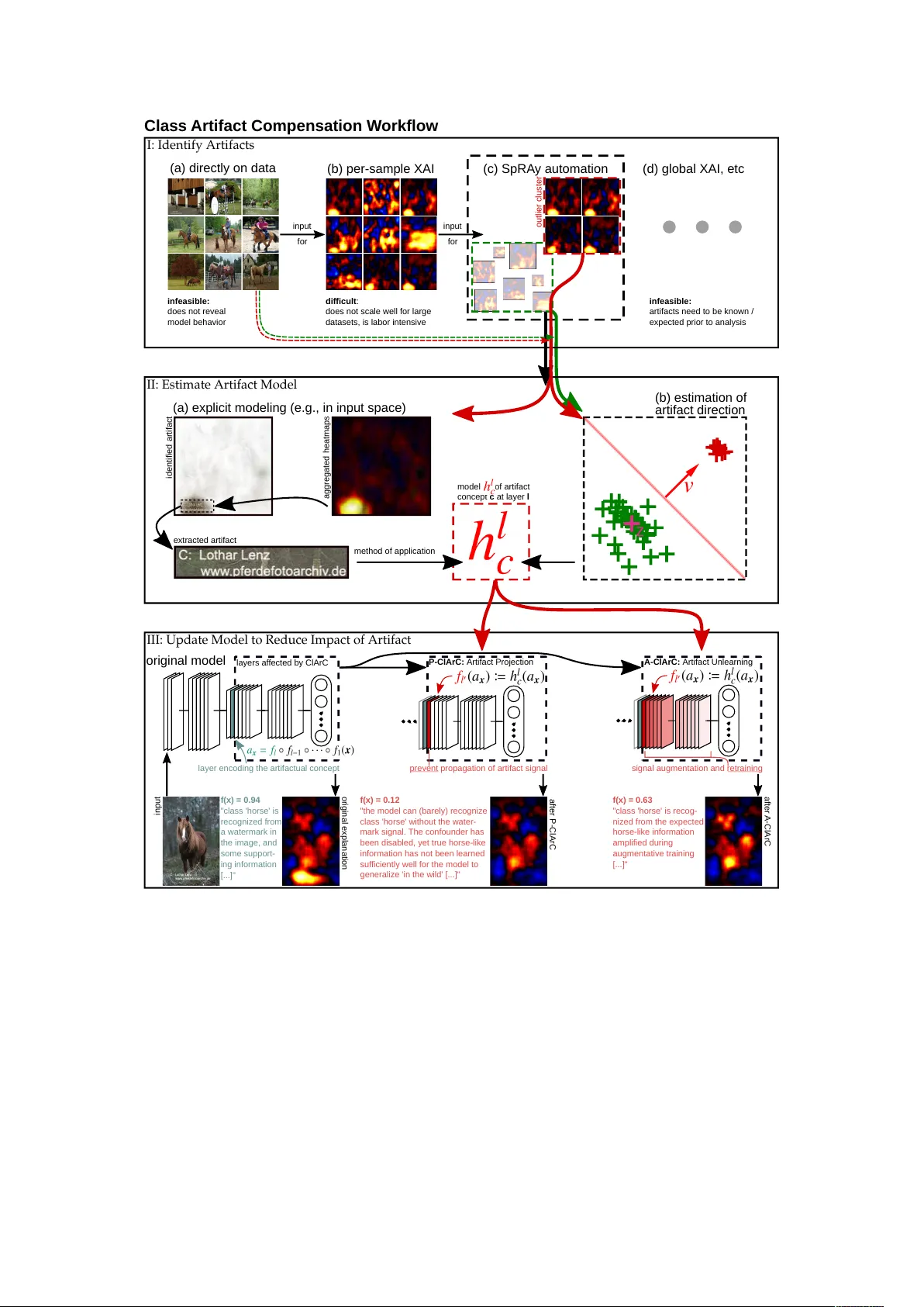
Finding and Remo ving Clev er Hans: Using Explanation Metho ds to Debug and Impro v e Deep Mo dels Christopher J. Anders ∗ 1 , Leander W eb er ∗ 2,3 , Da vid Neumann 3 , W o jciech Samek 3 , Klaus-Rob ert M¨ uller 1,4,5 , and Sebastian Lapusc hkin 3 1 Machine Learning Group, T echnisc he Univ ersit¨ at Berlin, 10587 Berlin, German y 2 Media T echnology Group, T ec hnische Universit¨ at Berlin, 10587 Berlin, German y 3 Department of Artiﬁcial Intelligence, F raunhofer Heinrich Hertz Institute, 10587 Berlin, Germany 4 Department of Artiﬁcial Intelligence, Korea Univ ersity , Seoul 136-713, Korea 5 Max Planck Institut f¨ ur Informatik, 66123 Saarbr ¨ uck en, Germany Decem b er 22, 2020 Abstract Con temp orary learning mo dels for computer vision are t ypically trained on very large (benchmark) datasets with millions of samples. These ma y , ho wev er, contain biases, artifacts, or errors that hav e gone unnoticed and are exploitable b y the mo del. In the worst case, the trained model does not learn a v alid and generalizable strategy to solve the problem it was trained for, and becomes a ‘Clev er-Hans’ predictor that bases its decisions on spurious correlations in the training data, potentially yielding an unrepresen tativ e or unfair, and possibly even hazardous predictor. In this paper, we contribute b y pro viding a comprehensiv e analysis framework based on a scalable statistical analysis of attributions from explanation metho ds for large data corp ora. Based on a recen t tec hnique – Sp ectral Relev ance Analysis – w e propose the following tec hnical con tributions and resulting ﬁndings: (a) a scalable quan tiﬁcation of artifactual and poisoned classes where the machine learning mo dels under study exhibit Clever-Hans behavior, (b) several approaches we collectiv ely denote as Class Artifact Compensation, whic h are able to eﬀectively and signiﬁcantly reduce a mo del’s Clev er Hans b ehavior. I.e., w e are able to un-Hans mo dels trained on (p oisoned) datasets, such as the popular ImageNet data corpus. W e demonstrate that Class Artifact Comp ensation, deﬁned in a simple theoretical framew ork, ma y b e implemented as part of a Neural Netw ork’s training or ﬁne-tuning process, or in a p ost-ho c manner by injecting additional la yers, preven ting any further propagation of undesired Clev er Hans features, into the netw ork architecture. Using our prop osed metho ds, we pro vide qualitative and quan titative analyses of the biases and artifacts in, e.g., the ImageNet dataset, the Adience benchmark dataset of unﬁltered faces and the ISIC 2019 skin lesion analysis dataset. W e demonstrate that these insights can give rise to impro ved, more represen tative and fairer mo dels operating on implicitly cleaned data corpora. Cl ass Arti fact Co mp en sati o n W o rkfl o w I: Artifact Identification out lier clust er unsuspicious samples samples local X A I II: Artifact Model Estimation S p RA y model of art if act ual c layer encoding t he art if act input art if act signal f ilt ering or unlearning t rained model bef ore ClA rC after Cl ArC concept at layer l III: Class Artifact Compensation predict ed f rom: w atermark & horse h o rse o n l y 1 In tro duction Throughout the last decade, Deep Neural Netw orks (DNNs) hav e enabled impressiv e p erformance leaps in a wide range of domains, from solving classiﬁcation problems [1, 2], o ver playing and winning games competitively [3, 4] ∗ contributed equally 1 (some in real time [5, 6]), to enabling the understanding of quantum-c hemical man y-bo dy systems [7] and ﬁnding impro ved solutions to the notoriously diﬃcult task of protein structure prediction [8]. These models are typically (pre-)trained on very large datasets, e.g., ImageNet [9], with millions of samples. Recen tly , it was discov ered that biases, spurious correlations, as well as errors in the training dataset [10] may ha ve a detrimental eﬀect on the training and/or result in ‘Clever-Hans’ predictors [11, 12], which only sup erﬁcially solve the task they ha ve b een trained for, leading to p oten tially unfair and hazardous mo del behavior. Unfortunately , due to the immense size of to day’s datasets, a direct manual inspection and remo v al of artifactual samples can b e regarded hop eless. Analyzing the biases and artifacts in the mo del instead may pro vide insigh ts ab out the training data indirectly . This ho w ever requires an insp ection of the learning mo dels b eyond black b o x mode. Only re cen tly metho ds of eXplainable Artiﬁcial Intelligence (XAI) (cf. [13, 14] for an ov erview) w ere dev el- op ed. They provide deep er insights into ho w a Machine Learning (ML) classiﬁer arrives at its decisions and p oten tially help to unmask Clev er-Hans predictors. XAI methods can be roughly categorized in to t wo groups: metho ds pro viding lo c al (e.g. [15 – 23]) explanations and those providing glob al (e.g. [24 – 27]) explanations [28]. Curren t approaches are of limited use when scaling the search for biases, spurious correlations, and errors in the training dataset, as this would require intense ‘semantic’ human lab or. A recent technique, the Sp ectral Relev ance Analysis (SpRAy) [12], aims to bridge the gap b et ween lo cal and global XAI approac hes b y intro- ducing automation into the analysis of large sets of lo cal explanations. The metho d how ever still inv olv es a considerable amoun t of man ual analyses, esp ecially in context of con temp orary datasets with high n umbers of classes and samples suc h as ImageNet [9]. One of the main goals of ML is to learn accurate decision systems to automate tasks that otherwise ma y only b e solv ed manually . As suc h, sp eciﬁc inference behavior on the a v ailable data often is exp ected from the learned mo dels, e.g., within w ell-deﬁned exp ert domains. As a recen t b ody of research how ev er has demonstrated, deviations from the an ticipated are very lik ely (and must b e exp ected to) app ear in practice. In our pap er, w e prop ose a series of methods constituting a pip eline for the identiﬁcation, description and suppression of those deviations in mo del inference, i.e., a set of to ols to bring the mo del “back on track”: W e introduce a no vel framework we collectively denote as Class Artifact Comp ensation (ClArC) to enable (a) large-scale analyses of a mo del’s inference b eha vior on datasets with hundreds of classes and millions of samples for a semi-automated disco very of undesirable Clev er-Hans eﬀects that are em b edded in to data and model; here w e rely on an extension of SpRAy, which increases the automation p otential on suc h large datasets. (b) In addition, w e provide an intuition for Clever Hans artifacts and the desensitization of a trained model to their inﬂuence. In this manner, ClArC provides (c) a well-con trolled quantitativ e strategy to detect (Figure 1 (Ic) ), mo del and v alidate (Figure 1 (II) ), and consequently remo v e the inﬂuence of such artifacts from the model (Figure 1 (III) ). W e s ho w case the steps of our approach on a mo diﬁed MNIST [29, 30] dataset with color-based Clever Hans (CH) information, the ImageNet [1] dataset, the challenging Adience [31] b enc hmark dataset of unﬁltered faces and the ISIC 2019 [32 – 34] skin lesion analysis dataset, and discuss the in tricacies of (informed in terven tion in) the decision-making of end-to-end learned predictors. These extensiv e analyses allo w interesting ﬁndings that are illuminating b ey ond our sp eciﬁc technical approach. 2 Cl ass Arti fact Co mp en sati o n W o rkfl o w I: Identify Artifacts II: Estimate Artifact Model III: Update Model to Reduce Impact of Artifact (a) direct ly on dat a (b) per-sample X A I (d) global X A I , et c out lier clust er (c) S pRA y aut omat ion input f or input f or (a) explicit modeling (e. g. , in input space) aggregat ed heat maps (b) est imat ion of art if act direct ion ident if ied art if act ext ract ed art if act met hod of applicat ion original model layer encoding t he art if act ual concept layers af f ect ed by ClA rC input original explanat ion f(x) = 0. 94 " class ' horse' is recognized f rom a wat ermark in t he image, and some support - ing inf ormat ion [ . . . ] " model of art if act concept c at layer l signal augment at ion and ret raining A-Cl ArC: A rt if act Unlearning af t er A -ClA rC f(x) = 0. 63 " class ' horse' is recog- nized f rom t he expect ed horse-like inf ormat ion amplif ied during augment at ive t raining [ . . . ] " prevent propagat ion of art if act signal P -Cl ArC: A rt if act P roject ion af t er P -ClA rC f(x) = 0. 12 " t he model can (barely) recognize class ' horse' wit hout t he wat er- mark signal. T he conf ounder has been disabled, yet t rue horse-like inf ormat ion has not been learned suf f icient ly well f or t he model t o generalize ' in t he wild' [ . . . ] " i n feasi b l e: does not reveal model behavior d i ffi cu l t : does not scale well f or large dat aset s, is labor int ensive i n feasi b l e: art if act s need t o be known / expect ed prior t o analysis z Figure 1: The w orkﬂow of our Class Artifact Compensation framework. (I) W e ﬁrst aim to iden tify spurious confounders in the data as learned by the mo del. (Ia) A direct analysis of the training data is infeasible due to the missing corresp ondence to the features used by the mo del during inference. (Ib) Explanations from lo cal XAI methods may provide this information. How ev er, man ual analysis requires the ev aluation of extreme amoun ts of explanations (p er class). (Ic) W e therefore prop ose an automation of this pro cess, based on an extension of the SpRAy [12] algorithm. (Id) While the application of globally op erating XAI tec hniques is disqualiﬁed in the identiﬁcation phase, as here the concepts ev aluated after m ust b e kno wn b eforehand, (II) these tec hniques ﬁnd application in the modeling of an artifact estimator in our approach: (IIa) While an artifact model can b e built explicitly after identiﬁcation, e.g. from exp ert domain knowledge, (IIb) it can also b e learned from represen tative data, e.g. as CA Vs. (III) With a kno wn model of the artifact at the la yer of its most distinct represen tation within the DNN, one can attempt to remov e its inﬂuence on the net w ork. T o this end, w e present the follo wing tw o approaches: P-ClArC aims at the selective deactiv ation of the artifact signal, and, as a largely training-free approac h, leav es the remainder of the model unaltered. A-ClArC on the other hand strategically augments the training data (of all classes) with the artifact signal in order to minimize its class-sp eciﬁc informative v alue, to force the mo del to adapt to other (benign) features in con tinued training. 3 1.1 Related W ork There is an increased aw areness that ML mo dels need to b e interpretable to its users in order to assess the v alidit y of the decision making of the predictor [35, 36], esp ecially in high risk settings, suc h as in medical appli- cations [37 – 41]. T ransparency in mo del predictions could p oint at anomalous or blundering decision b eha vior b efore harm is caused in a later usage as a diagnostic to ol. Consequen tly , numerous approaches to understand asp ects of state of the art Artiﬁcial Intelligence (AI) predictors hav e b een developed in recent y ears (cf. [14] for an o v erview) in the emerging ﬁeld of eXplainable Artiﬁcial In telligence (XAI). In the follo wing paragraphs, we will discuss related w ork by in troducing relev ant researc h w ork and terminology from the ﬁeld of XAI important to this pap er. The Clev er Hans Eﬀect Clev er Hans (CH) was a horse from Berlin, Germany , that allegedly w as able to do math – a media sensation from the early 1900s. Later in 1907 it w as discov ered that Hans w ould read the examinator’s b ody language instead of p erforming arithmetics, and in this manner giv e the right answer but for the wrong reason ∗ [11]. “Clever Hans Strategies” or “Clever Hans Eﬀects” for ML predictors [12, 42] are accordingly named as a homage to this infamous horse, and describ e a prediction making learned and executed based on biases and spurious c or el lations in the training data, instead of v alid (i.e., intended or exp ected) features and relations. As such, there is a notable distinction to mak e betw een the CH artifacts, Backdoor (BD) Attac ks [43, 44] and attac ks based on Adversarial Examples [45]. Adv ersarial attacks are speciﬁcally generated for individual data points in order to cause a misprediction, and are as a consequence ineﬀective when used on other samples. BD A ttacks and CH artifacts on the other hand are systematically learned and exploited b y the mo del. BDs are generally injected with (malicious) in tent during training, into samples of multiple classes via added “trigger patterns” (e.g. a gray pixel at a sp eciﬁc lo cation) while o verriding the the targeted samples’ true training lab els [43, 46]. BDs are usually not part of the original training data an ymore once training is ﬁnished. CH t yp e artifacts, ho wev er, are “naturally o ccurring” phenomena in the training data corpus correlating with only single (or few) ground truth lab els, providing for shortcuts around more complex connections in the training data [47]. In contrast to Backdoor A ttacks, which, if present, cause the mo del to o verride its prediction making on v alid features, CH artifacts almost alw ays app ear alongside benign indicators for a class, and th us exert a signiﬁcan tly weak er inﬂuence on the mo del. F urther, the decision whether a characteristic in the data is indeed a CH, or merely a b enign feature, often is sub ject to the exp ectation of the mo del’s b eha vior and exp ert domain kno wledge [12, 41, 48]. They are consequen tly , in addition to their unexpected nature, more diﬃcult to detect, as exp erimen tally highlighted in Section 3.1. Other than BDs, CH artifacts are part of the features in some of the original training samples, and may thus be identiﬁed during a joint analysis of the a v ailable data and the mo del’s utilization of it, as describ ed throughout this pap er. The particular diﬀerence b et ween datasets with CH artifacts and datasets with BDs is illustrated in Figure 2. In literature, numerous CH strategies hav e b een iden tiﬁed and collected † , e.g., with the help of techniques from XAI, in a surprising num ber of current and former state-of-the-art ML models, in part inv alidating their rep orted (b enc hmark) p erformance as a measure of generalization capability [10, 12, 41, 47 – 51]. Lo cal XAI XAI methods aim at providing transparency to the prediction making of ML mo dels, e.g., for the v alidation of predictions for expert users, or the iden tiﬁcation of failure mo des. Local explanations provide in terpretable feedback on individual predictions of the mo del, and assess the imp ortance of input features w.r.t. sp e ciﬁc samples. Lo cal attributions are commonly presented in the form of heatmaps aligned to the input space, computed, e.g., with (mo diﬁed) bac kpropagation approac hes, such as sensitivity analysis [15, 52], La yer-wise Relev ance Propagation (LRP) [16], Deep T aylor Decomp osition [53], Grad-CAM [18], Integrated Gradien ts [19], SmoothGrad and [54], DeepLIFT [20], whic h require access to the internal parameters of DNN mo dels. Surrogate- and sampling-based approaches, including LIME [21], Prediction Diﬀerence Analysis [22] and Meaningful Perturbations [23] view the mo del as an imp enetrable black b o x and deriv e local explanations via pro xy models and data, at the cost of increased run time and an approximativ e nature of the obtained results. Occlusion analysis [17] follo ws a similar principle b y measuring the eﬀect of the remo v al or perturbation of input features from samples at the mo del output. Shapley v alue based approaches [55, 56] leverage tools from game theory in order to estimate the imp ortance of features to a decision of a mo del. Global XAI Global metho ds aim at obtaining a general understanding ab out a mo del’s sensitivities, learned features and concept encodings. Some approaches operate by assessing the general imp ortance of predetermined ∗ https://en.wikipedia.org/wiki/Clever_Hans † http://tinyurl.com/specification- gaming 4 Cle ver Hans Backdoor 0 1 2 0 2 1 T ar get Figure 2: Diﬀerence b et ween datasets with Clever Hans ( left ) and Backdoor ( right ) artifacts visualized for colored MNIST. The artifact feature that separates aﬄicted samples (red frame) from unaﬀected ones (y ellow frame) here is for both t yp es of artifacts the color blue (diﬀeren t from the standard color white ). In the case of CH artifacts, the artifact feature will only ever app ear in samples alongside features for the a single class. F or BD attacks, the artifact feature app ears in samples among features for all (other) classes except the target class, making the artifact the only discriminative feature in aﬀected samples distinctive for its target class. features, concepts or data transformations b y systematically ev aluating the model’s reaction to v arying exposure thereto, using (larger) sets of real or artiﬁcially generated samples [24 – 27]. Other approaches aim at under- standing predictors b y identifying important neurons and their interactions [57], and visualizing learned feature enco dings by e.g. syn thesizing preferred inputs to hidden ﬁlters within a neural netw ork model, e.g. [58 – 61]. Bridging the gap Both the local and global approaches to XAI suﬀer from a (h uman) in vestigator bias during analysis and thus are on their o wn of only limited use for searc hing and exploring for biases, spurious correlations and errors learned b y the mo del from the training data. Global methods can only measure the impact of pre- determined, exp ected or a priori known features or eﬀects (cf. [26, 27]), whic h limits their applicability when aiming for the discov ery of yet unknown b eha vioral facets of a mo del. Lo cal metho ds, on the other hand, hav e the p oten tial to provide m uch more detailed information p er sample , but the task of compiling information ab out mo del b eha vior o v er thousands (or ev en millions) of samples and explanations is tiring and laborious for a human in v estigator: the success of suc h an analysis dep ends on the examiner’s keen p erception and domain kno wledge, limiting the p oten tial for knowledge discov ery ab out model behavior. A recen t technique, the Spectral Relev ance Analysis (SpRAy) [12], aims at bridging the gap b et ween lo cal and global XAI approaches, by in tro ducing automation in to the analysis of large sets of lo cal explanations. SpRAy has b een applied in a recent set of works, e.g., [12, 48], which how ev er mainly op erate on smaller datasets, each containing only hundreds of samples each. The in [12] describ ed pro cedure how ever still inv olv es a considerable amoun t of manual analyses, esp ecially in con text of con temp orary datasets with high num b ers of classes and samples, such as ImageNet [9]. In our w ork, we purp osefully extend the SpRAy tec hnique and bring it to scale for robustly analyzing extensiv e datasets, in Section 2.4. F eature unlearning The aw areness of CH predictors has in vigorated research with the inten t to improv e mo dels, b y unlearning un wan ted inference patterns. A most naiv e approach to unlearn a concept that can be found in a subset of samples in the training set is to remo v e those samples altogether, and to retrain the mo del from scratch on the reduced training set. While this approach is straigh t forward and easy to implement, it comes a the cost of also removing desirable features the mo del could p ositiv ely b eneﬁt from, along with the c haracteristics in the data deemed problematic. This may b e especially harmful if there are only few training data av ailable to b egin with. F urthermore, in some cases the initial mo del training may hav e b een extremely costly , and an approac h to ﬁne-tune the mo del instead would b e more desirable. Sev eral approac hes hav e thus been dev elop ed to unlearn unw anted predictiv e b eha vior from existing mo d- els [62 – 64] or to guide the mo del during training by providing information ab out the exp ected explana- tions [48, 62, 65]. eXplanatory Interactiv e Learning (XIL) [48, 63] presents lo cal explanations to a human observ er during training, who in turn provides feedbac k to the mo del by replicating samples aﬀected b y CH phenomena and replacing the con tained artifactual features with noise or otherwisely generated patterns. The w ork of Kim et al. [64] introduces a mo del regularization scheme, in whic h an additional “artifact detector” learning sp eciﬁc biasing features is attached to the original predictor. The original mo del is then driven to min- imize the shared information with the dedicated bias predictor, and th us to unlearn to use artifactual features for inference. Ross et al. [65] aim to guide the model tow ards the correct behavior by penalizing high attribu- tion scores in undesired regions by extending the optimization function with a “Right for the Right Reasons 5 (RRR)” loss term. Similarly , Rieger et al. [62] prop ose Contextual Decomp osition Explanation Penalization (CDEP), a metho d for regularizing mo del b ehavior based on explanations obtained from Contextual Decomp o- sition (CD) [66], b y complemen ting the classiﬁcation error of the loss function with an explanation error term. Recen t w ork ho wev er has shown that mo dels can b e manipulated in such a w ay that pro duced attribution maps ma y b e arbitrary , while the prediction of the mo del is unc hanged [67]. Consequen tly , there is no guaran tee that in general unlearning approac hes based on extensions of the loss function eﬀectiv ely correct the mo del’s use of the input features. 2 Metho ds 2.1 Sp ectral Signature F or the detection of BD-t yp e artifacts used b y DNNs, T ran et al. [44] prop ose the Spectral Signature (SpeSig) metho d. Given some dataset X that is p oisoned with a BD and a model f trained on this data, let X y = { x 1 , . . . , x n } b e the subset of samples corresp onding to a target lab el y . T ran et al. [44] apply the follo wing metho d separately for all y in the dataset, since the aim is to identify all (previously unknown) BD samples within X : F or eac h sample x i , the mo del f provides a feature representation a ( x i ). F rom these representations, one computes the co v ariance matrix M = [( a ( x i ) − ˆ a ))( a ( x i ) − ˆ a ) T ] , (1) where ˆ a = 1 n P n i =1 a ( x i ) and n = | X y | . F or eac h sample, an outlier score τ is then computed using the top righ t singular v ector v of M : τ i = (( a ( x i ) − ˆ a ) · v )) 2 (2) Samples with a high τ i are more likely to be outliers, allo wing for the k samples with the largest τ i to b e detected as p oisoned. Note that since Sp eSig detects outliers w.r.t. samples of one class lab el y , the found BDs are usually images that originally b elonged to other classes – and thus do not ﬁt into the manifold of X y . More concisely , Sp eSig do es not detect the p oisoned artifact itself, but the “o dd” samples within X y . T ran et al. [44] then propose to remo ve the detected outliers and retrain the model, thereby defending against the BD attack. In Section 3.1, w e apply the Sp eSig metho d not only to identify BDs, but also on a dataset containing CH artifacts to assert their conceptual diﬀerences. 2.2 Concept Activ ation V ectors Kim et al. [26] introduce CA Vs as a means to pro vide an interpretation of a DNNs internal state in terms of h uman-understandable concepts. Given tw o sets of samples X + and X − , where the samples in X + all exhibit a sp eciﬁc property c (e.g. X + con tains images showing striped ob jects) whic h is not present in X − , a CA V is trained as a linear classiﬁer separating the hidden representations of the samples from X + and X − at some la yer l within the DNN. The thus learned w eight v ector v l c then represen ts the direction in latent space encoding the concept c unique to X + . Kim et al. [26] use CA Vs as directional deriv ativ es in order to test the sensitivities of neural netw ork mo dels w.r.t. to a priori known concepts. W e apply CA Vs tw ofold throughout our pap er. Similar to [26], w e use CA Vs as a means to verify the sensitivit y of the mo del to the CH artifacts, e.g., those identiﬁed via SpRAy, as shown for example in Section 4.2. F urther, w e use CA V directions sp eciﬁc to CH eﬀects in context of the ClArC unlearning framew ork, as a means to remo v e sp eciﬁc b eha vioral facets from the DNN’s inference pro cess. 2.3 La y er-wise Relev ance Propagation La yer-wise Relev ance Propagation LRP [16] is a lo cal XAI approac h rev ersely iterating ov er the la yered structure of a neural net w ork to pro duce an explanation. Consider the neural net work f ( x ) = f L ◦ · · · ◦ f 1 ( x ) . (3) In a forw ard pass, activ ations are computed at each lay er of the neural net work. The activ ation score in the output lay er forms the prediction, which is then backpropagated and redistributed, lay er by lay er, un til the input is reached. The redistribution pro cess follo ws a conserv ation principle analogous to Kirchoﬀ ’s laws in electrical circuits, i.e. all relev ance assigned to any neuron during the process of backpropagation will b e further distributed to w ards its inputs in the la yer b elo w without loss. 6 V arious propagation rules ha ve b een prop osed in literature [16, 68, 69]. F or example, the LRP- γ rule [68] deﬁned as R j ← k = a j ( w j k + γ w + j k ) P 0 ,j a j ( w j k + γ w + j k ) R k , (4) where a j are the lay er’s input activ ation at the j th neuron, w j k the learned parameters mapping the j th input activ ation to the k th la yer output and w + j k = max(0 , w j k ) is the p ositiv e part of the learned weigh ts. The v ariable γ ≥ 0 is a free parameter to tune the decomp osition rule. Equation (4) redistributes R k based on the con tribution of lo wer-la yer neurons to the giv en neuron activ ation, with a preference for positive con tributions o ver negative contributions. This makes it particularly robust and suitable for the low er-lay er con volutions. Other propagation rules suc h as LRP- ε , LRP- αβ or LRP- z B , are suitable for other application scenarios and la yer types [68, 69] and ha ve b een sho wn to w ork well in practice [70]. After the step of relev ance decomp osition, lo wer la yer neuron relev ance is aggregated from incoming relev ance messages as R j = P k R j ← k . F or a technical o verview of LRP including a discussion of the v arious propagation rules and further recen t heuristics, see [68]. In all our exp erimen ts, w e compute LRP attribution scores using LRP- ε (near the mo del output), LRP- γ (in intermediate lay ers) and LRP- z B (near the input), as describ ed in [71]. 2.4 Sp ectral Relev ance Analysis Sp ectral Relev ance Analysis (SpRAy) [12] is a meta-analysis tool for ﬁnding patterns in model behavior, given sets of instance-based explanatory attribution maps. The SpRAy algorithm has its core in Sp ectral Clustering (SC) [72, 73] and – via the use of attribution maps as input – enables the analysis of the input data from the mo del’s persp ective for ﬁnding (hidden) c haracteristics of sp eciﬁc classes, whic h how ever are exploited b y the mo del. The SpRAy algorithm, as in tro duced in [12] initializes by computing the sparse aﬃnit y structure ov er the input attribution maps considering all pair-wise similarities b et ween the given samples. A (normalized, symmetrical and) p ositive semi-deﬁnite graph laplacian L sym [12, 74] is then computed from the aﬃnit y matrix A , and provided as input to SC (cf. [74]). As output, SpRAy yields a sp ectral embedding Φ of the input attributions and the corresponding sp ectrum of eigen v alues Λ = { λ i } i =1 ...q . Lapuschkin et al. [12] follow [74] and (manually) read the structure (i.e. num b er and nesting) of clusters from the eigenv alue sp ectrum Λ, via the sp ectral- or eigen-gap [74], e.g., for ranking a set of analyzed classes w.r.t. to their p oten tial for exhibiting CH phenomena [12]. F or further visual analysis, the aﬃnity matrix A is then used together with a suitable num b er of cluster labels inferred from Λ as a basis for an em b edding in to R 2 , e.g., by using t-SNE [75]. Figure 3 provides an ov erview of the procedure outlined ab ov e, where arrows and symbols in black color describ e the workﬂo w of SpRAy from [12], and arro ws and symbols in red color distinguish our own extensions and adaptations of the algorithm described below. Sp ectral Relev ance Analysis brought to scale W e extend the SpRAy algorithm b y dra wing proper utilit y from the sp ectral em b edding Φ, an in termediate result of the SC algorithm, which so far has remained un used in [12]. While the q ≤ n most signiﬁcant eigenv ectors of the singular v alue decomp osition on the graph laplacian L sym constitute the columns of the ( n × q ) shap ed sp ectral embedding Φ, eac h of the matrix’ ro ws corresp onds to exactly one of the n input attribution maps. W e therefore use the rows of Φ (instead of A ) as an input to mapping and em b edding algorithms suc h as t-SNE [75] or UMAP [76] for pro jecting the spectral analysis results (instead of the prepro cessed data representation A ) in to R 2 for further visual insp ection. Note that the ﬁnal algorithmic step of SC is the assignment of cluster lab els to input samples. F or this purp ose, one usually applies an y other suitable clustering algorithm (e.g. k -Means [77] or DBSCAN [78]) on top of the data represented by the already well-structured em b eddings in Φ. The use of Φ as a source for computing embeddings in R 2 th us leads to a close corresp ondence of the visualized cluster groupings to the assigned cluster lab els. A critical decision in clustering approaches is the num b er of desired clusters. While for small datase ts lik e P ascal VOC [79] it suﬃces to analyze the p er-class eigen-sp ectrum [12]; datasets with a large num b er of classes cannot b e feasibly analyzed by manual comparison and ranking of the eigen-sp ectra of all classes to identify those exhibiting spurious mo del b eha vior. In order to automate this pro cess, we prop ose Fisher Discriminan t Analysis (FDA) to rank all class-wise clusterings b y their resp ectiv e (linear) separability as the quan tity τ . FDA [80, 81] is a widely popular metho d for classiﬁcation as w ell as class- (or cluster-) structure preserving dimensionalit y reduction. FDA ﬁnds an em b edding space by maximizing b et ween-class scatter S ( b ) 7 (d) eigenvalue spectrum inputs with affinity structure (b) (a) Spectral Relevance Analysis Extended Spectral Analysis (e) cluster labels for data (g) local attribution maps visualization embedding (f) (c) separability computation Figure 3: Our extended SpRAy algorithm. ( Black p aths) : Steps follo wed b y the SpRAy pro cedure as deﬁned in [12]. ( R e d p aths) : Our extensions and c hanges to the SpRAy algorithm to increase the automation p oten tial and applicabilit y to very large datasets. (a) F rom a set of lo cal attribution maps, a sparse aﬃnity matrix is computed in (b) . (c) The aﬃnity data is then passed as input for analysis with SC [72, 73] in the form of a p ositiv e semi-deﬁnite graph laplacian, resulting in a sp ectrum of eigenv alues Λ, the sp ectral embedding Φ corresp onding to the input data (see (e) and (g) ), as well as sets of prop osed cluster labels y c . (d) Lapuschkin et al. [12] p erform to a large exten t direct manual analyses on the eigen v alue sp ectrum Λ , within and betw een analyzed classes, for the identiﬁcation of CH b ehavior and distinct cluster groupings, and embed the sparse aﬃnit y structure of the data given the estimated cluster lab els y c for visualization. Our extensions rely on the already expressiv e spectral em b edding Φ (together with cluster lab els y c ) for (e) visualizing the analyzed data groupings, (f ) and the automation and quantiﬁcation of rating clusters and classes for “Clev er Hans’ness” τ , via the computation of separability scores, from, e.g., FD A. and minimizing within-class scatter S ( w ) , giv en b y S ( w ) = K X k =1 X x i ∈ c K k ( x i − µ k )( x i − µ k ) > (5) S ( b ) = K X k =1 ( µ k − µ )( µ k − µ ) > . (6) Here, C K is a clustering with K clusters c K k with k ∈ { 1 , . . . , K } , µ k the sample mean of cluster k and µ the mean o ver the whole set of samples. The solution of FDA can b e understo od as directions of maximal separability b et w een clusterings, and, when normalized and plugged into the original ob jectiv e, gives scores of separability R ( C K ). In our sp eciﬁc use-case, for eac h class we compute separability scores R ( C K ) on the spectral em b edding Φ and each clustering C K in a set of clusterings K = { C K } . W e then deﬁne the class -separability score as τ = 1 | K | X C K ∈ K R ( C K ) , (7) whic h may then b e used to compare classes w.r.t. their “Clever Hans’ness”. In the SpRAy setting, large τ denote outlierness in the predictor’s attribution – as indicators for artifact candidates – whereas low τ do es not indicate any strikingly “irregular” prediction b eha vior. Clearly any algorithmic alternativ es quan tifying the separabilit y of t wo or more sets of lab elled samples may be used as an alternativ e to compute τ , although we see FD A as one of the more in tuitive approaches. Algorithm 1 pro vides a complete algorithmic description of the extended SpRAy tec hnique, while the red arro ws and symbols in Figure 3 distinguish our approac h from SpRAy in [12]. 8 Algorithm 1: Sp ectral Relev ance Analysis Extended Data: Class of in terest y , Data set X = { x 1 , x 2 , ..., x i } Mo del f op erating on X and predicting y Result: Eigen v alues Λ = { λ } , Sp ectral embeddings Φ ∈ R n × q , Clusterings K , Mean separabilit y score τ , Visualization em b eddings V ∈ R 2 /* compute attributions for x ∈ X , using, e.g., LRP */ 1 R = {} ; 2 for x ∈ X do 3 R x = attribution( f , x, y ); 4 R .app end( R x ); 5 end /* Spectral Relevance Analysis */ 6 Φ , Λ , K = SpRAy( R ); /* Compute separability scores given by, e.g., FDA */ 7 for C K ∈ K do 8 S C K = separabilit y(Φ , C K ); 9 end /* compute mean separability score [Eq. (7) ] */ 10 τ = 1 | K | P C K ∈ K S C K ; /* compute embedding visualizations, with e.g., UMAP */ 11 V = visualize em b edding(Φ); 12 return Λ , Φ , K , τ , V 2.5 Class Artifact Comp ensation Assume we ha ve a set of atomic features F . A concept c ∈ 2 F ma y be any combination of atomic features to describ e an abstract prop ert y , where 2 F is the p o wer set of F . W e ma y deﬁne an M -tuple of concepts C = ( c 1 , c 2 , ..., c M ) with c i ∈ 2 F for i ∈ { 1 , ..., M } . Giv en the sup erset of concepts C = S N i =1 c i , assume a set of un tangled data points that can b e constructed b y a com bination of concepts D = { S c ∈ c c | c ∈ 2 C } Eac h un tangled data p oin t α ∈ D is lik e a concept also a com bination of atomic features 2 F . W e may no w, giv en α , construct a signal v ector s ( α ) ∈ { 0 , 1 } M using [ s ( α )] i = δ c i ⊆ α i ∈ { 1 , 2 , ..., M } (8) with the Kronec ker Delta δ , where eac h en try at index i is 1 if c i ⊆ α . In other w ords, s ( α ) is a binary enco ding of α given concepts C . No w assume we ha ve an N-tuple of untangle d datap oin ts D = ( α 1 , α 2 , ..., α N ) with α i ∈ D for i ∈ { 1 , ..., N } . W e may now construct a corresp onding N-tuple of tangle d datap oin ts X = ( x 1 , x 2 , ..., x N ) based on D, where eac h sample x i is a mixture of concepts giv en a pattern matrix A : R N × M x i = As ( α i ) i ∈ { 1 , 2 , ..., N } . (9) Supp ose w e call concept c k at index k ∈ { 1 , 2 , ..., M } an artifact . A set of lab els t i that indicate whether a datap oin t α contains the artifact c k can then b e deﬁned as t i = ( 0 , c k ⊆ α i 1 , c k * α i . (10) Assuming we hav e a function f : R d → R d 0 on the tangled datap oints X , there are tw o questions w e seek answ ers for: 1 - Is f sensitive to artifact c k ? 2 - Ho w can f b e mo diﬁed such that it is insensitive to artifact c k ? Concept Sensitivity of F unctions T o measure the sensitivit y to artifact c k with lab els t i ∈ { 0 , 1 } , one needs to compare the b ehavior of function f on non-artifact samples X − = { x i .i ∈ { 1 , 2 , ..., N }| t i = 0 } and 9 artifact samples X + = { x i .i ∈ { 1 , 2 , ..., N }| t i = 1 } . A naive approac h may b e for example to compare the suﬃcien t statistics µ + = 1 | X + | X x + ∈ X + f ( x + ) and Σ + = 1 | X + | X x + ∈ X + ( f ( x + ) − µ + )( f ( x + ) − µ + ) T (11) with their non-artifact coun ter parts, where | X + | is the cardinalit y of | X + | . This may how ever not give any decisiv e results when the num b er of samples is limited. As another drawbac k, the function may not b e analyzed on a p er-sample basis. Another approac h is to explicitly estimate an artifact model h : R d → R d , which, giv en a non-artifact sample x − i = As ( α i ) with c k * α i pro duces an artifact sample h ( x − i ) ≈ As ( α i ∪ c k ) . (12) W e can formulate the artifact mo del with the ob jectiv e ˆ θ = arg min θ 1 | X − || X + | X x − ∈ X − X x + ∈ X + k h ( x − ; θ ) − x + k 2 (13) where ˆ θ are the optimal h yp erparameters of h . The artifact estimator h is th us the function h with hyperpa- rameters ˆ θ that pro duces the minimal ` 2 -distance betw een mapp ed non-artifact samples h ( x − ) with x − ∈ X − and artifact samples x + with x + ∈ X + . The sensitivity of function f to a concept c k mo deled with h may then b e estimated using S = 1 | X − | X x − ∈ X − k f ( h ( x − ; ˆ θ )) − f ( x − ) k . (14) In tuitively , the addition of a concept may b e more feasible to estimate than the remov al. T ake, for example, the introduction of an opaque watermark in an image. This op eration is not inv ertible as we destro yed the pixel information under the w atermark. While Equations (13) and (14) assume the transformation of a non-artifact sample to an artifact sample in a forwar d artifact mo del, they may equiv alently b e form ulated with a remo v al of the concept in a b ackwar d artifact mo del h b with ˆ θ b = arg min θ 1 | X − || X + | X x − ∈ X − X x + ∈ X + k x − − h b ( x + ; θ ) k 2 (15) The sensitivit y of a function to a concept b ackwar d mo deled b y h b ma y then b e measured using S b = 1 | X + | X x + ∈ X + k f ( h b ( x + ; ˆ θ b )) − f ( x + ) k . (16) Concept Desensitization Dep ending on the type of function f , there ma y be m ultiple possible approac hes to obtain a desensitized function f 0 . If f is for example a function with learned parameters ω , it may be p ossible to learn f 0 b y modifying its training data. If there is enough data a v ailable, the most naiv e approac h to reduce the sensitivity to an artifact c k , is to remov e all samples X + that contain the artifact from training. Dep ending on the amount of av ailable training data, this may not alwa ys b e preferred, since these samples often contain other concepts that ma y b e v aluable for training. In contrast, if the n umber of samples with the artifact concept is larger than the num b er of samples without the artifact concept, one may instead discard all samples without the artifact to obtain an artifact-insensitiv e function. Of course care must b e tak en not to change the data so m uch that the original problem ma y not be solv ed an ymore. A b etter approac h ma y b e is to transform individual samples, suc h that either all samples, or none con tain the artifact. Assuming the addition of an artifact is non-in vertible, w e may prefer to transform all samples to con tain the artifact. This ma y be done by estimating a forwar d artifact mo del h , as deﬁned in Equation (13). The model f may then be trained with the transformed dataset X 0 = ( x 0 1 , x 0 2 , ..., x 0 N ), with: x 0 i = t i x i + (1 − t i ) h ( x i ; ˆ θ ) . (17) A simpliﬁcation arises when the task is to solv e a classiﬁcation problem. Since the model is trained to produce logits for multiple classes, one ma y simply balance the num b er of samples b et ween classes, such that for each class, an identical amount of samples with an artifact are put into the training set by transforming non-artifact samples. 10 Another simpliﬁcation arises when a regularization term is introduced in the artifact mo del, such that h 0 acts as the iden tit y for artifact samples x + ∈ X + with ˆ θ 0 = arg min θ 1 | X − || X + | X x − ∈ X − X x + ∈ X + k h 0 ( x ; θ ) − x + k 2 + λ | X + | X x + ∈ X + k h 0 ( x ; θ ) − x + k 2 . (18) With this regularization term, the error caused b y transforming an already-artifact sample is minimized. Application on Logistic Regression T o build a b etter intuition for the problem, we introduce a logistic regression mo del f ( x ) = σ ( w T x + b ) with sigmoid non-linearity σ ( x ) = 1 1+exp( − x ) . The parameters w and b are obtained b y minimizing the loss function L ( f ) = − 1 N N X i =1 y i log( f ( x i )) + (1 − y i ) log(1 − f ( x i )) + 1 2 γ || w || 2 , (19) with lab els y i ∈ {− 1 , +1 } , where y i = − 1 for samples of class A, using Sto c hastic Gradient Descent (SGD). W e ﬁrst consider the case X + = ∅ , which is visualized in Figure 4 in the panel titled “Clean”. In the panel, we see samples of tw o classes, A (blue) and B (orange), scattered along the y-axis. The green lines visualize the decision hyperplane of f ov er 25 ep o c hs of training. W e can see that the ﬁnal decision h yp erplane (dark green) con verged orthogonal to the signal direction on the y-axis, separating classes A and B p erfectly along their cen ter. In panel “Artifact” of Figure 4, we in tro duce an artifact concept into some of the samples of class A, i.e. | X + | > 0, whic h manifests as an increased v alue along the x-axis. The artifact samples are w ell on the right side of the panel. When now minimizing L ( f ), the con verged decision hyperplane to which w is normal has rotated. While still classifying all the samples correctly , we can visibly see that the introduction of an additional concept has changed the mo del. Based on this observ ation, and the previous discussion, w e in tro duce t wo approac hes under the common name of Class Artifact Comp ensation to comp ensate for class-sp eciﬁc Clever Hans artifacts in SGD-trained inner-pro duct + non-linearit y t yp e mo dels such as logistic regression, or neural netw orks. Artifact Direction Signal Direction Clean Artifact Direction Artifact Artifact Direction = v + v A-ClArC Artifact Direction w T ( I v v T ) x = w T v v T z b z v w T x = b P-ClArC 0 5 10 15 20 25 Decision Boundary at Training Epoch Class A Artifact in A Class B Augmentation in B 0 5 10 15 20 25 Decision Boundary at A-ClArC Epoch Projected Decision Boundary Figure 4: Logistic regression on data with, among p ossibly others, a discriminativ e signal direction and an artifact direction which is only represen ted in one of the tw o classes. The decision-hyperplane is shown o ver the SGD-based training-pro cess of 25 ep ochs in shades of green, with: Clean : no artifact in the data; Artifact : a Clever-Hans artifact in Class A (blue); A-ClArC : with artifact , but training is con tinued with the mean diﬀerence b et ween clean samples and artifact samples in Class A added to some samples of Class B (orange); The in tro duction of an artifact to samples from Class A changes the decision boundary . By in tro ducing the same artifact direction to samples from Class B and retraining, this eﬀect can b e reduced signiﬁcantly . P-ClArC : with artifact , but the mo del is modiﬁed suc h that data points are pro jected on to the h yp erplane at p osition z to whic h the estimated artifact direction v is normal, with k v k = 1 and zero reference z chosen as the mean of clean samples of Class A. The resulting decision hyperplane ignores artifact direction v and sits at the same p osition where the original h yp erplane la y b et ween classes A and B, th us leaving the function output unc hanged for clean samples. Reference z may be c hosen as the mean of b oth clean and artifact samples of Class A to mo ve the resulting decision h yp erplane to wards the middle of b oth classes. 11 Augmen tative Class Artifact Comp ensation The goal of A-C lArC is to augmen t samples in suc h a w ay that the SGD-trained classiﬁer b ecomes insensitiv e to an artifact given artifact lab els t i . Given these lab els, w e estimate a forwar d artifact model h , whic h for our logistic regression toy mo del w e deﬁne as purely additiv e, with: h ( x ) = x + v . (20) Giv en the ob jectiv e from Equation (13), we can see that the optimal v alue for parameter v is v = 1 | X + A | X x + A ∈ X + A x + A − 1 | X − A | X x − A ∈ X − A x − A (21) whic h is the shift b etw een non-artifact samples and artifact samples in class A with with X + A = { x i , i ∈ { 1 , 2 , ..., N }| y i = − 1 ∧ t i = 1 } and X − A = { x i , i ∈ { 1 , 2 , ..., N }| y i = − 1 ∧ t i = 0 } . This is visualized in panel “A-ClArC” in Figure 4. Some samples of class B x B i ∈ { x i , i ∈ { 1 , 2 , ..., N }| y i = +1 } are then mo diﬁed given this artifact mo del with x B i ← h ( x B i ) . (22) The mo diﬁed samples are visualized in Figure 4 with a brighter shade of orange, shifted to the right. The mo del training is then contin ued with the transformed samples, of which the resulting hyperplanes ov er the ep o c hs are visualized as purple lines. W e can observe that the con verged hyperplane resembles the one obtained b y the mo del trained on artifact-free data in panel “Clean” of Figure 4. Bey ond this example, in our exp erimen ts with image data w e assume artifacts are ob jects that are blended in to the image. Therefore w e ma y parameterize the artifact mo del as h ( x ) = diag[ a ] x + (1 − diag[ a ]) z (23) where a ∈ [0 , 1] d is the alpha channel, diag[ a ] : R d × d is a diagonal matrix with diag[ a ] ii = a i with i ∈ { 1 , 2 , ..., d } and z ∈ [0 , 1] d are the RGB v alues of the static image artifact pixels, here each for simplicity represented by a single v alue. By taking CA Vs as a motiv ation, we parameterize the forwar d artifact mo dels in our experiments for feature represen tations in a neural netw ork in an alternative approac h. Explicitly , w e train a linear soft-margin SVM g with hinge-loss L = 1 2 v T v + η X x − ∈ X − max[0 , − v T x − − β ] + X x + ∈ X + max[0 , v T x + + β ] ! (24) with v ∈ R d , regularization constant η and bias term β . W e then design the artifact mo del explicitly b y pushing samples o ver the decision boundary relative to some ﬁxed position z . W e c ho ose z as the mean artifact reference p oin t, with z = 1 | X + | X x + ∈ X + x + . (25) The forwar d artifact model h is then c hosen as an aﬃne transformation h ( x ) = ( I − v v T ) x + v v T z . (26) Pro jective Class Artifact Comp ensation While A-ClArC addresses the problem of desensitization by augmen ting the underlying training data of a prediction mo del f using a forwar d artifact mo del h , P-ClArC instead aims to correct the mo del without retraining by incorporating a b ackwar d artifact mo del h b directly in to the prediction mo del. The approac h is again motiv ated b y CA V and uses the same parameterization for the b ackwar d artifact model as the forwar d model in Equation (26) with h b ( x ) = ( I − v v T ) x + v v T z (27) and v given in Equation (24). Ho wev er, the artifact reference p oin t z here b ecomes the non-artifact reference p oin t, whic h w e no w c ho ose as the center of non-artifact samples X − with z = 1 | X − | X x − ∈ X − x − . (28) This no w mov es all p oin ts along v to a ﬁxed p osition, while leaving all orthogonal directions untouc hed. A strong assumption that is taken for this approach is that really all other concepts are encoded in the directions 12 orthogonal to v . Given this assumption how ever, w e ma y further assume that for all non-artifact examples x − ∈ X − , v T x − ≈ v T z , i.e. there is no v ariance along the artifact CA V. With this, we further obtain ∀ x − ∈ X − : h ( x − ) ≈ x − , i.e. non-artifact samples are approximately unchanged by the b ackwar d artifact mo del h b . Giv en the logistic regression mo del f in Figure 4 in the “P-ClArC” panel, we obtain the mo del f 0 corrected for insensitivit y against the artifact modeled b y h b using f 0 ( x ) = σ ( w T h ( x ) + b ) (29) = σ ( w T ( I − v v T ) | {z } w 0 x + w T v v T z + b | {z } b 0 ) (30) = σ ( w 0 x + b 0 ) . (31) The “P-ClArC” panel shows the decision hyperplane of the original mo del f in green, along with the parameters v and z for the b ackwar d artifact mo del h b , as well as the corrected decision h yp erplane according to Equation (31). Note that the non-artifact reference z is chosen such that the decision hyperplane of f is at the same p osition exactly betw een classes A and B, resulting in a decision hyperplane that is somewhat shifted to wards class A. An alternativ e z may b e c hosen as the mean of all samples of class A to correct for this diﬀerence. How ever, a constrain t of this approac h w ere unc hanged function v alues for non-artifacts, whic h results in this shift. W e can transfer this approach directly to the neural netw ork mo dels in the exp erimen ts section due to their piecewise-linear nature. A detailed Algorithm for b oth A-ClArC and P-ClArC on Neural Netw orks is sho wn in Algorithm 2 under the common name of Class Artifact Comp ensation. Algorithm 2: Class Artifact Comp ensation Data: Samples X = ( x 1 , x 2 , ..., x N ) Lab els T = ( t 1 , t 2 , ..., t N ) describing existence of artifact c in X (cf. Eq. 10) Mo del f op erating on X , with accessible la yer l (and subnet work f l ) F or A-ClArC: data D , ep ochs E for training, p oison rate p ∈ [0 , 1] Result: predictor f 0 desensitized to artifact c /* obtain feature representations of data at layer l */ 1 A l = {} ; 2 for x ∈ X do 3 a x = f l ( x ); 4 A l .app end( a x ); 5 end /* unlearn/deactivate the use of c in f */ 6 if A-ClArC then 7 h l c = forw ard artifact model( A l , T ); /* def. A-ClArC module f l 0 atop layer l , randomly apply artifact transform h l c */ 8 f l 0 ( a x ) : = ( h l c ( a x ) : U [0 , 1] < p a x : else ; 9 f 0 = f L ◦ · · · ◦ f l +1 ◦ f l 0 ◦ f l ◦ · · · ◦ f 1 ( x ); /* unlearn c in layers [ l + 1 , . . . , L ] */ 10 for e ∈ { 1 . . . E } do 11 f 0 .train( D , trainable= [ f l +1 , . . . , f L ]) 12 end 13 else if P-ClA rC then 14 h l c = bac kward artifact mo del( A l , T ); /* def. P-ClArC module f l 0 to suppress c , add on top of layer l */ 15 f l 0 ( a x ) : = h l c ( a x ); 16 f 0 = f L ◦ · · · ◦ f l +1 ◦ f l 0 ◦ f l ◦ · · · ◦ f 1 ( x ); 17 return f 0 13 3 Exp erimen ts – Clev er Hans Identiﬁcation The goal of this section is to explicitly ﬁnd artifact mo dels giv en sets of lab els on our dataset regarding CH artifacts in the training set that were learned b y the analyzed neural netw ork mo del. Therefore, w e start with an exp erimen t to inv estigate the relation and diﬀerence b et ween the detection of CH and BD artifacts within features representations of neural net works [44]. The corresp onding results p oin t us tow ards the necessity of deep er insigh t into the model. Such an insigh t is promised by SpRAy [12], which w e verify subsequen tly on a sp ecially designed version of Colored MNIST using our separability score extension. W e then pro ceed to verify the prop osed separability score τ on a VGG16 mo del [82] trained on ILSVRC2012 b y comparing the scores of classes for which w e ha ve man ually found CH artifact candidates. A description of the training pro cedures and architectures of all mo dels used in this section can b e found in A. W e proceed to visualize some promising CH artifact candidates which we ha ve found in an algorithm-assisted dataset exploration with SpRAy, whic h pro vides us with a set of p ositiv e and negative lab els on samples for each artifact candidate. An exploration is conducted both in input space and feature space in v arious lay ers of our model, for which we provide a comparison on the acquired separability scores. The previously obtained sets of lab els may then b e used to ﬁt or construct an artifact model, w hic h will b e v eriﬁed and used as prerequisite to remov e the corresp onding artifact from a model using A-ClArC and P-ClArC in the following Section 4. 3.1 Relation of Clev er Hans and Bac kdo or Artifacts In this section, we conduct an empirical demonstration on the diﬃculty of detecting CH artifacts compared to BD attacks by analysing a neural net work’s hidden activ ations. W e prepare t wo mo diﬁed instances of the CIF AR-10 dataset [83], one p oisoned by in tro ducing a CH artifact, the other b y adding a BD. In b oth cases, the trigger pattern is a static (3 × 3)-sized grey pixel patch applied to a subset of the training set. F or the CH, this trigger is introduced in to 25% of all samples of class “airplane”. F or the BD, it is introduced into 10% of all samples, with the class lab el of each p oisoned sample c hanged to “airplane”. A simple con volutional netw ork is then trained on eac h training set instance. This netw ork achiev es an unpoisoned v alidation accuracy of 49.1% when trained using the CH artifact, and 46.6% with the BD-p oisoned dataset. As suggested by T ran et al. [44], the Sp eSig metho d (cf. Section 2.1) is used to detect p oisoned samples as outliers. While T ran et al. [44] use this outlier score only to detect BD samples, w e also attempt to detect samples aﬀected by the related CH eﬀect in order to compare these t wo types of dataset p oisoning in terms of their induced feature represen tation. F or each sample, an outlier score is th us obtained, yielding an implicit ordering of samples, with the highest score denoting the most outlying samples. F or the datasets p oisoned by a BD and CH, respectively , we then compare this ordering to the ground truth “p oison lab els”. The results of this comparison are depicted as Receiv er Op erating Characteristic (ROC) curv es in Figure 5. Coinciding with the ﬁndings of [44], the BD candidates suggested by the outlier score corresp ond extremely well to the ground truth (Figure 5 (right) ), with an Area Under Curv e (A UC) of 1 . 0. Ho wev er, for the CH case in Figure 5 (left) this comparison yields almost random results, with an AUC that is only marginally ab o ve 0 . 5. This exp erimen t highligh ts the diﬀerence b et w een BDs and CH artifacts, and emphasizes the additional issues that are presen t when dealing with the latter: In tuitively , features in tro duced by BD artifacts will be the only feature in their resp ective sample to correlate with the target label, making them for many samples the only indicator usable for a v alid prediction. Addi- tionally , they must be an indicator stronger than all features that correlate with labels diﬀeren t from the BD target label for a correct prediction. This ma y v ery w ell be the reason they can b e detected so eviden tly using only the direction of the largest v ariance in feature space ov er the dataset with Sp eSig. In con trast, features in tro duced b y CH artifacts will alwa ys app ear alongside other features in their resp ectiv e sample that correlate ev en stronger with the target lab el. This means that in theory , they are not necessary for a correct prediction at all. T o detect CH artifacts more reliably , deep er insight into the predictor is necessary . A promising direction is th us XAI, which is utilized in SpRAy to detect these elusive CH artifacts in the rest of this section. An interesting note to mak e is that FDA can b e understo o d as an extension to simply ﬁnding the direction of the largest v ariance as done in Sp eSig, as given a set of lab els, the direction of largest v ariance b etw een lab els and smallest v ariance within labels is found. 14 Cl ev er H a n s Ba c kd o o r Arti fa c t Figure 5: Diﬀerences in the detection of CH artifacts (top) and BDs (b ottom) . In both cases, the introduced artifact consists of a small white pixel patc h in the top right corner. (L eft) : A subset of the samples that were iden tiﬁed as outliers via SpeSig. All samples considered as outliers in the BD setting do in fact contain the BD feature. The same ev aluation p erformed in the CH setting leads to a signiﬁcan t amoun t of false p ositiv es for the detection of the CH artifact. (Right) : This is further conﬁrmed by the R OC curves comparing p oisoned samples detected b y Sp eSig to the ground truth. Note that in b oth cases, 1000 ev enly spaced thresholds w ere used for the A UC/R OC computation. 3.2 Sp ectral Relev ance Analysis in Input Space W e explore SpRAy for the identiﬁcation of Clev er Hans artifacts in input space. W e start with a veriﬁcation of the algorithm by constructing a mo diﬁed version of MNIST where an artifact is introduced as a distinct color. W e then pro ceed to analyze the applicability of SpRAy on input attribution space on the ILSVRC2012 dataset. Figure 6: Examples of the Colored MNIST dataset, with a distinct color-based CHs artifact introduced in to 20% of each class of the MNIST dataset. Each column sho ws sev eral samples of one class each. 15 Sp ectral Relev ance Analysis on Colored MNIST The SpRAy framew ork is applied on colored MNIST setup as following. F or each of the 10 MNIST classes, w e create a dataset where for the corresponding class, samples are colored with a probability of 20 percent in a distinct color as shown in Figure 6. The rest of the samples are left in their original white color. On eac h of these datasets, a simple feed-forward con volutional neural netw ork is trained (cf. A.2). W e can then v erify for each model how m uch it has learned the color to b e a distinct feature for the corresp onding class, b y ev aluating the mo del accuracy and the fractions of the predicted classes on a v alidation set which has b een completely colored in the color of the artifact. Subsequently , we do a Sp ectral Relev ance Analysis b y using 4 neigh b ors to build an aﬃnit y graph of the attributions to compute the sp ectral em b eddings reduced to the dimensions corresponding to the 2 smallest eigenv alues. Note that w e did not sum o ver the color channels of the attributions, as is often done for visualization purp oses, since the color pla ys an imp ortan t role in this exp erimen t. W e do a simple agglomerative clustering with 2 clusters on the sp ectral embedding, and compute its separabilit y score τ . The aforemen tioned results are visualized in Figure 7. The sp ectral em b eddings at the b ottom of Figure 7 form a crescen t-like shap e for all classes. When the 0 20 40 60 80 100 Poisoned Acc. (%) 0 1 2 3 4 5 6 7 8 9 Class 0 100 200 300 400 500 600 700 800 S e p a r a b i l i t y S c o r e 0 1 2 3 4 5 6 7 8 9 Class Spectral Embedding + Predicted Class Fraction Clean Artifact Class 0 Class 1 Class 2 Class 3 Class 4 Class 5 Class 6 Class 7 Class 8 Class 9 Figure 7: T op: Accuracy on p oisoned dataset (left) and separability score τ of 2-cluster agglomerativ e clustering where the class included a clever hans. Bottom: Sp ectral Em b edding (left) with 4 neigh b ors and 2 eigenv alues of eac h individual class on its corresp onding dataset, where orange crosses are colored artifact samples and blue crosses are uncolored clean samples. The predicted class fractions are sho wn for each class to the right of its Spectral Embedding. F or eac h of the 10 classes, a mo diﬁed MNIST dataset was prepared where 20 p ercen t of the samples in that particular class were colored to act as artifact samples. One mo del w as trained on eac h of these datasets. The poisoned accuracy is the accuracy of each of these models on the v alidation set with eac h sample colored in the same artifactual color. The used colors were the same as the ones shown in 6. Mo dels with a high p oisoned accuracy and a lo w separability score indicate that the m odel has not learned the artifact. Mo dels with a lo w p oisoned accuracy and a high separabilit y score indicate that the artifact was learned. The sp ectral em b eddings sho w a clear split for models where the artifact w as learned. attribution can be well separated, clean and artifact samples mov e to wards the opp osite ends of the the crescen t. This is visible for classes 0, 1, 3, 6, 7 and 9. These classes also show a high separability score τ when compared to the scores of the other classes. With the exception of class 1, all of these classes also sho w a lo w p erformance on the poisoned v alidation set, with an accuracy b elo w 30 p ercen t. In contrast, again with the exception of class 1, all classes with an accuracy abov e 50 p ercen t show a separabilit y score close to 0. The predicted class fraction for classes with a high separabilit y score show a high tendency of the mo del to predict p oisoned samples as the artifact class, especially for classes 0, 3, 6, 7 and 9. On classes 2 and 4, the mo del seems to not, or barely ha v e pic ked up the artifact as a class-relev an t feature. Class 8 sho ws a high confusion even though the separabilit y score is close to 0. In con trast, class 1 sho ws comparativ ely lo w confusion ev en though its separabilit y score is high. It is worth to note that all mo dels sho w a reduced accuracy on the p oisoned v alidation set compared to the accuracy on a clean v alidation set of 98 to 99 p ercen t, even for class 2 where the confusion does not seem to fo cus on the artifact class. This means that ev en though we may confuse models by coloring all samples of the whole v alidation set, we cannot detect the artifact in some of these mo dels using SpRAy. Only part of the reason for this seems to b e that the mo del has not pick ed up the artifact during training, since for example class 8 sho ws a relativ ely high tendency to confuse colored samples for their corresp onding artifact class, yet the SpRAy do es not giv e an y indication of an artifact in the class. 16 Concluding this exp erimen t, the assigned imp ortance of an artifact may v ary greatly b et ween mo dels and classes, and ev en though w e ma y not ﬁnd the artifact in all instances where the mo del has in fact pic k ed up an artifact as an important feature, SpRAy p oin ted out most artifacts in this setup. Quan tifying Clev er Hans Candidates on ImageNet W e examine ILSVRC2012 for CH candidates by applying SpRAy with v arious clustering approaches for whic h we compute cluster separability scores τ (Eq. (7)) for each class. Figure 8 lists a ranking of the ImageNet classes with the highest and low est τ v alues with a striking result for class laptop, due to a large cluster with copies of almost the same image (see UMAP of its sp ectral embedding in Figure 10 (b ottom righ t)). laptop stethoscope book_jacket bottlecap tennis_ball clumber stole fountain home_theater wallet thresher pencil_sharp bannister sliding_door 0 2 4 6 S e p a r a b i l i t y sc o r e 4 . 7 7 1 . 2 8 1 . 1 4 1 . 1 3 1 . 1 3 1 . 1 2 1 . 0 6 0 . 4 4 0 . 4 4 0 . 4 3 0 . 4 3 0 . 4 3 0 . 4 2 0 . 4 1 Figure 8: Mean separability score τ of sp ectral embedding of attributions based on FDA. A high τ means there are signiﬁcan tly diﬀeren t decision strategies b eing used, potentially of CH type. 0 1 False Positive Rate 0 1 True Positive Rate A U C = 0 . 9 0 Top 20 0 1 False Positive Rate 0 1 True Positive Rate A U C = 0 . 6 2 Random 0 1 False Positive Rate 0 1 True Positive Rate A U C = 0 . 5 0 Bottom 20 Figure 9: ROC curv es for artifact-existence versus FD A-Ranking. Left: T op 20 classes with highest v alues of τ . Mid: 63 random classe s with an y v alues of τ . Right: Bottom 20 classes with low est v alues of τ . W e insp ect the v alidity of the class ranking for CH candidates generated b y FDA in a small experiment, by screening a subset of all 1000 ImageNet classes, namely (1) those with the 20 highest τ scores, (2) those with the 20 lo west τ scores and (3) 63 randomly pick ed classes. In all three cases, we assume a p ositiv e CH “prediction” p er class due to a large v alue of τ . W e then pro duce “ground truth” labels via manual assessmen t of the existence of a CH candidate. W e w ould lik e to remark that this “ground truth” has been established based on the class lab el description in the taxonom y of the ImageNet dataset and our sub jective h uman understanding of the image con ten t. Using this information w e produce R OC curv es and corresp onding AUC v alues. The results show a clear picture v alidating that a high τ score is indeed a strong indicator for the presence of CH candidates (Figure 9 (left), high AUC). Both randomly selected or b ottom 20 classes (Figure 9 (mid, right)) yield essentially random AUC scores due to only sp oradically encoun tered CH. How ever, the A UC  0 here also sho w that ev en a τ rating in the lo w est 2-p ercen tile do es not guarantee a class to be free of CH b eha vior. Summarizing, large τ is an excellent indicator for CH behavior, but small τ is no ultimate guaran tee for their absence, so further researc h will b e needed here to ideally bring forw ard indicators that can pro vide a theoretical b ound for absence of CH b eha vior. Insp ecting and Isolating Clev er Hans Candidates Based on the ordering b y FD A and τ established in the previous section, we man ually inv estigate whether the CH candidate classes show prominen t CH artifacts to b e expected. The SpRAy framework pro vides as a side eﬀect (through its sp ectral embedding space Φ) also a basis for visualizing clusters of heatmaps, here w e use UMAP . Promising clusters are often located far aw ay from the rest of datap oin ts in the UMAP em b edding, see e.g. Figure 10 cen ter left the UMAP scatter-plot of class “garbage truck”. There, the red cluster-members all sho w examples of images of the same w atermark with high attribution in LRP . Another in triguing example is the top middle UMAP plot of class “stole”: while not as separated as for other examples, we ﬁnd a cluster of mannequins wearing stoles, with high attribution scores 17 Prediction: T rue Label Rank: stole stole stole 1 1 1 Prediction: T rue Label Rank: garbage_truck garbage_truck tow_truck 1 1 2 Prediction: T rue Label Rank: carton carton carton 1 1 1 Prediction: T rue Label Rank: jigsaw_puzzle jigsaw_puzzle jigsaw_puzzle 1 1 1 Prediction: T rue Label Rank: laptop laptop binder 1 1 3 Figure 10: Eac h panel shows the UMAP (left) with samples and heatmaps (righ t) of signiﬁcant clusters, highly separated from the rest of the samples. F or each cluster, example images (top) and their respective attributions (from the iden tiﬁed cluster are shown. The lo cation of the samples in the UMAP are highlighted in red. A ttribution maps show relev an t image regions supp orting the classiﬁer decision in y ellow-red, irrelev ant regions in black color and relev ant regions c ontr adicting the ﬁnal prediction in blue-cy an. Ab o v e the sample images the classiﬁer’s top-1 predicted class and the prediction rank of the true lab el are sho wn. on the mannequin’s “head”. F or class “carton”, we can see even t wo artifacts at the same time: w atermark written with Hanzi in the center of the image, as w ell as a watermark in latin c haracters in the b ottom right. The bottom righ t w atermark is in fact not only presen t in the carton class. Based on the clustering lab els provided by SpRAy, for each artifact, we may extract a set of lab els that indicate whether a sample is aﬀected by the artifact candidate. Using these lab els along with the corresp onding samples, we may estimate an artifact map according to Section 2.5, which giv en a clean sample creates a p oisoned v ersion of the sample with the artifact present. This ma y b e done for example by training a generative mo del conditioned on the presence or absence of an artifact, manually extracting a w atermark from an aﬀected image using an image manipulation framework, or something as simple as ﬁtting a linear regression mo del. F or A-ClArC in input space, w e manually extract the artifact from samples lab eled as p oisoned, suc h that we can apply it to samples b y a simple aﬃne transformation h ( x ) = ( I − diag( α )) x + diag( α ) z where z is a vector with the pixel v alues of the watermark, and α an alpha c hannel the same size as the n umber of pixels, whic h is zero for all pixels except the ones where the watermark is present. F or P-ClArC, w e instead use the lab els to train a linear classiﬁer f ( x ) = v T x + b with k v k = 1, whic h is used to instead estimate an in verse artifact map as an aﬃne transformation h ( x ) = ( I − v v T ) x − v v T z , where z is chosen as the mean ov er all clean samples of the class, as highlighted in Section 2.5. 3.3 Sp ectral Relev ance Analysis on ImageNet in F eature Space Un til no w w e hav e based our SpRAy solely on mo del attributions in input space. While this has not b een explored by Lapuschkin et al. [12], w e attempt base the analysis on mo del attributions in feature space for 18 additional insigh t and compare the obtained separability scores ov er the v arious in termediate representations at diﬀeren t mo del depths. The motiv ation b ehind using in termediate representations is that the model must enco de increasingly inv ariant representations of concepts tow ards its classiﬁcation task in higher lev els, whic h ma y not b e detectable with the contribution scores in input space. W e inv estigate which clusters of samples con tribute the most tow ards the separability score of a giv en class. T o this end, we compute the score τ as many times as there are clusters, with samples from one cluster withheld in eac h iteration. In this setting the cluster group with the low est separability score will ha ve left out the cluster of samples with the highest contribution to the outlierness of the class. Complete class separability scores, along with samples of clusters with the highest outlier score, are reported in Figure 10. La p to p La y er 0 - T o p - 3 S ep a ra b l e Cl u s ters Cl u s ter S ep a ra b i l i ty S ep a ra b i l i ty S c o r e τ S ep a ra b i l i ty S c o r e τ S w i mmi n g T ru n ks La y er 4 - T o p - 3 S ep a ra b l e Cl u s ters Cl u s ter S ep a ra b i l i ty M o u n ta i n Bi k e La y er 0 - T o p - 3 S ep a ra b l e Cl u s ters Cl u s ter S ep a ra b i l i ty S ep a ra b i l i ty S c o r e τ Figure 11: Separabilit y of v arious clusterings of sp ectral embeddings Φ in m ultiple lay ers of VGG16. The measuremen ts of the FD A scores (left) at each la y er are v aried o ver the num b er of clusters c hosen for SpRAy. The sho wn ImageNet classes are laptop (top) , mountain bike (midd le) and swimming trunks (b ottom) . Note that the measured absolute magnitude of the separabilit score τ might be diﬀeren t b etw een the three classes, so that only relative within-class comparisons can b e inferred here. The scores τ v ary strongly ov er v arious la yers for diﬀerent classes. E.g., the FDA score for “laptop” is comparativ ely large at the input la yer, but then decreases with increasing depth of the lay er. “Swimming T runks”, on the other hand, seems to separate best at la yer 4. F or this lay er of maximum separation score, examples of the top three separating clusters are shown to the (right) , rev ealing possible CH artifacts. In this ﬁgure, the ab o ve analysis is shown for the three example classes “laptop”, “mountain bike”, and 19 “swimming trunks” (top to b ottom) . Within eac h panel, a relative comparison of the separabilit y score τ ov er la yers, i.e., the input lay er (lay er 0) and v arious intermediate la yers obtained from the mo del’s conv olutional feature extractor (lay ers 2-10) can b e found to the (left) . At eac h lay er, measurements v ary ov er the chosen n umber of clusters K ∈ { 2 , · · · , 32 } , with the resp ectiv e mean sho wn as a colored dot. How ever, a high τ do es not necessarily only o ccur due to the presence of a CH, although if a CH is present and w ell represented, a high separabilit y score is likely . Thus, corresp ondingly on the (right) side of eac h panel, for K = 32 and the la yer with the highest mean τ in Figure 11 (left) , samples of the top three clusters in terms of con tribution to separabilit y (i.e., the separability score decreased the most when this cluster w as left out) are visualized. The most con tributing cluster is shown in the (top r ow) , decreasing tow ards the (b ottom r ow) . W e ﬁnd that the separabilit y scores v ary signiﬁcantly with the lay ers: for the “laptop” class, the clearly highest separability score app ears at the input la yer. Here, a cluster showing laptop lids has the largest separabilit y con tribution, sho wing the same laptop (alb eit with diﬀerent patterns printed on its lid), digitally rendered from the same angle in each sample in front of a white bac kground. Thus, this cluster seems to describ e a CH artifact. Results for the “mountain bik e” class behav e in a similar manner. Again, the highest separabilit y score is found at the input lay er, and, corresp ondingly , the cluster with the highest separability con tribution there seems to con tain a CH in the form of a distinctive gray b order and a w atermark. In con trast to the ﬁrst tw o examples, the largest mean τ v alue for the class “swimming trunks” o ccurs not at the input lay er, but at intermediate lay er 4 of the mo del instead. Again, the top contributing cluster consists of relatively similar samples, how ever, they are all p erfectly valid examples of “swimming trunks”, with no distinguishable artifact betw een them. The same seems to b e the case for the second most contributing cluster. Interestingly , the third most separable cluster is extremely dissimilar to the ﬁrst tw o, with every sample con taining male upper bo dies – a feature that, while often app earing alongside “swimming trunks” should not indicate this class in any wa y . In other words, a CH. This last example demonstrates why it may b e diﬃcult to automate the pro cess of CH identiﬁcation: While a CH is in fact present in the class, it is not the top separating cluster, but has the third highest con tribution (of 32 total clusters) to the τ score instead. More concisely , the most separable cluster is not necessarily a CH, and a high separabilit y score do es not guarantee the presence of a CH. Th us, SpRAy oﬀers an indication of which clusters in which classes are CH c andidates , but – in accordance with the prop ert y of CH artifacts of requiring exp ert domain knowledge to detect (Section 1.1) – human judgemen t is still required for a ﬁnal decision. W e further note that the CHs found in the ﬁrst tw o examples are relatively simple features. They can, in fact, be expressed as an aﬃne transformation in input space. Corresp ondingly , the highest separability score for these classes o ccurs in input space. In con trast, the third presented example, where the “upp er b ody” CH w as identiﬁed, is far more complex, but the highest τ score is also found at a deep er intermediate la yer. Th us, there seems to b e a correlation b et ween the c omplexity of an artifact, and the depth of the lay er at whic h it separates b est from the rest of the class. 4 Exp erimen ts – Concept Desensitization In the previous section, w e obtained cluster labels for (p oten tial) CH artifacts, and correspondingly are able to estimate artifact mo dels for CH candidates in ILSVR C2012 according to Section 2.5. The goal of this section is to verify the impact of these artifacts candidates on our classiﬁcation model and at the same time reduce their impact b y using either A-ClArC or P-ClArC. W e ﬁrst verify A-ClArC empirically b y introducing a controlled setup based on a v ariation of MNIST, where artifacts are introduced as colors. With the established v eriﬁcation, w e pro ceed an attempt to unlearn CH artifacts c andidates using A-ClArC giv en the artifact estimators mo deled after Section 3, ﬁrst in input space, then in feature space, and at the same time measure their resp ectiv e impact on the classiﬁcation mo del. W e then proceed to verify P-ClArC empirically on a setup similar to the previous one on a v ariation of colored MNIST. Subsequently , an extensive analysis using P-ClArC on ILSVR C2012 is presen ted, follow ed by an analysis on the ISIC 2019 dataset. Finally , we rep ort results on the Adience dataset using P-ClArC, touching up on the issues of fairness and robustness in machine learning. 4.1 Unlearning Concepts with Augmen tativ e Class Artifact Comp ensation After identifying several CH artifacts of the ILSVRC2012 in Sections 3.2 and 3.3, w e aim to desensitize mo dels to them in the following exp eriments, ﬁrstly b y emplo ying the prop osed A-ClArC metho d. CH artifacts app ear – b y deﬁnition – alongside desired features of a class. F urthermore, eac h CH only nativ ely o ccurs within one class and helps a mo del predict this class correctly . As such, if unlearning is successful, a de cr e ase in the measured accuracy (as opp osed to the true generalization accuracy) is to b e exp ected, making it diﬃcult to distinguish from simply confusing the netw ork. Due to these unique properties of CH artifacts, our metho d for ev aluating 20 the exp erimen ts is t wo-fold: A quantitativ e ev aluation of whether A-ClArC leads to a desensitization against a concept representation, com bined with a qualitative assertion of whether this representation corresp onds to the target concept and leads to an unlearning thereof. Augmen tative Class Artifact Comp ensation on Colored MNIST As an empirical v eriﬁcation of the metho d, A-ClArC is applied on a simple con volutional feed-forward type netw ork (cf. A.2) on the previously describ ed MNIST dataset with color artifacts. Here, w e train the three v ariants of the mo del: (1) F or the ﬁrst mo del, of the 10 diﬀerent classes, the samples of one class are colored with a probabilit y of 20 p ercent during training. W e call this the native mo del . (2) Another mo del is trained, but in addition to coloring the same single class as before, we also color samples of all other classes with a probability of 20 p ercen t. W e call this mo del a priori ClArC . (3) F or the third mo del, we con tinue training from the learned native mo del , but also color according to the a priori ClArC samples of all classes with a probabilit y of 20 p ercent. This mo del we call a p osteriori ClArC . T o ev aluate the inﬂuence of the color-based CH, we in tro duce tw o test mo des. One test mode describ es the p erformance of the models on the real dataset, where samples of the CH class are colored with a probabilit y of 20 p ercen t. The second test mo de describes the performance of the mo dels on a maximally p oisoned dataset, where every sample is colored. By comparing these t wo p erformances, we get a measure of the error caused b y the CH. Note that in this toy setting we can actually measure the p erformance of the model on the clean, CH free dataset, whic h w ould normally not be av ailable. The p erformance on the realistic dataset is as one would exp ect marginally b etter (around 0.02 p ercen t) than the p erformance on the clean dataset for the native mo del . Ho wev er, when comparing these quan tities to the fully p oisoned dataset, they do not diﬀer very m uch, and thus w e compare the realistic setting to the fully poisoned setting. Acc. on Original Data Acc. on Poisoned Data 10 15 20 25 30 35 40 45 50 55 60 65 70 75 80 85 90 95 100 mnist poisoned baseline Figure 12: Accuracy on a realistic test set (x-axis) vs. accuracy on a fully p oisoned test set (y-axis) on colored MNIST. Red crosses describ e the baseline, a native mo del which has seen a CH artifact during training for 20 p ercen t of the samples of one class. Blue dots describ e a ﬁne-tuned version according to ClArC, the a p osteriori ClA rC , of the aforementioned mo dels. The red and blue ellipses describ e the conﬁdence of the p oints. F or visualization purp oses, the ellipses are drawn with 40 σ in x- and y-direction for a p osteriori ClArC (p oisoned) and 40 σ in x-direction and 1 . 4 σ in y-direction for the native mo dels (baseline), where σ is the standard deviation of the accuracies in the respective direction. Figure 12 sho ws the accuracy on the realistic test set on the x-axis and the accuracy of a maximally poisoned dataset (all samples colored) on the y-axis. The native mo dels (baseline) are represen ted b y red crosses, while the a p osteriori clar c (p oisoned) are represented by blue dots. All mo dels achiev e an accuracy of ab out 99 p ercen t on the realistic test set. As one would expect, the native mo dels p erform considerably worse on the fully p oisoned test set. Some mo dels are only sligh tly impacted b y the p oisoning, which means they do not pa y as muc h attention on the CH artifact (color). Other mo dels ho wev er p erform as bad as only 10 p ercen t accuracy , whic h has the mo del predict the class only based on the CH artifact. Fine-tuning the model according to ClArC, as done for the a p osteriori ClA rC mo del, results in all mo dels no w performing very closely to ho w they p erform on the realistic dataset. Therefore, the mo dels hav e successfully b een ﬁne-tuned to ignore the CH artifact. W e ha ve therefore empirically sho wn the eﬀect of CH artifacts on the mo del, as well as shown the eﬀectiv eness of ClArC. Augmen tative Class Artifact Comp ensation on ImageNet W e conduct a similar setup to the one used on Colored MNIST on ILSVRC2012. Due to the size of the dataset, w e only use the previously described 21 native mo del , whic h is the mo del trained on the original training set with all natural artifacts included, and the a p osteriori A-ClA rC mo del , which is a ﬁne-tuned v ersion of the native mo del . Additionally , we in tro duce a b aseline mo del , which is ﬁne-tuned with the same hyperparameters as the a p osteriori A-ClArC mo del but trained on the unmo diﬁed training set. F urthermore, w e reduce our training to a subset of 100 classes of the original ILSVRC2012. One a p osteriori A-ClArC and one baseline mo del is trained for each artifact candidate mo del w e ha ve iden tiﬁed in Section 3. W e ﬁne-tune on the original mo del for a total of 10 ep ochs, and report the mo del accuracies using the t wo previously in tro duced test mo des, where w e use the original v alidation set (0% p oisoned) as well as the original v alidation set with the artifact introduced into all samples (100% p oisoned) in Figure 13. The mo del p erformances are also compared for these t wo test mo des in scatter plots in Figure 14. As an additional approac h to ev aluate whether the importance of artifact was reduced for the prediction of eac h model, we visualize the diﬀerence b etw een the attribution of the original mo del, and either the a p osteriori A-ClA rC or the b aseline mo del in eac h epo c h in Figure 13. E p o c h A - Cl ArC Ba s el i n e 2 4 6 8 10 I n p u t Ori g i n a l A ttri b u ti o n G a rb a g e T ru c k E p o c h A - Cl ArC Ba s el i n e 2 4 6 8 10 I n p u t Ori g i n a l A ttri b u ti o n Stol e Ma n n eq u i n E p o c h A - Cl ArC Ba s el i n e 2 4 6 8 10 I n p u t Ori g i n a l A ttri b u ti o n C a rton H a n zi E p o c h A - Cl ArC Ba s el i n e 2 4 6 8 10 I n p u t Ori g i n a l A ttri b u ti o n Ji g sa w P u zzl e Figure 13: In eac h panel: an input example with a CH artifact alongside its attribution of the original model (b ottom left). The pixel-wise diﬀerence b et ween the original attribution and attributions for an A-ClArC ﬁne- tuning at every 2 ep ochs (top), with attributions of a baseline mo del b elow whic h was ﬁne-tuned with the same h yp erparameters, but without mo difying the training set. Red means the orignal model assigns more relev ance to the highligh ted part, while blue describ es the opp osite. The mo del p erformance (b ottom right) is shown on both the unchanged v alidation set (0% poisoned) and the poisoned v alidation set (100% p oisoned) ov er the ep ochs for both the baseline mo del and the A-ClArC model (unlearned). The p erformance for b oth the A-ClArC and the baseline mo del do not seem to change considerably for artifacts “stole” and “garbage truc k” when lo oking at the p erformances in Figure 13. This can b e seen by v ery similar conﬁdence ellipses in Figure 14 ov er all ep ochs and an additional p oisoning of the training data at 50% for class “garbage truc k”. Class “stole mannequin” in Figure 13 whic h corresponds to “stole mannequin head” in Figure 14 sho ws how ever a slight improv emen t in the poisoned v alidation mo de in the latter. Class “carton Hanzi” in Figure 13 whic h corresp onds to “carton Hanzi” in Figure 14 sho ws a clear improv ement o ver the baseline mo del on the p oisoned v alidation set. W e can see a strong collapse in the p erformance on the poisoned dataset for “jigsa w puzzle” for the baseline mo del, lik ely caused b y the fact that the artifact is a v ery clear indicator for the class. How ever, the A-ClArC returns to about 50 % of accuracy on the p oisoned v alidation set. F or none of the artifacts in Figure 13 we see the A-ClArC model p erform worse than the baseline mo del. By in vestigating the heatmap diﬀerences of the A-ClArC and baseline mo del to the original mo del, w e can see that the A-ClArC mo del consistently decreases the amount of relev ance assigned to the artifact 22 lo cation in the input image. F or “garbage truck”, there is a w atermark in the bottom left corner of the image. The A-ClArC attribution subtracted b y the original attribution shows strong positive v alues on the w atermark lo cation, indicated by the red color. The baseline attribution diﬀerence to the original mo del seems to decrease and increase the relev ant pixels more generally fo cused on edges in the image. Even though the baseline model also seems to weakly reduce the relev ance on the watermark in the second ep och, this is not as targeted and consisten t as for the A-ClArC model. A similar b ehavior can b e seen for the class “stole mannequin”, where the A-ClArC mo del consisten tly reduces the relev ance on the mannequin, while the baseline partly even reduces the relev ance on the stole itself. F or the “carton Hanzi” artifact, whic h here corresp onds to the Hanzi in the cen ter of the image, the A-ClArC mo del also reduces the relev ance on the characters, mostly concen trated at the higher contrast area at the right hand side of the image. The baseline mo del even increases the relev ance on the lo cation of the watermark and decreases the relev ance on the actual cartons compared to the original mo del. While somewhat harder to see, the A-ClArC mo del seems to reduce the jigsaw pattern a wa y from the ob ject of interest that the baseline mo del for “jigsa w puzzle”. Similarly , Figure 14 gives similar insigh ts for “carton chinese watermark” and “jigsa w puzzle cutting pattern”, where all A-ClArC mo dels (p oisoned) p erform comparably on the original dataset, but outp erform the baseline signiﬁcan tly on the poisoned v alidation set. With “stole mannequin head”, A-ClArC outp erforms the baseline sligh tly . “carton alibaba w atermark” seems to only w eakly aﬀect b oth mo dels, with no visible improv ement for A-ClArC. The alibaba w atermark is found not only in class “carton”, but in many classes of ILSVRC2012, and is a rather small artifact in the bottom right of the image, possibly cropp ed most of the time during training, whic h is why it may not be a v ery strong artifact for class “carton” alone. “stole rounded edges” is also a v ery small artifact at the corner of only a few samples in c lass stole. Presumably for this reason, we do not see the either mo del particularly impacted b y p oisoning the v alidation set. The “garbage truc k” artifact result is somewhat surprising, both models seem to be only sligh tly aﬀected poisoned dataset, with only at b est a very sligh t impro vemen t of the A-ClArC mo del ov er the baseline model. Therefore, w e ma y conclude that A-ClArC in input space do es seem to w ork for some artifacts that are v ery signiﬁcan t in input space, but may not sho w an y signiﬁcan t eﬀect otherwise. 23 Acc. on Original Data Acc. on Poisoned Data 85 90 Carton Alibaba Unlearned Baseline Acc. on Original Data Acc. on Poisoned Data 75 80 85 90 Carton Hanzi Unlearned Baseline Acc. on Original Data Acc. on Poisoned Data 85 90 Garbage Truck Unlearned Baseline Acc. on Original Data Acc. on Poisoned Data 80 85 90 Stole Corners Unlearned Baseline Acc. on Original Data Acc. on Poisoned Data 0 5 10 15 20 25 30 35 40 45 50 55 60 65 70 75 80 85 90 Jigsaw Puzzle Unlearned Baseline Acc. on Original Data Acc. on Poisoned Data 85 90 Stole Mannequin Unlearned Baseline Figure 14: Original (x-axis) vs. p oisoned (y-axis) v alidation set accuracy of baseline mo del (red) and A-ClArC mo dels (blue) ov er training poison rate (bright 20%, dark 50%). All p oints are b elo w the line of equal accuracy on p oisoned and original data, which means they consistently p erform b etter on the clean dataset. F or ”carton hanzi“ and ”jigsa w puzzle“, the unlearned mo dels perform signiﬁcantly b etter on the poisoned v alidation set than the baseline. This can also be seen less signiﬁcan tly for ”stole mannequin“. In all cases, the accuracy of the unlearned mo del do es not visibly decline compared to the baseline model. In the case of ”jigsa w puzzle“, the artifact is for many samples the only class-deﬁning feature, which therefore extremely confuses the model on the p oisoned v alidation set. 24 Augmen tative Class Artifact Comp ensation in F eature Space Equiv alently to the previous section, w e ma y instead c ho ose to do a ﬁne-tuning with A-ClArC using artifact representations that w e ha ve found in the feature space of any lay er of a neural netw ork in Section 3.3. There, w e noted that these intermediate represen tations of artifacts diﬀer signiﬁcantly in ho w w ell they can be separated via SpRAy. F or eac h artifact, a diﬀerent lay er depth seems to allow for an optimal separability , and this depth seems to correlate to the complexit y of the resp ectiv e artifact. Building on those observ ations, we conduct another exp erimen t, similar to the one in Augmentative Class A rtifact Comp ensation on ImageNet , applying A-ClArC using feature space representations of the target CH concept. In contrast to the input space v ariant of A-ClArC, here, the target CH concept is represented via CA Vs. W e again compare an unle arne d mo del (corresp onding to the a-p osteriori A-ClArC introduced previously) that is ﬁne-tuned for 10 ep ochs on a subset of ILSVR C2012 consisting of 100 classes and employs A-ClArC to a b aseline mo del that is ﬁne-tuned in the same manner, but without A-ClArC. Both mo dels are initialized from the native mo del , which is the same V GG-16 as for A ugmentative Class Artifact Comp ensation on ImageNet . F or A-ClArC, the target CH-artifact – describ ed by a CA V, i.e., a direction in feature space – is added during ﬁne-tuning to the activ ations at the resp ectiv e lay er l , with a probability p of 50% and a con tribution of 50%. The contribution denotes in whic h ratio the original activ ations and the added CA V are mixed. This metho d of in tro ducing the CA V to the activ ations corresp onds to a i = 0 . 5 ∀ i ∈ { 1 , 2 , · · · , d } w.r.t. Equation 23), and is used m ultiple times o ver Section 4.1 (for concept dese nsitization and ev aluation) and 4.2 (only for ev aluation). As described in Section 2.5, the parameters of la yers { 1 , · · · , l } are not altered during training, to k eep the feature representation of the target concept static. Again, we emplo y the tw o test mo des described previously , rep orting accuracies on the original (0% p oisoned) and a p oisoned v alidation set (100% poisoned). The p oisoning process, how ever, is executed in feature space for this experiment, using the computed CA V to p oison the activ ations at la yer l instead of in tro ducing the artifact in input space. This experiment is rep eated for feature extractor la y ers l ∈ { 0 , 4 , 10 } , with lay er 0 denoting the input lay er. The results of this exp eriment are summarized in Figure 15. The four CHs sho wn there (“pattern”, “b order”, “colored pattern”, “mannequin head”) are c hosen to range from relatively simple to quite complex concepts. A t the (b ottom right) of each panel of this ﬁgure, the v alidation accuracy after the ﬁnal ep och is visualized for the three inv estigated lay ers. Results for b oth previously discussed test mo des are shown: T o the (left) , i.e., for the 0% poisoning setting, w e note that the unlearned mo del p erforms equally w ell as the baseline. The application of A-ClArC did th us not aﬀect the mo del’s accuracy on unpoisoned data in a negative manner, indicating that it do es not confuse a mo del unnecessarily or introduce any unfair biases. T o the (right) , the 100% p oisoning setting is rep orted. Here, the unlearned model vastly outp erforms the baseline mo del for every single CH example. How ever, its accuracy v aries w.r.t the lay er at which A-ClArC is applied – as could b e exp ected based on the results from Section 3.3, where we found the separabilit y score τ of samples con taining a CH artifact from clean samples to b e quite dep enden t on the lay er where SpRAy is applied. Moreov er, the lay er where p erformance is b est seems to correlate to the p erceiv ed complexity of the CH. E.g., for the “pattern” artifact in class “jigsa w puzzle”, which can easily b e represen ted via an aﬃne transformation in input space, th us being a relatively simple CH, the unlearned mo del p erforms b est at the input lay er. In contrast, for the far more complex “mannequin head” from the “stole” class, the highest accuracy is retained for intermediate la yer 10. In fact, for all closer inv estigated CHs, the p erformance of the unlearned mo del at the “optimal” lay er in the p oisone d setting is almost on par with the p erformance of both unlearned and baseline mo dels on the unp oisone d setting, demonstrating a signiﬁcant gain in inv ariance against the concept describ ed b y the CA V after applying A-ClArC. Ho wev er, since we emplo y the computed CA V to poison the v alidation data, the abov e ev aluation only shows that inv ariance against the target concept is gained, if the CA V represents that concept correctly . Thus, to ascertain whether in fact the tar get concept is unlearned via A-ClArC, we interpret Figure 15 ( (top) of each panel), where (LRP) attribution diﬀerence maps of one example image p er class are shown ov er ep ochs for the resp ectiv ely b est p erforming lay er. F or reference, the original image of each of these examples and the corresp onding LRP attribution map of the native model can b e found to the (b ottom left) of each panel. In the attribution diﬀerence maps, (r e d) colors indicate areas that lost relev ance compared to the native mo del, while (blue) colors sho w a gain in relev ance. Each (top) row of attribution diﬀerence maps emphasizes these changes for the unlearned mo del that employs A-ClArC, while each (b ottom) row do es the same for the baseline instead. F or class “jigsaw”, at the input lay er, we note that the mo del emplo ying A-ClArC is able to successfully reduce the relev ance of exactly the target artifact, consisting mainly of three distinct puzzle piece shap es in the upp er right as w ell as the b ottom left of the image, while gaining relev ance on the panda’s head. The baseline mo del, in contrast, sligh tly reduces the relev ance of the upp er-righ t puzzle piece (although not as signiﬁcantly as the unlearning model does), ho wev er, it barely has an eﬀect on the low er-left puzzle pieces. 25 M o u n ta i n Bi k e - " Bo r d er" 100% P o i s o n ed Ba s el i n e M o d el U n l ea r n ed M o d el 0% P o i s o n ed A c c u ra c y (%) 0 100 0 4 10 0 4 10 La y er 6 8 4 2 10 E p o c h Bes t P erfo r mi n g La y er 4 A - Cl ArC Ba s el i n e I n p u t Ori g i n a l A ttri b u ti o n J i g s a w P u z z l e - " P a tter n " 100% P o i s o n ed Ba s el i n e M o d el U n l ea r n ed M o d el 0% P o i s o n ed A c c u ra c y (%) 0 100 0 4 10 0 4 10 La y er 6 8 4 2 10 E p o c h Bes t P erfo r mi n g La y er 0 A - Cl ArC Ba s el i n e Ori g i n a l A ttri b u ti o n I n p u t Oc a ri n a - " Co l o r ed P a tter n " 100% P o i s o n ed Ba s el i n e M o d el U n l ea r n ed M o d el 0% P o i s o n ed A c c u ra c y (%) 0 100 0 4 10 0 4 10 La y er 6 8 4 2 10 E p o c h Bes t P erfo r mi n g La y er 4 A - Cl ArC Ba s el i n e I n p u t Ori g i n a l A ttri b u ti o n S to l e - " M a n n eq u i n H ea d " 100% P o i s o n ed Ba s el i n e M o d el U n l ea r n ed M o d el 0% P o i s o n ed A c c u ra c y (%) 0 100 0 4 10 0 4 10 La y er 6 8 4 2 10 E p o c h Bes t P erfo r mi n g La y er 10 A - Cl ArC Ba s el i n e I n p u t Ori g i n a l A ttri b u ti o n Figure 15: A-ClArC in feature space for four example CHs. (Bottom) of eac h panel: Accuracy of the baseline that was ﬁne-tuned without A-ClArC and the unlearned mo del that emplo yed A-ClArC on progressiv ely more p oisoned data. The p oisoning is p erformed by adding the CA V computed for A-ClArC to the activ ations after the respective lay er. The unlearned mo del v astly outp erforms the baseline with increasing p oison rate, showing that it has grown relativ ely inv ariant to the target CH concept. (T op) of each panel: Example image and corresp onding LRP relev ance diﬀerences to the original model (i.e., initial starting mo del b efore training) that used A-ClArC are sho wn ov er training for the respective best performing lay er, i.e., the lay er where the accuracy of the unlearned mo del in a poisoned setting is largest. Here, the r e d areas of the attribution maps are used less than the original mo del for prediction; the blue areas mor e . F or the “b order” artifact in the “mountain bike” class, we ﬁnd a similar b ehavior, with the unlearned mo del precisely reducing the relev ance of the “b order”, while simultaneously putting more emphasis on the desired features of the moun tain bike and its driver. How ev er, here we additionally observ e another in teresting eﬀect: The unlearned mo del is relativ ely stable in terms of whic h features receive more or less relev ance o ver the course of ﬁne-tuning, instead only v arying in intensity , not lo c ality , pointing to a goal-orien ted behavior. The same is not true for the baseline model, on the other hand, which seems to v ary w.r.t. both. While this observ ation with regards to training stability is also conﬁrmed for the “o carina” class, neither the A-ClArC model nor the baseline manage to correctly decrease relev ance for the full “colored pattern” artifact. It seems that the computed CA V representation for that artifact ma y not suﬃciently capture the artifact direction in this instance. This could be either due to the high v ariability in terms of how this artifact app ears for diﬀerent samples, or b ecause of the examples oﬀered for computing the CA V v ector not describing the target CH precisely enough. F or the “mannequin head” concept, how ever, the correct concept seems to b e unlearned b y the A-ClArC mo del, and with high stabilit y . On a ﬁrst glance, the baseline mo del seems to reduce relev ance of similar features as the unlearned mo del do es. But, when insp ecting this more closely , w e ﬁnd that the A-ClArC mo del actually 26 reduces the relev ance of the “mannequin head” with higher precision and more completely – and simultaneously loses less relev ance on actually desirable features, i.e., the low er part of the blue stole. Although there are cases where the unlearning in featurespace via A-ClArC is not successful – for instance due to the computed CA V not representing the correct concept –, generally , it p erforms extremely w ell, gaining signiﬁcan t in v ariance against a target concept. Moreo ver, the metho d p erforms in an extremely stable manner, sho wing impro vemen ts in comparison to a baseline model b oth quantitativ ely and qualitativ ely . W e were further able to conﬁrm our ﬁndings from Section 3.3 again, demonstrating a connection b et w een artifact complexit y and the lay er at whic h it can b e unlearned with the b est results. Ho wev er, the application of A-ClArC still requires tedious and time-consuming ﬁne-tuning. In con trast, the second proposed metho d for concept remo v al – P-ClArC – is far more eﬃcien t in that resp ect. Keep in mind, though, that – in con trast to A-ClArC – P-ClArC do es not p erform true unle arning in that sense, since it do es not allo w the net work an opp ortunit y to adapt its w eights, and instead rather suppr esses artifacts. Due to its promising prop erties with regards to eﬃciency , the following experiments will b e dedicated to ev aluating the P-ClArC method – and whether it can keep up with A-ClArC in performance. 4.2 Unlearning Concepts with Pro jective Class Artifact Comp ensation After the identiﬁcation sev eral CH t yp e artifacts used by mo dels trained on the ILSVRC2012 dataset (see Sections 3.2 and 3.3), we hav e successfully demonstrated the remov al of their inﬂuence on the mo del in the previous paragraphs, using A-ClArC. How ever, as A-ClArC requires the mo del to b e ﬁne tuned, it is not very eﬃcien t and migh t even b ecome tedious in an iterativ e artifact iden tiﬁcation and remo v al pro cess. The P- ClArC-metho d prop osed in 2.5, on the other hand, does not require any further training after the modeling of the artifact, but conv ersely does not allo w the model to adapt its weigh ts and strictly unle arn – as A-ClArC do es. Instead, it acts as a ﬁlter and remo ves a concept’s contribution to the output. Whether the concept suppression of P-ClArC is successful and comparable to A-ClArC is ev aluated exp erimen tally in the following paragraphs. First, we measure the p erformance of P-ClArC in a toy setting on ColoredMNIST, b efore pro ceeding to the more complex ILSVRC2012 domain. Finally , w e touc h upon the sub jects of fairness and reliability in machine learning by showing that P-ClArC is able to increase the robustness in the prediction of biased real-w orld datasets, i.e., the ISIC 2019 dataset in a skin lesion classiﬁcation setting, and the Adience face classiﬁcation dataset with a DNN trained to predict biological gender. Pro jective Class Artifact Comp ensation on Colored MNIST T o assess the v alidity of the prop osed P-ClArC metho d, w e ﬁrst apply the metho d in a to y setting with relativ ely simple (CH type) concepts in the dataset. More concisely , as describ ed in the eariler Section 3.2, w e add color-based CH artifacts to the MNIST dataset [29, 30] by distinctly changing the tint of 20% of the samples p er class. While simple, the resulting concept is complex enough as to not hav e a pixel-wisely lo calizable representation in input space. W e train a simple con volutional netw ork as describ ed in A. F or one color concept and in termediate la yer l at a time, w e “unlearn” the target concept without re-training b y using P-ClArC, and ev aluate the success of this unlearning pro cedure using an altered (or p oisoned) test set: here, the target concept color is applied to a certain percentage of samples from the (whole) test set. W e then ev aluate and compare the p erformance of the original model to the performance of the mo del desensitized to the color concept via P-ClArC on this poisoned test data, as shown in Figure 16 (top) . The accuracy (y-axis) of the original mo del blue and the corrected mo del or ange is compared for the p oison rates 0% (uncolored MNIST), 50%, and 100% (left to right) , a veraged o ver all ten classes. This comparison is visualized for the input la yer and the ﬁrst con v olutional la yer of the feature extractor (x-axis) . With increasing dataset poisoning, the mo del to whic h P-ClArC is applied outperforms the baseline model. Ho wev er, the accuracy of b oth mo dels on av erage decreases slightly with higher p oison rates, showing that while P-ClArC mak es the mo del more robust against the CH artifact sp eciﬁcally , the mo del is not completely unaﬀected otherwise. Note how ever, that since the CA V is only computed from samples within one class, due to the class-sp eciﬁc prop erties of CH artifacts, this e v aluation may suﬀer from generalization issues of that CA V vector, when applied to other classes, explaining the high v ariance of the p erformance after applying P-ClArC. As a sanit y c heck, we further p erform the same ev aluation using randomly generated CA Vs, as shown in Figure 16 (b ottom) . As exp ected, the mo del to whic h P-ClArC was applied do es not outp erform the baseline mo del in this instance, and instead only ac hieves a considerably lo wer accuracy due to the arbitrary and not data-sp eciﬁc pro jection of the features. In combination with Figure 16 (top) , this sho ws not only that the computed CA Vs describ e the targeted color concept in a meaningful manner, but also that the prop osed P- ClArC metho d is able to exploit the CA V representation successfully in order to make a mo del more robust 27 Ba s el i n e M o d el Co r r ec ted M o d el La y er M ea n i n g fu l CA V R a n d o m V ec to r Figure 16: P-ClArC on Colored MNIST with 0 (left) , 50 (midd le) and 100 (right) percent v alidation set p oisoning. F or the ev aluation, the CH Artifact is added in the input space. The accuracy of a b aseline mo del (blue) and an c orr e cte d mo del employing P-ClArC (or ange) on these datasets is compared for CA Vs obtained after the input lay er (0 th la yer) and the ﬁrst conv olutional lay er (1 st la yer). Measurements are tak en from the separate unlearning of all CH artifacts in the Colored MNIST dataset. In the (top) row, the corrected model uses meaningful CA Vs that are computed from tw o distinct sets of data samples, as describ ed in Section 2.5. In contrast, a random vector is utilized instead for the (b ottom) row. While the meaningful CA V leads to an impro vemen t of the corrected model ov er the baseline for the poisoned datasets, the random vector has an extremely detrimen tal eﬀect on mo del p erformance in ev ery case. against the target concept. The ab ov e metho d of ev aluation, ho wev er, again requires the addition of concepts in input space (since the colors are in tro duced to the test samples in input space) and ma y th us not be suitable for arbitrary (especially more complex) concepts. Especially “naturally o ccurring” artifacts known (and in this pap er discov ered) to app ear in v arious popular datasets, e.g., CH artifacts like the mannequin head in ILSVR C2012 [9], colored band- aids in ISIC 2019 [32–34], or shirt collars in Adience [31] do often not hav e a singular, pixel-wise representation in input space, and, as such, the p erformance of P-ClArC on these artifacts w ould b e diﬃcult to assert using the ab o ve method of p oisoning data in input space. Thus, w e prop ose the follo wing alternative: as previously established, CA Vs oﬀer a representation of a concept in feature space. Instead of altering test samples in input space, we can th us p oison the test data by adding the CA V corresp onding to a target concept to latent activ ations of a certain p ercen tage samples at la yer l during inference, and again compare the predictions of the mo del before and after applying P-ClArC. As such, this ev aluation is not restricted to the input space. Its v alidity is, ho wev er, dependent on whether the obtained CA V actually denotes the correct concept. Therefore, w e also aim to v alidate whether the CA V correctly describes the targeted concept: T o this end, w e discard all net work lay ers after lay er l , and mo del the net work output with the CA V classiﬁer receiv eing its inputs from la yer l . W e thus obtain a netw ork that classiﬁes for a given input sample, whether it contains the concept describ ed by the CA V, or not. In the following, this netw ork is called CA V-pr e dictor . After applying LRP to this CA V classiﬁcation net work, the resulting relev ance maps can b e ev aluated in terms of whether they corresp ond to the exp ected target concept. With the second prop osed method of ev aluation shown in Figure 17 (I) , both mo dels decrease in accuracy relativ ely , especially for higher rates of dataset poisoning and in comparison to Figure 16. How ever, the P- ClArC-corrected model signiﬁcantly outp erforms the baseline on the p oisoned v alidation dataset, and more so when the artifact has b een mo deled after latent feature representations. F urthermore, the CA Vs seem to describ e their resp ectiv e color artifact with high precision: In Figure 17 (II) , the distribution of LRP-relev ances for the CA V-predictor is visualized across the three color channels, for classes “0” (left) and “5” (right) , and, resp ectiv ely , colors blue and orange . Higher relev ance is mostly attributed to the color c hannels that describ e 28 the target color concept. E.g., for the “blue” artifact, high relev ance is attributed equally to the green and red c hannels, and less to the blue channel: Due to the additive rgb color system, red and green are the altered c hannels when in tro ducing a blue artifact. In addition, Figure 17 (II) shows the absolute amount of relev ance attributed to each color c hannel, conﬁrming that the CA V indeed describ es the target CH. How ever, as indicated in b oth parts of Figure 17, the disentaglemen t of benign and artifactual features seems to work b etter for lay er 0 than for lay er 1, implying that the CA V enco des the coloring more precisely there. Apparen tly the coloring is in fact a relatively simple (i.e. static w.r.t. its embedding into the input dimensions) CH, that is still most accurately represen ted in input space. (I ) R ed Ch a n n el G r een Ch a n n el Bl u e Ch a n n el Co r r ec ted M o d el Ba s el i n e M o d el A c c u ra c y : Co n c ep t R emo v a l w i th I n c r ea s i n g P o i s o n i n g Rel ev a n c e : R el ev a n c e Di s tri b u ti o n o v er Co l o r Ch a n n el s A c c u ra c y (%) 0 100 50 La y er 0 La y er 1 La y er 0 La y er 1 La y er 0 La y er 1 R el ev a n c e R el ev a n c e R el ev a n c e R el ev a n c e Den s i ty La y er 0 La y er 1 La y er 0 La y er 1 Cl a s s 0 Cl a s s 5 (I I ) Figure 17: P-ClArC on Colored MNIST with the artifact added in feature space as a CA V during ev aluation (as opp osed to Figure 16, where the artifact is added in input space). (I): Ev aluation of p erformance with 0 (left) , 50 (midd le) and 100 (right) p ercen t v alidation set p oisoning. The accuracy of a b aseline mo del (blue) and a c orr e cte d mo del using P-ClArC is compared ov er all classes for lay ers 0 and 1. The corrected model outp erforms the baseline mo del. (II): V alidation of the concept that is describ ed b y the computed CA V. The distribution of CA V-predictor (LRP-) relev ance ov er color c hannels is sho wn for the classes 0 (left ) and 5 (right) , with the in tro duced CH concepts blue and orange . The bar plots ab ov e sho w the sum of (unsigned) relev ances across color channels. The CA V-predictor assigns most relev ance to the color channels that diﬀerentiate the p oisoned samples from the from the original samples (e.g., red and green for the blue artifact). Pro jective Class Artifact Comp ensation on ImageNet With the ab o ve to y example showing promising results, we further apply and ev aluate P-ClArC in the more complex setting of ILSVR C2012, where v arious CH-t yp e artifacts were identiﬁed using SpRAy, as described in Sections 3.2 to 3.3. Equiv alently to the corresp onding exp erimen ts with A-ClArC in Section 4.1, we use the VGG-16 mo del 29 with the pretrained weigh ts obtained from the Pytorch mo del zoo. P-ClArC is p erformed at lay ers 0, 4, and 10 of the mo del’s con volutional feature extractor in separate experiments. W e ev aluate on a subset of 100 (randomly c hosen) ILSVRC2012 classes that include the class where a CH occurs in the data (called “target class” in the follo wing). Again we compare a c orr e cte d mo del that emplo ys P-ClArC to a b aseline mo del that do es not. F or this purp ose, we use an unpoisoned and a poisoned v alidation dataset, with the latter b eing augmen ted b y adding the CA V that enco des the target CH to the activ ations of all samples at the resp ectiv e la yer (100% poisoning). T o assert how well P-ClArC suppresses the target CH concept, we again emplo y the previously established tw ofold ev aluation metho d that do es not rely on the introduction of artifacts in input space, combining a quantitativ e comparison b et ween the t wo mo dels’ outputs with a qualitative analysis of the diﬀerence in attributed relev ances. The CH artifacts that are inspected more closely w ere identiﬁed using SpRAy and range from simple artifacts with static placement in pixel space (e.g., laptop - “lid”) to relativ ely complex conceptual and non-static concepts (e.g., swimming trunks - “upp er b ody”). Since dataset poisoning for the purp ose of ev aluation is ac hieved b y adding the computed CA V to activ ations at the resp ectiv e intermediate la yer, it is not suﬃcient to sho w that P-ClArC successfully counteracts this, since the same CA V is used in its pro jection step. Rather, w e ﬁrst need to establish that the CA V actually enco des a meaningful feature of the target class. F urthermore, to b e v alid, P-ClArC should be concept-speciﬁc, and thus optimally not hav e an y eﬀect on the net work’s inference for samples that do not con tain the target artifact. The results of a quantitativ e analysis of these three prop erties is shown in Figure 18 for the classes “laptop” and “stole”, with the CHs “lid” and “mannequin head”, as examples for a relatively simple and a more complex CH, respectively . Note that in this ﬁgure, class-wise (normalized) logits are visualized as opp osed to the ﬁnal softmax proba- bilities, since sligh t c hanges ma y not be easily registered in the latter, due to the high n umber (1000) of clas ses in the ILSVRC2012 dataset and th us the model’s output. How ever, as the model is originally trained to optimize softmax probabilities, it is suﬃcien t to only compare the relativ e relationship b et ween classes outputs due to the shift inv ariance of the softmax function. As shown on the (left) side of Figure 18, P-ClArC preserv es a mo del’s p erformance if applied to unp oisoned data. Note that since the 100 v alidation classes also contain the target class, a very slight change in performance can be found for, e.g., class “laptop” at Lay er 0 or the class “stole”. Ho wev er, the mean logit v alues never v ary b y more than 0 . 03 b et ween the baseline and corrected mo del, with the ratio of true lab el logits and target lab el logits barely changing. Since the pro jection step of P-ClArC relies on the computed CA V precisely representing the targeted CH concept, w e next assert whether the CA V is meaningful w.r.t. the target class, i.e., whether it describ es a feature sp eciﬁc to the target class. W e do this by observing how the mean logit v alues of the true and target class lab els c hange when the mo del’s inference pro cess is p oisoned by adding the computed CA V to the activ ations of the resp ectiv e lay er, thereb y shifting these activ ations in the CH direction – as it is describ ed b y the CA V. The corresp onding results are demonstrated in the top righ t of each panel of Figure 18. Here, w e note a signiﬁcant decrease in the mean logit v alues of the true class lab els when p oisoning the v alidation data. A t the same time, the mean logit v alues of the target lab els mostly increase, e.g., class for “stole” in la yer 4, where the true lab el logit mean v alue diminishes from 0 . 91 to 0 . 48 due to poisoning, while for the target lab el it increases from 0 . 11 to 0 . 53 at the same time. An exception is the class “laptop” at la yer 0, where v alues decrease for b oth (sets of ) classes. How ever, the r atio b et ween true lab el and target lab el logits alwa ys changes in fav or of the target lab el with p oisoning. W e thus deduce that since adding the computed CA V to the activ ations at the resp ectiv e lay er relativ ely increases the mo del’s conﬁdence of the target class ov er the true class, the CA V enco des for a feature that is sp eciﬁc to the target class. Note that this do es not necessarily imply that the CA V describ es the exact target CH concept, whic h is an observ ation that we inv estigate further in Figure 19 a few paragraphs further. In the p oisoned setting, the baseline mo del consistently assigns a larger logit v alue to the target class than to the true class, in con trast to the unp oisoned setting. Observ ed exceptions to this rule are lay er 0 for class “laptop” and lay er 10 for class “stole” (cf. the b ottom right parts of the panels in Figure 18). This c an be explained b y the relative complexity of the resp ective artifacts and their (attempted) p oin t of encoding in the net work. Artifacts b est expressed statically in pixel space (here, the laptop’s lid) are more readily enco ded b y a CA V trained here, compared to later la yers, where the mo del has developed in v ariances against pixel- sp eciﬁc encodings. Conv ersely , more complex and seman tic concepts suc h as the mannequin head, which as a feature app ear in m ultiple lo cations and p oses ov er the dataset are more readily enco ded in in v ariant latend represen tations later in the model. When emplo ying P-ClArC, the mo del manages to correct this skew ed distribution successfully , and assigns larger logit v alues to the true class than to the target class. e.g., for la yer 4 of class “stole”, the baseline mo del infers a normalized logit mean v alue of 0 . 48 for the true class, but 0 . 53 for the target class. The corrected mo del, how ev er, shifts this distribution in fav or of the true class by pro jecting the activ ations b ey ond the CA V- predictor’s hyperplane, assigning a normalized logit mean v alue of 0 . 87 to the true class and 0 . 11 to the target 30 La p to p - " Li d " Ba s el i n e M o d el Co r r ec ted M o d el Log i ts : Ba s el i n e v s . Co r r ec ted M o d el - 100% P o i s o n ed Log i ts : P o i s o n ed v s . U n p o i s o n ed S etti n g - Ba s el i n e M o d el La y er 0 La y er 10 La y er 4 La y er 0 La y er 10 La y er 4 L o g i t M ea n V a l u e (n o r ma l i z ed ) T ru e La b el T a r g et La b el Log i ts : Ba s el i n e v s . Co r r ec ted M o d el - 0% P o i s o n ed La y er 0 La y er 10 La y er 4 T ru e La b el T a r g et La b el T ru e La b el T a r g et La b el T ru e La b el T a r g et La b el T ru e La b el T a r g et La b el T ru e La b el T a r g et La b el T ru e La b el T a r g et La b el T ru e La b el T a r g et La b el T ru e La b el T a r g et La b el P - Cl a rC P r es erv es P erfo r ma n c e CA V Des c ri b es F ea tu r e o f T a r g et Cl a s s P - Cl a rC Co u n tera c ts P o i s o n i n g A c c u ra c y : Ba s el i n e v s . Co r r ec ted M o d el - 0% P o i s o n ed A c c u ra c y (%) La y er 0 La y er 4 La y er 10 0 1 S to l e - " M a n n eq u i n H ea d " Log i ts : Ba s el i n e v s . Co r r ec ted M o d el - 100% P o i s o n ed Log i ts : P o i s o n ed v s . U n p o i s o n ed S etti n g - Ba s el i n e M o d el La y er 0 La y er 10 La y er 4 La y er 0 La y er 10 La y er 4 T ru e La b el T a r g et La b el Log i ts : Ba s el i n e v s . Co r r ec ted M o d el - 0% P o i s o n ed La y er 0 La y er 10 La y er 4 T ru e La b el T a r g et La b el T ru e La b el T a r g et La b el T ru e La b el T a r g et La b el T ru e La b el T a r g et La b el T ru e La b el T a r g et La b el T ru e La b el T a r g et La b el T ru e La b el T a r g et La b el T ru e La b el T a r g et La b el P - Cl a rC P r es erv es P erfo r ma n c e CA V Des c ri b es F ea tu r e o f T a r g et Cl a s s P - Cl a rC Co u n tera c ts P o i s o n i n g A c c u ra c y : Ba s el i n e v s . Co r r ec ted M o d el - 0% P o i s o n ed A c c u ra c y (%) La y er 0 La y er 4 La y er 10 0 100 50 0 100 50 L o g i t M ea n V a l u e (n o r ma l i z ed ) 0 1 L o g i t M ea n V a l u e (n o r ma l i z ed ) 0 1 L o g i t M ea n V a l u e (n o r ma l i z ed ) 0 1 L o g i t M ea n V a l u e (n o r ma l i z ed ) 0 1 L o g i t M ea n V a l u e (n o r ma l i z ed ) 0 1 Ba s el i n e M o d el Co r r ec ted M o d el Ba s el i n e M o d el Co r r ec ted M o d el Ba s el i n e M o d el Co r r ec ted M o d el Figure 18: Quan titativ e Ev aluation of P-ClArC. As examples for a simple CH and a complex CH, laptop - “lid” (top p anel) and stole - “mannequin head” (b ottom p anel) are shown, respectively . The mean logit v alues in this ﬁgure w ere normalized sample-wise by dividing by the largest absolute logit v alue and th us constrained to the in terv al [ − 1 , 1] for a relativ e ev alation. Results are depicted for lay ers 0, 4, and 10 of the conv olutional feature extractor of the model. The ev aluation is threefold: 1. P erformance is preserved when applying P-ClArC to unp oisoned data ( (left) of eac h panel), as b oth the accuracy nor the logits of the true and target class barely v ary b et ween baseline and corrected mo del. 2. When using the computed CA V to p oison activ ations additiv ely , the ratio b et ween the true class target class logits diminishes ( (top right) of each panel), indicating that the feature enco ded by the computed CA V is speciﬁc to the target class. 3. P-ClArC successfully remo ves a target concept, enco ded b y the computed CA V, since it mo ves the logits closer to the ground truth, increasing v alues for the true label, while reducing them for the target lab el ( (b ottom right) of each panel). class. Note that in this example, the previous unp oisone d mean logit v alues ( (top right) of each panel, blue ) are almost perfectly restored. Thereby , it successfully coun teracts the in tro duced p oisoning. P-ClArC pro jects samples beyond the h yp erplane separating samples within a class that contain a target CH concept and samples that do not. Thus, its p erformance is entirely dep enden t on how well the learned CA V, i.e., the vector orthogonal to that hyperplane, describ es the target CH. The quantitativ e analysis of Figure 18, ho wev er, is only able to assert that the CA V describ es some feature sp eciﬁc to the target class of whic h the inﬂuence on the mo del’s inference can b e increased by adding it to the activ ation in feature space (and consecutiv ely decreased again applying P-ClArC). Up to this point, how ever, we ha ve not yet sho wn that the computed CA V describ es exactly the target CH feature or that P-ClArC is able to successfully remov e a CH 31 concept that is not added artiﬁcially , but naturally occurs in the data. F or these tw o purposes, relev ance maps computed via LRP are sho wn in Figure 19, with each panel dedicated to one sp eciﬁc CH concept. These CHs range (in the order of left to right , and top to b ottom ) from simple artifacts that are presen t in roughly the same pixels of each aﬀected sample (e.g., laptop - “lid”) to far more complex features (e.g., swimming trunks - “upper b ody”) that presen t diﬀeren tly in each sample and can thus not b e described in input space in a uniform manner. F or three example images of the eac h CHs, and for the mo dels’s intermediate lay ers 4 and 10, (1) relev ance maps of the CA V-predictor (left) and (2) the diﬀerence in relev ance attribution b etw een the baseline mo del and the P-ClArC-employing corrected model are sho wn. The former (1) visualizes whic h features are important to the decision hyperplane of the linear CA V-predictor in classifying wheter a sample contains a CH or not, with r e d highlighting p ositive relev ance, and blue negative relev ance, and thereb y oﬀers an estimation of ho w w ell the computed CA V encodes the correct concept. The latter (2), on the other hand, sho ws how the imp ortance of features for a certain decision changes when employing P-ClArC, with features that are more relev ant to the after applying P-ClArC in blue , and features whose relev ance is reduced in r e d , and thus indicates how successfully the target concept’s inﬂuence on the mo del’s prediction is remov ed b y P-ClArC. F or all CH examples, the CA V seems to correctly enco de the targeted artifact, as the correct features are used to identify them as con taining the CH. Ho wev er, there are notable v ariations in the precision of the CA V- predictor on the correct features b et ween CHs and – for the same CH – b et ween lay ers. E.g., for la yer 4 of the laptop - “lid” artifact, the outline of a laptop backside, digitally rendered from a sp eciﬁc angle by the image creator, is clearly visible. How ever, for la yer 10, only the corners of the same outline seem to b e relev ant, indicating that the artifact is encoded b y the CA V less precise and complete. A similar trend can b e observed for other relativ ely simple CHs, i.e., mountain bike - “b order”. F or stole - “rounded corners” the CA V seems to b e on p oin t for b oth lay ers. In con trast, the CA V-predictor for the more complex stole - “mannequin head”, seems to focus on the mannequin head artifact as well as the correct class features of the stole itself in la yer 4, ho wev er, in la yer 10, it seems to single out the mannequin head artifact almost exclusively . A similar eﬀect o ccurs with swimming trunks - “upp er b o dy”, where the lay er 4 heatmaps are relativ ely diﬀuse, while for la yer 10 only the h uman upper bo dies are assigned a large positive relev ance. In a similar manner, the relev ance diﬀerence heatmaps sho w that the artifact is less impactful on the model’s decision-making after applying P-ClArC. Again, the success of this artifact remov al v aries with the sp eciﬁc CH and la yer, and this v ariation seems to b eha v e in the same wa y as for the CA V-predictor heatmaps, as describ ed ab o v e, although some diﬀerences exist. E.g., for la yer 4 of the laptop - “lid” artifact, where the CA V-predictor seems to b e most precisely learned, the corrected model assigns far less relev ance to the outline of the laptop’s lid. In con trast, at la yer 10, suddenly also parts of the image imprin ted on the lid are remov ed. Mountain bik e - “border” behav es in a similar manner, ho wev er, for stole - “rounded corners”, while b oth CA V-predictor and relev ance diﬀerence heatmaps somewhat coincide at lay er 4, with the corners b eing remov ed correctly , at lay er 10 mainly the blue stole itself receives less relev ance, and relev ance on the rounded corners actually increases. This mak es sense, as the rounded corners are an extremely simple artifact – thereby b eing remo ved more successfully in earlier la yers, in accordance with our previous ﬁndings. How ever, it also seems that just because the CA V seems to describ e the artifact correctly , the unlearning result do es not alwa ys exactly corresp ond to that. Note, ho wev er, that since these heatmaps are normalized w.r.t. to the largest absolute relev ance v alue, the rounded corners ma y only be assigned an extremely large relev ance, and the some smaller relev ance v alue. In fact, this example further show cases another interesting problem: The samples of the class stole that con tain the “rounded corners” artifact also alwa ys con tain the same p erson and the same blue stole. The CH is th us ill deﬁned here, since the “rounded corners” cannot be describ ed b y only using example images, making CA Vs apparen tly not the ideal choice of representation for this sp eciﬁc artifact. Since the resulting CA V would encode b oth, in a w ay , this is th us b oth a simple and a complex CH, with P-ClArC remo ving the simple part (“rounded corners”) at the earlier la y er, and the more complex “blue stole” at the later la yer. Matc hing these in terpretations, the complex “mannequin head”, “colored pattern”, and “upp er b o dy” arti- facts are remo ved far more successfully at la yer 10. Note esp ecially the class “swimming trunks”, where not only the relev ance of the upp er b o dy decreases, but also relev ance on the swimming trunks themselves is increased. The same eﬀect is also visible for the “mannequin head” artifact. T o summarize, there seems to be an in termediate lay er where the computed CA Vs not only enco de the correct and in tended CH concept – although this lay er diﬀers for each resp ectiv e artifact. The CH correction is also more precise at the same lay er, not only leading to a lessened impact of the targeted artifact on the mo del’s prediction, but also often an incr e ase of the correct non-CH class features. In fact, this la yer largely coincides with the complexit y of the targeted artifact, conﬁrming exp ectations and our ﬁndings from Section 3.3. Although, we observe that in comparison to Section 3.3, the b est p erforming la yers are shifted backw ards in the net work, e.g., for the “lid” CH, this optimum seems to b e at la yer 4 instead of lay er 0 when applying P-ClArC, 32 Laptop - "Lid" CA V-Predictor Relevance Di ﬀ erence CA V-Predictor CA V-Predictor CA V-Predictor CA V-Predictor CA V-Predictor Relevance Di ﬀ erence Input Layer 4 Layer 10 Mountain Bik e - "Border" Stole - "R ounded Corners" Relevance Di ﬀ erence Relevance Di ﬀ erence Input Layer 4 Layer 10 Stole - "Mannequin Head" Relevance Di ﬀ erence Relevance Di ﬀ erence Input Layer 4 Layer 10 Ocarina - "Color ed Patter n" Relevance Di ﬀ erence Relevance Di ﬀ erence Input Layer 4 Layer 10 Swimming T runks - "Upper Body" Relevance Di ﬀ erence Relevance Di ﬀ erence CA V-Predictor CA V-Predictor CA V-Predictor CA V-Predictor CA V-Predictor CA V-Predictor Input Layer 4 Layer 10 Relevance Di ﬀ erence Relevance Di ﬀ erence Input Layer 4 Layer 10 Figure 19: Eﬀects of P-ClArC on ILSVR C2012. In every panel, P-ClArC was applied after lay ers 4 and 10. F or eac h of these, the LRP relev ances of the CA V-predictor and the relev ance diﬀerence b etw een the b aseline and the c orr e cte d mo del is visualized. In the relev ance diﬀerence images, the corrected mo del fo cused less on the areas highlighted in r e d compared to the baseline mo del, but more on the parts highligh ted blue . While the ﬁrst three CHs (“lid”, “b order”, “rounded corners”) o ccup y the same pixels b etw een samples, the last three CHs (“mannequin head”, “colored pattern”, “upp er b ody”) consist of more complex features. In line with this complexit y , P-ClArC seems to perform better on earlier lay ers of the feature extractor for the ﬁrst group, with the heatmaps corresponding more to the target concept, as indicated b y the gr e en b order. The opp osite seems to be the case for the second group, concurring with the separabilit y scores in Figure 11. p ossibly due to exploitation of the mo del’s feature space representation at later lay ers b eing more inv ariant. F urther taking the results of Figure 18 into acc oun t, where w e sho wed ho w P-ClArC not only counteracts p oisoning and shifts the prediction to wards the true class, but also do es not aﬀect performance on unpoisoned data in a signiﬁcan t manner, we th us surmise that P-ClArC is an eﬃcien t but p o werful tool for concept remo v al. Note, how ever, that P-ClArC will not lead to an increased generalization p erformance, since the mo del nev er has a c hance to adapt its weigh ts for learning other features and thus correct its faulty prediction reasoning. 33 Nev ertheless, its strengths lie in its ability to oﬀer a fairer estimation of a mo del’s generalization p erformance, un tainted by features that should not contribute to the decision-making. P-ClArC is able to successfully reduce the impact of CH artifacts on a mo del’s prediction, and employing it on ILSVR C2012 is able to dem onstrate that fact. Although, this dataset my not b e suﬃcient for show casing ho w p o werful P-ClArC can be tow ards the solution of some pressing problems hindering the application of ML-metho ds in real-world scenarios. F or this reason, the follo wing paragraphs will oﬀer tw o examples, where P-ClArC is employ ed to av oid predictions for the wrong reasons with dangerous consequences, and to increase classiﬁcation fairness on biased data. Unlearning with Pro jective Class Artifact Compensation on ISIC 2019 In the previous sections, w e ha ve conﬁrmed the success of P-ClArC applications on toy examples and more complex settings on real photographic images, i.e. the ILSVRC2012 dataset. In this (and the follo wing) section, w e will apply P-ClArC to more domain sp eciﬁc datasets in order to solve practically relev ant issues. Here, we demonstrate that P-ClArC can b e used to increase the trustw orthiness of mo dels trained for skin lesion classiﬁcation on the ISIC 2019 dataset. As it common practice, w e ﬁne-tune a neural netw ork (here a VGG-16 mo del) pretrained on ILSVRC2012 on the ISIC 2019 [32 – 34] skin lesion classiﬁcation dataset for 100 ep o c hs, using the weigh ts from the Pytorch mo del zo o for initialization. Due to ISIC 2019 not having a pre-deﬁned lab eled test set, 10% of the original training set w ere split oﬀ instead to ev aluate its p erformance. Our mo del ac hiev es a ﬁnal test accuracy of 82.15%. It is known, ho w ever, that the ISIC 2019 dataset con tains sev eral issues and confounders. First and foremost, a signiﬁcant data artifact, that only o ccurs in the largest class, i.e. colorful band-aids next to the photographed skin alteration. Since this artifact is again limited to one class, it constitutes a CH-type artifact. F or the purp ose of skin lesion classiﬁcation, aimed to b e applied in the medical ﬁeld to assist medical p ersonnel or allo w mobile diagnoses [84], CHs lik e these can ha ve serious consequences, as they may easily lead to a misclassiﬁ- cation, aﬀecting the resulting diagnosis, and, as such, the life of a patien t. Esp ecially , since the aﬀected class, “melano cytic nevus”, is a b enign form of skin alteration, p ossibly leading to fatal false negatives in terms of skin cancer diagnosis. With this in mind, we aim to mitigate the eﬀect that the “colorful band-aids” CH has on the mo del’s prediction by emplo ying P-ClArC. F or this purp ose, we again compare the mo del whic h P-ClArC is applied and the original model in terms of predictions and LRP relev ance maps. Results are sho wn in Figure 20. Here, as opp osed to the corresponding ev aluations for ILSVRC2012 (Figure 18) where normalized mean lo git v alues were considered (due to the high n umber of classes), we measure the more stabilized mean softmax probabilities, since ISIC 2019 only con tains 9 distinct classes, whereas ILSVRC2012 con tains 1000. Due to the missing test set labels, the (whole) training set is used for the quan titative ev aluations in panels (I) and (II) of this ﬁgure. Ho wev er, since the application of P-ClArC do es not contain an y further training, the mo del nev er has the opp ortunit y to adapt to the p erformed alterations in any wa y , e.g. by shifting its inference strategy to features whic h prior to CH remo v al had a merely supp orting function. In Figure 20 (I) , for lay ers 0 (i.e., the input lay er), 4, and 10, the eﬀect of adding the CA V computed (for later usage during P-ClArC) to the activ ations at the resp ectiv e la yer is measured. If the CA V encodes a feature that is speciﬁc to the target class “melano cytic nevus”, one w ould expect the softmax probabilit y of that class to increase when p oisoning the samples in that wa y , while conﬁdence in the actual true class lab el would decrease sim ultaneously . Note that due to the true class c hanging from sample to sample, the sum of (mean) true class and target class probabilities ma y exceed 1 in this ﬁgure. F or la yer 0, we observe a decrease both for true and target labels, indicating a generally confusing eﬀect of the CA V-p oisoning on the model, as could b e expected to some degree: In input space, the enco ding of CHs via CA Vs may not b e feasible, b ecause the data is to o complex in its ra w form, and no in v ariant represen tation learned b y the model has b een applied y et. In con trast, for la yer 4 and ev en more so for lay er 10, the softmax probabilities exhibit precisely the exp ected eﬀect. E.g., for la yer 10, they c hange from 0 . 97 to 0 . 11 for the true class, but rise from 0 . 51 to 0 . 94 for class “melano cytic nevus”. As indicated by the gr e en b or der , this eﬀect is most prominent in la yer 10. W e thus infer that the computed CA V indeed denotes a concept speciﬁc to the target class – at least for lay ers 4 and 10. Building on that assertion, the next step is to v alidate whether the P-ClArC metho d is able to counteract said p oisoning. Figure 20 (III) shows the corresp onding results. The inference results of the b aseline mo del and the mo del employing P-ClArC are compared in the form of me an softmax pr ob abilities . With the data p oisoned in the same manner as in Figure 20 (I) , not only should conﬁdence in the target class decrease with a successful remov al of an artifact, but also conﬁdence of the true class should increase, restoring the predicted probabilities of an unp oisoned setting as closely as p ossible. As visible throughout Figure 20 (I) to (II) , this is barely the case for la yer 0, partly due to the probabilities already decreasing b oth for the target and the true class b ecause of the p oisoning. Even so, P-ClArC manages to almost restore the original conﬁdences, 34 La y er 0 La y er 4 La y er 10 P rob a b i l i ti es : P o i s o n ed v s . U n p o i s o n ed S etti n g - Ba s el i n e M o d el T ru e La b el T a r g et La b el T ru e La b el T a r g et La b el T ru e La b el T a r g et La b el Ba s el i n e M o d el Co r r ec ted M o d el La y er 0 La y er 4 La y er 10 P rob a b i l i ti es : Ba s el i n e v s . Co r r ec ted M o d el - 100% P o i s o n ed T ru e La b el T a r g et La b el T ru e La b el T a r g et La b el T ru e La b el T a r g et La b el 100% P o i s o n ed 0% P o i s o n ed (I ) (I I ) (I I I ) CA V - P r ed i c to r R el ev a n c e Di ﬀ er en c e CA V - P r ed i c to r R el ev a n c e Di ﬀ er en c e I n p u t La y er 4 La y er 10 M ea n P r o b a b i l i ty 0 1 M ea n P r o b a b i l i ty 0 1 Rel ev a n c es : CA V - P r ed i c to r a n d R el ev a n c e Di ﬀ er en c es Figure 20: Employing P-ClArC on ISIC 2019 to suppress the “colored band-aid” CH within the “melano cytic nevus” class. (I) : Eﬀect of adding the computed CA V to activ ations at the resp ectiv e lay er. The mean softmax probabilit y of the “melano cytic nevus” class increases, while true class probabilit y decreases for lay ers 4 and 10, indicating that the CA V enco des a feature speciﬁc to the “melanocytic nevus” class. (II) : Success of the concept suppression of P-ClArC. The p oisoning of (I) can b e mitigated using P-ClArC, restoring conﬁdence in the true class. F or (I) and (II) , the lay er where P-ClArC seems to p erform b est is mark ed b y a green b order. (III) : Example images and corresp onding CA V-predictor- and LRP relev ance diﬀerence heatmaps for the lay ers 4 and 10, where the quantiﬁcations of (I) and (II) yielded p ositive results. In CA V predictor heatmaps, r e d areas indicate high relev ance, i.e., highlight features indicative for the CA V direction. In the diﬀerence heatmaps, r e d areas were attributed less relev ance, and thus used less by the mo del, after applying P-ClArC. The fo cus of the CA V-predictor seems to b e relativ ely diﬀuse in lay er 4, and only partly lo cated on the targeted band-aids, supp orted b y the only partial success of the concept mitigation, where sometimes even desired features are diminished. In con trast, both heatmap t yp es are extremely precise at lay er 10, and not only is the relev ance of the CH reduced, but the melanoma itself becomes more important for the mo del’s decision. with the true lab el probability gro wing from 0 . 38 to 0 . 83 (unp oisoned 0 . 97) and target lab el probability from 0 . 00 to 0 . 54 (unp oisoned 0 . 51). Although the CA V at lay er 0 is not meaningful, P-ClArC can still mitigate 35 the p oisoning, show casing again the need for our t wo-part quantitativ e ev aluation, v alidating that not only the concept suppression is successful, but also that the CA V enco des a target-class-sp eciﬁc concept. F or lay ers 4 and 10, P-ClArC restores predictions ev en more closely to the original v alues shown in Figure 20 (I) , increasing conﬁdence in the true class, while decreasing conﬁdence for “melano cytic nevus” simultaneously . E.g., for la yer 4, the former rises from from 0 . 30 to 0 . 96 (unp oisoned 0 . 97), the latter from 0 . 94 to 0 . 52 (unpoisoned 0 . 51). In fact, the same result is obtained for lay er 10: But since the p oisoned probabilities deviate more extremely from an ev aluation on unp oisoned data, which is also why w e ﬁnd an application P-ClArC at la yer 10 to b e even more successful in coun teracting poisoning (see gr e en b or der ). In Figure 20 (III) , we aim to conﬁrm ab o ve assertions for la yers 4 and 10 by means of three sample im- ages of the class “melano cytic nevus” that contain the targeted “colored band-aid” CH. The results here are obtained from the unperturb ed data of the ISIC 2019 dataset, as opp osed to the artiﬁcially p oisoned setting of Figure 20 (I) and (II) . F or each sample and lay er, a heatmap computed for the CA V predictor is sho wn, highligh ting areas which speak for the presence of the concept describ ed by the CA V in r e d color, and areas sp eaking against it in blue color. F urthermore, to the right of the CA V-predictor heatmaps, the diﬀerence in relev ances betw een the mo del to whic h P-ClArC is applied and the original model is visualized, with r e d areas denoting a de cr e ase d relev ance after the application of P-ClArC. Con versely , blue areas identify features whic h are incr e asingly used by the mo del. F or la yer 4, the computed CA V seems to encode the “colored band-aid” concept only relatively diﬀusely , with some p ortion of the p ositiv e relev ance b eing attributed to the nevus (i.e., the desired feature) itself, as can b e seen for the middle example. Similarly , the heatmap for the CA V predictor also attributes negative relev ance to the CH features. The then following CH correction results suﬀer from similar issues: While relev ance is decreased on the “colored band-aids” themselves, often also the nevus receives less relev ance, e.g., as observ able with the ﬁrst and second examples. In con trast, the CA V-predictor heatmaps are far more precisely marking the confounding features in la yer 10, with not only the CH being extremely relev ant, but the desired features also beeing a seemingly neutral (blac k color in heatmap) or an ev en negative indicator (blue color in heatmap) for the presence of the encoded concept. The accompanying diﬀerence maps sho w a strong decrease in relev ance for the CH areas, and a simultaneous increase in the relev ance of the desired features, sho wing not only that P-ClArC in la yer 10 successfully corrects the faulty usage of the “colored band-aid” as an important feature for the model to decide for the “melano cytic nevus” class, but also further shifts the mo del’s fo cus to the actually desired features, i.e., the nevi themselves. Since the computed CA V is not only meaningful w.r.t. the target class, but also exactly describ es the targeted CH artifact (at least for la yers 4 and 10), and s ince P-ClArC is able to unlearn that concept, w e can thus surmise the – alb eit la yer-dependent – success of the P-ClArC metho d on the ISIC 2019 skin lesion classiﬁcation dataset for mitigating the eﬀects of training data containing CH artifacts. Due to the corrected mo del using desired features pr efer ably to the CH features, its trustw orthiness increases, reducing the risk of costly misclassiﬁcations caused b y the CH. Unlearning with Pro jectiv e Class Artifact Comp ensation on the Adience dataset of unﬁltered faces As opp osed to the medical setting of ISIC 2019, we now apply P-ClArC to a gender classiﬁcation task with the Adience dataset [31]. This dataset has v arious known problems, e.g., a relatively high class im balance, as well as a m ultitude of biases within the data models tend to quickly o v erﬁt on, as in part identiﬁed in [85] via LRP. In the gender classiﬁcation setting, one of these bias-concepts is the presence of shirt collars in the class of male faces. Samples lab elled as “male” with a shirt collar are a common o ccurence within the dataset, and samples lab elled as “female” wearing a showing a shirt collar are quite rare. Th us, mo dels trained on the Adience dataset often use use this confounding feature as a CH for the class deﬁning the app earance of male faces, thereby short-cutting (the learning of ) more complex features. This is also the case for the VGG-16 mo del we trained for gender classiﬁcation. Using the pretrained ILSVRC2012 weigh ts pro vided b y Pytorc h for initialization, the mo del was trained ov er 100 ep ochs on folds 1-4, k eeping fold 0 for testing. The ﬁnal accuracy ac hieved by this model w as 94.02%. Ho wev er, the reliance of this mo del on CHs like the shirt collar concept may lead to unfair predictions, e.g., when a woman is predicted as “male” due to wearing clothes associated by the model with the class “male”, i.e. here, a shirt collar. The impact of this is esp ecially high in real-w orld applications, when stereotypes – that are apparen tly present in the a v ailable training data – are propagated into the inference of mac hine learning solutions. Here, we th us employ P-ClArC, with the aim of obtaining fairer gender predictions on the Adience dataset w.r.t. the “shirt collar” CH. Figure 21 shows the results of this exp erimen t on the fold 0 test set, comparing the original mo del to the mo del em plo ying P-ClArC to suppress the targeted “shirt collar” CH. T o compute the corresp onding CA Vs, t wo hand-selected subsets of the samples representing class “male” w ere used, one containing samples with shirt 36 collars, and one without. Figure 21 (I) and (II) shows for in termediate la yers 0, 4, and 10, similar to Figures 18 and 21, a quantitativ e ev aluation of the change in mean softmax probabilities when using the computed CA V to p oison activ ations at the resp ectiv e la yer (Figure 21 (I) ) and when applying P-ClArC to mitigate that poisoning (Figure 21 (II) ). This change is measured for both class labels of the dataset, i.e., “female” and “male”, with the latter b eing the target class. That is, the class for which the CH “shirt collar” is used by the mo del as an indicative feature. Similarly to the results obtained for the ISIC 2019 dataset, we ﬁnd that for lay er 0, the computed CA V do es not seem to b e able to concisely describ e a feature sp eciﬁc to the target class, since p oisoning activ ations with it leads to a decrease the softmax probability of all classes, including class “male”. T o reiterate, a meaningful CA V direction, i.e., a CA V that enco des for a feature of the target class, w ould lead to an increase in the mo del’s conﬁdence on that class. How ever, this is not the case here with scores for class “male” dropping from 0 . 51 to 0 . 32 probably due to the raw input data that has not yet been aﬀected by an y learned inv ariant internal representation of the model, being too complex for the CA V to successfully describ e. Note that the softmax scores for class “female” simultaneously increase in this setting (from 0 . 49 to 0 . 68). That is, ho wev er, a byproduct of the conﬁdence decrease for class “male” due to the binary classiﬁcation task. The p oisoning counteraction of P-ClArC for lay er 0 is comparatively successful (Figure 21 (II) ), with the original probabilities from Figure 21 (I) only b eing within a margin of error of only 0 . 04. But since the computed CA V is not fully meaningful, the direction remo ved by P-ClArC cannot corresp ond to the target concept for lay er 0. In contrast, for lay er 4 and even more so for lay er 10, as indicated by the gr e en b order, the p oisoning in Figure 21 (I) yields the expected results, increasing the predicted probability of class “male” on av erage for, e.g., la yer 10, from 0 . 51 to 0 . 94, while decreasing it for class “female” from 0 . 49 to 0 . 06. In Figure 21 (II) , how ever, the remo v al of CA V-p oisoning seems to o v erreach for la yers 4 and 10: The original predicted probabilities of 0 . 49 for class “female” and 0 . 51 for class “male” are not exactly restored, instead, e.g., for lay er 10 the conﬁdence of class “female” rises from 0 . 06 to 0 . 60 (in stead of 0 . 49 for a perfect recov ery), while it drops from 0 . 94 to 0 . 40 (instead of 0 . 51) for class “male”, with 11% discrepancy compared to the original v alues. Keeping in mind that Figure 21 (I) shows that the CA V is meaningful w.r.t. the target class, w e th us infer that either the CA Vs for la yers 4 and 10 enco de the targeted concept – and removing it aﬀects the prediction so muc h b ecause the mo del strongly relies on that feature, or the CA V enco des not only the shirt collar, but additionally other (possibly v alid) features for class “male” that app ear alongside shirt collars with a relatively large correlation. In any case, la yer 10 is mark ed with a gr e en b order, since the concept suppression eﬀect is strongest there. F or this la yer 10, Figure 21 (III) shows samples for both classes “male” and “female”, both with and without the target CH “shirt c ollar”, respectively . Each sample is accompanied b y tw o t yp es of LRP relev ance maps, the ﬁrst on the left showing which features are imp ortan t for the CA V-predictor in r e d , i.e., which features indicate the presence of the target concept as it is represented via the computed CA V, while features speaking against it are highlighted in blue color. The second relev ance map ev aluates features of the resp ectiv e sample that are used less b y the mo del for its predictions after the application of P-ClArC in r e d color, and features that are used more in blue color. On images of the target class “male” that contain the target CH (top left) , on a ﬁrst glance p ositiv e relev ances in the CA V-predictor heatmap seem to fo cus on the actual shirt collar, indicating that the computed CA V do es enco de for the target concept. In the relev ance diﬀerence maps, how ever, while the relev ance of the shirt collar decreases with an application of P-ClArC and that of the facial features (i.e. the features desired to b e used by the mo del, naiv ely summarized) increases some other features, e.g., visible and unco vered ears, seem to also be suppressed. In the CA V-predictor heatmap, these are assigned a small p ositive relev ance. As found by [85], sp eciﬁcally the visible ears also tend to b e learned by mo dels as an indicator for class “male” and p ossibly ev en constitute a CH. Apparently , these features often app ear alongside the p ositiv e examples for the “shirt collar” concept, thereby leading to the computed CA V not only enco ding for “shirt collar” features, but additionally for other – p ossibly CH features of the class “male”, further conﬁrming our suspicions regarding the large shift in mean softmax probabilities when P-ClArC is applied at lay ers 4 and 10 in Figure 21 (II) . As the Adience dataset is an extremely complex dataset with highly biased data, a noisy CA V enco ding is to b e exp ected, esp ecially , since the precision of the CA V is highly dep enden t on the samples chosen for its computation. In con trast, when the target CH is not present (Figure 21 (III) (b ottom left) ), correctly no collar is iden tiﬁed. Although, again, unco vered ears seem to receive partial p ositiv e relev ance. F or the “female” class, how ever, ev en though the shirt collar is identiﬁed by the CA V-predictor relev ance maps ( (Figure 21 (III) (top right) ); alb eit by far not as precisely as for class “male” – “collar”), it do es not seem to diminish reliably after applying P-ClArC. Instead, e.g. in the top example, its relev ance in the prediction pro cess even increases, and the concept remo v al seems to focus mostly on the eyes and hairline. Con trary to class “male”, an application of P-ClArC is as successful for samples from class “female”. This brings up a p ossible issue with using CA Vs to represen t the target CH artifacts that we hav e previously only brieﬂy touched up on: within the Adience dataset, the “shirt collar” CH only has a signiﬁcan t presence within class “male” – leading to p ositiv e and 37 Ba s el i n e M o d el Co r r ec ted M o d el 100% P o i s o n ed 0% P o i s o n ed (I ) (I I ) P rob a b i l i ti es : P o i s o n ed v s . U n p o i s o n ed S etti n g - Ba s el i n e M o d el La y er 0 La y er 4 La y er 10 fema l e ma l e fema l e ma l e fema l e ma l e M ea n P r o b a b i l i ty 0 1 P rob a b i l i ti es : Ba s el i n e v s . Co r r ec ted M o d el - 100% P o i s o n ed La y er 0 La y er 4 La y er 10 fema l e ma l e fema l e ma l e fema l e ma l e M ea n P r o b a b i l i ty 0 1 No S h i rt Co l l a r M a l e F ema l e S h i rt Co l l a r (I I I ) Rel ev a n c es : CA V - P r ed i c to r a n d R el ev a n c e Di ﬀ er en c es CA V - P r ed i c to r R el ev a n c e Di ﬀ er en c e CA V - P r ed i c to r R el ev a n c e Di ﬀ er en c e CA V - P r ed i c to r R el ev a n c e Di ﬀ er en c e CA V - P r ed i c to r R el ev a n c e Di ﬀ er en c e F a i rn ess : CA V - P r ed i c to r a n d R el ev a n c e Di ﬀ er en c es (I V) FN to T P T P to FN FN to T P F ema l e M a l e FN: F a l s e Neg a ti v e T P: T ru e P o s i ti v e 7. 6% 2. 1% T P to FN 0. 7% 15. 7% 7. 2% 0. 3% 5. 3% 1. 4% 0. 9% 3. 1% 0. 4% 8. 4% La y er 0 La y er 4 La y er 10 T P to FN M a l e F ema l e FN to T P S o f tma x P r o b a b i l i ty R el ev a n c e Di ﬀ er en c e R el ev a n c e Di ﬀ er en c e R el ev a n c e Di ﬀ er en c e R el ev a n c e Di ﬀ er en c e S o f tma x P r o b a b i l i ty S o f tma x P r o b a b i l i ty S o f tma x P r o b a b i l i ty fema l e ma l e fema l e ma l e Ba s el i n e M o d el Co r r ec ted M o d el Ba s el i n e M o d el Co r r ec ted M o d el Ba s el i n e M o d el Co r r ec ted M o d el Ba s el i n e M o d el Co r r ec ted M o d el fema l e ma l e fema l e ma l e Figure 21: Application of P-ClArC on the Adience dataset, with the aim to obtain less stereotypical and fairer predictions. The target CH is the “shirt collar” concept used by the mo del to predict in fav or of the class “male”. (I) : By adding the computed CA V to activ ations at the resp ectiv e in termediate la yer, the prediction can b e aﬀected in suc h a w ay that conﬁdence on class “male” increases, sho wing that the CA V describ es a concept sp eciﬁc to “male”. The lay er where this w orks best is mark ed b y a green border. (II) : Using P-ClArC, poisoning via the computed CH is easily mitigated. As a result, the softmax probabilities on the class “female” increase, while they decrease for “male”. (III) : CA V-predictor and LRP relev ance diﬀerence heatmaps at lay er 10 (the b est p erforming lay er according to (I) and (II)) for examples of b oth genders, with and without the target CH “shirt collar” eac h. The artifact is predicted and suppressed successfully if presen t in class “male”, how ev er, in the class “female”, this is not alwa ys the case. (IV) : Analysis of transitions betw een true p ositive and false ne gative predictions when applying P-ClArC. Examples for la yer 10 of which the predicted class is ﬂipp ed are sho wn to the (left) , together with softmax probabilities of eac h sample b efore and after using P-ClArC and the corresp onding c hange in relev ances. The table to the (right) shows the p ercen tage of original true p ositives that c hange to false ne gatives , and vice versa. Generally , a higher p ercen tage of false ne gatives is corrected than true p ositives are confused. Due to the original mo del being 94% accurate, ho wev er, a larger absolute num b er of samples are c hanged from true p ositives to false ne gatives , leading to an ov erall decrease in accuracy . negativ e “shirt collar” examples for the CA V computation only b eing obtainable in a reliable manner from samples of class “male”. How ever, b ecause the CA V is only computed using samples from one class, and b ecause its abilit y to distinguish a concept relies entirely on the data used for ﬁtting the corresp onding linear classiﬁer, it do es not necessarily enco de the target CH as precisely when faced with samples from class since the 38 domain changes for the CA V mo del. F or the samples from class “female” without s hirt collar features, no shirt collar is found and consecutively not remov ed (similar to the corresp onding “male” samples). In the second example in Figure 21 (III) (b ottom right) the shap e of the long hair seems to b e iden tiﬁed as a shirt collar, sho wcasing another issue for this speciﬁc CH among samples b elonging to class “female”. T o summarize, while the concept suppression of P-ClArC seems to ha ve a similar success on the “male” class as w e previously found for CH in other datasets, alb eit sligh tly more noisy due to the complex nature of the Adience dataset, applying it to the “female” class sheds light on v arious issues, e.g., a relatively strong domain dep endence of the computed CA Vs. Ev en though the previous results are relativ ely mixed, w e ev aluate the abilit y of P-ClArC to achiev e fair er predictions in Figure 21 (IV) . Here, the table to the right shows for la yers 0, 4, and 10 and b oth classes the p ercen tage of previously mispredicted (false negativ es, i.e., FN) and correctly predicted samples (true p ositiv es,i.e., TP) of whic h the predicted class c hanged after an application of P-ClArC, turning them in to true positives and false negatives, respectively . Relatively , more false negativ es turn in to true p ositiv es when P-ClArC is applied. Where we found the computed CA V for lay er 0 to not b e meaningful w.r.t. the target class, the FN to TP rate is comparativ ely high with 15 . 7% for class “male” and 7 . 6% for class “female”. At the same time, how ever, the TP to FN rate is also signiﬁcant, with 0 . 7% for class “male” and 2 . 1% for class “female”. In lay er 4, they decrease to 7 . 2%, 0 . 3%, 5 . 3% , and 1 . 4%, resp ectively . In lay er 10, an in teresting phenomenon occurs, with the rates growing to 8 . 4% (FN to TP) and 0 . 4% (TP to FN) for class “male”, but still diminishing for class “female”, to 3 . 1% and 0 . 9%. A large amount of samples changing from TP to FN and vice versa is not necessarily a suﬃcien t measuremen t on its own, because man y alterations to the mo del’s inference pro cess w ould hav e that eﬀect, esp ecially since with an accuracy of 94.02%, there are far more TP than FN absolutely . E.g., this se ems to happen for P-ClArC with a badly enco ded CH, as is the case for la y er 0, according to our ﬁndings in Figure 21 (I)-(III) . How ever, b oth (TP to FN) and (FN to TP) rates seem to steadily diminish with higher lay ers, presumably due to alterations later in the netw ork not b eing propagated as far and thus having a lessened eﬀect, except – as noted ab o ve – for la yer 10 of (only) the class “male”, where a sudden increase occurs. This observ ation corresponds to our tw o previous assertions, that the la y er 10 CA V and P-ClArC process for class “male” is quite precise w.r.t. the target concept “shirt collar” – although some other correlating distinct “male” features are also aﬀected. F or class “female”, how ever, the same artifact do es not seem to be as well deﬁned. In an y case, a closer look at the aﬀected samples is needed to come to a conclusion. F or this purp ose, Figure 21 (IV) (left) shows examples of which the prediction switc hed after applying P-ClArC in la yer 4 are sho wn, along with the softmax probabilities of the resp ectiv e samples b efore and after the attempted correction w.r.t. the CH concepts, together with the corresp onding attribution diﬀerence maps, for classe s “male” and “female” and b oth types of prediction change. F or the class “male”, samples seem to b e predicted from TP to FN (b ottom left) due to the target concept, i.e., “shirt collar” or correlating male features like unco vered ears, b eing suppressed successfully . The accompanying c hange in softmax probabilities is quite signiﬁcant, esp ecially for the ﬁrst example. Interestingly , in the second example, the female face visible in the image gains in attributed relev ance due to the remo v al of features corresp onding to class “male”. F urthermore, the c hange from FN to TP (top left) appears to happ en due to more signiﬁcance being attributed to facial features, and less to surrounding features. Interestingly , in the top example, part of a “shirt collar” is remov ed, but conﬁdence for “male” is incr e ase d , p erhaps due to the colorful expression of the visible clothing item. Again, we note signiﬁcan t c hanges in the predicted class probabilities. In con trast, for class “female” , probabilities often seem to only change slightly and due to the mo del ha ving diﬃculties classifying the sample in the ﬁrst place, as is the case, e.g., for small children ( top right and b ottom right , ﬁrst sample eac h). Ho wev er, we also observ e c hanges from FN to TP due to a shirt collar feature b eing withheld from the model ( top right second image), although the shirt collar remo v ed here is a misin terpreted pearl nec klace, and the corresponding alterations in relev ance are by far not as distinct as for the examples lab elled as “male”. Even so, the accompanying discrepancies in softmax probabilities are notably higher for examples suc h as this, where the classiﬁcation changes due to v alid (w.r.t. the targeted CH) reasons. T o summarize, on the Adience dataset – which is admittedly quite diﬃcult to solve, due to its v arious inherent biases and imbalances – , w e found that the inﬂuence of ev en highly complex CH, e.g., the “shirt collar” of class “male”, can b e successfully mitigated via P-ClArC, although not quite as precisely and signiﬁcantly as ac hieved for, e.g., the ISIC 2019 dataset. Especially the issue of P-ClArC not b eing transferable b et ween classes without losing in precision of the CH correction b ecomes clear if a concept is present within m ultiple classes but the CA V represen tation is only learned from samples of a single class. This, how ever, s eems to b e a problem of the represen tation only b eing computed from samples of one class – due to a suﬃcien t num b er of examples expressing the CH suﬃciently well only b eing av ailable from the target class – , not the P-ClArC metho d itself. Finding more accurate and generalizing representations is sub ject to future work. In terms of fairness, we 39 conclude that for the target class, the predictions after applying P-ClArC b ecome more focused on the desired features, leading to classiﬁcations for the righ t reasons. F or the other class, this is not alwa ys the case due to the represen tation issue stated abov e, how ever, if the concept is detected and suppressed correctly , the resulting diﬀerence in predicted probabilities is far more signiﬁcan t. 5 Conclusion Deep Learning models ha ve gained high practical usabilit y b y pre-training on large corpora and then reusing the learned represen tation for transferring to no vel related data. A prerequisite for this practice is the av ailability of large sets of rather standardized and, most imp ortan tly , representativ e data. If artifacts or biases are present in data, then the represen tations formed are prone to inherit these ﬂaws. This is clearly to b e a voided, how ev er, it requires either clean data or detection and subsequent remov al of the inﬂuence of artifacts, biases etc. of data bases that would cause dysfunctional representation learning. In this pap er we ha ve used techniques from eXplainable Artiﬁcial Intelligence (e.g., LRP [16] and SpRAy [12] with several meaningful extensions), and introduced the Class Artifact Compensation framew ork to scalably and automatically detect, v alidate and alleviate Clever Hans b eha vior in m ultiple recen t and large data corpora. While we mainly used LRP, the prop osed ClArC framework is independent of the particular XAI metho d. ClArC encompasses a ﬁrst simple in tuition based of how artifacts ma y harm generalization. As this intuitiv e mo del is based on logistic regression, it is rather crude, but it already sho ws the main eﬀects caused b y artifacts: deterioration of generalization abilit y . F or neural netw orks it may , how ever, still serv e as a reasonable guideline and indeed our large-scale exp erimen ts on v arious datasets sho w analogous eﬀects, that can exhibit a dramatic drop of generalization for some classes. Based on the ClArC mo del of artifactual features, we hav e introduced tw o concrete algorithms to implemen t the desensitization and unlearning of undesired features in a deep neural netw ork: First, we proposed A-ClArC, an approach building on strategic augmentation of the data and subsequen t ﬁne-tuning of the model in order to remov e the inﬂuence of artifactual confounders from inference. Sec ond with, we aim at P-ClArC suppressing the the representation of an artifact as a feature to preven t its use in inference. While the latter approac h is extremely eﬃcient as it do es not inv olve any training b ey ond the mo deling of the artifact itself, the former can driv e the model to adapt to a diﬀeren t, b enign set of features. Both approac hes can b e applied on artifact represen tations obtained in input spaces, as w ell as latent space. Let us discuss the main exp erimen tal ﬁndings. Based on an extended SpRAy technique we could in toy settings v erify artiﬁcially created Clever Hans artifacts, and automatically detect some rather unexp ected Clev er Hans strategies of a p opular pre-trained VGG-16 deep learning mo del on ILSVCR2012. These are caused by a zo o of artifacts and biases isolated by our framew ork in the corpus: encompassing copyrigh t tags, unusual image formatting, speciﬁc co-o ccurrences of unrelated ob jects, cropping artifacts, just to name a few. Detecting this zo o gives not only insight but also the p ossibilit y for relieving mo dels and datasets from their Clever Hans momen ts, i.e., based on our theoretical ﬁndings, we are now able, using ClArC, to implicitly un-Hans large reference datasets such as the ImageNet corpus and th us provide a more consisten t basis for pre-trained mo dels. W e demonstrated this in unle arning exp eriments for sev eral artifactual features on ImageNet, and in practical application scenarios, i.e., the ISIC 2019 dataset skin lesion prediction datase t and the Adience b enc hmark dataset of unﬁltered faces, yielding more representativ e predictors for the tasks. In all scenarios, we observ e that a precise mo deling of the artifact, i.e. the av ailabilit y and use of represen tative data distinguishing artifactual features from desired ones, will hav e a b eneﬁcial eﬀect on the success of b oth ClArC v ariants. Let us reiterate that without remo ving, or at least considering such data artifacts, learning mo dels are prone to adopt Clever Hans strategies [12], th us, giving the correct prediction for an artifactual/wrong reason. Once these artifacts are absent or app ear in unusal com bination with other features in the wild suc h Clever Hans mo dels will exp erience signiﬁcant loss in generalization (see, e.g., Figures 14, 20 and 21). This mak es them esp ecially vulnerable to adversarial attacks that can harvest all suc h artifactual issues in a data corpus [86]. F uture work will therefore fo cus on the imp ortant in tersection b et ween securit y and functional cleaning of data corpora, e.g., to lo wer the attac k risk when building on top of pre-trained mo dels. Ac kno wledgemen ts W e ackno wledge Marina H¨ ohne for v aluable discussion. This work was supp orted in part by the German Ministry for Education and Research (BMBF) under grants 01IS14013A-E, 01GQ1115, 01GQ0850, 01IS18056A, 01IS18025A and 01IS18037A. This work is also supp orted by the Information & Communications T echnology Planning & Ev aluation (I ITP) grant funded b y the Korea go vernmen t (No. 2017-0-001779), as well as b y the Researc h T raining Group “Diﬀeren tial Equation- and Data-driv en Models in Life Sciences and Fluid Dynamics 40 (D AEDALUS)” (GRK 2433) and Gran t Math+, EXC 2046/1, Pro ject ID 390685689 b oth funded b y the German Researc h F oundation (DF G). References [1] Alex Krizhevsky , Ilya Sutskev er, and Geoﬀrey E. Hinton. Imagennet classiﬁcation with deep conv olutional neural net works. In A dvanc es in Neur al Information Pr o c essing Systems (NIPS) , pages 1097–1105, 2012. [2] Y ann LeCun, Y oshua Bengio, and Geoﬀrey E. Hin ton. Deep learning. Natur e , 521(7553):436–444, 2015. [3] V olo dym yr Mnih, Kora y Kavuk cuoglu, David Silv er, Andrei A Rusu, Jo el V eness, Marc G Bellemare, et al. Human-lev el con trol through deep reinforcemen t learning. Natur e , 518(7540):529–533, 2015. [4] David Silver, Aja Huang, Chris J Maddison, Arth ur Guez, Laurent Sifre, George v an den Driessche, et al. Mastering the game of go with deep neural netw orks and tree searc h. Natur e , 529(7587):484–489, 2016. [5] Vlad Firoiu, William F. Whitney , and Joshua B. T enenbaum. Beating the world’s b est at sup er smash bros. with deep reinforcemen t learning. CoRR , abs/1702.06230, 2017. [6] Oriol Viny als, Igor Babusc hkin, W o jciech M. Czarnecki, Micha ¨ el Mathieu, Andrew Dudzik, Juny oung Ch ung, Da vid H. Choi, Ric hard P o well, Timo Ewalds, P etko Georgiev, Junh yuk Oh, Dan Horgan, Man uel Kroiss, Ivo Danihelk a, Aja Huang, Laurent Sifre, T revor Cai, John P . Agapiou, Max Jaderb erg, Alexan- der Sasha V ezhnevets, R´ emi Leblond, T obias Pohlen, V alentin Dalibard, Da vid Budden, Y ury Sulsky , James Molloy , T om L. Paine, C ¸ aglar G ¨ ul¸ cehre, Ziyu W ang, T obias Pfaﬀ, Y uhuai W u, Roman Ring, Dani Y ogatama, Dario W ¨ unsch, Katrina McKinney , Oliver Smith, T om Sc haul, Timoth y P . Lillicrap, Koray Ka vukcuoglu, Demis Hassabis, Chris Apps, and David Silv er. Grandmaster level in starcraft I I using m ulti-agent reinforcement learning. Natur e , 575(7782):350–354, 2019. [7] Kristof T Sc h ¨ utt, F arhad Arbabzadah, Stefan Chmiela, Klaus-Rob ert M ¨ uller, and Alexandre Tk atc henko. Quan tum-chemical insights from deep tensor neural netw orks. Natur e Communic ations , 8:13890, 2017. [8] Andrew W. Senior, Richard Ev ans, John Jumper, James Kirkpatric k, Lauren t Sifre, Tim Green, Chongli Qin, Augustin Z ´ ıdek, Alexander W. R. Nelson, Alex Bridgland, Hugo P enedones, Stig Petersen, Karen Simon yan, Steve Crossan, Pushmeet Kohli, Da vid T. Jones, David Silver, Kora y Ka vukcuoglu, and Demis Hassabis. Improv ed protein structure prediction using p oten tials from deep learning. Natur e , 577(7792): 706–710, 2020. [9] Olga Russako vsky , Jia Deng, Hao Su, Jonathan Krause, Sanjeev Satheesh, Sean Ma, Zhiheng Huang, Andrej Karpath y , Adity a Khosla, Michael S. Bernstein, Alexander C. Berg, and F ei-F ei Li. Imagenet large scale visual recognition c hallenge. International Journal of Computer Vision , 115(3):211–252, 2015. [10] Pierre Sto c k and Moustapha Ciss ´ e. Convnets and imagenet b ey ond accuracy: Understanding mistakes and unco vering biases. In Pr o c. of Eur op e an Confer enc e on Computer Vision (ECCV) , pages 504–519, 2018. [11] Osk ar Pfungst. Clever Hans: (the horse of Mr. V on Osten.) a c ontribution to exp erimental animal and human psycholo gy . Holt, Rinehart and Winston, 1911. [12] Sebastian Lapuschkin, Stephan W¨ aldchen, Alexander Binder, Gr´ egoire Monta von, W o jciech Samek, and Klaus-Rob ert M ¨ uller. Unmasking clev er hans predictors and assessing what machines really learn. Natur e Communic ations , 10:1096, 2019. [13] Gr´ egoire Mon tav on, W o jciech Samek, and Klaus-Rob ert M¨ uller. Methods for interpreting and understand- ing deep neural net w orks. Digital Signal Pr o c essing , 73:1–15, 2018. [14] W o jciech Samek, Gregoire Mon tav on, Andrea V edaldi, Lars Kai Hansen, and Klaus-Rob ert M ¨ uller (Eds.). Explainable AI: Interpreting, explaining and visualizing deep learning. Springer LNCS 11700 , 2019. [15] David Baehrens, Timon Schroeter, Stefan Harmeling, Motoaki Kaw anab e, Katja Hansen, and Klaus-Robert M ¨ uller. How to explain individual classiﬁcation decisions. The Journal of Machine L e arning R ese ar ch , 11: 1803–1831, 2010. [16] Sebastian Bach, Alexander Binder, Gr´ egoire Monta v on, F rederick Klauschen, Klaus-Rob ert M ¨ uller, and W o jciech Samek. On pixel-wise explanations for non-linear classiﬁer decisions by la yer-wise relev ance propagation. PL oS ONE , 10(7):e0130140, 2015. 41 [17] Matthew D Zeiler and Rob F ergus. Visualizing and understanding con volutional netw orks. In Eur op e an c onfer enc e on c omputer vision , pages 818–833. Springer, 2014. [18] Ramprasaath R. Selv ara ju, Mic hael Cogswell, Abhishek Das, Ramakrishna V edan tam, Devi P arikh, and Dhruv Batra. Grad-cam: Visual explanations from deep netw orks via gradient-based lo calization. In Pr o c. of IEEE International Confer enc e on Computer Vision (ICCV) , pages 618–626, 2017. [19] Mukund Sundarara jan, Ankur T aly , and Qiqi Y an. Axiomatic attribution for deep net works. In Pr o c. of International Confer enc e on Machine L e arning (ICML) , pages 3319–3328, 2017. [20] Av anti Shrikumar, Peyton Greenside, and Ansh ul Kunda je. Learning imp ortan t features through propa- gating activ ation diﬀerences. In Pr o c. of International Confer enc e on Machine L e arning (ICML) , pages 3145–3153, 2017. [21] Marco T ´ ulio Rib eiro, Sameer Singh, and Carlos Guestrin. ’why should I trust you?’: Explaining the predictions of any classiﬁer. In Pr o c. of ACM International Confer enc e on Know le dge Disc overy and Data Mining (SIGKDD) , pages 1135–1144, 2016. [22] Luisa M Zin tgraf, T aco S Cohen, T ameem Adel, and Max W elling. Visualizing deep neural netw ork decisions: Prediction diﬀerence analysis. In Pr o c. of International Confer enc e on L e arning R epr esentations (ICLR) , 2017. [23] Ruth C. F ong and Andrea V edaldi. Interpretable explanations of blac k b o xes b y meaningful p erturbation. In Pr o c. of IEEE International Confer enc e on Computer Vision (ICCV) , pages 3449–3457, 2017. [24] Isab elle Guy on, Jason W eston, Stephen Barnhill, and Vladimir V apnik. Gene selection for cancer classiﬁ- cation using supp ort vector machines. Machine L e arning , 46(1-3):389–422, 2002. [25] Isab elle Guy on and Andr´ e Elisseeﬀ. An introduction to v ariable and feature selection. Journal of Machine L e arning R ese ar ch , 3(Mar):1157–1182, 2003. [26] Been Kim, Martin W attenberg, Justin Gilmer, Carrie J. Cai, James W exler, F ernanda B. Vi´ egas, and Rory Sa yres. In terpretability b ey ond feature attribution: Quantitativ e testing with concept activ ation vectors (TCA V). In Pr o c. of International Confer enc e on Machine L e arning (ICML) , pages 2673–2682, 2018. [27] Rishi Ra jalingham, Elias B Issa, P ouya Bashiv an, Kohitij Kar, Kailyn Schmidt, and James J DiCarlo. Large-scale, high-resolution c omparison of the core visual ob ject recognition b eha vior of humans, monkeys, and state-of-the-art deep artiﬁcial neural net works. Journal of Neur oscienc e , 38(33):7255–7269, 2018. [28] Scott M. Lundb erg, Gabriel G. Erion, Hugh Chen, Alex DeGra ve, Jordan M. Prutkin, Bala Nair, Ronit Katz, Jonathan Himmelfarb, Nisha Bansal, and Su-In Lee. Explainable AI for trees: F rom lo cal explana- tions to global understanding. CoRR , abs/1905.04610, 2019. [29] Y ann LeCun. The MNIST database of handwritten digits. http://yann.lecun.com/exdb/mnist/ , 1998. [30] Y ann LeCun, L´ eon Bottou, Y oshua Bengio, and P atrick Haﬀner. Gradien t-based learning applied to do cumen t recognition. Pr o c. of the IEEE , 86(11):2278–2324, 1998. [31] Eran Eidinger, Ro ee En bar, and T al Hassner. Age and gender estimation of unﬁltered faces. Pr o c. of the IEEE T r ansactions of Information F or ensics Se curity , 9(12):2170–2179, 2014. [32] Philipp Tsc handl, Cliﬀ Rosendahl, and Harald Kittler. The HAM10000 dataset, a large collection of multi- source dermatoscopic images of common pigmented skin lesions. Scientiﬁc Data , 5(1):180161, Aug 2018. ISSN 2052-4463. [33] No el C. F. Co della, Da vid Gutman, M. Emre Celebi, Brian Helba, Michael A. Marc hetti, Stephen W. Dusza, Aadi Kallo o, Konstantinos Liop yris, Nabin K. Mishra, Harald Kittler, and Allan Halp ern. Skin lesion analysis tow ard melanoma detection: A c hallenge at the 2017 international symp osium on biomedical imaging (ISBI), hosted by the in ternational skin imaging collab oration (ISIC). In Pr o c. of the IEEE International Symp osium on Biome dic al Imaging (ISBI) , pages 168–172. IEEE, 2018. [34] Marc Com balia, No el C. F. Co della, V eronica Rotemberg, Brian Helba, V er´ onica Vilaplana, Ofer Reiter, Allan C. Halp ern, Susana Puig, and Josep Malveh y . BCN20000: dermoscopic lesions in the wild. CoRR , abs/1908.02288, 2019. 42 [35] Parliamen t and Council of the European Union. General data protection regulation. 2016. [36] Bryce Goo dman and Seth R. Flaxman. Europ ean union regulations on algorithmic decision-making and a “righ t to explanation”. AI Magazine , 38(3):50–57, 2017. [37] Charlotte Soneson, Sarah Gerster, and Mauro Delorenzi. Batch eﬀect confounding leads to strong bias in p erformance estimates obtained by cross-v alidation. PL oS ONE , 9(6):e100335, June 2014. [38] Oren Z. Kraus, Lei Jimm y Ba, and Brendan J. F rey . Classifying and segmenting microscop y images with deep m ultiple instance learning. Bioinformatics , 32(12):52–59, 2016. [39] Yinchong Y ang, V olker T resp, Marius W underle, and P eter A. F asching. Explaining therap y predictions with lay er-wise relev ance propagation in neural netw orks. In Pr o c. of IEEE International Confer enc e on He althc ar e Informatics (ICHI) , pages 152–162, 2018. [40] Andreas Holzinger, Georg Langs, Helmut Denk, Kurt Zatlouk al, and Heimo M ¨ uller. Causabilit y and explainabilit y of artiﬁcial intelligence in medicine. Wiley Inter disciplinary R eviews: Data Mining and Know le dge Disc overy , 9(4):e1312, 2019. [41] Miriam H¨ agele, Philipp Seegerer, Sebastian Lapuschkin, Michael Bo c kmayr, W o jciec h Samek, F rederick Klausc hen, Klaus-Rob ert M ¨ uller, and Alexander Binder. Resolving challenges in deep learning-based anal- yses of histopathological images using explanation metho ds. Scientiﬁc R ep orts , 10(1):6423, 2020. [42] Nicolas Papernot, Ian Go o dfello w, Ryan Sheatsley , Reub en F einman, and Patric k McDaniel. cleverhans v1.0.0: an adversarial machine learning library . CoRR , abs/1610.00768, 2016. [43] Tianyu Gu, Brendan Dolan-Gavitt, and Siddharth Garg. BadNets: Iden tifying vulnerabilities in the ma- c hine learning mo del supply chain. CoRR , abs/1708.06733, 2017. [44] Brandon T ran, Jerry Li, and Aleksander Madry . Sp ectral signatures in backdoor attacks. In A dvanc es in Neur al Information Pr o c essing Systems 31 , pages 8011–8021, 2018. [45] Christian Szegedy , W o jciech Zarem ba, Ilya Sutsk ever, Joan Bruna, Dumitru Erhan, Ian J. Go odfellow, and Rob F ergus. In triguing prop erties of neural netw orks. In Pr o c. of International Confer enc e on L e arning R epr esentations (ICLR) , 2014. [46] Bolun W ang, Y uanshun Y ao, Sha wn Shan, Huiying Li, Bimal Viswanath, Haitao Zheng, and Ben Y. Zhao. Neural cleanse: Identifying and mitigating backdoor attacks in neural netw orks. In Pr o c. of IEEE Symp osium on Se curity and Privacy (SP) , pages 707–723, 2019. [47] Rob ert Geirhos, J¨ orn-Henrik Jacobsen, Claudio Michaelis, Richard S. Zemel, Wieland Brendel, Matthias Bethge, and F elix A. Wichmann. Shortcut learning in deep neural net works. CoRR , abs/2004.07780, 2020. [48] Patric k Schramo wski, W olfgang Stammer, Stefano T eso, Anna Brugger, F ranzisk a Herbert, Xiaoting Shao, Hans-Georg Luigs, Anne-Katrin Mahlein, and Kristian Kersting. Making deep neural netw orks righ t for the righ t scientiﬁc reasons by in teracting with their explanations. Natur e Machine Intel ligenc e , 2(8):476–486, 2020. [49] Sebastian Lapuschkin, Alexander Binder, Gr´ egoire Mon tav on, Klaus-Rob ert M ¨ uller, and W o jciec h Samek. Analyzing classiﬁers: Fisher vectors and deep neural net works. In Pr o c. of the IEEE Confer enc e on Computer Vision and Pattern R e c o gnition (CVPR) , pages 2912–2920, 2016. [50] Jo el Lehman, Jeﬀ Clune, Dusan Misevic, Christoph Adami, Lee Alten b erg, Julie Beaulieu, P eter J. Ben t- ley , Samuel Bernard, Guillaume Beslon, David M. Bryson, Nick Cheney , P atryk Chrabaszcz, Antoine Cully , St´ ephane Doncieux, F red C. Dyer, Kai Ola v Ellefsen, Rob ert F eldt, Stephan Fisc her, Stephanie F orrest, Antoine F r´ enoy , Christian Gagn´ e, L ´ eni K. Le Goﬀ, Laura M. Grab o wski, Babak Ho djat, F rank Hutter, Laurent Keller, Carole Knibb e, Peter Krcah, Ric hard E. Lenski, Ho d Lipson, Rob ert MacCurdy , Carlos Maestre, Risto Miikkulainen, Sara Mitri, David E. Moriarty , Jean-Baptiste Mouret, Anh Nguy en, Charles Ofria, Marc Parizeau, Da vid P . Parsons, Robert T. Pennock, William F. Punc h, Thomas S. Ray , Marc Sc ho enauer, Eric Sch ulte, Karl Sims, Kenneth O. Stanley , F ran¸ cois T addei, Danesh T arap ore, Simon Thibault, Richard W atson, W estley W eimer, and Jason Y osinski. The surprising creativity of digital ev olu- tion: A collection of anecdotes from the evolutionary computation and artiﬁcial life researc h communities. A rtiﬁcial Life , 26(2):274–306, 2020. 43 [51] DeepMind Safet y Researc h. Sp eciﬁcation gaming: the ﬂip side of AI ingen uity . "https://medium.com/@deepmindsafetyresearch/ specification- gaming- the- flip- side- of- ai- ingenuity- c85bdb0deeb4" , 2020. [52] Karen Simony an, Andrea V edaldi, and Andrew Zisserman. Deep inside con v olutional netw orks: Visualising image classiﬁcation mo dels and saliency maps. In Y oshua Bengio and Y ann LeCun, editors, Pr o c. of the International Confer enc e on L e arning R epr esentations (ICLR) , 2014. [53] Gr´ egoire Monta von, Sebastian Lapusc hkin, Alexander Binder, W o jciec h Samek, and Klaus-Rob ert M ¨ uller. Explaining nonlinear classiﬁcation decisions with deep taylor decomp osition. Pattern R e c o gnition , 65: 211–222, 2017. [54] Daniel Smilk ov, Nikhil Thorat, Been Kim, F ernanda B. Vi´ egas, and Martin W attenberg. Smo othgrad: remo ving noise by adding noise. CoRR , abs/1706.03825, 2017. [55] Scott M Lundb erg and Su-In Lee. A uniﬁed approach to interpreting model predictions. In A dvanc es in Neur al Information Pr o c essing Systems 30 , pages 4765–4774. 2017. [56] Scott M Lundberg, Gabriel Erion, Hugh Chen, Alex DeGrav e, Jordan M Prutkin, Bala Nair, Ronit Katz, Jonathan Himmelfarb, Nisha Bansal, and Su-In Lee. F rom lo cal explanations to global understanding with explainable ai for trees. Natur e Machine Intel ligenc e , 2(1):2522–5839, 2020. [57] F red Hohman, Haekyu P ark, Caleb Robinson, and Duen Horng P olo Chau. SUMMIT: Scaling deep learning in terpretability by visualizing activ ation and attribution summarizations. IEEE T r ansactions on Visual- ization and Computer Gr aphics , 26(1):1096–1106, 2019. [58] Dumitru Erhan, Y. Bengio, Aaron Courville, and Pascal Vincen t. Visualizing higher-lay er features of a deep net work. T e chnic al R ep ort, Univerist´ e de Montr´ eal , 01 2009. [59] Anh Nguyen, Alexey Doso vitskiy , Jason Y osinski, Thomas Brox, and Jeﬀ Clune. Syn thesizing the pre- ferred inputs for neurons in neural netw orks via deep generator netw orks. In Pr o c. of A dvanc es in Neur al Information Pr o c essing Systems , pages 3387–3395, 2016. [60] Chris Olah, Alexander Mordvin tsev, and Ludwig Sc hubert. F eature visualization. Distil l , 2(11):e7, 2017. [61] Shan Carter, Zan Armstrong, Ludwig Sch ub ert, Ian Johnson, and Chris Olah. Activ ation atlas. Distil l , 4 (3):e15, 2019. [62] Laura Rieger, Chandan Singh, W. James Murdo c h, and Bin Y u. Interpretations are useful: p enalizing explanations to align neural netw orks with prior kno wledge. CoRR , abs/1909.13584, 2019. [63] Stefano T eso and Kristian Kersting. Explanatory interactiv e machine learning. In Pr o c. of the Confer enc e on AI, Ethics and So ciety (AIES) 2019 , pages 239–245, 2019. [64] Byung ju Kim, Hyun woo Kim, Kyungsu Kim, Sungjin Kim, and Junmo Kim. Learning not to learn: T raining deep neural netw orks with biased data. In Pr o c. of the IEEE Confer enc e on Computer Vision and Pattern R e c o gnition (CVPR) , pages 9012–9020, 2019. [65] Andrew Slavin Ross, Michael C. Hughes, and Finale Doshi-V elez. Right for the right reasons: T raining dif- feren tiable models b y constraining their explanations. In Pr o c. of Joint Confer enc e on Artiﬁcial Intel ligenc e (IJCAI) , pages 2662–2670, 2017. [66] W. James Murdo c h, Peter J. Liu, and Bin Y u. Beyond word imp ortance: Contextual decomposition to extract interactions from lstms. In Pr o c. of International Confer enc e on L e arning R epr esentations (ICLR) , 2018. [67] Christopher J. Anders, Plamen Pasliev, Ann-Kathrin Dom browski, Klaus-Rob ert M ¨ uller, and P an Kessel. F airwashing explanations with oﬀ-manifold detergent. In Pr o c e e dings of the 37th International Confer enc e on Machine L e arning, ICML 2020, 13-18 July 2020, Virtual Event , volume 119 of Pr o c e e dings of Machine L e arning R ese ar ch , pages 314–323. PMLR, 2020. [68] Gr´ egoire Monta von, Alexander Binder, Sebastian Lapusc hkin, W o jciech Samek, and Klaus-Rob ert M ¨ uller. La yer-wise relev ance propagation: an o verview. In Explainable AI: Interpr eting, Explaining and Visualizing De ep L e arning , pages 193–209. Springer LNCS 11700, 2019. 44 [69] Maximilian Kohlbrenner, Alexander Bauer, Shinichi Nak a jima, Alexander Binder, W o jciec h Samek, and Sebastian Lapusc hkin. T ow ards b est practice in explaining neural netw ork decisions with LRP. pages 1–7, 2020. [70] W o jciech Samek, Alexander Binder, Gr ´ egoire Monta von, Sebastian Lapusc hkin, and Klaus-Rob ert M ¨ uller. Ev aluating the visualization of what a deep neural net work has learned. IEEE T r ansactions on Neur al Networks and L e arning Systems , 28(11):2660–2673, 2017. [71] W o jciech Samek, Gr´ egoire Monta v on, Sebastian Lapuschkin, Christopher J. Anders, and Klaus-Robert M ¨ uller. T o ward in terpretable mac hine learning: T ransparent deep neural netw orks and b ey ond. CoRR , abs/2003.07631, 2020. [72] Marina Meila and Jianbo Shi. A random walks view of sp ectral segmentation. In Pr o c. of the International Workshop on Artiﬁcial Intel ligenc e and Statistics (AIST A TS) , 2001. [73] Andrew Y Ng, Michael I Jordan, and Y air W eiss. On spectral clustering: Analysis and an algorithm. In A dvanc es in Neur al Information Pr o c essing Systems , pages 849–856, 2002. [74] Ulrike von Luxburg. A tutorial on spectral clustering. Statistics and Computing , 17(4):395–416, 2007. [75] Laurens v an der Maaten and Geoﬀrey Hinton. Visualizing data using t-SNE. Journal of Machine L e arning R ese ar ch , 9(No v):2579–2605, 2008. [76] Leland McInnes and John Healy . UMAP: uniform manifold approximation and pro jection for dimension reduction. CoRR , abs/1802.03426, 2018. [77] Stuart Lloyd. Least squares quan tization in PCM. IEEE T r ansactions on Information The ory , 28(2): 129–137, 1982. [78] Martin Ester, Hans-Peter Kriegel, J¨ org Sander, Xiaow ei Xu, et al. A densit y-based algorithm for disco vering clusters in large spatial databases with noise. In Pr o c. of the SIGKDD Confer enc e on Know le dge Disc overy and Data Mining (KDD) , v olume 96, pages 226–231, 1996. [79] M Everingham, L V Go ol, CKI Williams, J Winn, and A Zisserman. The pascal visual ob ject classes c hallenge results. "http: // host. robots. ox. ac. uk/ pascal/ VOC/ voc2007/ workshop/ everingham_ cls. pdf" , 2007. [80] Ronald A Fisher. The use of multiple measuremen ts in taxonomic problems. Annals of eugenics , 7(2): 179–188, 1936. [81] Keinosuke F ukunaga. Instruction to Statistic al Pattern R e c o gnition . Elsevier, 1972. [82] Karen Simony an and Andrew Zisserman. V ery deep con volutional netw orks for large-scale image recogni- tion. CoRR , abs/1409.1556, 2014. [83] Alex Krizhevsky . Learning multiple lay ers of features from tin y images. Master’s thesis, Universit y of T oronto, Department of Computer Science, 2009. [84] Andre Estev a, Brett Kuprel, Rob erto A. No v oa, Justin Ko, Susan M. Sw etter, Helen M. Blau, and Sebastian Thrun. Dermatologist-level classiﬁcation of skin cancer with deep neural net works. Natur e , 542(7639):115– 118, 2017. [85] Sebastian Lapusc hkin, Alexander Binder, Klaus-Rob ert M¨ uller, and W o jciech Samek. Understanding and comparing deep neural netw orks for age and gender classiﬁcation. In Pr o c. of the IEEE International Confer enc e on Computer Vision (ICCV) Workshops , pages 1629–1638, 2017. [86] Nicholas Carlini and David W agner. T ow ards ev aluating the robustness of neural netw orks. In 2017 IEEE Symp osium on Se curity and Privacy (SP) , pages 39–57. IEEE, 2017. 45 A Neural Net w ork Arc hitecture and T raining Setups A.1 CIF AR-10 T raining The simple con volutional mo del used to train CIF AR-10 in 3.1 consists of tw o ReLU-activ ated con volutional- p ooling blo cks (ﬁlter sizes 16 and 32), follow ed by t wo dense lay ers (512 and 10 outputs, resp ectiv ely). The mo del is trained for 5 ep o c hs using SGD with a learning rate of 0 . 01 and a momentum of 0 . 9. A.2 Colored MNIST T raining All mo dels on colored MNIST in Sections 3.2 and 4.1 are trained using the AdaDelta algorithm with a learning rate of 1 . 0, which is m ultiplied by 0 . 7 after each ep och, for 10 ep ochs. The a p osteriori ClArC is trained for 10 ep ochs on top of the native mo del , which has also b een trained for 10 ep ochs. The net work consists of 2 con volutional lay ers, follow ed b y a max-p ooling, and ﬁnally 2 fully connected la yers. Drop out is used after the max p ooling and after the ﬁrst fully connected la y er, with 25 percent and 50 p ercen t dropout probabilities resp ectiv ely . ReLU activ ations follo w all linear lay ers except the ﬁnal one. The model used for 4.2 is trained with SGD, a learning rate of 0 . 001 for 5 epo c hs. The architecture, ho wev er, is the same as for the other colored MNIST mo dels. A.3 A-ClArC on ImageNet In Section 4.1 we employ A-ClArC using a V GG-16 model with the pretrained w eights obtained from the Pytorch mo del zo o. F or the input space A-ClArC experiment, we use an Adam optimizer with learning rate 0 . 0001 for ﬁne-tuning. During feature spaceA-ClArC, an SGD optimizer with learning rate 0 . 001 and momentum 0 . 9 is applied. In b oth cases, we ﬁne-tune o v er 10 ep o c hs. A.4 P-ClArC on ISIC 2019 and Adience T raining W e again employ the V GG-16 mo del in Section 4.2 with the pretrained weigh ts obtained from the Pytorc h mo del zo o to train on both ISIC 2019 and Adience datasets, replacing the last fully connected lay er of the classiﬁer to ﬁt the n umber of classes, i.e., 9 and 2, respectively . Both models are then trained ov er 100 ep ochs, using an SGD optimizer with learning rate 0 . 001 and momen tum 0 . 9. 46 Acron yms A-ClArC Augmentativ e Class Artifact Comp ensation. 3, 11, 12, 13, 14, 18, 20, 21, 22, 23, 25, 26, 27, 29, 40, 46 AI Artiﬁcial In telligence. 4 A UC Area Under Curv e. 14, 15, 17 BD Backdoor. 4, 5, 6, 14, 15 CA V Concept Activ ation V ector. 3, 6, 12, 13, 25, 26, 27, 28, 29, 30, 31, 32, 33, 34, 35, 36, 37, 38, 39 CD Contextual Decomp osition. 6 CDEP Contextual Decomp osition Explanation Penalization. 6 CH Clever Hans. 1, 2, 4, 5, 6, 7, 8, 11, 14, 15, 17, 19, 20, 21, 22, 25, 26, 27, 28, 29, 30, 31, 32, 33, 34, 35, 36, 37, 38, 39, 40 ClArC Class Artifact Comp ensation. 2, 3, 6, 9, 11, 13, 21, 40 DNN Deep Neural Netw ork. 1, 3, 4, 6, 27 FD A Fisher Discriminant Analysis. 7, 8, 9, 14, 17, 19 LRP Lay er-wise Relev ance Propagation. 4, 6, 7, 9, 25, 26, 28, 29, 32, 33, 34, 35, 36, 37, 38, 40 ML Machine Learning. 2, 4, 34 P-ClArC Pro jectiv e Class Artifact Compensation. 3, 11, 12, 13, 14, 18, 20, 27, 28, 29, 30, 31, 32, 33, 34, 35, 36, 37, 38, 39, 40, 46 R OC Receiv er Operating Characteristic. 14, 15, 17 RRR Right for the Right Reasons. 6 SC Sp ectral Clustering. 7, 8 SGD Sto c hastic Gradien t Descen t. 11, 12, 46 Sp eSig Sp ectral Signature. 6, 14, 15 SpRAy Sp ectral Relev ance Analysis. 2, 3, 5, 6, 7, 8, 14, 15, 16, 17, 18, 19, 20, 25, 29, 30, 40 XAI eXplainable Artiﬁcial Intelligence. 2, 3, 4, 5, 6, 14, 40 XIL eXplanatory In teractive Learning. 5 47

Finding and Removing Clever Hans: Using Explanation Methods to Debug and Improve Deep Models

Original Paper

Comments & Academic Discussion

Leave a Comment

Original Paper

Related Papers

Comments & Academic Discussion

Leave a Comment