Hierarchical Selective Recruitment in Linear-Threshold Brain Networks, Part II: Multi-Layer Dynamics and Top-Down Recruitment

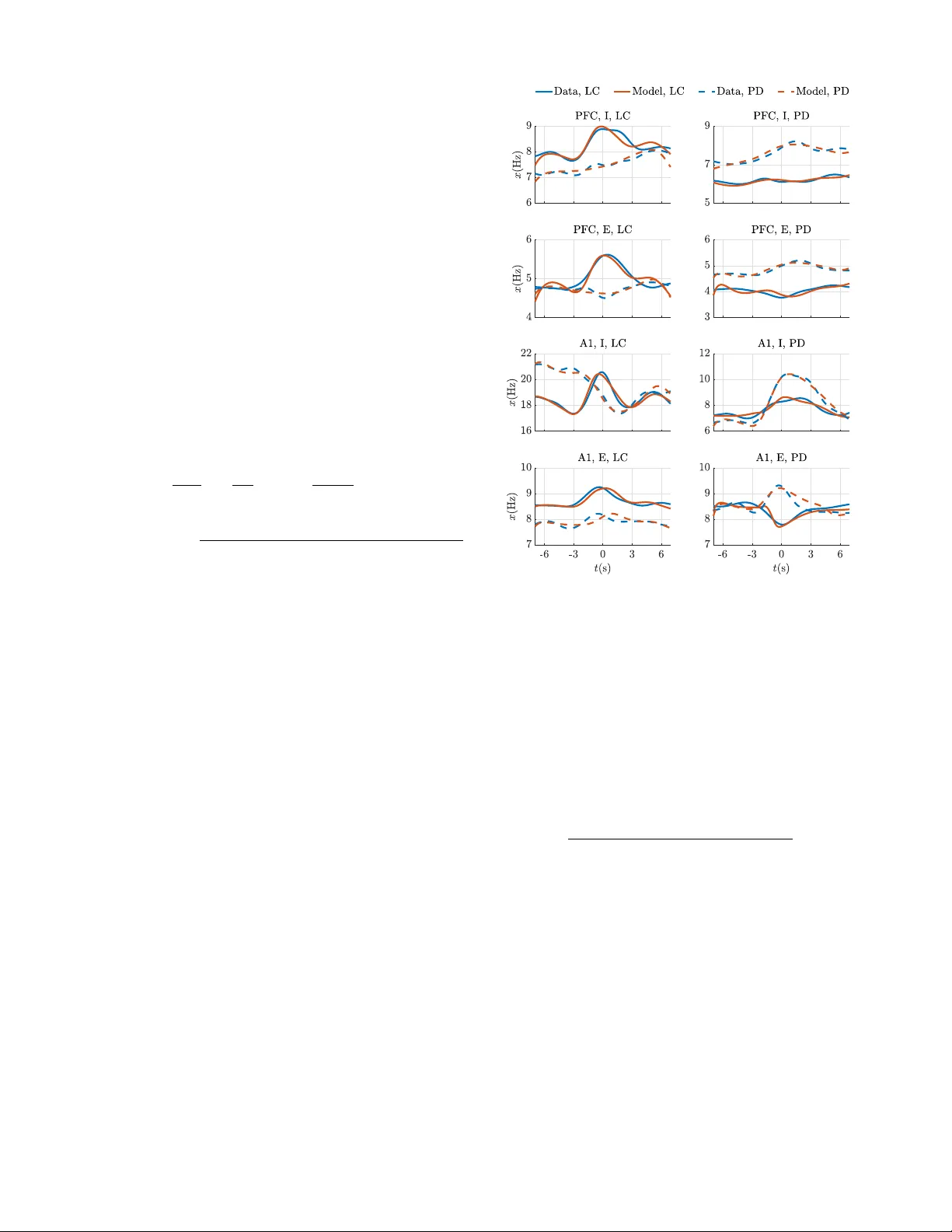
Hierar chical Selectiv e Recruitment in Linear -Thr eshold Brain Networks Part II: Multi-Lay er Dynamics and T op-Down Recruitment Erfan Nozari Jorge Cort ´ es Abstract —Goal-driven selective attention (GDSA) is a remark- able function that allows the complex dynamical networks of the brain to support coherent per ception and cognition. Part I of this two-part paper proposes a new control-theoretic framework, termed hierarchical selective recruitment (HSR), to rigorously explain the emergence of GDSA fr om the brain’ s network structure and dynamics. This part completes the development of HSR by deriving conditions on the joint structur e of the hierarchical subnetw orks that guarantee top-down r ecruitment of the task-rele vant part of each subnetwork by the subnetwork at the layer immediately above, while inhibiting the activity of task- irrele vant subnetw orks at all the hierar chical layers. T o further verify the merit and applicability of this framework, we carry out a compr ehensive case study of selective listening in rodents and show that a small network with HSR-based structure and minimal size can explain the data with r emarkable accuracy while satisfying the theoretical requirements of HSR. Our technical approach relies on the theory of switched systems and provides a novel converse L yapunov theorem for state-dependent switched affine systems that is of independent interest. I . I N T RO D U C T I O N Our ability to construct a dynamic yet coherent percep- tion of the world, despite the numerous parallel sources of information that affect our senses, is to a great extent reliant on the brain’ s capability to prioritize the processing of task- relev ant information over task-irrele vant distractions according to one’ s goals and desires. This capability , commonly known as goal-dri ven selecti ve attention (GDSA), has been the subject of extensiv e research o ver the past decades. Despite major advances, a fundamental understanding of GDSA and, in particular , how it emerges from the dynamics of the underlying neuronal networks, is still missing. The aim of this work is to reduce this gap by bringing tools and insights from systems and control theory into these questions from neuroscience. In this two-part paper, we propose the novel theoretical framew ork of Hierarchical Selectiv e Recruitment (HSR) for GDSA. As stated in Part I, HSR consists of a nov el hi- erarchical model of brain or ganization, a set of analytical results regarding the multi-timescale dynamics of this model, and a careful translation between the properties of these dynamics and well known experimental observ ations about GDSA. Inspired and supported by extensi ve experimental research [2]–[14], HSR relies on four major assumptions about the neuronal mechanisms underlying GDSA. These include (i) the brain’ s hierarchical organization, so that (cognitively- )higher areas provide control inputs to the activity of lower lev el ones [6], [8]–[10], [12]–[14], (ii) its sparse coding, so A preliminary version appeared as [1] at the IEEE Conference on Decision and Control Erfan Nozari is with the Department of Electrical and Systems Engineering, Univ ersity of Pennsylvania, enozari@seas.upenn.edu. Jorge Cort ´ es is with the Department of Mechanical and Aerospace Engineering, University of California, San Diego, cortes@ucsd.edu. that task-relev ant and task-irrelev ant stimuli is represented and processed by sufficiently distinct neuronal populations (particularly if the two stimuli differ in major or multiple properties, such as location, sensory modality , etc.) [4]–[9], [12], [14], (iii) the distributed and graded nature of GDSA, so that selectiv e attention happens at multiple layers of the hierarchy [3], [5]–[9], [11], [12], [14], and (i v) the concurrence of the suppression and enhancement of task-irrele v ant and task-relev ant activity , resp. [2]–[7], [9]–[14] (formulated as selective inhibition and top-down recruitment in HSR, resp.). The hierarchical structure of the brain plays a key role in both selective inhibition and top-down recruitment. The position of brain areas along this hierarchy is determined based on the direction in which sensory information and decisions flow , b ut also by the separation of timescales between the areas. As expected, the timescale of the internal dynamics of the neuronal populations increases (becomes slower) as one mov es up the hierarchy [15]–[21]. Although this hierarchy of timescales is well known in neuroscience, its role in GDSA has remained, to the best of our knowledge, uncharacterized. Using tools from singular perturbation theory , we here re veal the critical role played by this separation of timescales in the top-down recruitment of the task-relev ant subnetworks and provide rigorous conditions on the joint structure of all layers that guarantee such recruitment. Literatur e Review: The hierarchical organization of the brain has been recognized for decades [22]–[24] and applies to multiple aspects of brain structure and function. These aspects include (i) network topology [24]–[27] (where nodes are assigned to layers based on their position on bottom- up and top-do wn pathways), (ii) encoding properties [28], [29] (where nodes that hav e larger receptive fields and/or encode more abstract stimulus properties constitute higher layers), (iii) dynamical timescale [15]–[21], [25], [27], [30]– [34] (where nodes are grouped into layers according to the timescale of their dynamics), (iv) nodal clustering [35]–[38] (where nodes only constitute the leafs of a clustering tree), and (v) oscillatory activity [39] (where layers correspond to nested oscillatory frequency bands). Note that while hierarchical layers are composed of brain regions in (i)-(iii), this is not the case for (iv) and (v). The hierarchies (i)-(iii) are remarkably similar (in terms of the assignment of brain regions to the layers of the hierarchy), and here we particularly focus on (iii) (the timescale separation between hierarchical layers) as it plays a piv otal role in HSR. Studies of timescale separation between cortical regions are more recent. Se veral experimental works have demonstrated a clear increase in intrinsic timescales as one moves up the hierarchy using indirect measures such as the length of stim- ulus presentation that elicits a response [15], [16], resonance frequency [17], the length of the largest time window over which the responses to successive stimuli interfere [18], and how quickly the activ ation lev el of any brain region can track changes in sensory stimuli [19]. Direct e vidence for this hier- archical separation of timescales was indeed provided in [20] using the decay rate of spike-count autocorrelation functions. This was shown ev en more comprehensively in [21] using linear-threshold rate models and the concept of continuous hierar chies [25], [27] (whereby the layer of each node can vary continuously according to its intrinsic timescale, therefore removing the rigidity and arbitrariness of node assignment in classical hierarchical structures). Interestingly , recent studies show that this timescale variability may have roots not only in synaptic dynamics of individual neurons [30], but also in sub- neuronal genetic factors [31] as well as supra-neuronal net- work structures [32]. In terms of applications, computational models of motor control were perhaps the first to exploit this cortical hierarchy of timescales [33], [34]. Despite the vastness of the literature on its roots and applications, we are not aw are of any theoretical analysis of the effects of this separation of timescales on the hierarchical dynamics of neuronal networks. The accompan ying P art I [40] proposes the HSR frame work, which is strongly rooted in this separation of timescales. Part I analyzes the internal dynamics of the subnetworks at each layer of the hierarchy . Using the class of linear-threshold network models, it characterizes the networks that have a unique equilibrium, are locally/globally asymptotically stable, and have bounded trajectories. In Part I, we also provide a detailed account of feedforward and feedback mechanisms for selectiv e inhibition between any two layers of the hierarchy and show that the internal dynamical properties of the task- relev ant subnetwork at each layer is the sole determiner of the dynamical properties achiev able under selective inhibition. In this paper, we complete the development of the HSR framew ork for GDSA by analyzing the mechanisms for top- down recruitment of the task-relev ant subnetwork, combining it with the feedforward and feedback mechanisms of selectiv e inhibition, and generalizing the combination to arbitrary num- ber of layers. T op-down recruitment is one of the most exper - imentally well-documented phenomena in selectiv e attention, see, e.g., [4]–[9], [12]–[14]. While the enhancement (a.k.a. modulation ) of activity in the task-relev ant populations is the simplest form of recruitment, our model is general and thus also allows for more complex observed forms of recruitment, such as changes in the receptive fields 1 [41]–[43]. In the analysis of top-do wn recruitment, we use tools from singular perturbation theory to rigorously le verage this separation of timescales. The classical result on singularly perturbed ODEs goes back to T ikhonov [44], [45, Thm 11.1] and has since inspired an extensi ve literature, see, e.g. [46]– [49]. Tikhono v’ s result, howe ver , requires smoothness of the vector fields, which is not satisfied by linear-threshold dy- namics. Fortunately , sev eral works hav e sought extensions to non-smooth differential equations and ev en differential inclu- sions [50]–[53], culminating in the work [54] which we use here. Similar to T ikhonov’ s original work, [54] only applies to finite intervals. Extensions to infinite intervals exist [55], 1 The receptiv e field of each neuron is the area in the stimulus space where the neuron is responsiv e to the presence of stimuli. [56] but, as expected, they require asymptotic stability of the reduced-order model (ROM) which we do not in general ha ve. 2 Statement of Contributions: The paper has four main contri- butions. First, we use the timescale separation in hierarchical brain networks and the theory of singular perturbations to provide an analytic account of top-down recruitment in terms of conditions on the network structure. These conditions guarantee the stability of the task-rele vant part of a (fast) linear-threshold subnetwork to wards a reference trajectory set by a slower subnetwork. This, in particular, subsumes the most classical enhancement (strengthening) of the activity of task-relev ant nodes but is more general and can account for recent, complex observ ations such as changes in neuronal receptiv e fields under GDSA 1 . W e further combine these results with the results of Part I to allo w for simultaneous selectiv e inhibition and top-down recruitment, as observed in GDSA. Second, we extend this combination to hierarchical structures with an arbitrary number of layers, as observed in nature, to yield a fully dev eloped HSR framework. Here, we also deriv e an extension of the stability results in P art I that guarantees GES of a multi-layer multiple timescale linear-threshold network. Third, to validate the proposed HSR framew ork, we provide a detailed case study of GDSA in real brain networks. Using single-unit recordings from two brain regions of rodents performing a selectiv e listening task, we pro vide an in-depth analysis of appropriate choices of neuronal populations in each brain region as well as the timescales of their dynamics. W e propose a novel hierarchical structure for these populations, tune the parameters of the resulting network using a novel objectiv e function, and show that the resulting structure conforms to the theoretical results and requirements of HSR while explaining more than 90% of variability in the data. As part of our technical approach, our fourth and final contribution is a nov el con verse L yapunov theorem that extends the state of the art on GES for state- dependent switched affine systems. This result only requires continuity of the vector field and guarantees the existence of an infinitely smooth quadratically-growing L yapunov function if the dynamics is GES. Because of independent interest, we formulate and pro ve the result for general state-dependent switched affine systems. 3 I I . P RO B L E M S TA T E M E N T The problem formulation is the same as in Part I [40]. W e include here a streamlined description for a self-contained 2 Recall that in two-timescale dynamics, ROM results from replacing the fast variable with its equilibrium (reducing order to that of the slow variable). 3 Throughout the paper , we use the following notation. R , R ≥ 0 , R ≤ 0 , and R > 0 denote the set of reals, nonnegativ e reals, nonpositive reals, and positive reals, resp. 1 n , 0 n , 0 p × n , and I n stand for the n -vector of all ones, the n -vector of all zeros, the p -by- n zero matrix, and the identity n -by- n matrix, resp. The subscripts are omitted when clear from the context. When a vector x or matrix A are block-partitioned, x i and A ij refer to the i th block of x and ( i, j ) th block of A , resp. Given A ∈ R n × n , its element-wise absolute value and spectral radius are | A | and ρ ( A ) , resp. k · k denotes vector 2 -norm. For x ∈ R and m ∈ R > 0 ∪ {∞} , [ x ] m 0 = min { max { x, 0 } , m } , which is the projection of x onto [0 , m ] . When x ∈ R n and m ∈ R n > 0 ∪ {∞} n , we similarly define [ x ] m 0 = [[ x 1 ] m 1 0 · · · [ x n ] m n 0 ] T . For σ ∈ { 0 , `, s } n , Σ ` = Σ ` ( σ ) is a diagonal matrix with Σ ` ii = 1 if σ i = ` and Σ ` ii = 0 otherwise. Σ s is defined similarly . W e set the conv ention that Σ s m = 0 if Σ s = 0 and m = ∞ 1 n . For D ⊆ R n and A ∈ R p × n , b ∈ R p , we let A D + b = { Ax + b | x ∈ D } . . . . . . . Subnetwork i − 1 Subnetwork i Subnetwork i + 1 N 0 i (inhibited, state = x 0 i ) N 1 i (recruited, state = x 1 i ) Fig. 1: Hierarchical network structure considered in this work. exposition. W e consider a hierarchical neuronal network N , cf. Figure 1, whereby the nodes in each layer N i are further decomposed into a task-irrelev ant part N 0 i and a task-relev ant part N 1 i . The state evolution of each layer N i is modeled with linear-threshold network dynamics of the form τ i ˙ x i ( t ) = − x i ( t ) + [ W i,i x i ( t ) + d i ( t )] m i 0 , 0 ≤ x i (0) ≤ m i , m i ∈ R n > 0 ∪ {∞} n , (1) where x i ∈ R n i , W i,i ∈ R n i × n i , d i ∈ R n i , and m ∈ R n > 0 denote the state, internal synaptic connectivity , e xternal inputs, and state upper bounds of N i , resp. 4 The dev elopment of HSR is structured in four thrusts: (i) the analysis of the relationship between structure ( W i,i ) and dynamical behavior for each subnetwork when operating in isolation from the rest of the network ( d i ( t ) ≡ d i ); (ii) the analysis of the conditions on the joint structure of each two successive layers N i and N i +1 that allows for selectiv e inhibition of N 0 i +1 by its input from N i , being equiv alent to the stabilization of N 0 i +1 to the origin (inacti vity); (iii) the analysis of the conditions on the joint structure of each two successive layers N i and N i +1 that allows for top-down recruitment of N 1 i +1 by its input from N i , being equiv alent to the stabilization of N 1 i +1 tow ard a desired trajectory set by N i (activity); (iv) the combination of (ii) and (iii) in a unified framework and its extension to the complete N -layer network of networks. Problems (i) and (ii) are addressed in Part I [40], while problems (iii) and (iv) are the subject of this work. W e let d i ( t ) = B i u i ( t ) + ˜ d i ( t ) , u i ∈ R p i ≥ 0 , (2) where u i is the top-down control used for inhibition of N 0 i . While in Part I we assumed for simplicity that ˜ d i ( t ) is giv en and constant, we here consider its complete form ˜ d i ( t ) = W i,i − 1 x i − 1 ( t ) + W i,i +1 x i +1 ( t ) + c i , where the inter-layer connectivity matrices W i,i − 1 and W i,i +1 hav e appropriate dimensions and c i ∈ R n i captures 4 W e note that this is a standard and widely used model in computational neuroscience, as mentioned in Part I [40]. Please see therein for a detailed literature re view of its origins and prior analysis. un-modeled background activity and possibly nonzero activ a- tion thresholds. Substituting these into (1), the dynamics of each layer N i is giv en by τ i ˙ x i ( t ) = − x i ( t ) + [ W i,i x i ( t ) + W i,i − 1 x i − 1 ( t ) (3) + W i,i +1 x i +1 ( t ) + B i u i ( t ) + c i ] m i 0 . Also following Part I, we partition network variables as x i = " x 0 i x 1 i # , W i,j = " W 00 i,j W 01 i,j W 10 i,j W 11 i,j # , B i = " B 0 i 0 # , c i = " c 0 i c 1 i # , m i = " m 0 i m 1 i , # (4) where x 0 i ∈ R r i for all i, j ∈ { 1 , . . . , N } . By con vention, W 1 , 0 = 0 , W N ,N +1 = 0 , and r 1 = 0 (so B 1 = 0 and the first subnetwork has no inhibited part). W e assume that the hierarchical layers hav e suf ficient timescale separation, i.e., τ 1  τ 2  · · ·  τ N . (5) Finally , let  = (  1 , . . . ,  N − 1 ) , with  i = τ i +1 /τ i , i = { 1 , . . . , N − 1 } . (6) Next, we first dev elop the main concepts and results for the case of bilayer networks (Section III) and then extend them to the setup with N layers (Section IV). I I I . S E L E C T I V E R E C RU I T M E N T I N B I L A Y E R N E T W O R K S In this section we tackle the analysis of simultaneous selectiv e inhibition and top-do wn recruitment in a two-layer network. W e consider the same dynamics as in (3) for the lower -lev el subnetwork N 2 , but temporarily allo w the dy- namics of N 1 to be arbitrary . This setup allo ws us to study the key ingredients of selectiv e recruitment without the extra complications that arise from the multilayer interconnections of linear-threshold subnetworks and is the basis for our later dev elopments. Further, by keeping the higher-le vel dynamics arbitrary , the results presented here are also of independent interest beyond HSR, as they allo w for a broader range of external inputs d ( t ) than those generated by linear-threshold dynamics. This can be of interest in, for example, direct brain stimulation applications where x 1 ( t ) is generated and applied by a computer in order to control the activity x 2 ( t ) of certain areas of the brain. In this view , appropriate stimulation signals x 1 ( t ) may be considered as an augmentation of the natural hierarchy of the brain if they v ary slow enough to satisfy (5). Section IV builds on the insights obtained here to generalize this framework to the multilayer case described in Section II. For any W ∈ R n × n , define h : R n ⇒ R n ≥ 0 by h ( d ) = h W , m ( d ) , { x ∈ R n ≥ 0 | x = [ Wx + d ] m 0 } , (7) which maps any constant input d ∈ R n to the corresponding set of the equilibria of (1). Due to the switched-affine form of the dynamics, h has the piecewise-af fine form h ( d ) = { F σ d + f σ | G σ d + g σ ≥ 0 , σ ∈ { 0 , `, s } n } , (8) F σ = ( I − Σ ` W ) − 1 Σ ` , f σ = ( I − Σ ` W ) − 1 Σ s m , G σ =  Σ ` + Σ s − I Σ ` − Σ ` Σ s  T F σ , g σ =  f T σ ( Σ ` + Σ s − I ) f T σ Σ ` ( m − f σ ) T Σ ` ( f σ − m ) T Σ s  T . The existence and uniqueness of equilibria of (1) precisely corresponds to h being single-v alued on R n , in which case we let h : R n → R n ≥ 0 be an ordinary function. For our subsequent analysis we need h to be Lipschitz, as stated next. The proof of this result is a special case of Lemma IV .2 and thus omitted. Lemma III.1. (Lipschitzness of h ). Let h be as in (7) and single-valued 5 on R n . Then, it is globally Lipschitz on R n . The main result of this section is as follo ws. Theorem III.2. (Selective recruitment in bilayer networks). Consider the multilayer dynamics (3) where N = 2 , W 01 2 , 1 = 0 , and c 0 2 = 0 but x 1 ( t ) is generated by the dynamics τ 1 ˙ x 1 ( t ) = γ ( x 1 ( t ) , x 2 ( t ) , t ) . (9) Let h 1 2 = h W 11 2 , 2 , m 1 2 as in (7) . If (i) γ is measurable in t , locally bounded, and locally Lips- chitz in ( x 1 , x 2 ) uniformly in t ; (ii) (9) has bounded solutions uniformly in x 2 ( t ) ; (iii) p 2 ≥ r 2 ; (iv) W 11 2 , 2 is such that τ ˙ x 1 2 = − x 1 2 + [ W 11 2 , 2 x 1 2 + d 1 1 ] m 1 2 0 is GES towar ds a unique equilibrium for any constant d 1 1 ; then there e xists K 2 ∈ R p 2 × n 2 such that by using the feedback contr ol u 2 ( t ) = K 2 x 2 ( t ) , one has lim  1 → 0 sup t ∈ [ t, ¯ t ]    x 2 ( t ) −  0 r 2 , h 1 2  W 11 21 x 1 ( t ) + c 1 2      = 0 , (10) for any 0 < t < ¯ t < ∞ , with  1 given in (6) . Further , if the dynamics of x 2 is monotonically bounded 6 , ther e also exists a feedforwar d contr ol u 2 ( t ) ≡ ¯ u 2 such that (10) holds for any 0 < t < ¯ t < ∞ and arbitrary W 01 2 , 1 and c 0 2 . Pr oof: First we prove the result for feedback control. By (iii) , there exists K 2 ∈ R p 2 × n 2 almost always (i.e., for almost all ( W 00 2 , 2 , W 01 2 , 2 , B 0 2 ) ) such that W 2 , 2 + B 2 K 2 =  0 0 W 10 2 , 2 W 11 2 , 2  . (11) Further , by [40, Thm IV .7(ii) & Thm V .3(ii)], all the principal submatrices of − I + ( W 2 , 2 + B 2 K 2 ) are Hurwitz. Therefore, by [40, Thm IV .3 & Assump. 1], h 1 2 is singleton-valued almost always (i.e., for almost all W 2 , 2 ). Thus, the x 2 -dynamics is τ 2 ˙ x 0 2 = − x 0 2 , (12) τ 2 ˙ x 1 2 = − x 1 2 + [ W 10 2 , 2 x 0 2 + W 11 2 , 2 x 1 2 + W 11 2 , 1 x 1 + c 1 2 ] m 1 2 0 , and has a unique equilibrium for an y fixed x 1 . Assumption (iv) and [40, Lemma A.2] then ensure that (12) is GES relative to ( 0 r 2 , h 1 2 ( W 11 21 x 1 ( t ) + c 1 2 )) for any fixed x 1 . Based on assumption (ii) , let D ⊂ R n be a compact set that contains the trajectory of the reduced-order model τ 1 ˙ x 1 = γ ( x 1 , ( 0 r 2 , h 1 2 ( W 11 21 x 1 ( t ) + c 1 2 )) , t ) . By assumption (i) , γ is Lipschitz in ( x 1 , x 2 ) on compacts uniformly in t . Let L γ be its 5 It is possible to show , using the same proof technique, that h is Lipschitz in the Hausdorff metric even when it is multiple-valued (recall that the Hausdorff distance between two sets S 1 , S 2 ∈ R n is defined as max { sup a ∈ S 1 inf b ∈ S 2 k a − b k , sup b ∈ S 2 inf a ∈ S 1 k a − b k} ). 6 See [40, Def V .1]. associated Lipschitz constant on D × { 0 r 2 } × h 1 2 ( W 11 2 , 1 D + c 1 2 ) . Using (8) and Lemma III.1, for all x 1 , ˆ x 1 ∈ D , k γ ( x 1 , h 1 2 ( W 11 2 , 1 x 1 + c 1 2 ) , t ) − γ ( ˆ x 1 , h 1 2 ( W 11 2 , 1 ˆ x 1 + c 1 2 ) , t ) k ≤ L γ k ( x 1 − ˆ x 1 , h 1 2 ( W 11 2 , 1 x 1 + c 1 2 ) − h 1 2 ( W 11 2 , 1 ˆ x 1 + c 1 2 )) k ≤ L γ ( k x 1 − ˆ x 1 k + k h 1 2 ( W 11 2 , 1 x 1 + c 1 2 ) − h 1 2 ( W 11 2 , 1 ˆ x 1 + c 1 2 ) k ) ≤ L γ (1 + L h k W 11 2 , 1 k ) k x 1 − ˆ x 1 k , so γ ( · , h 1 2 ( W 11 2 , 1 · + c 1 2 ) , t ) : R n 1 → R n 1 is L γ (1 + L h k W 11 2 , 1 k ) - Lipschitz on D . Using this, Lemma IV .2 again, and the change of variables t 0 , t/τ 1 , the claim follows from [54, Prop 1]. 7 Next, we prov e the result for constant feedforward control u 2 ( t ) ≡ ¯ u 2 . Based on assumption (ii) , let ¯ x 1 ∈ R n 1 > 0 be the bound on the trajectories of (9) and ¯ u 2 be a solution of B 0 2 ¯ u 2 = − [[ W 00 2 , 2 W 01 2 , 2 ]] ∞ 0 ν ( ¯ x 1 ) − [ W 01 2 , 1 ] ∞ 0 ¯ x 1 + [ c 0 2 ] ∞ 0 , where ν comes from the monotone boundedness of the dynamics of x 2 . This solution almost alw ays exists by as- sumption (ii) . Then, the dynamics of x 2 simplifies to (12), and [40, Lemma A.2] guarantees that it is GES relati ve to ( 0 r 2 , h 1 2 ( W 11 2 , 1 x 1 + c 1 2 )) for an y fixed x 1 . The claim then follows, similar to the feedback case, from [54, Prop 1]. Remark III.3. (V alidity of the assumptions of Theo- rem III.2.). Assumption (i) is merely technical and satisfied by all well-known models of neuronal rate dynamics, including the linear-threshold model itself. Likewise, assumption (ii) is always satisfied in reality , as the firing rates of all biological neuronal networks are bounded by the inv erse of the refrac- tory period of their neurons. In theory , the verification of this assumption depends clearly on γ . If a linear-threshold model is used, we can instead use Theorem IV .3 and relax assumption (ii) to a less restricti ve one (assumption (i) of Theorem IV .3), which can in turn be verified using the sufficient condition in Theorem IV .4. Assumption (iii) requires the existence of at least as many inhibitory control channels as the number of nodes in N 2 that are to be inhibited. Indeed, selectiv e inhibition is still possible without this assumption (cf. Theorem IV .3), but may require excessi ve inhibitory resources. The most critical requirement is assumption (iv) , but is not only sufficient but also necessary for inhibitory stabilization (cf. [40, Thm IV .8] for conditions on W 11 2 , 2 that ensure this assumption as well as [40, Thm V .2 & V .3] for its necessity for feedforward and feedback inhibitory stabilization) .  The main conclusion of Theorem III.2 is the T ikhonov- type singular perturbation statement in (10). According to this statement, the tracking error can be made arbitrarily small, i.e., for any θ > 0 , | x 2 ( t ) − ( 0 r 2 , h 1 2 ( x 1 ( t ))) | ≤ θ 1 n 2 , ∀ t ∈ [ t, ¯ t ] , (13) provided that τ 2 /τ 1 is sufficiently small. As discussed in Sec- tion I, this timescale separation is characteristic of biological 7 [54, Prop 1] is applicable to singularly perturbed differential inclusions and thus technically inv olved, but for non-smooth ODEs such as (3), its assumptions can be simplified to: 1. Lipschitzness of dynamics uniformly in t , 2. Existence, uniqueness, and Lipschitzness of the equilibrium map of fast dynamics, 3. Lipschitzness and boundedness of the reduced-order model, 4. asymptotic stability of the fast dynamics uniformly in t and the slow variable, and 5. global attractivity of fast dynamics for any fixed slow variable. Inhibitory τ 1 Excitatory τ 2 = 0 . 5 τ 1 Fig. 2: The network structure (right) and trajectories (left) of the tw o-timescale network in (14) for τ 1 = 3 . 3 ms . The red pyramids and blue circles depict excitatory and inhibitory nodes, resp., and the trajectory colors on the left correspond to node colors on the right. The dashed lines show the desired reference trajectories  0 , h 1 2 ( W 11 2 , 1 x 1 ( t ) + c 1 2 )  . neuronal networks. In general, the smaller the time constant ratio τ 2 /τ 1 , the smaller the tracking error θ . As sho wn in [20], sev eral pairs of regions along the sensory-frontal pathways hav e successiv e time constant ratios between 1 / 1 . 5 and 1 / 2 . 5 , which is often (more than) enough in simulations for (13) to hold with small enough θ , as sho wn in Example III.4 below . An important observation regarding (13) is that the equi- librium map h 1 2 does not have a closed-form expression, so the reference trajectory h 1 2 ( x 1 ( t )) of the lower -lev el network is only implicitly known for an y gi ven x 1 ( t ) . Ho wever , if a desired trajectory ξ 1 2 ( t ) ∈ Q n 2 j = r 2 +1 [0 , m 2 ,j ] for x 1 2 is known a priori, one can specify the appropriate γ such that h 1 2 ( x 1 ( t )) = ξ 1 2 ( t ) . T o show this, let the dynamics of ξ 1 2 ( t ) be τ 1 ˙ ξ 1 2 ( t ) = γ ξ ( ξ 1 2 ( t ) , t ) . Then, choosing x 1 ( t ) = ( W 11 2 , 1 ) − 1  ( I − W 11 2 , 2 ) ξ 1 2 ( t ) − c 1 2  , [ W 11 2 , 2 ξ 1 2 ( t ) + W 11 2 , 1 x 1 ( t ) + c 1 2 ] m 1 2 0 = [ ξ 1 2 ( t )] m 1 2 0 = ξ 1 2 ( t ) , which, according to (7), implies ξ 1 2 ( t ) = h 1 2 ( x 1 ( t )) . W e use this result to illustrate the core concepts of the bilayer HSR in a synthetic but biologically-inspired example, where a inhibitory subnetwork generates oscillations which are selectiv ely induced on a lower -lev el excitatory subnetwork. Example III.4. (HSR of an excitatory subnetwork by in- hibitory oscillations). Consider the dynamics (3) with N = 2 , a 3 -dimensional excitatory subnetwork at the lower lev el, a 3 -dimensional inhibitory subnetwork at the higher lev el, and m 1 = m 2 = ∞ 1 3 (Figure 2). Let W 1 , 1 =   0 − 0 . 8 − 1 . 7 − 1 0 − 0 . 5 − 0 . 7 − 1 . 8 0   , c 1 =   11 10 10   , W 2 , 2 =   0 0 . 9 1 . 2 0 . 7 0 1 0 . 8 0 . 2 0   , B 2 =   − 1 0 0   , c 2 =   2 3 . 5 2 . 5   , W 1 , 2 = 0 , W 2 , 1 = − I , u 2 = 5 . (14) This example satisfies all the assumptions of Theorem III.2, so we expect the actual x 2 -trajectory to be close to the desir ed x 2 -trajectory (0 , h 1 2 ( x 1 ( t )) provided that  1  1 . As shown in Figure 2, x 2 ( t ) and (0 , h 1 2 ( x 1 ( t )) are remarkably close e ven with a mild separation of timescales,  1 = 0 . 5 . This example further illustrates the complementary roles of selectiv e inhibition and selectiv e recruitment. The complete x 2 -subsystem is unstable by itself, but any two-dimensional subnetwork of it is stable. Therefore, N 1 can selecti vely inhibit any single node of N 2 while simultaneously recruiting (e.g., by inducing oscillations in) the remaining two. Thus, as suggested earlier in [40, Rem V .7], different “tasks” can be accomplished at different times by varying the selectively recruited subnet- work ov er time. Generalizing this to more complex networks allows for more flexible selective recruitment schemes of larger neuronal subnetworks, as observed in nature.  Remark III.5. (Biological relevance of Example III.4). In addition to providing a simple illustration of the HSR framew ork dev eloped here, Example III.4 has interesting sim- ilarities with well-kno wn aspects of selecti ve attention in the brain. Extensi ve studies hav e demonstrated a robust correlation between oscillatory acti vity , particularly in the gamma range ( ∼ 30 − 100 Hz ), and selectiv e attention [57]–[60]. Furthermore, gamma oscillations in the cortex are shown to be primarily generated by networks of inhibitory neurons, which then recruit the excitatory populations (see [61] and the references therein), as captured by the network structure of Figure 2. Interestingly , the oscillations generated by the higher-lev el inhibitory subnetwork fall within the gamma band by setting τ 1 ∼ 3 ms which lies within the decay time constant range of GAB A A inhibitory receptors 8 (the major type of inhibitory synapse in the central nervous system).  I V . S E L E C T I V E R E C RU I T M E N T I N M U LT I LAY E R N E T WO R K S W e tackle here the problem of Section II in its general form and consider an N -layer hierarchical structure of subnetworks with linear-threshold dynamics. Given (3), let h 1 i : c 1 i ⇒ { x 1 i | x 1 i = [ W 11 i,i +1 h 1 i +1 ( W 11 i +1 ,i x 1 i + c 1 i +1 ) + W 11 i,i x 1 i + c 1 i ] m 1 i 0 } , i = 2 , . . . , N − 1 , with h 1 N = h W 11 N,N , m 1 N , be the recursive definition of the (set-valued) equilibrium maps of the task-relev ant parts of the layers { 2 , . . . , N } . These maps play a central role in the multiple-timescale dynamics of (3). Therefore, we begin by characterizing their piecewise-af fine nature. The proof of the following result can be found in Appendix B. Lemma IV .1. (Piecewise affinity of equilibrium maps is preserved along layers of hierarchical linear-threshold net- work). Let h : R n → R n be a piecewise affine function, h ( c ) = F λ c + f λ , ∀ c ∈ Ψ λ , { c | G λ c + g λ ≥ 0 } , ∀ λ ∈ Λ , wher e Λ is a finite index set and S λ ∈ Λ Ψ λ = R n . Given matrices W ` , ` = 1 , 2 , 3 and a vector ¯ c , assume x = [ W 1 x + W 2 h ( W 3 x + ¯ c ) + c 0 ] m 0 , (15) 8 See, e.g., the Neurotransmitter Time Constants database of the CNR- Glab at the University of W aterloo, http://compneuro.uwaterloo.ca/research/ constants- constraints/neurotransmitter- time- constants- pscs.html. is known to have a unique solution x ∈ R n 0 for all c 0 ∈ R n 0 and let h 0 ( c 0 ) be this unique solution. Then, there exists a finite index set Λ 0 and { ( F 0 λ 0 , f 0 λ 0 , G 0 λ 0 , g 0 λ 0 ) } λ 0 ∈ Λ 0 such that h 0 ( c 0 ) = F 0 λ 0 c 0 + f 0 λ 0 , ∀ c 0 ∈ Ψ 0 λ 0 , { c 0 | G 0 λ 0 c 0 + g 0 λ 0 ≥ 0 } , ∀ λ 0 ∈ Λ 0 , (16) and S λ 0 ∈ Λ 0 Ψ 0 λ 0 = R n 0 .  A special case of Lemma IV .1 is when W 2 = 0 , where h 0 becomes, like h 1 N , the standard equilibrium map (7). Next, we characterize the global Lipschitzness property of the equilibrium maps. The proof is in Appendix B. Lemma IV .2. (Piecewise affine equilibrium maps are glob- ally Lipschitz). Let h : R n → R n be a piecewise affine function of the form h ( c ) = F λ c + f λ , ∀ c ∈ Ψ λ , { c | G λ c + g λ ≥ 0 } , ∀ λ ∈ Λ , wher e Λ is a finite index set and S λ ∈ Λ Ψ λ = R n . Then, h is globally Lipschitz.  W e are now ready to generalize Theorem III.2 to an N - layer architecture while at the same time relaxing se veral of its simplifying assumptions in fav or of generality . Theorem IV .3. (Selective recruitment in multilayer net- works). Consider the dynamics (3) . If (i) The reduced-or der model (R OM) τ 1 ˙ ¯ x 1 1 = − ¯ x 1 1 + [ W 11 1 , 1 ¯ x 1 1 + W 11 1 , 2 h 1 2 ( W 11 2 , 1 ¯ x 1 1 + c 1 2 ) + c 1 1 ] m 1 1 0 , of the first subnetwork has bounded solutions (r ecall x 1 ≡ x 1 1 since r 1 = 0 ); (ii) F or all i = 2 , . . . , N , τ i ˙ x 1 i ( t ) = − x 1 i ( t ) + [ W 11 i,i x 1 i ( t ) + W 11 i,i +1 h 1 i +1 ( W 11 i +1 ,i x 1 i ( t ) + c 1 i +1 ) + c 1 i ] m 1 i 0 , is GES towar ds a unique equilibrium for any c 1 i +1 and c 1 i ; then there exists K i ∈ R p i × n i and ¯ u i : R ≥ 0 → R p i ≥ 0 , i ∈ { 2 , . . . , N } such that using the feedback-feedforwar d contr ol u i ( t ) = K i x i ( t ) + ¯ u i ( t ) , i ∈ { 2 , . . . , N } , (17) we have, for any 0 < t < ¯ t < ∞ , lim  → 0 sup t ∈ [ t, ¯ t ] k x 0 i ( t ) k = 0 , ∀ i ∈ { 2 , . . . , N } , (18a) and lim  → 0 sup t ∈ [0 , ¯ t ] k x 1 1 ( t ) − ¯ x 1 1 ( t ) k = 0 , (18b) lim  → 0 sup t ∈ [ t, ¯ t ] k x 1 2 ( t ) − h 1 2 ( W 11 2 , 1 x 1 1 ( t ) + c 1 2 ) k = 0 , (18c) . . . lim  → 0 sup t ∈ [ t, ¯ t ] k x 1 N ( t ) − h 1 N ( W 11 N ,N − 1 x 1 N − 1 ( t ) + c 1 N ) k = 0 . (18d) Pr oof: For any 2 × 2 block-partitioned matrix W , we introduce the con venient notation W `, all , [ W ` 0 W ` 1 ] and W all ,` , [( W 0 ` ) T ( W 1 ` ) T ] T for ` = 0 , 1 . Further, for any i ∈ { 2 , . . . , N } , let x 1: i = [ x T 1 . . . x T i ] T . T o begin with, let K N and ¯ u N be such that B 0 N K N ≤ − W 0 , all N ,N , (19a) ¯ u N ( t ) ≤ − W 0 , all N ,N − 1 x N − 1 ( t ) − c 0 N , ∀ t, (19b) Note that, if p N ≥ r N , then (19a) can be satisfied with equality . Otherwise, (19a) can still be satisfied since all the rows of B 0 N are nonzero, but may require excessiv e amounts of inhibition. Also, notice that ¯ u N is set by the subnetwork N − 1 , which has access to x N − 1 ( t ) and can thus fulfill (19b). As a result, the nodes in x 0 N are fully inhibited and ev olve according to τ N ˙ x 0 N = − x 0 N . The overall dynamics become τ 1 ˙ x 1 = − x 1 + [ W 1 , 1 x 1 + W 1 , 2 x 2 + c 1 ] m 1 0 , . . . τ N − 1 ˙ x N − 1 = − x N − 1 + [ W N − 1 ,N − 1 x N − 1 + B N − 1 u N − 1 + W N − 1 ,N x N + W N − 1 ,N − 2 x N − 2 + c N − 1 ] m N − 1 0 ,  N − 1 τ N − 1 ˙ x 0 N = − x 0 N ,  N − 1 τ N − 1 ˙ x 1 N = − x 1 N + [ W 1 , all N ,N x N + W 1 , all N ,N − 1 x N − 1 + c 1 N ] m 1 N 0 . Letting  N − 1 → 0 , we get our first separation of timescales be- tween x N and x 1: N − 1 , as follo ws. For any constant x N − 1 , the x N dynamics is GES by assumption (ii) and [40, Lemma A.2]. Further , the equilibrium map h N = ( 0 r N , h 1 N ) of the N ’th subnetwork is globally Lipschitz by Lemmas IV .1 and IV .2, and the entire vector field of network dynamics is globally Lipschitz due to the Lipschitzness of [ · ] m 0 . Therefore, it follows from [54, Prop 1] that for any 0 < t < ¯ t < ∞ , lim  N − 1 → 0 sup t ∈ [ t, ¯ t ] k x 0 N ( t ) k = 0 , lim  N − 1 → 0 sup t ∈ [ t, ¯ t ] k x 1 N ( t ) − h 1 N ( W 1 , all N ,N − 1 x N − 1 ( t ) + c 1 N ) k = 0 , lim  N − 1 → 0 sup t ∈ [0 , ¯ t ] k x 1: N − 1 ( t ) − x (1) 1: N − 1 ( t ) k = 0 . Here, x (1) 1: N − 1 is the solution of the “first-step ROM” τ 1 ˙ x (1) 1 = − x (1) 1 + [ W 1 , 1 x (1) 1 + W 1 , 2 x (1) 2 + c 1 ] m 1 0 , . . . τ N − 1 ˙ x (1) N − 1 = − x (1) N − 1 + [ W N − 1 ,N − 1 x (1) N − 1 + W all , 1 N − 1 ,N h 1 N ( W 1 , all N ,N − 1 x (1) N − 1 ( t ) + c 1 N ) + W N − 1 ,N − 2 x (1) N − 2 + B N − 1 u N − 1 + c N − 1 ] m N − 1 0 , which results from replacing x N with its equilibrium value. Except for technical adjustments, the remainder of the proof essentially follows by repeating this process N − 2 times. In particular , for i = N − 1 , . . . , 2 , let K i and ¯ u i be such that B 0 i K i ≤ −| W 0 , all i,i | − | W 01 i,i +1 | ¯ F i +1 | W 1 , all i +1 ,i | , ¯ u i ( t ) ≤ − W 0 : i,i − 1 x i − 1 ( t ) − c 0 i , ∀ t, where ¯ F i ∈ R ( n i − r i ) × ( n i − r i ) is the entry-wise maximal gain of the map h 1 i ov er R n i − r i (cf. Theorem IV .4). This results in the “ ( N − i ) ’th-step R OM” τ 1 ˙ x ( N − i ) 1 = − x ( N − i ) 1 + [ W 1 , 1 x ( N − i ) 1 + W 1 , 2 x ( N − i ) 2 + c 1 ] m 1 0 , . . . τ i − 1 ˙ x ( N − i ) i − 1 = − x ( N − i ) i − 1 + [ W i − 1 ,i − 1 x ( N − i ) i − 1 + W i − 1 ,i x ( N − i ) i + W i − 1 ,i − 2 x ( N − i ) i − 2 + B i − 1 u i − 1 + c i − 1 ] m i − 1 0 ,  i − 1 τ i − 1 ˙ x ( N − i ) 0 i = − x ( N − i ) 0 i ,  i − 1 τ i − 1 ˙ x ( N − i ) 1 i = − x ( N − i ) 1 i + [ W 1 , all i,i x ( N − i ) 1 i + W all , 1 i,i +1 h 1 i +1 ( W 1 , all i +1 ,i x ( N − i ) i ( t ) + c 1 i +1 ) + W 1 , all i,i − 1 x ( N − i ) i − 1 + c 1 i ] m 1 i 0 . Similarly to above, in voking [54, Prop 1] then ensures that lim  → 0 sup t ∈ [ t, ¯ t ] k x ( N − i ) 0 i ( t ) k = 0 , lim  → 0 sup t ∈ [ t, ¯ t ] k x ( N − i ) 1 i ( t ) − h 1 i ( W 1 , all i,i − 1 x ( N − i ) i − 1 ( t ) + c 1 i ) k = 0 , lim  → 0 sup t ∈ [0 , ¯ t ] k x ( N − i ) 1: i − 1 ( t ) − x ( N − i +1) 1: i − 1 ( t ) k = 0 . Note that, after e very in vocation of [54, Prop 1], the super- index inside the parenthesis increases by 1 , showing one more replacement of a fast dynamics by its equilibrium state. In particular , after the ( N − 1) ’th in vocation of [54, Prop 1], we reach x ( N − 1) 1 1 , which is the same as ¯ x 1 1 in the statement. T ogether , these results (and sufficiently many applications of the triangle inequality and Lemma IV .2) ensure (18). An instructi ve difference, by design, between Theo- rems III.2 and IV .3 is the separate treatment of feedforward and feedback inhibition in the former versus the combina- tion of the two in the latter . While the separate treatment in Theorem III.2 is conceptually simpler and highlights the theoretical difference between the two inhibitory mechanisms, the combination in Theorem IV .3 results in more flexibility and less conservati veness: in pure feedforward inhibition, countering local excitations requires monotone boundedness and a suf ficiently large ¯ u providing inhibition under the worst- case scenario, a goal that is achiev ed more efficiently using feedback. On the other hand, pure feedback inhibition needs to dynamically cancel local excitations at all times and is also unable to counter the ef fects of constant background excitation, limitations that are easily addressed when combined with feedforward inhibition. Similar to Theorem III.2 (cf. Remark III.3), assumption (ii) of Theorem IV .3 is its only critical requirement which we next relate to the joint structure of the subnetworks. Theorem IV .4. (Sufficient condition for existence and uniqueness of equilibria and GES in multilayer linear- threshold networks). Let h : R n → R n be a piecewise affine function of the form h ( c ) = F λ c + f λ , ∀ c ∈ Ψ λ , { c | G λ c + g λ ≥ 0 } , ∀ λ ∈ Λ , (20) wher e Λ is a finite index set and S λ ∈ Λ Ψ λ = R n . Further , let ¯ F , max λ ∈ Λ | F λ | be the matrix whose elements are the maxi- mum of the corresponding elements fr om {| F λ |} λ ∈ Λ . F or arbi- trary matrices W ` , ` = 1 , 2 , 3 , if ρ  | W 1 | + | W 2 | ¯ F | W 3 |  < 1 , then the linear-thr eshold dynamics τ ˙ x ( t ) = − x ( t ) + [ W 1 x ( t ) + W 2 h ( W 3 x ( t ) + ¯ c ) + c ] m 0 , is GES towar ds a unique equilibrium for all ¯ c and c . Pr oof: W e use the same proof technique as in [62, Prop. 3]. For simplicity , assume that | W 1 | + | W 2 | ¯ F | W 3 | is irreducible (i.e., the network topology induced by it is strongly connected) 9 . Then, the left Perron-Frobenius eigenv ector α of | W 1 | + | W 2 | ¯ F | W 3 | has positiv e entries [63, Fact 4.11.4], making the map k · k α : v → k v k α , α T | v | a norm on R n . Further , it can be shown, similar to the proof of Lemma IV .2, that for all c 1 , c 2 ∈ R n , | h ( c 1 ) − h ( c 2 ) | ≤ ¯ F | c 1 − c 2 | , where the inequality is entrywise. Thus, for any x , ˆ x ∈ R n ,   [ W 1 x + W 2 h ( W 3 x + w ) + c ] m 0 − [ W 1 ˆ x + W 2 h ( W 3 ˆ x + w ) + c ] m 0   α = α T   [ W 1 x + W 2 h ( W 3 x + w ) + c ] m 0 − [ W 1 ˆ x + W 2 h ( W 3 ˆ x + w ) + c ] m 0   ≤ α T   W 1 ( x − ˆ x ) + W 2 ( h ( W 3 x + w ) − h ( W 3 ˆ x + w ))   ≤ α T  | W 1 | + | W 2 | ¯ F | W 3 |  | x − ˆ x | = ρ  | W 1 | + | W 2 | ¯ F | W 3 |  α T | x − ˆ x | = ρ  | W 1 | + | W 2 | ¯ F | W 3 |  k x − ˆ x k α . This proves that x 7→ [ W 1 x + W 2 h ( W 3 x + w ) + c ] m 0 is a contraction (on R n ≥ 0 if m = ∞ 1 n or on Q i [0 , m i ] if m < ∞ 1 n ) and has a unique fixed point, denoted x ∗ , by the Banach Fixed-Point Theorem [64, Thm 9.23]. T o show GES, let ξ ( t ) , ( x ( t ) − x ∗ ) e t , satisfying τ ˙ ξ ( t ) = M ( t ) W ξ ( t ) , (21) where M ( t ) is a diagonal matrix with diagonal entries M ii ( t ) ,  [ W 1 x ( t ) + W 2 h ( W 3 x ( t ) + w ) + c ] m 0 − x ∗ ) i ξ i ( t ) if ξ i ( t ) 6 = 0 and M ii ( t ) , 0 otherwise. Then | M ( t ) | ≤ | W 1 | + | W 2 | ¯ F | W 3 | , ∀ t ≥ 0 , where the inequality is entry-wise. Then, by using [65, Lemma] (which is essentially a careful application of Gronwall-Bellman’ s Inequality [45, Lemma A.1] to (21)), k ξ ( t ) k α ≤ k ξ (0) k α e ρ ( | W 1 | + | W 2 | ¯ F | W 3 | ) t ⇒ k x ( t ) − x ∗ k α ≤ k x (0) − x ∗ k α e − (1 − ρ ( | W 1 | + | W 2 | ¯ F | W 3 | )) t , establishing GES by the equiv alence of norms on R n . 9 If | W 1 | + | W 2 | ¯ F | W 3 | is not irreducible, it can be “upper-bounded” by the irreducible matrix | W 1 | + | W 2 | ¯ F | W 3 | + µ 1 n 1 T n , with µ > 0 sufficiently small such that ρ ( | W 1 | + | W 2 | ¯ F | W 3 | + µ 1 n 1 T n ) < 1 . The same argument can then be employed for this upper bound. Note that Theorem IV .4 applies to each layer of (3) sepa- rately . When put together , Theorem IV .3 (ii) is satisfied if ρ  | W 11 2 , 2 | + | W 11 2 , 3 | ¯ F 1 3 | W 11 3 , 2 |  < 1 , . . . ρ  | W 11 N − 1 ,N − 1 | + | W 11 N − 1 ,N | ¯ F 1 N | W 11 N ,N − 1 |  < 1 , ρ  | W 11 N ,N |  < 1 , (22) where ¯ F 1 i , i = 2 , . . . , N is the matrix described in Theo- rem IV .4 corresponding to h 1 i , and the af fine form (20) of h 1 i is computed recursiv ely using Lemma IV .1. Moreov er, if m 1 1 = ∞ 1 r 1 , then ρ  | W 11 1 , 1 | + | W 11 1 , 2 | ¯ F 1 2 | W 11 2 , 1 |  < 1 serves as a sufficient condition for Theorem IV .3 (i) (which is trivial if m 1 1 < ∞ 1 r 1 ). V . C A S E S T U DY : S E L E C T I V E L I S T E N I N G I N R O D E N T S W e present an application of our frame work to a specific real-world example of goal-driven selecti ve attention using measurements of single-neuron activity in the brain. Beyond the conceptual illustration of our results in Example III.4 abov e, we argue that the cross-validation of theoretical results with real data performed here is a necessary step to make a credible case for neuroscience research and significantly enhances the relev ance of the developed analysis. W e ha ve been fortunate to have access to data from a novel and care- fully designed experimental paradigm [13], [66] that inv olves goal-driv en selecti ve listening in rodents and displays the key features of hierarchical selectiv e recruitment noted here. A. Description of Experiment and Data A long standing question in neuroscience in volves our capability to selectively listen to specific sounds in a crowded en vironment [2], [67]. T o understand the neuronal basis of this phenomena, the work [13] has rats simultaneously presented with two sounds and trains them to selecti vely respond to one sound while acti vely suppressing the distraction from the other . In each trial, the animal simultaneously hears a white noise burst and a narrow-band warble. The noise burst may come from the left or the right while the warble may ha ve low or high pitch, both chosen at random. Which of the two sounds (noise burst or warble) is relev ant and which is a distraction depends on the “rule” of the trial: in “localization” (LC) and “pitch discrimination” (PD) trials, the animal has to make a motor choice based on the location of the noise burst (left/right) or the pitch of the warble (low/high), resp., to receive a re ward. Each rat performs sev eral blocks of LC and PD trials during each session (with each block switching randomly between the 4 possible stimulus pairs), requiring it to quickly switch its response following the rule changes. While the rats perform the task, spiking acti vity of single neurons is recorded in two brain areas: the primary auditory cortex (A1) and the medial prefrontal cortex (PFC). A1 is the first region in the cortex that recei ves auditory information (from subcortical areas and ears), thus forming a (relatively) low le vel of the hierarchy . PFC is composed of multiple regions that form the top of the hierarchy , and serve functions (a) (b) Fig. 3: Excitatory/inhibitory classification of neurons. (a) Clusters of spike wav eforms. For illustration, clusters are shown in the two-dimensional space arising from t-distributed stochastic neighbor embedding (t-SNE) dimension- ality reduction. (b) The spike wa veforms of clustered neurons. As expected, the inhibitory neurons have faster and narrower spikes. such as imagination, planning, decision-making, and atten- tion [68]. Spike times of 211 well-isolated and reliable neurons are recorded in 5 rats, 112 in PFC and 99 in A1, see [66]. Using statistical analysis, it was shown in [13] that (i) the rule of the trial and the stimulus sounds are more strongly en- coded by PFC and A1 neurons, resp., (ii) electrical disruption of PFC significantly impairs task performance, and (iii) PFC activity temporally precedes A1 activity . These findings are all consistent with a model where PFC controls the activity of A1 based on the trial rule in order to achiev e GDSA. W e next build on these observations to define an appropriate network structure and rigorously analyze it using HSR. B. Choice of Neur onal P opulations T o form meaningful populations among the recorded neu- rons, we perform three classifications of them: (i) first, we classify the neurons into excitatory and in- hibitory . The procedure for this classification is based on the neuron’ s spike wav eform: excitatory neurons have slower and wider spikes while inhibitory neurons have faster and narrower ones [69]. Using standard k-means clustering on the 24 -dimensional spike wa veform time-series, we identify 174 excitatory and 36 inhibitory neurons 10 (Figure 3(a)). These clusters conform with spike width difference of excitatory and inhibitory neurons (Figure 3(b)) and the common expectation that about 80% of mammalian cortical neurons are excitatory . (ii) Second, we classify the PFC neurons based on their rule-encoding (RE) property . This classification was also done in [13], so we briefly revie w the method for completeness. A neuron is said to have a RE property if its firing rate is significantly different during the LC and PD trials before the stimulus onset . In the absence of stimulus, any such difference is attributable to the animal’ s kno wledge of the task rule (i.e., which upcoming stimulus it has to pay attention to in order to get the rew ard). Thus, it is standard to assess neurons’ RE property during the hold period , namely , the time interval between the initiation of each trial and the stimulus onset of that trial. Therefore for each PFC neuron, we calculate 10 The type of one neuron could not be identified with confidence and was discarded from further analysis. its mean firing rate during the hold period of each trial and then statistically compare the results for LC and PD trials ( p < 0 . 05 , randomization test). Among the 112 neurons in PFC, 40 encoded for LC while 44 encoded for PD (the remaining PFC neurons with no RE property are discarded). (iii) Finally , we classify the A1 neurons based on their ev oked response (ER) property . In contrast to RE, a neuron has an ER property if its firing rate is significantly different in response to the white noise (LC stimulus) and warble (PD stimulus) after the stimulus onset . Since the white noise and warble are always presented simultaneously , it is not possible to make such a distinction based on normal trials. Ho we ver , before each LC or PD block, the animal is only presented with the respectiv e stimulus for a few cue trials (which is how the animal realizes the rule change). Thus, for each A1 neuron, we compare its mean firing rate during the listening period of each cue trial (namely , the interval between the stimulus onset and the time that the animal commits to a decision) and statistically compare the distribution of the results for LC and PD cue trials ( p < 0 . 05 , randomization test). Among the 99 A1 neurons, 21 had an ER for LC while another 21 had an ER for PD (the remaining A1 neurons with no ER property are discarded from further analysis). Remark V .1. (RE vs. ER detection). It is noteworthy that a smaller fraction of PFC and A1 neurons also hav e ER and RE properties, resp. Howe ver , it is expected from systems neuroscience that these properties arise from the PFC-A1 interaction, as auditory and attention/decision making informa- tion disseminate from A1 and PFC, resp. This motiv ates our classification of A1 and PFC neurons based on ER and RE, resp., and their reciprocal connection in the proposed network structure below . Further , we note that our ER detection has a difference with respect to [13]. In [13], the difference between the post-stimulus and pre-stimulus firing rates (the latter being RE) is used for ER detection, with the moti vation of removing the portion of post-stimulus firing rate that is due to RE (and thus independent of stimulus). Ho wev er , this relies on the strong assumption that the RE and ER responses superimpose linearly , which we found likely not to be true based on the statistical analysis of the present dataset, perhaps as RE may hav e driv en neurons close to their maximum firing rate, leaving little room for additional ER. W e thus use the complete post- stimulus firing rate for ER detection, as above.  As a result of the classifications described above, we group the neurons into 8 populations based on the PFC/A1, excita- tory/inhibitory , and LC/PD classifications. The firing rate of each population (as a function of time) is then calculated as follows. For each neuron and each trial, the interval [ − 10 , 10] (with time 0 corresponding to stimulus onset) is decomposed into 100 ms -wide bins and the firing rate of each bin (spike count di vided by bin width) is assigned to the bin’ s center time. This time series is then averaged over all trials with the same stimulus pair and all the neurons within each population, and finally smoothed with a Gaussian kernel with 1 s standard deviation. This results in one firing rate time series for each neuron and each stimulus pair . W e limit our choice of stimulus pairs as follows. Recall Thalamus A1 PFC N 4 N 3 N 2 N 1 LC T ime PD Manifest Excitatory Node Manifest Inhibitory Node Input Node Fig. 4: Proposed network binary structure. The physiological region, hierar- chical layer , and encoding properties of nodes are indicated on the left, right, and abov e the figure, resp. that each of LC and PD blocks contains 4 stimulus pairs (left- low , left-high, right-low , right-high). In each block, these 4 pairs are divided into two go and tw o no-go pairs. When the animal hears a go stimulus pair, his correct response is to go to a nearby food port to recei ve his reward. In no- go trials, the correct response is simply inaction (action is punished by a delay before the animal can do the next trial). Due to strong motor and re ward-consumption artifacts in go trials (cf. [13, Fig. S4]), we limit our analysis here to no-go trials. Further , we also discard the no-go stimulus pair that is shared between LC and PD blocks, since the correct decision (no-go) is independent of the block and thus does not require selectiv e attention. Hence, our analysis only in volv es one firing rate time series for each neuronal population in each block. C. Network Binary Structur e W e next describe our proposed network binary structure 11 . In each of the two regions (PFC and A1), the 4 populations are connected to each other according to the following physi- ological properties (see [70]–[72] and [72]–[74] for evidence of these properties in PFC and A1, resp.): (i) each excitatory population projects to (i.e., makes synapses on) the inhibitory population with the same LC/PD preference (RE in PFC or ER in A1); (ii) neurons in each excitatory population project to each other (captured by the excitatory self-loops in Figure 4). (iii) each inhibitory population projects to the populations (both excitatory and inhibitory) with opposite LC/PD preference (the so-called lateral inhibition property); While within-region connections are both excitatory and in- hibitory , between-region connections in the cortex (including PFC and A1) are almost entirely excitatory , completing the binary structure shown in Figure 4. 11 W e here make a distinction between the binary structure of the network, composed of only the connectivity pattern among nodes, and its full structure, that also includes the connection weights. Hierar chical Structur e: T o apply the HSR framework to the network of Figure 4, we still need to assign the nodes to hierarchical layers. This assignment is in general arbitrary except for two critical requirements, (i) the existence of timescale separation between layers and (ii) the existence of both excitatory and inhibitory projections from any layer to the layer below (to allow for simultaneous inhibition and recruitment). The trivial choice here is to consider each re gion as a layer, which also satisfies (i) (since PFC has slo wer dynamics than A1) but not (ii) (since there would be no inhibitory connection between regions). W e thus propose an alternativ e 3-layer choice, as shown in Figure 4. 12 This choice clearly satisfies (ii), and we next show that it also satisfies (i). Computation of T imescales: T o assess the intrinsic timescales of each population, we emplo y the common method in neuroscience based on the decay rate of the correlation coefficient [20], [21]. In brief, for each neuron ` , we partition the time windo w before the stimulus onset 13 into small bins ( 200 ms -wide here) and compute the smoothed mean firing rate of this neuron during each bin and each trial. This yields a set { r ` i,k } i,k,` , where r ` i,k denotes the mean firing rate of neuron ` in the k ’th time bin of trial i . The Pearson correlation coefficient between two time bins k 1 and k 2 is estimated as ρ ` k 1 ,k 2 = P i ( r ` i,k 1 − ¯ r ` k 1 )( r ` i,k 2 − ¯ r ` k 2 ) q P i ( r ` i,k 1 − ¯ r ` k 1 ) 2 P i ( r ` i,k 2 − ¯ r ` k 2 ) 2 ∈ [ − 1 , 1] , where ¯ r ` k is the average of r ` i,k across all the trials for neuron ` . Let ρ ` k be the av erage of ρ ` k 1 ,k 2 ov er all k 1 , k 2 such that | k 1 − k 2 | = k and ¯ ρ p k , for any population p , be the av erage of ρ ` k for all the neurons ` in the population p . Figure 5 shows this function for populations of excitatory and inhibitory neurons in PFC and A1 (we do not split the neurons based on their LC/PD preference because it is not relev ant for timescale separation). Fitting ¯ ρ p k by an exponential function of the form Ae − k/τ giv es an estimate of the intrinsic timescale τ of this population, which becomes exact for spikes generated by a Poisson point process under certain regularity conditions [20]. Here, we use the range of k values for which the decay of ¯ ρ p k is approximately exponential for calculating the fit. As seen in Figure 5, there is a clear timescale separation between the layer of A1 excitatory neurons, the layer of A1 inhibitory and PFC excitatory neurons, and the layer of PFC inhibitory neurons, satisfying the requirement (i) above. 14 Exogenous Inputs and Latent Nodes: The last step in specifying the binary structure of the network in volves the ex- ogenous inputs to the prescribed neuronal populations (nodes). Clearly , nodes at the bottom layer (layer 3 ) receive auditory inputs from subcortical areas which we represent as two input signals x 4 1 and x 4 2 coming from layer 4 and corresponding to the white noise and warble, resp. Both these signals are 12 The bottom-most layer N 4 represents “external” inputs from sub-cortical areas. Since we have no recordings from these areas, we do not consider any dynamics for N 4 and accordingly do not include it in HSR analysis. 13 In general, the time interval used for timescale estimation should not include stimulus presentation in order to reduce the effects of external factors on the internal neuronal dynamics. 14 Note that this method inherently underestimates the timescale separation between layers due to the mutual dynamical interactions between them. Fig. 5: T imescale separation among the layers N 1 , N 2 , and N 3 in Figure 4. The circles illustrate the v alues of the average auto-correlation coefficient ¯ ρ p k as a function of time lag k , whereas the lines represent the best exponential fit over the range of time lags where each ¯ ρ p k decays exponentially (note the logarithmic scale on the y-axis). constructed by smoothing a square pulse that equals 1 during stimulus presentation and 0 otherwise with the same Gaussian window used for smoothing the firing rate time-series. The choice of the inputs to the PFC populations is more intricate. PFC is itself composed of a complex network of sev eral regions, each in volved in some aspects of high-level cognitiv e functions. The RE properties of the recorded PFC populations is only one outcome of such complex PFC dynam- ics that also host the animal’ s overall understanding of how the task works, his perception of time, etc. In order to capture the effects of such unrecorded PFC dynamics, we consider 3 additional excitatory PFC populations, as follows. T wo input populations x 1 3 and x 1 4 simply encode the rule of each block 15 : x 1 3 ≡ ( 1 , if in LC block , 0 , if in PD block , x 1 4 ≡ ( 0 , if in LC block , 1 , if in PD block . Populations with such a sustained constant activity only as a function of task parameters are indeed observed during GDSA in PFC [75]. The third additional PFC population encodes the time relative to the stimulus onset, which is critical for the functioning of the recorded PFC populations. Among the various forms of encoding time, we consider a population x 1 5 with firing rate x 1 5 ( t ) = ( | t 0 | − t t ∈ [ t 0 , 0) , 0 t ∈ (0 , t f ] , where [ t 0 , t f ] = [ − 7 , 7] is the duration of each trial, since populations with such acti vity patterns ha ve been observ ed in PFC [76]. 16 Since these three populations have very slow dynamics but are excitatory , following the same logic as before, we position them in the layer 1 together with the recorded inhibitory PFC populations x 1 1 , x 1 2 . Finally , to capture the effects of the large populations of neurons whose activity is not recorded, we consider one latent node for each of the 8 manifest nodes in the network 17 with the same in- and out-neighbors as their respectiv e manifest node (latent nodes are not plotted in Figure 4 to av oid cluttering 15 Note that this static response is different from, and much simpler than, the RE of the recorded PFC neurons, which is greatly dynamic. 16 Even though both [75] and [76] in volv e primates, populations with similar activity patterns are e xpected to exist in rodents. 17 A node is manifest if its activity is recorded during the experiment and latent otherwise. the network structure). W e let { x 1 ,j } j =6 , 7 , { x 2 ,j } 8 j =5 , and { x 3 ,j } j =3 , 4 denote these nodes in N 1 , N 2 , and N 3 , resp. D. Identification of Network P arameters Having established the binary structure of the network, we next seek to determine its unkno wn parameters W i,j . While there are physiological methods for measuring the synaptic weight between a pair of neurons in vitro, they are not applicable in viv o and thus not av ailable for our dataset. Also, our nodes consist of sev eral neurons, making their aggregate synaptic weight an abstract quantity . Therefore, we resort to system identification/machine learning techniques to “learn” the structure of the network giv en its input-output signals. For this purpose, the choice of objective function is crucial, for which we propose f ( z ) = f SSE ( z ) + γ 1 f corr ( z ) + γ 2 f var ( z ) , (23) f SSE ( z ) = 2 X ` =1 3 X i =1 n m,i X j =1 X k ( ˆ x i,j ( k T ; ` ) − x i,j ( k T ; ` )) 2 , f corr ( z ) = 1 − 1 2 n m 2 X ` =1 1 n m 3 X i =1 n m,i X j =1 1 K − 1 × K X k =1 ( ˆ x i,j ( k T ; ` ) − ˆ µ i,j,` )( x i,j ( k T ; ` ) − µ i,j,` ) ˆ σ i,j,` σ i,j,` , f var ( z ) =  2 X ` =1 3 X i =1 n m,i X j =1 ( ˆ σ i,j,` − σ i,j,` ) 4  1 / 4 , where, – z is the vector of all unknown network parameters consisting of not only the synaptic weights but also the time constants τ i , the background inputs c i , and the initial states x i (0) , i = 1 , 2 , 3 ; – n m,i is the number of manifest nodes in layer i (so n m, 1 = 2 , n m, 2 = 4 , n m, 3 = 2 ) and n m = 8 is the total number of manifest nodes; – x i,j ( t ; ` ) is the measured state of j ’th node in the i ’th layer in response to the ` ’th stimulus at time t (where ` = 1 indicates the LC block and ` = 2 the PD block) and ˆ x i,j ( t ; ` ) is its model estimate; – T = 0 . 1 is the sampling time and K is the total number of samples of each signal; and – µ i,j,` , σ i,j,` , ˆ µ i,j,` , ˆ σ i,j,` are the means and standard de vi- ations of x i,j ( · ; ` ) and ˆ x i,j ( · ; ` ) , resp. The rationale behind (23) is as follows. f SSE ( z ) is the stan- dard sum of squared error (SSE). In HSR, an important prop- erty of nodal state trajectories is the sign of their deriv ati ves, which transiently indicate recruitment (positive deriv ativ e) or inhibition (negati ve deri vati ve). This is captured by the a verage correlation coefficient f corr ( z ) , which is added to f SSE ( z ) to enforce similar recruitment and inhibition patterns between measured states and their estimates. Nev ertheless, correlation coefficient between a pair of signals is in variant to the amount of v ariation in them, requiring us to add the third term f var ( z ) . The use of 4 -norm in f var ( z ) particularly weights the nodes with lar ge standard de viation mismatches. Appropriate weights γ 1 = 250 and γ 2 = 150 were found via trial and error . Fig. 6: State trajectories of manifest nodes in the network of Figure 4 (blue: measured, red: model estimate). t = 0 indicates stimulus onset. Solid and dashed lines correspond to LC and PD blocks, resp. The description of each node is indicated above its corresponding panel. The LC/PD in the legend refers to the trial rule, while the LC/PD above each panel refers to the preference of that particular node. The objective function f is highly nonconv ex and we thus use the GlobalSearch algorithm from the MA TLAB Optimiza- tion T oolbox to minimize it. Figure 6 shows the manifest nodal states as well as their best model estimates. In order to quantify the similarity between these states and their estimates, we use the standard R 2 measure giv en by R 2 = 1 − P `,i,j,k ( x i,j ( k T ; ` ) − ˆ x i,j ( k T ; ` )) 2 P `,i,j,k ( x i,j ( k T ; ` ) − µ i,j,` ) 2 ' 93 . 6% . This high v alue is indeed remarkable, especially gi ven the small network size and the limited av ailability of measure- ments in the experiment ( 2240 data points, 175 parameters). E. Concurr ence of the Identified Network with Analysis T o conclude, we verify here whether the identified network structure satisfies the requirements of the HSR framework in terms of timescale separation and stability . Regarding the former , the identified time constants are giv en by τ 1 = 3 . 36 , τ 2 = 1 . 68 , τ 3 = 0 . 70 , yielding an almost twofold separation of timescales conform- ing to Figure 5. Re garding stability , we ha ve to consider the LC and PD blocks separately (as the definition of task-relev ant ( 1 ) and task-irrelev ant ( 0 ) nodes changes according to the block). In the LC block, the (manifest) LC nodes are task-relev ant and the (manifest) PD nodes are task-irrelev ant. Therefore, under this condition, W 11 3 , 3 = 0 . 01 , W 11 3 , 2 =  0 . 01 0  , W 11 2 , 2 =  0 . 83 0 0 . 76 0  , W 11 2 , 3 =  0 . 04 0 . 58  . It is then straightforward to see that h 1 3 ( c 1 3 ) = ( 0 ; c 1 3 ≤ 0 c 1 3 / (1 − W 11 3 , 3 ) ; c 1 3 ≥ 0 ⇒ ¯ F 1 3 = 1 1 − W 11 3 , 3 . Therefore, ρ ( | W 11 3 , 3 | ) = 0 . 01 < 1 , ρ  | W 11 2 , 2 | + | W 11 2 , 3 | ¯ F 1 3 | W 11 3 , 2 |  = ρ   0 . 83 0 0 . 77 0   = 0 . 83 < 1 , satisfying the sufficient conditions for GES in (22). Similarly , in the PD block, we have W 11 3 , 3 = 0 . 01 < 1 , W 11 3 , 2 =  4 . 7 × 10 − 3 0  , W 11 2 , 2 =  0 . 12 0 0 . 56 0  , W 11 2 , 3 =  0 . 39 0 . 02  , ρ  | W 11 2 , 2 | + | W 11 2 , 3 | ¯ F 1 3 | W 11 3 , 2 |  = ρ   0 . 12 0 0 . 56 0   = 0 . 12 < 1 , also satisfying the GES conditions of (22). While this concurrence is promising, its robustness to the choice of dataset and data processing steps is critical. A comprehensiv e robustness analysis requires access to multiple datasets and experimental re-design, which is beyond the scope of this case study . Howe ver , we repeated our entire analysis with Mann-Whitney-W ilcoxon rank-sum test (used originally in [13]) and also with varying significance thresholds 0 . 001 ≤ α ≤ 0 . 05 and observed that, despite the change in the neural populations, our theoretical conditions remained satisfied. Giv en the concurrence between the identified network struc- ture and the hypotheses of our results, Theorems III.2 and IV .3 provide strong analytical support to explain the conclusions drawn in [13], [66] from experimental data and statistical analysis. W e believe HSR constitutes a rigorous framew ork for the analysis of the multiple-timescale network interactions underlying GDSA, complementing the con ventional statistical and computational analyses in neuroscience. V I . C O N C L U S I O N S A N D F U T U R E W O R K W e hav e proposed hierarchical selectiv e recruitment as a framew ork to e xplain se veral fundamental components of goal- driv en selective attention. HSR consists of an arbitrary number of neuronal subnetworks that operate at different timescales and are arranged in a hierarchy according to their intrinsic timescales. In this paper, we hav e resorted to control-theoretic tools to focus on the top-down recruitment of the task-relev ant nodes. W e have deriv ed conditions on the structure of multi- layer networks guaranteeing the con vergence of the state of the task-rele v ant nodes in each layer to wards their reference trajectory determined by the layer above in the limit of maximal timescale separation between the layers. In doing so, we hav e characterized the piecewise af finity and global Lipschitzness properties of the equilibrium maps and un veiled their key role in the multiple-timescale dynamics of the net- work. Combined with the results of Part I, these contributions provide conditions for the simultaneous GES of the state of task-irrelev ant nodes of all layers to the origin (inhibition) as well as the GES of the state of task-relev ant nodes tow ards an equilibrium that moves at a slower timescale as a function of the state of the subnetwork at the layer above (recruitment). T o demonstrate that applicability to brain networks, we have presented a detailed case study of GDSA in rodents and showed that a network with a binary structure based on HSR and parameters learned using a carefully designed optimization procedure can achiev e remarkable accuracy in explaining the data while conforming to the theoretical requirements of HSR. Our technical treatment has also established a novel conv erse L yapunov theorem for continuous GES switched affine sys- tems with state-dependent switching. Future work will include the extension of this framework to selectiv e inhibition using output feedback and cases where the recruited subnetworks are asymptotically stable to wards more complex attractors such as limit cycles. Also of paramount importance is the study of the robustness of network trajectories as well as the theoret- ical conditions of HSR to network parameters, disturbances, and experimental variations (inter-subject variability , different tasks, measurement noise, etc.). Other topics of relev ance to the understanding of GDSA that we plan to explore are the analysis of the information transfer along the hierarchy , the controllability and observability of linear-threshold networks, and the optimal sensor and actuator placement in hierarchical interconnections of these networks. A C K N O W L E D G M E N T S W e would like to thank Dr . Erik J. Peterson for piquing our interest with his questions on dimensionality control in brain networks and for introducing us to linear-threshold modeling in neuroscience. W e are also indebted to Drs. Michael R. DeW eese and Chris C. Rodgers for the public release of their dataset [66] and their subsequent discussion of its details. This work was supported by NSF A ward CMMI-1826065 (EN and JC) and AR O A ward W911NF-18-1-0213 (JC). R E F E R E N C E S [1] E. Nozari and J. Cort ´ es, “Selective recruitment in hierarchical complex dynamical networks with linear-threshold rate dynamics, ” in IEEE Conf. on Decision and Contr ol , Miami Beach, FL, Dec. 2018, pp. 5227–5232. [2] E. C. Cherry , “Some experiments on the recognition of speech, with one and with two ears, ” The Journal of the Acoustical Society of America , vol. 25, no. 5, pp. 975–979, 1953. [3] A. M. Treisman, “Strategies and models of selective attention. ” Psycho- logical revie w , vol. 76, no. 3, p. 282, 1969. [4] J. Moran and R. Desimone, “Selectiv e attention gates visual processing in the extrastriate cortex, ” Science , vol. 229, no. 4715, pp. 782–784, 1985. [5] B. C. Motter, “Focal attention produces spatially selective processing in visual cortical areas V1, V2, and V4 in the presence of competing stimuli, ” Journal of Neur ophysiology , vol. 70, no. 3, pp. 909–919, 1993. [6] R. Desimone and J. Duncan, “Neural mechanisms of selective visual attention, ” Annual Revie w of Neur oscience , vol. 18, no. 1, pp. 193–222, 1995. [7] S. Kastner, P . DeW eerd, R. Desimone, and L. G. Ungerleider, “Mecha- nisms of directed attention in the human extrastriate cortex as re vealed by functional MRI, ” Science , vol. 282, no. 5386, pp. 108–111, 1998. [8] L. Itti and C. Koch, “Computational modelling of visual attention, ” Natur e Reviews Neuroscience , vol. 2, no. 3, p. 194, 2001. [9] M. A. Pinsk, G. M. Doniger , and S. Kastner, “Push-pull mechanism of selectiv e attention in human extrastriate cortex, ” Journal of Neurophys- iology , vol. 92, no. 1, pp. 622–629, 2004. [10] N. Lavie, “Distracted and confused?: Selective attention under load, ” T rends in Cognitive Sciences , vol. 9, no. 2, pp. 75–82, 2005. [11] J. J. Foxe and A. C. Snyder , “The role of alpha-band brain oscillations as a sensory suppression mechanism during selective attention, ” Fr ontiers in Psycholo gy , vol. 2, p. 154, 2011. [12] A. Gazzaley and A. C. Nobre, “T op-down modulation: bridging selecti ve attention and working memory , ” Tr ends in Cognitive Sciences , v ol. 16, no. 2, pp. 129–135, 2012. [13] C. C. Rodgers and M. R. DeW eese, “Neural correlates of task switching in prefrontal cortex and primary auditory cortex in a novel stimulus selection task for rodents, ” Neur on , vol. 82, no. 5, pp. 1157–1170, 2014. [14] M. Gomez-Ramirez, K. Hysaj, and E. Niebur , “Neural mechanisms of selectiv e attention in the somatosensory system, ” Journal of neurophys- iology , vol. 116, no. 3, pp. 1218–1231, 2016. [15] U. Hasson, E. Y ang, I. V allines, D. J. Heeger , and N. Rubin, “ A hierarchy of temporal receptive windows in human cortex, ” Journal of Neur oscience , vol. 28, no. 10, pp. 2539–2550, 2008. [16] C. J. Honey , T . Thesen, T . H. Donner , L. J. Silbert, C. E. Carlson, O. Devinsky , W . K. Doyle, N. Rubin, D. J. Heeger , and U. Hasson, “Slow cortical dynamics and the accumulation of information over long timescales, ” Neur on , vol. 76, no. 2, pp. 423–434, 2012. [17] B. Gauthier, E. Eger , G. Hesselmann, A. Giraud, and A. Kleinschmidt, “T emporal tuning properties along the human ventral visual stream, ” Journal of Neur oscience , vol. 32, no. 41, pp. 14 433–14 441, 2012. [18] U. Hasson, J. Chen, and C. J. Honey , “Hierarchical process memory: memory as an integral component of information processing, ” T rends in Cognitive Sciences , vol. 19, no. 6, pp. 304–313, 2015. [19] M. G. Mattar, D. A. Kahn, S. L. Thompson-Schill, and G. K. Aguirre, “V arying timescales of stimulus inte gration unite neural adaptation and prototype formation, ” Curr ent Biology , vol. 26, no. 13, pp. 1669–1676, 2016. [20] J. D. Murray , A. Bernacchia, D. J. Freedman, R. Romo, J. D. W allis, X. Cai, C. Padoa-Schioppa, T . Pasternak, H. Seo, D. Lee, and X. W ang, “ A hierarchy of intrinsic timescales across primate cortex, ” Nature Neur oscience , vol. 17, no. 12, p. 1661, 2014. [21] R. Chaudhuri, K. Knoblauch, M. Gariel, H. Kennedy , and X. W ang, “ A large-scale circuit mechanism for hierarchical dynamical processing in the primate cortex, ” Neur on , vol. 88, no. 2, pp. 419–431, 2015. [22] N. Tinbergen, “The hierarchical organization of nervous mechanisms underlying instinctiv e behaviour , ” in Symposium for the Society for Experimental Biology , vol. 4, no. 305-312, 1950. [23] A. R. Luria, “The functional organization of the brain, ” Scientific American , v ol. 222, no. 3, pp. 66–79, 1970. [24] D. J. Felleman and D. C. V . Essen, “Distributed hierarchical processing in the primate cerebral cortex, ” Cer ebral Cortex , vol. 1, no. 1, pp. 1–47, 1991. [25] A. Krumnack, A. T . Reid, E. W anke, G. Bezgin, and R. K ¨ otter , “Criteria for optimizing cortical hierarchies with continuous ranges, ” F r ontiers in Neur oinformatics , vol. 4, p. 7, 2010. [26] G. Zamora-L ´ opez, C. Zhou, and J. Kurths, “Cortical hubs form a module for multisensory integration on top of the hierarchy of cortical networks, ” F r ontiers in Neur oinformatics , v ol. 4, p. 1, 2010. [27] N. T . Markov , J. V ezoli, P . Chameau, A. Falchier , R. Quilodran, C. Huissoud, C. Lamy , P . Misery , P . Giroud, S. Ullman, P . Barone, C. Dehay , K. Knoblauch, and H. Kennedy , “ Anatomy of hierarchy: feedforward and feedback pathways in macaque visual cortex, ” J ournal of Comparative Neur ology , vol. 522, no. 1, pp. 225–259, 2014. [28] P . Lennie, “Single units and visual cortical organization, ” P er ception , vol. 27, no. 8, pp. 889–935, 1998. [29] D. Badre and M. D’Esposito, “Is the rostro-caudal axis of the frontal lobe hierarchical?” Nature Reviews Neur oscience , vol. 10, no. 9, pp. 659–669, 2009. [30] J. P . Gilman, M. Medalla, and J. I. Luebke, “ Area-specific features of pyramidal neurons-a comparative study in mouse and rhesus monkey , ” Cer ebral Cortex , vol. 27, no. 3, pp. 2078–2094, 2016. [31] C. Cioli, H. Abdi, D. Beaton, Y . Burnod, and S. Mesmoudi, “Differences in human cortical gene expression match the temporal properties of large-scale functional networks, ” PLOS One , vol. 9, no. 12, p. e115913, 2014. [32] C. A. Runyan, E. Piasini, S. Panzeri, and C. D. Harvey , “Distinct timescales of population coding across cortex, ” Nature , vol. 548, no. 7665, p. 92, 2017. [33] S. J. Kiebel, J. Daunizeau, and K. J. Friston, “ A hierarchy of time- scales and the brain, ” PLOS Computational Biology , vol. 4, no. 11, p. e1000209, 2008. [34] Y . Y amashita and J. T ani, “Emergence of functional hierarchy in a multiple timescale neural network model: a humanoid robot experiment, ” PLOS Computational Biology , vol. 4, no. 11, p. e1000220, 2008. [35] D. S. Bassett, E. T . Bullmore, B. A. V erchinski, V . S. Mattay , D. R. W einberger, and A. Meyer -Lindenberg, “Hierarchical organization of human cortical networks in health and schizophrenia, ” Journal of Neur oscience , vol. 28, no. 37, pp. 9239–9248, 2008. [36] D. Meunier , R. Lambiotte, A. Fornito, K. Ersche, and E. T . Bullmore, “Hierarchical modularity in human brain functional networks, ” F rontier s in Neur oinformatics , vol. 3, p. 37, 2009. [37] D. Meunier, R. Lambiotte, and E. T . Bullmore, “Modular and hierar- chically modular organization of brain networks, ” F rontiers in Neur o- science , v ol. 4, p. 200, 2010. [38] Z. Zhen, H. Fang, and J. Liu, “The hierarchical brain network for face recognition, ” PLOS One , vol. 8, no. 3, p. e59886, 2013. [39] P . Lakatos, A. S. Shah, K. H. Knuth, I. Ulbert, G. Karmos, and C. E. Schroeder , “ An oscillatory hierarchy controlling neuronal excitability and stimulus processing in the auditory corte x, ” J ournal of Neur ophys- iology , vol. 94, no. 3, pp. 1904–1911, 2005. [40] E. Nozari and J. Cort ´ es, “Hierarchical selective recruitment in linear- threshold brain networks. Part I: Intra-layer dynamics and selective inhibition, ” IEEE T ransactions on A utomatic Contr ol , 2018, submitted. A vailable at https://arxi v .org/abs/1809.01674. [41] Y . Y eshurun and M. Carrasco, “ Attention improves or impairs visual performance by enhancing spatial resolution, ” Nature , vol. 396, no. 6706, p. 72, 1998. [42] J. B. Fritz, M. Elhilali, S. V . David, and S. A. Shamma, “Does attention play a role in dynamic receptiv e field adaptation to changing acoustic salience in a1?” Hearing resear ch , vol. 229, no. 1-2, pp. 186–203, 2007. [43] K. Anton-Erxleben, V . M. Stephan, and S. T reue, “ Attention reshapes center-surround receptiv e field structure in macaque cortical area mt, ” Cer ebral Cortex , vol. 19, no. 10, pp. 2466–2478, 2009. [44] A. N. Tikhono v , “Systems of differential equations containing small parameters in the derivati ves, ” Matematicheskii Sbornik , vol. 73, no. 3, pp. 575–586, 1952. [45] H. K. Khalil, Nonlinear Systems , 3rd ed. Prentice Hall, 2002. [46] A. B. V asiliev a, “On the development of singular perturbation theory at Moscow State University and elsewhere, ” SIAM Review , vol. 36, no. 3, pp. 440–452, 1994. [47] D. Naidu, “Singular perturbations and time scales in control theory and applications: an overview , ” Dynamics of Continuous Discrete and Impulsive Systems Series B , vol. 9, pp. 233–278, 2002. [48] J. K. Kev orkian and J. D. Cole, Multiple scale and singular perturbation methods . Springer Science & Business Media, 2012, v ol. 114. [49] R. E. O’Malley , Singular perturbation methods for ordinary differ ential equations . Springer Science & Business Media, 2012, v ol. 89. [50] A. L. Dontchev and V . M. V eliov , “Singular perturbation in mayer’s problem for linear systems, ” SIAM J ournal on Contr ol and Optimization , vol. 21, no. 4, pp. 566–581, 1983. [51] A. L. Dontchev and I. I. Slavo v , “Upper semicontinuity of solutions of singularly perturbed differential inclusions, ” in System Modelling and Optimization , H. J. Sebastian and K. T ammer, Eds. Springer Berlin Heidelberg, 1990, pp. 273–280. [52] M. Quincampoix, “Singular perturbations for systems of differential inclusions, ” Banach Center Publications , vol. 32, no. 1, pp. 341–348, 1995. [53] A. Dontche v , T . Donchev , and I. I. Slav ov , “ A Tikhonov-type theorem for singularly perturbed differential inclusions, ” Nonlinear Analysis, Theory, Methods & Applications , vol. 26, no. 9, pp. 1547–1554, 1996. [54] V . V eliov , “ A generalization of the Tikhonov theorem for singularly perturbed differential inclusions, ” Journal of Dynamical & Control Systems , v ol. 3, no. 3, pp. 291–319, 1997. [55] F . W atbled, “On singular perturbations for dif ferential inclusions on the infinite interval, ” Journal of Mathematical Analysis and Applications , vol. 310, no. 2, pp. 362–378, 2005. [56] G. Grammel, “Exponential stability of nonlinear singularly perturbed differential equations, ” SIAM Journal on Control and Optimization , vol. 44, no. 5, pp. 1712–1724, 2005. [57] P . Fries, J. H. Reynolds, A. E. Rorie, and R. Desimone, “Modulation of oscillatory neuronal synchronization by selective visual attention, ” Science , v ol. 291, no. 5508, pp. 1560–1563, 2001. [58] A. Sokolov , M. Pavlo va, W . Lutzenberger , and N. Birbaumer, “Recipro- cal modulation of neuromagnetic induced gamma activity by attention in the human visual and auditory cortex, ” NeuroIma ge , vol. 22, no. 2, pp. 521–529, 2004. [59] S. Ray , E. Niebur , S. S. Hsiao, A. Sinai, and N. E. Crone, “High- frequency gamma acti vity (80-150 hz) is increased in human cortex during selectiv e attention, ” Clinical Neur ophysiology , vol. 119, no. 1, pp. 116–133, 2008. [60] N. Kahlbrock, M. Butz, E. S. May , and A. Schnitzler, “Sustained gamma band synchronization in early visual areas reflects the level of selective attention, ” Neur oImage , vol. 59, no. 1, pp. 673–681, 2012. [61] J. A. Cardin, M. Carl ´ en, K. Meletis, U. Knoblich, F . Zhang, K. Deis- seroth, L. Tsai, and C. I. Moore, “Driving fast-spiking cells induces gamma rhythm and controls sensory responses, ” Natur e , vol. 459, no. 7247, p. 663, 2009. [62] J. Feng and K. P . Hadeler , “Qualitative behaviour of some simple networks, ” Journal of Physics A: Mathematical and General , vol. 29, no. 16, pp. 5019–5033, 1996. [63] D. S. Bernstein, Matrix Mathematics , 2nd ed. Princeton University Press, 2009. [64] W . Rudin, Principles of Mathematical Analysis , 3rd ed. McGraw-Hill, 1976. [65] K. P . Hadeler and D. Kuhn, “Stationary states of the Hartline-Ratliff model, ” Biological Cybernetics , vol. 56, no. 5-6, pp. 411–417, 1987. [66] C. C. Rodgers and M. R. DeW eese, “Spiking responses of neurons in rodent prefrontal cortex and auditory cortex during a novel stimulus selection task, ” CRCNS.org, 2014. [Online]. A vailable: http://dx.doi.org/10.6080/K0W66HPJ [67] A. W . Bronkhorst, “The cocktail-party problem revisited: early pro- cessing and selection of multi-talker speech, ” Attention, P er ception, & Psychophysics , vol. 77, no. 5, pp. 1465–1487, 2015. [68] J. Fuster, The Prefr ontal Cortex . Elsevier Science, 2015. [69] R. M. Bruno and D. J. Simons, “Feedforward mechanisms of excitatory and inhibitory cortical receptive fields, ” Journal of Neur oscience , vol. 22, no. 24, pp. 10 966–10 975, 2002. [70] P . S. Goldman-Rakic, “Cellular basis of working memory , ” Neur on , vol. 14, no. 3, pp. 477–485, 1995. [71] A. F . T . Arnsten, M. J. W ang, and C. D. Paspalas, “Neuromodulation of thought: flexibilities and vulnerabilities in prefrontal cortical network synapses, ” Neur on , vol. 76, no. 1, pp. 223–239, 2012. [72] P . Somogyi, G. T amasab, R. Lujan, and E. H. Buhl, “Salient features of synaptic organisation in the cerebral cortex, ” Brain Resear ch Reviews , vol. 26, no. 2, pp. 113–135, 1998. [73] G. K. W u, R. Arbuckle, B. Liu, H. W . T ao, and L. I. Zhang, “Lateral sharpening of cortical frequency tuning by approximately balanced inhibition, ” Neur on , vol. 58, no. 1, pp. 132–143, 2008. [74] H. K. Kato, S. K. Asinof, and J. S. Isaacson, “Network-le vel control of frequency tuning in auditory cortex, ” Neuron , vol. 95, no. 2, pp. 412– 423, 2017. [75] N. P . Bichot, M. T . Heard, E. M. DeGennaro, and R. Desimone, “ A source for feature-based attention in the prefrontal cortex, ” Neuron , vol. 88, no. 4, pp. 832–844, 2015. [76] A. Mita, H. Mushiake, K. Shima, Y . Matsuzaka, and J. T anji, “Interval time coding by neurons in the presupplementary and supplementary motor areas, ” Nature Neur oscience , vol. 12, no. 4, p. 502, 2009. [77] A. P . Molchanov and Y . S. Pyatnitskiy , “Criteria of asymptotic stability of dif ferential and difference inclusions encountered in control theory , ” Systems & Control Letters , v ol. 13, no. 1, pp. 59–64, 1989. [78] W . P . Dayawansa and C. F . Martin, “ A con verse Lyapuno v theorem for a class of dynamical systems which undergo switching, ” IEEE T ransactions on Automatic Contr ol , vol. 44, no. 4, pp. 751–760, 1999. [79] F . M. Hante and M. Sigalotti, “Con verse L yapunov theorems for switched systems in Banach and Hilbert spaces, ” SIAM Journal on Contr ol and Optimization , v ol. 49, no. 2, pp. 752–770, 2011. [80] F . W irth, “ A conv erse L yapunov theorem for linear parameter-v arying and linear switching systems, ” SIAM Journal on Contr ol and Optimiza- tion , v ol. 44, no. 1, pp. 210–239, 2005. [81] S. G. Krantz and H. R. Parks, The Implicit Function Theor em: History , Theory , and Applications . Birkh ¨ auser , 2002. [82] J. Kurzweil, “On the inv ersion of L yapunov’ s second theorem on sta- bility of motion, ” American Mathematical Society T ranslations , vol. 24, no. 2, pp. 19–77, 1963. [83] P . Hartman, Or dinary Differ ential Equations , 2nd ed., ser. Classics in Applied Mathematics. SIAM, 1982. A P P E N D I X A . A C O N V E R S E L Y A P U N OV T H E O R E M F O R G E S S W I T C H E D - A FFI N E S Y S T E M S The existence of a conv erse L yapunov function for asymp- totically/exponentially stable switched linear systems has been extensi vely studied for time-dependent switching. Early works [77], [78] showed that if a switched linear system is asymptotically (or , equi valently , exponentially) stable under arbitrary switching , then it admits a common L yapunov func- tion. This was later extended to infinite-dimensional spaces in [79]. The limitations of these works, howe ver , is the strong requirement of stability under arbitrary switching. [80] proved the existence of a L yapunov function under the weaker condi- tion of exponential stability with minimum dwell-time. Nev- ertheless, similar results are still missing for state-dependent switching. In this appendix, we prov e a con verse L yapunov theorem for continuous GES switched af fine systems with state-dependent switching that is used in both Parts I and II of this work via [40, Lemma A.2]. The considered dynamics are general and subsume the linear-threshold dynamics. Theorem A.1. (Con verse L yapunov theorem for GES switched affine systems). Consider the state-dependent switched affine system τ ˙ x = f ( x ) , x (0) = x 0 , (24) f ( x ) = A λ x + b λ , ∀ x ∈ Ω λ = { x ∈ D | N λ x + p λ ≤ 0 } , ∀ λ ∈ Λ , wher e Λ is a finite index set, A λ is nonsingular for all λ ∈ Λ , D = S λ ∈ Λ Ω λ ⊆ R n is an (open) domain, and { Ω λ } λ ∈ Λ have mutually disjoint interiors. Assume that f is continuous. If (24) is GES towar ds a unique equilibrium x ∗ , then there exists a C ∞ -function V : R n ≥ 0 → R and positive constants c 1 , c 2 , c 3 , c 4 such that for all x ∈ D , c 1 k x − x ∗ k 2 ≤ V ( x ) ≤ c 2 k x − x ∗ k 2 , (25a) ∂ V ∂ x f ≤ − c 3 k x − x ∗ k 2 , (25b)    ∂ V ∂ x    ≤ c 4 k x − x ∗ k . (25c) Pr oof: W e structure the proof in three steps: (i) sho wing that the solutions of (24) are continuously differentiable with respect to x 0 along its trajectories , (ii) construction of a (not necessarily smooth) L yapunov-like function that satisfies (25) along the trajectories of (24), and (iii) construction of V from this L yapunov-like function (smoothening). W e only prov e the result for x ∗ = 0 as the general case can be reduced to it with the change of variables x ← x − x ∗ . (i) Let ψ ( t ; x 0 ) denote the unique solution of (24) at time t ∈ R (note that we let t < 0 ). In this step, we prove that ψ is continuously differentiable with respect to x 0 on D if x 0 mov es along ψ . Precisely , that ∂ ∂ τ ψ ( t ; ψ ( τ ; x 0 )) exists and is continuous at τ = 0 , (26) for all x 0 ∈ D . First, assume that x 0 / ∈ H , where H ⊂ D is the union of all the switching hyperplanes. 18 Thus, x 0 belongs 18 Recall that for each λ , each row of N λ x + p λ = 0 defines a switching hyperplane. to the interior of a switching region, say Ω λ 1 . Let { λ j } J j =1 , with J = J ( t ) ≥ 1 , be the indices of the regions visited by ψ ( τ ; x 0 ) during τ ∈ [0 , t ] . With a slight abuse of notation, let A j , A λ j and b j , b λ j , for j = 1 , . . . , J . Then, ψ ( τ ; x 0 ) = (27)            e A 1 τ ( x 0 + A − 1 1 b 1 ) − A − 1 1 b 1 ; τ ∈ [0 , t 1 ] , e A 2 ( τ − t 1 ) ( ψ ( t 1 ; x 0 ) + A − 1 2 b 2 ) − A − 1 2 b 2 ; τ ∈ [ t 1 , t 2 ] , . . . e A J ( τ − t J − 1 ) ( ψ ( t J − 1 ; x 0 ) + A − 1 J b J ) − A − 1 J b J ; τ ∈ [ t J − 1 , t ] , where t j = t j ( x 0 ) is the time at which ψ ( τ ; x 0 ) crosses the boundary between Ω λ j and Ω λ j +1 . This expression for ψ is valid for all x near x 0 that undergo the same sequence of switches. T o be precise, let S ⊂ D be the set of points lying at the intersection of two or more switching hyperplanes and S ( −∞ , 0] = { x ∈ D | ∃ t ∈ [0 , ∞ ) s.t. ψ ( t ; x ) ∈ S } . In words, S ( −∞ , 0] is the set of all points that, when e volving according to (24), will pass through S at some point in time. Since S is composed of a finite number of affine manifolds of dimensions n − 2 or smaller , S ( −∞ , 0] is in turn the union of a finite number of manifolds of dimensions n − 1 or smaller, and thus has Lebesgue measure zero. If x 0 / ∈ S ( −∞ , 0] , then it follows from the continuity of ψ with respect to x 0 on D , see e.g., [45, Thm 3.5], that (27) is valid over a sufficiently small neighborhood of x 0 . Clearly , ∂ ψ ∂ x 0 then exists and is continuous if and only if t j ’ s are continuously differentiable with respect to x 0 . Consider t 1 and let n T x + p = 0 be the corresponding switching surface, where n T is equal to some row of N λ 1 and equal to minus some row of N λ 2 . t 1 is the (smallest) solution to n T  e A 1 τ ( x 0 + A − 1 1 b 1 ) − A − 1 1 b 1  + p = 0 , τ ≥ 0 . (28) The deriv ati ve of the lefthand side of (28) with respect to τ equals n T f ( ψ ( t 1 ; x 0 )) , which is nonzero if and only if the curve of ψ is not tangent to n T x + p = 0 . If so, then the contin- uous dif ferentiability of t 1 with respect to x 0 follows from the implicit function theorem [81]. Otherwise, it is not difficult to show that ψ ( t ; x 0 ) remains in Ω λ 1 after t 1 19 , contradicting the fact that t 1 is a switching time. The same argument guarantees that t j , j = 2 , . . . , J are also continuously dif ferentiable with respect to x 0 , and so is ψ ( t ; x 0 ) . Before moving on to the case when x 0 ∈ S ( −∞ , 0] , we analyze the case where still x 0 / ∈ S ( −∞ , 0] but x 0 ∈ H , i.e., x 0 belongs to a switching hyperplane, say n T x + p = 0 between Ω λ 1 from Ω λ 2 , as above. For simplicity , assume t is small enough such that ψ ( τ ; x 0 ) remains within Ω λ 2 for all τ ∈ [0 , t ] . 20 Let x belong to a sufficiently small neighborhood 19 This is a general fact about the solutions of linear systems and can be shown using the series expansion of the matrix exponential. 20 Note that if t is larger, then subsequent switches to Ω λ j , j ≥ 3 are similar to the case above (where x 0 was not on a switching hyperplane) and thus do not violate continuous differentiability of ψ with respect to x 0 . of x 0 such that for τ ∈ [0 , t ] , ψ ( τ ; x ) = (29)      e A 2 τ ( x + A − 1 2 b 2 ) − A − 1 2 b 2 ; x ∈ Ω λ 2 , e A 1 τ ( x + A − 1 1 b 1 ) − A − 1 1 b 1 ; x ∈ Ω λ 1 , τ ≤ t 1 , e A 2 ( τ − t 1 ) ( ψ ( t 1 ; x ) + A − 1 2 b 2 ) − A − 1 2 b 2 ; x ∈ Ω λ 1 , τ ≥ t 1 , where t 1 = t 1 ( x ) is now the solution to n T ψ ( t 1 ; x ) + p = 0 . It is not difficult to show that for x ∈ Ω λ 1 , ∂ ψ ( t ; x ) ∂ x i = e A 2 t h e − A 2 t 1 e A 1 t 1 e i + ∂ t 1 ∂ x i ×  − A 2 e − A 2 t 1 e A 1 t 1 ( x + A − 1 1 b 1 ) + e − A 2 t 1 A 1 e A 1 t 1 × ( x + A − 1 1 b 1 ) + A 2 e − A 2 t 1 ( A − 1 2 b 2 − A − 1 1 b 1 ) i , where e i is the i ’th column of I n . T aking the limit of this expression as x → x 0 and using the facts that lim x → x 0 t 1 = 0 and A 1 x 0 + b 1 = A 2 x 0 + b 2 , we get lim x Ω λ 1 → x 0 ∂ ψ ( t ; x ) ∂ x i = e A 2 t e i , ∀ i ∈ { 1 , . . . , n } , ⇒ lim x Ω λ 1 → x 0 ∂ ψ ( t ; x ) ∂ x = e A 2 t = lim x Ω λ 2 → x 0 ∂ ψ ( t ; x ) ∂ x , where the second equality follows directly from (29). There- fore, ψ ( t ; x 0 ) is continuously differentiable with respect to x 0 on the entire D \ S ( −∞ , 0] . Finally , if x 0 ∈ S ( −∞ , 0] , the same expression as (27) or (29) (depending on whether x 0 ∈ H or not) holds for x 0 and also for all x within a sufficiently small neighborhood of it that lie on the same system trajectory as x 0 . This curve can be parameterized in many ways, one of which is given by ψ ( τ ; x 0 ) . T ogether with the analysis of the case x 0 / ∈ S ( −∞ , 0] abov e, this prov es that (26) exists and is continuous at τ 0 21 . (ii) In this step we introduce a function ˆ V that may not be smooth but satisfies properties similar to (25). Let ˆ V ( x ) , Z δ 0 k ψ ( t ; x ) k 2 dt, ∀ x ∈ D , where δ is a constant to be chosen. It is straightforward to show that f is globally Lipschitz. Using this and the GES of (24), the same argument as in [45, Thm 4.14] shows that 2 c 1 k x k 2 ≤ ˆ V ( x ) ≤ 2 3 c 2 k x k 2 , (30) for some c 1 , c 2 > 0 . Further, let D ψ ◦ ψ ( t ; τ ; x ) , ∂ ∂ τ ψ ( t ; ψ ( τ ; x )) , t, τ ∈ R , x ∈ D . By the definition of ψ , we hav e the identity ψ ( t ; ψ ( s − t ; x )) = ψ ( s, x ) , t, s ∈ R , x ∈ D . T aking d dt of both sides, we get ψ t ( t ; ψ ( s − t ; x )) − D ψ ◦ ψ ( t ; s − t ; x ) = 0 , where ψ t ( t ; x ) = ∂ ψ ( t ; x ) ∂ t . Setting s = t + τ , D ψ ◦ ψ ( t ; τ ; x ) = ψ t ( t ; ψ ( τ ; x )) . For 21 W e hav e indeed prov ed a slightly stronger result than (26) for x 0 / ∈ S ( −∞ , 0] , which we use in step (ii) below . the parallel of (25b), we then have d dτ ˆ V ( ψ ( τ ; x )) = Z δ 0 2 ψ ( t ; ψ ( τ ; x )) T D ψ ◦ ψ ( t ; τ ; x ) dt = Z δ 0 2 ψ ( t ; ψ ( τ ; x )) T ψ t ( t ; ψ ( τ ; x )) dt = Z δ 0 ∂ ∂ t k ψ ( t ; ψ ( τ ; x )) k 2 dt = k ψ ( δ ; ψ ( τ ; x )) k 2 − k ψ ( τ ; x ) k 2 . Thus d dτ ˆ V ( ψ ( τ ; x ))    τ =0 = k ψ ( δ ; x ) k 2 − k x k 2 ≤ − 2 c 3 k x k 2 , (31) where the last inequality holds, as shown in [45, Thm 4.14], for an appropriate choice of δ and c 3 = 1 4 . Finally , for the parallel of (25c), recall from step (i) that ∂ ∂ x ψ ( t ; x ) exists and is continuous on D \ S ( −∞ , 0] . Therefore, from (24), we hav e ∂ ∂ t ∂ ψ ( t ; x ) ∂ x = ∂ f ∂ x ( ψ ( t ; x )) ∂ ψ ( t ; x ) ∂ x , ∂ ψ ( t ; x ) ∂ x     t =0 = I n , on D \ ( S ( −∞ , 0] ∪ H ) . Using the global Lipschitzness of f and the fact that D \ S ( −∞ , 0] is in variant under (24), we have    ∂ ψ ( t ; x ) ∂ x    ≤ e Lt , for all x ∈ D \ S ( −∞ , 0] , where L is the Lipschitz constant of f . The same argument as in [45, Thm 4.14] then yields    ∂ ˆ V ∂ x    ≤ 2 3 c 4 k x k , ∀ x ∈ D \ S ( −∞ , 0] , (32) for some c 4 > 0 . (iii) In this step, we follow [82, Thm 3 & 4] to construct V as an smooth approximation to ˆ V and sho w that it satis- fies (25). Since f is globally Lipschitz, ψ ( t ; x ) is Lipschitz in x (see, e.g., [83, Ch 5]) and so is ˆ V . This, together with (31), satisfies all the assumptions of [82, Thm 4], which in turn guarantees the existence of an infinitely smooth V such that | V ( x ) − ˆ V ( x ) | < 1 2 ˆ V ( x ) , ∀ x ∈ D , (33a) ∂ V ∂ x f ( x ) < − c 3 k x k 2 , (33b) for all x ∈ D . Equation (25a) follows immediately from (33b) and (30). T o prove (25c), we note that the same construction of V as in [82, Thm 3 & 4] satisfies    ∂ V ∂ x − ∂ ˆ V ∂ x    < 1 2    ∂ ˆ V ∂ x    , ∀ x ∈ D \ S ( −∞ , 0] , if the constants ξ i,k and ζ i,k , i, k = . . . , − 2 , 0 , 2 , . . . (and consequently the corresponding ¯ r i,k , i, k = . . . , − 2 , 0 , 2 , . . . ) are chosen suf ficiently small. This, together with (32), guar- antees (25c), completing the proof. A P P E N D I X B . A D D I T I O NA L P RO O F S Pr oof of Lemma IV .1: Pick c 0 ∈ R n 0 and let x ∗ be the unique solution of (15). Since S λ ∈ Λ Ψ λ = R n , let λ ∈ Λ with W 3 x ∗ + ¯ c ∈ Ψ λ . (34) If W 3 x ∗ + ¯ c lies on the boundary of more than one Ψ λ , pick one arbitrarily . Therefore, x ∗ satisfies x ∗ = [( W 1 + W 2 F λ W 3 ) x ∗ + W 2 ( F λ ¯ c + f λ ) + c 0 ] m 0 . From (8), it follows that h 0 has the form (16) with λ 0 , ( λ, σ ) and Λ 0 = Λ × { 0 , `, s } n 0 . The quantities F 0 λ 0 , f 0 λ 0 , G 0 λ 0 , g 0 λ 0 also hav e the same form as in (8) except that here W = W 1 + W 2 F λ W 3 , f 0 λ 0 = ( I − Σ ` W ) − 1 Σ s m + ( I − Σ ` W ) − 1 Σ ` W 2 ( F λ ¯ c + f λ ) . The proof is complete noting that S λ 0 ∈ Λ 0 Ψ 0 λ 0 = R n 0 since any c 0 ∈ R n 0 must be in at least one Ψ 0 λ 0 by construction. Pr oof of Lemma IV .2: Pick any c , ˆ c ∈ R n . Since all the sets Ψ λ are con vex, the line segment γ ,  θ , (1 − θ ) c + θ ˆ c  | θ ∈ [0 , 1]  joining c and ˆ c can be broken into k ≤ | Λ | < ∞ pieces such that γ = S k i =1 γ i , γ i ,  θ , (1 − θ ) c + θ ˆ c  | θ ∈ [ θ i − 1 , θ i ]  , θ 0 = 0 , θ k = 1 and each γ i ⊂ Ψ λ i for some λ i ∈ Λ . Let c i , (1 − θ i ) c + θ i ˆ c . Then, k h ( c ) − h ( ˆ c ) k =    k X i =1  h ( c i − 1 ) − h ( c i )     ≤ k X i =1 k h ( c i − 1 ) − h ( c i ) k = k X i =1 k F λ i ( c i − 1 − c i ) k ≤ h max λ ∈ Λ k F λ k i k X i =1 k c i − 1 − c i k = h max λ ∈ Λ k F λ k i k c − ˆ c k . Erfan Nozari received his B.Sc. degree in Electrical Engineering-Control in 2013 from Isfahan Univ er- sity of T echnology , Iran and Ph.D. in Mechanical Engineering and Cognitive Science in 2019 from Univ ersity of California San Diego. He is currently a postdoctoral researcher at the Univ ersity of Penn- sylvania Department of Electrical and Systems En- gineering. He has been the (co)recipient of the 2019 IEEE Transactions on Control of Network Systems Outstanding Paper A ward, the Best Student Paper A ward from the 57th IEEE Conference on Decision and Control, the Best Student Paper A ward from the 2018 American Control Conference, and the Mechanical and Aerospace Engineering Distinguished Fellowship A ward from the Univ ersity of California San Diego. His research interests include dynamical systems and control theory and its applications in computational and theoretical neuroscience and complex network systems. Jorge Cort ´ es (M’02-SM’06-F’14) received the Li- cenciatura degree in mathematics from Uni versidad de Zaragoza, Spain, in 1997, and the Ph.D. de- gree in engineering mathematics from Univ ersidad Carlos III de Madrid, Spain, in 2001. He held postdoctoral positions with the Uni versity of T wente, The Netherlands, and the Uni versity of Illinois at Urbana-Champaign, USA. He was an Assistant Pro- fessor with the Department of Applied Mathematics and Statistics, Uni versity of California, Santa Cruz, USA, from 2004 to 2007. He is currently a Professor in the Department of Mechanical and Aerospace Engineering, Univ ersity of California, San Diego, USA. He is the author of Geometric, Control and Numerical Aspects of Nonholonomic Systems (Springer-V erlag, 2002) and co-author (together with F . Bullo and S. Mart ´ ınez) of Distributed Control of Robotic Networks (Princeton University Press, 2009). His current research in- terests include distributed control and optimization, network science, resource- aware control, decision making under uncertainty , and distributed coordination in po wer networks, robotics, and transportation.