Cluster mutation-periodic quivers and associated Laurent sequences

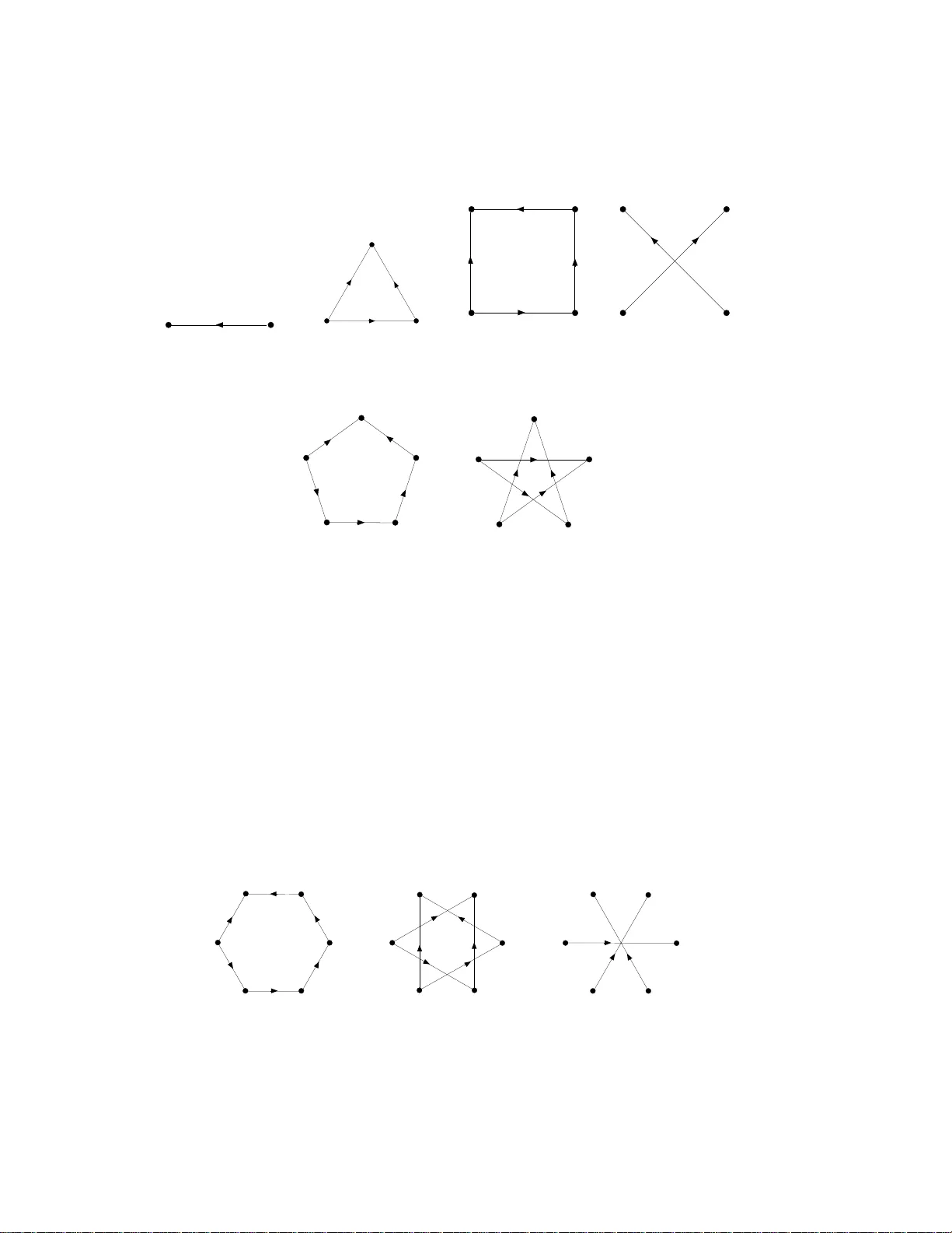
Cluster Mutation-P erio dic Quiv ers and Asso ciated Lauren t Sequences Allan P . F ordy and Rob ert J. Marsh, Sc ho ol of Mathematics, Univ ersit y of Leeds. Leeds LS2 9JT, UK. e-mail: allan@maths.leeds.ac.uk and marsh@maths.leeds.ac.uk Revised v ersion August 2010 Abstract W e consider q uivers/ skew-symmetric matrices under th e action of m utation (in the cluster algebra sense). W e classify those which are isomo rphic to their o wn mutation via a cycle p ermuting all the vertices, and give families of quiver s whic h h a ve h igher p erio dicity . The perio dicity means th at sequences giv en b y recurrence relations arise in a natu ral w a y from the associated cluster algebras. W e presen t a num b er of interesting n ew families of non- linear recurrences, necessarily with the Lauren t prop erty , of b oth the real line and th e plane, conta ining integ rable maps as special cases. In particular, w e sho w that some of th ese re- currences can b e linearised and, with certain initial conditions, give integer sequ ences whic h conta in all solutions of some particular Pell equations. W e ex tend our construction to include recurrences with p ar ameters , giving an explanation of some observ ations made by Gal e. Finally , we p oin t out a connection betw een q uivers whic h arise in our classiﬁcation and t h ose arising in the con text of quive r gauge theories. Keywor ds : cluster alg ebra, quiver mutation, per io dic quiver, Somos seq ue nc e , int eger sequences, Pell’s equation, Laurent ph enomenon, integrable map, linea risation, Seiberg duality , s uper symmetric quiver gauge theory . 1 In tro duction Our main mo tiv ation for this work is the connection betw een cluster a lgebras and integer s e q uences which a re Laurent p olyno mials in their initial ter ms [8]. A key exa mple of this is the Somos 4 sequence, which is given b y the follo wing recur rence: x n x n +4 = x n +1 x n +3 + x 2 n +2 . (1) This formula, with a ppropriate r elab elling of the v a riables, coincides with the cluster exchange relation [7] (recalled b elow; see Section 8) ass o ciated with the vertex 1 in the quiver S 4 of Fig ur e 1(a). Mutation of S 4 at 1 (as in [7 ]; see Deﬁnition 2 .1 below) gives the quiver shown in Figure 1(b) and transfor ms the cluster ( x 1 , x 2 , x 3 , x 4 ) into ( ˜ x 1 , x 2 , x 3 , x 4 ), where ˜ x 1 is given b y x 1 ˜ x 1 = x 2 x 4 + x 2 3 . 1 3 2 1 4 (a) The Somos 4 quiver, S 4 . 1 4 3 2 (b) Mutation of S 4 at 1. Figure 1: The Somos 4 quiv er and its m utation at 1. Remark a bly , a fter this c omplic ate d op er ation of mutation on the quiver, the res ult is a simple rota tion, corres p o nding to the relab elling of indices (1 , 2 , 3 , 4) 7→ (4 , 1 , 2 , 3 ). Therefore, a mutation of the new quiver a t 2 gives the same formula for the exchange relation (up to a relab elling). It is this simple prop erty tha t allows us to think of an inﬁnite sequence o f such mutations as iteration of recurrence (1). In this pap er, we cla ssify quivers with this prop er ty . In this wa y w e o btain a classiﬁca tion o f maps which could b e said to be ‘of Somos type’. In fact we co nsider a mo r e genera l type of “m utation per io dicity”, whic h corr esp onds to Somos type sequences of hig her dimensional s pa ces. It is interesting to no te that many of the quiv ers which hav e occur r ed in the theoretical physics literature co nc e r ning sup ersymmet ric quiver gauge the ories are particular examples fro m our classi- ﬁcation; see for example [5, § 4]. W e spec ula te that some of our other examples ma y b e of in terest in that con text. W e now describ e the conten ts of the ar ticle in mor e detail. In Section 2, we reca ll matrix and quiver m utation from [7], and intro duce the notion o f p erio dicity w e ar e considering. It turns out to b e easier to class ify p erio dic q uivers if we assume tha t cer tain vertices are sinks; we call s uch quivers sink-typ e . In Section 3, w e classify the sink-type quivers of p er io d 1 as nonnegative in teger combinations of a family of primitive quivers. In Section 4, w e do the same for s ink-type p erio d 2 quivers, a nd in Section 5 we classify the sink- t yp e quivers of ar bitr ary perio d. In Section 6, we give a complete cla ssiﬁcation o f all p erio d 1 quivers (without the sink assump- tion), a nd give some examples. It turns out the arbitrary per io d 1 quiv ers can be described in terms of the primitives with N no des, tog e ther with the primitives for quivers with N ′ no des fo r all N ′ less than N o f the s ame parity (Theorem 6.6). In Section 7, w e classify q uivers of p erio d 2 with at most 5 nodes. These descr iptions indicate that a full classiﬁcation for higher p erio d is likely to b e signiﬁcan tly mo re complex than the cla s siﬁcation of perio d 1 quivers. How ever, it is po ssible to co nstruct a la r ge family of p erio d 2 (no t of sink-type) quivers, w hich we present in Section 7.4. In Section 8, we descr ibe the recurr ences that can be ass o ciated to p er io d 1 and p erio d 2 quivers via F omin-Zelevinsky cluster mutation. The nature o f the cluster exchange relation means that the recurrence s w e ha ve asso cia ted to p erio dic quivers are in general nonlinear . How ever, in Sectio n 9, we show that the recurrences as so ciated to per io d 1 primitives can be linearised. This allows us to conclude in Section 9 tha t ce r tain simple linear com binations of subse quences o f the ﬁrst pr imitive per io d 1 quiver (for arbitra rily many no des) provide all the so lutions to an asso c iated Pell equation. In Section 10 we extend our construction of mutation p erio dic quivers to include quivers with 2 fr ozen cluster v ariables , thus enabling the introduction of p ar ameters into the corresp onding recur - rences. As a result, we give a n explanation of some observ ations made by Gale in [1 3]. In Section 11, w e g ive an indication of the connections with sup er symmetric quiver gauge theor ies. In Section 1 2, w e present our ﬁnal conclus io ns. Section 13 is an app endix to Section 9. 2 The P erio dicit y Prop ert y W e cons ider quivers with no 1 cycles or 2 -cycles (i.e. the quivers on which cluster m utation is deﬁned). An y 1- or 2-cy cles whic h a r ise through op erations on the quiver will b e cancelled. The vertices of Q will b e as s umed to lie on the vertices of a regular N -sided poly gon, lab elled 1 , 2 , . . . , N in clo ckwise order. In the usual wa y , we sha ll iden tify a quiver Q , with N no des , with the unique skew-symmetric N × N matrix B Q with ( B Q ) ij given b y the num b er o f arrows from i to j minu s the num b er o f arrows fr om j to i .. W e next recall the deﬁnition of quiver m utation [7 ]. Deﬁnition 2 .1 (Qui ver Mutation) Given a quiver Q we c an mutate at any of its no des. The mutation of Q at no de k , denote d by µ k Q , is c onstructe d (fr om Q ) as follows: 1. R everse al l arr ows which either originate or terminate at no de k . 2. Supp ose that ther e ar e p arr ows fr om n o de i to no de k and q arr ows fr om no de k t o no de j (in Q ). A dd p q arr ows going fr om no de i to n o de j t o any arr ows alr e ady ther e. 3. R emove (b oth arr ows of ) any two-cycles cr e ate d in the pr evious steps. Note that Step 3 is indep endent of any choices made in the remov al o f the tw o-cycle s, since the arrows a re not la be lled. W e a lso note that in Step 2, p q is just the num b er of paths of length 2 betw een nodes i and j which pass through node k . Remark 2. 2 (Matrix Mutation) L et B and ˜ B b e the skew-symmetric matric es c orr esp onding to the quivers Q and ˜ Q = µ k Q . L et b ij and ˜ b ij b e the c orr esp onding matrix ent ries. Then quiver mutation amounts to t he following formula ˜ b ij =  − b ij if i = k or j = k, b ij + 1 2 ( | b ik | b kj + b ik | b kj | ) otherw ise . (2) This is the original formula a ppe aring (in a more genera l con text) in [7 ]. W e n umber the nodes from 1 to N , a rranging them equally spa ced on a circle (clockwise ascend- ing). W e consider the p ermutation ρ : (1 , 2 , · · · , N ) → ( N , 1 , · · · , N − 1). Such a p ermutation a cts on a quiver Q in s uch a w ay that the num b er of arrows fr om i to j in Q is the same a s the num b er of arrows from ρ − 1 ( i ) to ρ − 1 ( j ) in ρQ . T hus the ar rows of Q a re rotated clo ckwise while the no des remain ﬁx ed (alterna tively , this oper ation can be in terpre ted as leaving the arr ows ﬁxed whilst the no des are mo ved in an anticlockwise direc tion). W e will always ﬁx the pos itions of the no des in our diagrams. Note that the action Q 7→ ρQ corre s po nds to the conjugatio n B Q 7→ ρB Q ρ − 1 , where ρ =       0 · · · · · · 1 1 0 . . . . . . . . . . . . 1 0       3 (w e will use the nota tion ρ for both the per m utation and c o rresp onding matrix ). W e consider a sequence o f mutations, starting a t no de 1, follo wed by no de 2, and so on. Mutation at no de 1 of a quiver Q (1) will pro duce a s econd quiver Q (2). The m utation at no de 2 will therefore be of quiver Q (2), giving rise to quiver Q (3) and so on. Deﬁnition 2 .3 We wil l say that a quiver Q has p erio d m if it satisﬁes Q ( m + 1 ) = ρ m Q (1) , with the mutation se quenc e depic te d by Q = Q (1) µ 1 − → Q (2) µ 2 − → · · · µ m − 1 − → Q ( m ) µ m − → Q ( m + 1) = ρ m Q (1) . (3) We c al l the the ab ove se quenc e of quivers the p erio dic chain asso ciate d t o Q . Note that permutations other than ρ m could b e used here , but we do not consider them in this article. If m is minimal in the above, w e s ay that Q is strictly of p erio d m . Also note that each of the quivers Q (1) , . . . , Q ( m ) is o f per io d m (with a renum ber ing of the vertices), if Q is. Recall that a node i of a quiver Q is s aid to b e a sink if all arrows inciden t with i end at i , and is said to be a sour c e if all arrows inciden t with i start at i . Remark 2. 4 (Admis sible sequences) Re c al l that an admissible sequence of sinks in an acyclic quiver Q is a total or dering v 1 , v 2 , . . . , v N of its vertic es such that v 1 is a sink in Q and v i is a sink in µ v i − 1 µ v i − 2 · · · µ v 1 ( Q ) for i = 2 , 3 , . . . , N . Such a se quenc e always has the pr op ert y that µ v N µ v N − 1 · · · µ v 1 ( Q ) = Q [2, § 5.1]. This notion is of imp ortanc e in t he r epr esentation the ory of quivers. We note that if any (n ot ne c essarily acycl ic) qu iver Q has p erio d 1 in our s en se, then µ 1 Q = ρQ . It fol lows that µ N µ N − 1 · · · µ 1 Q = Q . Thus any p erio d 1 quiver has a pr op erty which c an b e r e gar de d as a gener alisation of the notion of ex istenc e of an admissible se quenc e of sinks. In fact, higher p erio d quivers also p ossess this pr op erty pr ovide d the p erio d divid es the numb er of vertic es. 3 P erio d 1 Quiv ers W e now introduce a ﬁnite set of particularly simple quiv ers of p erio d 1, which we shall call the p erio d 1 primitives . Rema rk a bly , it will later b e seen that in a certa in sens e they form a “basis” for the set of all quivers of per io d 1. W e shall also later see that perio d m primitiv es can b e deﬁned as certain sub-quivers of the p erio d 1 primitiv es. Deﬁnition 3 .1 (Period 1 s ink-t yp e quivers) A qu iver Q is said to b e a per io d 1 sink-type quiver if it is of p erio d 1 and no de 1 of Q is a sink. Deﬁnition 3 .2 (Skew-rotat ion) We shal l r efer to the matrix τ =       0 · · · · · · − 1 1 0 . . . . . . . . . . . . 1 0       . as a s kew-rotation . Lemma 3 .3 (P erio d 1 s ink-t yp e equation) A quiver Q with a sink at 1 is p erio d 1 if and only if τ B Q τ − 1 = B Q . 4 Pro of : If no de 1 of Q is a sink, there are no paths of length 2 through it, and the seco nd part of Deﬁnition 2.1 is void. Rev ersa l of the a r rows at no de 1 can be done through a simple conjugation of the matrix B Q : µ 1 B Q = D 1 B Q D 1 , where D 1 = diag( − 1 , 1 , · · · , 1) . Equating this to ρB Q ρ − 1 leads to the equation τ B Q τ − 1 = B Q as requir ed, noting that τ = D 1 ρ.  The map M 7→ τ M τ − 1 simult aneo us ly cyclically per mut es the rows and columns of M (up to a sign), while τ N = − I N , hence τ has order N . This giv es us a method for building pe rio d 1 matric e s: we s um ov er τ -orbits. The p erio d 1 primitiv es P ( k ) N . W e consider a quiver with just a single arrow from N − k + 1 to 1, represented b y the sk ew-symmetric matrix R ( k ) N with ( R ( k ) N ) N − k +1 , 1 = 1 , ( R ( k ) N ) 1 ,N − k +1 = − 1 and ( R ( k ) N ) ij = 0 otherwise. W e deﬁne sk ew-symmetric matric e s B ( k ) N as follows: B ( k ) N = ( P N − 1 i =0 τ i R ( k ) N τ − i , if N = 2 r + 1 and 1 ≤ k ≤ r, or if N = 2 r and 1 ≤ k ≤ r − 1; P r − 1 i =0 τ i R ( r ) N τ − i , if k = r and N = 2 r . (4) Let P ( k ) N denote the quiver corresp onding to B ( k ) N . W e re ma rk that the geometric action of τ in the ab ov e s um is to ro tate the a rrow clo ckwise without change of or ient ation, except that when the tail of the arrow ends up at no de 1 it is reversed. It follows that 1 is a s ink in the resulting quiver. Since it is a s um ov er a τ -orbit, we hav e τ B ( k ) N τ − 1 = B ( k ) N , and thus that P ( k ) N is a p erio d 1 s ink-type quiver. In fact, w e ha ve the simple description: B ( k ) N =  τ k − ( τ t ) k , if N = 2 r + 1 and 1 ≤ k ≤ r, or N = 2 r and 1 ≤ k ≤ r − 1; τ r , if N = 2 r and k = r . where τ t denotes the tr a nsp ose of τ . Note that we have restricted to the choice 1 ≤ k ≤ r b ecause when k > r , our construction g ives nothing new. Fir s tly , consider the case N 6 = 2 k . Then B ( N +1 − k ) N = B ( k ) N , b ecaus e the primitive B ( k ) N has ex actly tw o ar rows ending at 1: those star ting at k + 1 a nd at N + k − 1. Starting with either of these arr ows pro duces the same result. If N = 2 k , these t wo ar rows are identical, and since τ k is skew-symmetric, τ k − ( τ t ) k = 2 τ k . The sum ov er N = 2 k terms just go es t wice ov er the sum ov er k terms. In this co ns truction w e could e q ually w ell hav e chosen no de 1 to be a source. W e would then hav e R ( k ) N 7→ − R ( k ) N , B ( k ) N 7→ − B ( k ) N and P ( k ) N 7→ ( P ( k ) N ) opp , where Q opp denotes the opp o site quiv er of Q (with all a r rows reversed). Our o riginal motiv ation in terms of sequences with the Laurent prop erty is derived through c luster exchange relations, which do not distinguish b etw een a quiver and its o ppo site, so we consider these as equiv alent. Remark 3. 4 We note that e ach primi tive is a disjo int u n ion of cycles or arr ows, i.e. quivers whose underlying gr aph is a union of c omp onent s which ar e either of typ e A 2 or of typ e e A m for some m . Figures 2 to 4 show the per io d 1 pr imitives we ha ve co nstructed, for 2 ≤ N ≤ 6. 5 2 1 (a) P (1) 2 2 3 1 (b) P (1) 3 4 1 2 3 (c) P (1) 4 3 1 2 4 (d) P (2) 4 Figure 2: The p erio d 1 primitiv es for 2, 3 and 4 nodes. 5 1 2 3 4 (a) P (1) 5 4 5 1 2 3 (b) P (2) 5 Figure 3: The p erio d 1 pr imitives for 5 no des. Remark 3. 5 (An In v olution ι : Q 7→ Q opp ) It is e asily s e en that the fol lowing p ermu tation of the no des is a symmetry of the pri mitives P ( i ) N (if we c onsider Q and Q opp as e quivalent): ι : (1 , 2 , · · · , N ) 7→ ( N , N − 1 , · · · , 1) . In matrix language, this fol lows fr om the facts that ιR ( k ) N ι = − R ( k ) N and ιτ ι = τ t , wher e ι =     0 1 . . . . . . 1 0     . It is inter esting to note that ρ is a Coxeter element in Σ N r e gar de d as a Coxeter gr oup, while ι is the longest element . 5 6 1 2 3 4 (a) P (1) 6 6 1 2 3 4 5 (b) P (2) 6 6 1 2 3 4 5 (c) P (3) 6 Figure 4: The p erio d 1 pr imitives for 6 no des. 6 W e ma y combine primitiv es to fo rm more co mplicated quivers. Consider the sum P = r X i =1 m i P ( i ) N , where N = 2 r or 2 r + 1 for r a n integer and the m i are arbitrar y integers. It is easy to see that the corres p o nding quiver is a p erio d 1 sink -type quiver whenev er m i ≥ 0 for a ll i . I n fact, we ha ve: Prop ositio n 3.6 (Class i ﬁcation of p erio d 1 sink-type quiv ers) Le t N = 2 r or 2 r + 1 , wher e r is an inte ger. Every p erio d 1 sink-typ e quiver with N no des has c orr esp onding matrix of the form B = P r k =1 m k B ( k ) N , wher e the m k ar e arbitr ary nonne gative inte gers. Pro of : Let B be the matrix o f a p erio d 1 sink-t yp e quiver. It remains to show that B is of the form stated. W e no te that conjugation by τ p ermutes the set of summands appe aring in the deﬁnition (4) of the B ( k ) N , i.e. the elements τ i R ( k ) N τ − i for 0 ≤ i ≤ N − 1 and 1 ≤ k ≤ r if N = 2 r + 1, for 0 ≤ i ≤ N − 1 a nd 1 ≤ k ≤ r − 1 if N = 2 r , together with the elements τ i R ( r ) N τ − i for 0 ≤ i ≤ r − 1 if N = 2 r . These 1 2 N ( N − 1) elements ar e easily seen to form a basis of the space of real skew-symmetric matrices. By Lemma 3.3 , τ B τ − 1 = B , so B is a linea r com bination of the perio d 1-primitives (which are the orbit sums for the conjuga tion action o f τ on the a b ove bas is), B = P r k =1 m k B ( k ) N . The suppo rt of the B ( k ) N for 1 ≤ k ≤ r is distinct, so B N − k +1 , 1 = m k for 1 ≤ k ≤ r (where the support of a matrix is the set of p ositions of its non- zero entries). Hence the m k are int eger s, as B is a n int eger matrix. Since B is sink-type, all the m k m ust be no nnegative.  Note that this means all p erio d 1 sink-type quivers are inv a riant under ι in the ab ove sense. W e also note that if the m k are taken to be of mixed sig n, then Q is no longer p erio dic without the addition of fur ther “corr ection” terms . Theor em 6.6 gives these cor rection terms. 4 P erio d 2 Quiv ers Period 2 primitives will b e deﬁned in a simila r wa y . First, we make the following deﬁnitio n: Deﬁnition 4 .1 (Period 2 s ink-t yp e quivers) A qu iver Q is said to b e a per io d 2 sink-type quiver if it is of p erio d 2 , no de 1 of Q (1) = Q is a sink, and no de 2 of Q (2) = µ 1 Q is a sink. Let Q b e a p er io d 2 q uiver. Then we hav e tw o q uivers in o ur p erio dic chain (3), Q (1) and Q (2) = µ 1 Q , with corr e spo nding matr ices B (1 ) , B (2). If Q (1) is of sink-type then, since no de 1 is a sink in Q (1 ), the mutation Q (1) 7→ µ 1 Q (1) = Q (2) a gain only inv olves the r eversal of arrows at no de 1. Similarly , since no de 2 is a sink for Q (2), the mutation Q (2) 7→ µ 2 Q (2) only in volv es the reversal o f arr ows at no de 2. Obviously each p er io d 1 quiver Q is also p er io d 2 , wher e B (2) = ρB (1) ρ − 1 . How e ver, we will construct some s trictly p erio d 2 primitiv es. As b e fo re, we hav e: Lemma 4 .2 (P erio d 2 s ink-t yp e equation) Supp ose that Q is a quiver with a sink at 1 and that Q (2) has a sink at 2 . Then Q is p erio d 2 if and only if τ 2 B Q τ − 2 = B Q . Pro of : As b efor e , rev ersa l of the arrows at no de 1 of Q can b e achieved throug h a simple conjugation of its matrix: µ 1 B Q = D 1 B Q D 1 . Similarly , rev ersa l of the arrows at no de 2 o f Q (2 ) can be achiev ed through µ 2 B Q (2) = D 2 B Q (2) D 2 , where D 2 = diag(1 , − 1 , 1 , · · · , 1) = ρD 1 ρ − 1 . 7 Equating the compos ition to ρ 2 B Q ρ − 2 leads to the equation B Q = D 1 D 2 ρ 2 B Q ρ − 2 D 2 D 1 = τ 2 B Q τ − 2 .  F ollowing the same pro cedure as for p erio d 1, we need to form orbit-sums for τ 2 on the basis considered in the previous section; we shall c a ll these p erio d 2 primitiv es. A τ -or bit of o dd car dinality is also a τ 2 -orbit, so the or bit sum will be a per io d 2 pr imitiv e which is a ls o of p er io d 1. Thus w e cannot hop e to get perio d 2 solutions whic h a re not also p erio d 1 solutions unless there a re an even n umber of no des. A τ -orbit of even cardinality splits into t wo τ 2 -orbits. When N = 2 r , the matrices R ( k ) N , for 1 ≤ k ≤ r − 1, gener a te strictly p e rio d 2 primitiv es P ( k, 1) N , 2 , with matrices giv en by B ( k, 1) N , 2 = r − 1 X i =0 τ 2 i R ( k ) N τ − 2 i , If, in addition, N is divisible b y 4, we obtain the additional strictly p er io d 2 primitives P ( r, 1) N , 2 , with matrices given by: B ( r, 1) N , 2 = r / 2 − 1 X i =0 τ 2 i R ( r ) N τ − 2 i . Geometrically , the primitive P ( k, 1) N , 2 is obtained from the pe rio d 1 primitive P ( k ) N by “removing half the ar rows” (the ones corr esp onding to o dd powers of τ ). The r emov ed arrows form a nother per io d 2 primitiv e, called P ( k, 2) N , 2 , which ma y b e deﬁned as the matr ix: B ( k, 2) N , 2 = τ B ( k, 1) N , 2 τ − 1 . W e mak e the following observ ation: Lemma 4 .3 We have ρ − 1 µ 1 B ( k, 1) N , 2 ρ = B ( k, 2) N , 2 for 1 ≤ k ≤ r . Pro of : F o r 1 ≤ k ≤ r − 1, we hav e ρ − 1 µ 1 B ( k, 1) N , 2 ρ = ρ − 1 D 1 B ( k, 1) N , 2 D − 1 1 ρ = τ − 1 r − 1 X i =0 τ 2 i R ( k ) N τ − 2 i ! τ = τ r − 1 X i =0 τ 2 i − 2 R ( k ) N τ 2 − 2 i ! τ − 1 , since ρ − 1 D 1 = τ − 1 . Since τ − 2 = − τ 2 r − 2 , w e hav e ρ − 1 B ( k, 1) N , 2 (2) ρ = τ B ( k, 1) N , 1 τ − 1 = B ( k, 2) N , 2 . A similar argument holds for k = r , noting that in this case, τ − 2 R ( k ) N = τ r − 2 R ( k ) N .  Figures 5 and 6 show the strictly p erio d 2 primitiv es with 4 and 6 no des. W e need the following: 8 4 1 2 3 (a) P (1 , 1) 4 , 2 2 3 4 1 (b) P (1 , 2) 4 , 2 4 1 2 3 (c) P (2 , 1) 4 , 2 4 1 2 3 (d) P (2 , 2) 4 , 2 Figure 5: The strictly perio d 2 primitives for 4 no des. 5 6 1 2 3 4 (a) P (1 , 1) 6 , 2 5 6 1 2 3 4 (b) P (1 , 2) 6 , 2 6 1 2 3 4 5 (c) P (2 , 1) 6 , 2 6 1 2 3 4 5 (d) P (2 , 2) 6 , 2 Figure 6: The p erio d 2 primitiv es for 6 no des Lemma 4 .4 (a) Le t M b e an N × N skew-symmetric matrix with M ij ≥ 0 whenever i ≥ j . Then τ M τ − 1 has the same pr op erty. (b) Al l p erio d 2 primitives B ( k,l ) N , 2 have nonne gative entries b elow the le ading diago nal. Pro of : W e m ust a lso hav e M ij ≤ 0 for i ≤ j . W e ha ve ( τ M τ − 1 ) ij =          M i − 1 ,j − 1 i > 1 , j > 1 , − M N ,j − 1 i = 1 , j > 1 , − M i − 1 ,N i > 1 , j = 1 , M N ,N i = 1 , j = 1 . from which (a) follows. Part (b) follows from part (a) and the deﬁnition of the p erio d 2 primitives.  As in the p erio d 1 case, we obtain p erio d 2 sink-type quivers by ta king orbit-sums of the basis elements: Prop ositio n 4.5 (Class i ﬁcation of p erio d 2 sink-type quiv ers) I f N is o dd, ther e ar e no strictly p erio d 2 sink-typ e quivers with N no des. If N = 2 r is an even inte ger t hen every st rictly p erio d 2 sink-typ e quiver with N no des has c orr esp onding matrix of the form B = ( P r k =1 P 2 j =1 m kj B ( k,j ) N , 2 if 4 | N , ( P r − 1 k =1 P 2 j =1 m kj B ( k,j ) N , 2 ) + m r 1 B ( r ) N if 4 ∤ N , wher e the m j k ar e arbitr ary nonne gative inte gers such that if 4 | N , ther e is at le ast one k , 1 ≤ k ≤ r , such that m k 1 6 = m k 2 , and if 4 ∤ N , ther e is at le ast one k , 1 ≤ k ≤ r − 1 , such that m k 1 6 = m k 2 . 9 Pro of : Using the above discussion and an argument similar to that in the p erio d 1 case, we obtain an express io n as above for B for which the m kj are integers. It is easy to chec k that each primitiv e has a non-zero entry in the ﬁrst or second column, below the leading diago na l. B y Lemma 4.4, this ent ry must b e p ositive. If the en try is in the ﬁr s t column, the corresp onding m kj m ust b e nonegative as 1 is a sink. If it is in the seco nd column then, since 1 is a s ink, mutation at 1 do e s not aﬀect the ent ries in the se cond co lumn below the leading diagonal. Since a fter mutation at 1, 2 is a sink, the corres p o nding m kj m ust be no nnegative in this case also.  Whilst the form ulae above dep end upon par ticular character istics of the primitives, i.e. having a sp eciﬁc sink, a s imilar relatio n exis ts for any p er io d 2 quiver. F o r an y quiver Q (rega rdless o f any symmetry or p erio dicit y pro pe r ties), we hav e µ k +1 ρ Q = ρ µ k Q , which just corr esp onds to relab elling the no de s . W e write this sy m b olically a s µ k +1 ρ = ρµ k and ρ − 1 µ k +1 = µ k ρ − 1 . F o r the per io d 2 case, the per io dic chain (3) can b e written as: Q (1) µ 1 − → Q (2) µ 2 − → Q (3) = ρ 2 Q (1) µ 3 − → Q (4) = ρ 2 Q (2) µ 4 − → · · · Whilst µ 1 and µ 2 are genuinely diﬀerent mutations, µ 3 and µ 4 are just µ 1 and µ 2 after r elab elling. Since ρ − 1 µ 2 Q (2) = ρQ (1), we ha ve µ 1 ( ρ − 1 Q (2)) = ρQ (1). W e also have µ 2 ( ρ Q (1)) = ρ µ 1 Q (1) = ρ Q (2). Since Q (3 ) = µ 2 Q (2) = ρ 2 Q (1), we hav e ρ − 1 µ 2 Q (2) = ρQ (1 ), and thus we obtain µ 1 ( ρ − 1 Q (2)) = ρQ (1 ). W e th us ca n extend the a bove diagram to that in Figure 7. ρ − 1 Q (2) ρ Q (1) ρ Q (2) Q (1) Q (2) ρ 2 Q (1) ρ 2 Q (2) ✲ ✲ ✲ ✲ ✲ ✲ ✲ ◗ ◗ ◗ ◗ ◗ ◗ ❦ ◗ ◗ ◗ ◗ ◗ ◗ ❦ ◗ ◗ ◗ ◗ ◗ ◗ ❦ µ 1 µ 2 µ 3 µ 1 µ 2 µ 3 µ 4 ρ − 1 ρ − 1 ρ − 1 Figure 7: Perio d 2 quivers and m utations If Q (1) , Q (2) have sinks at no des 1 and 2 r e spe ctively , then s o do ρ − 1 Q (2) and ρ Q (1) and the m utations µ 1 and µ 2 in the ab ov e diag ram act line arly . This gives µ 1 ( Q (1) + ρ − 1 Q (2)) = Q (2) + ρ Q (1) = ρ ( Q (1) + ρ − 1 Q (2)) and µ 2 ( Q (2) + ρ Q (1)) = ρ 2 Q (1) + ρ Q (2) = ρ ( Q (2) + ρ Q (1)) , so Q (1) + ρ − 1 Q (2) is p er io d 1. W e ha ve proved the follo wing: Prop ositio n 4.6 L et Q b e p erio d 2 s ink- t yp e quiver. Then Q (1) + ρ − 1 Q (2) is a quiver of p erio d 1 . 5 Quiv ers with Higher Pe rio d Higher p erio d primitives are deﬁned in a similar way . The p erio dic chain (3) contains m quivers Q (1) , Q (2) , . . . , Q ( m ), with corresp onding matrices B (1) , · · · , B ( m ). 10 Deﬁnition 5 .1 (Period m si nk-t yp e quiv ers) A quiver Q is said to b e a p er io d m sink-type quiver if it is of p erio d m and, for 1 ≤ i ≤ m , no de i of Q ( i ) is a sink. Thu s the m utation Q ( i ) 7→ Q ( i + 1) = µ i Q ( i ) ag ain only inv olves the reversal of arrows at node i , so ca n be a chiev ed through a simple conjugation of its matrix: µ i B ( i ) = D i B ( i ) D i . Here D i = diag(1 , · · · , 1 , − 1 , 1 , · · · , 1 ) = ρ i − 1 D 1 ρ − i +1 (with a “ − 1” in the i th position). As in the perio d 1 and 2 cases , w e obtain: Lemma 5 .2 (P erio d m sink-t yp e e quation) Su pp ose that Q is a quiver with a sink at the i th no de of Q ( i ) for i = 1 , 2 , . . . , m . Then Q is p erio d m if and only if τ m B Q τ − m = B Q . Pro of : W e have that Q ha s p erio d m if a nd only if D m · · · D 1 B Q D 1 · · · D m = ρ m B Q ρ − m , i.e. if and only if B Q = D 1 · · · D m ρ m B Q ρ − m D m · · · D 1 = τ m B Q τ − m .  Starting with the same matrices R ( k ) N , we now use the action M 7→ τ m M τ − m to build a n inv ar iant, i.e. we take orbit sums for τ m . W e only obtain strictly m -p erio dic elements in the case where the o rbit has size divisible by m . When m | N , the matrices R ( k ) N , for 1 ≤ k ≤ r − 1 (where N = 2 r or 2 r + 1, r an integer), gener ate per io d m pr imitiv es B ( k, 1) N ,m , with ma trices given b y B ( k, 1) N ,m = ( N/m ) − 1 X i =0 τ mi R ( k ) N τ − mi . Geometrically , the primitive P ( k, 1) N ,m is obtained from the primitive P ( k ) N by o nly including every m th arrow. As b efor e, we form a nother m − 1 p er io d m primitives, P ( k,j ) N ,m for j = 2 , . . . , m , with ma tr ices given b y: B ( k,j ) N ,m = τ j − 1 B ( k, 1) N ,m ( τ j − 1 ) − 1 . Note that the elements τ l R ( k ) N τ − l , fo r 0 ≤ l ≤ N − 1, form a τ -or bit of size N . Since m | N , this breaks up into m τ m -orbits each of size N /m ; the elemen ts abov e are the o rbit sums. Similarly , if (2 m ) | N (so we a re in the case N = 2 r ) then the τ m -orbit-sum o f R ( r ) N is B ( k, 1) N ,m = ( N/ 2 m ) − 1 X i =0 τ mi R ( r ) N τ − mi . with co rresp onding quiver P ( k, 1) N ,m . W e also obta in a nother m − 1 p er io d m pr imitiv es, P ( r,j ) N ,m , for j = 2 , . . . , m , with ma trices B ( r,j ) N ,m = τ j − 1 B ( r, 1) N ,m ( τ j − 1 ) − 1 . As in the p erio d 1 a nd 2 cases, w e o btain a rbitrary s tr ictly p erio d m sink-type quivers by taking orbit-sums of the bas is elemen ts. The nonnegativ ity of the co eﬃcients m kj is shown in a similar w ay also. 11 Prop ositio n 5.3 (Class i ﬁcation of p erio d m sink-type quiv ers) If m ∤ N , t her e ar e no strictly p erio d m sink-typ e quivers. If (2 m ) | N , the gener al strictly p erio d m sink-t yp e quiver is of t he form B = r X k =1 m X j =1 m kj B ( k,j ) N ,m , wher e t he m kj ar e nonne gative inte gers and t her e is at le ast one k , 1 ≤ k ≤ r , for which the m kj ar e not al l e qual. If m | N but (2 m ) ∤ N then the gener al p erio d m sink-typ e quiver has the form B = ( P r k =1 P m j =1 m kj B ( k,j ) N ,m if N = 2 r + 1 is o dd; P r − 1 k =1 P m j =1 m kj B ( k,j ) N ,m + P m/ 2 j =1 m r j B ( r,j ) N ,m/ 2 if N = 2 r is even, wher e the m kj ar e nonne gative inte gers and whe r e in the ﬁrst c ase, ther e is at le ast one k , 1 ≤ k ≤ r , for which the m kj ar e not al l e qual, and in the se c ond c ase, ther e is at le ast one k , 1 ≤ k ≤ r − 1 , for which the m kj ar e not al l e qual. As b efore , we use µ k +1 ρ = ρµ k and ρ − 1 µ k +1 = µ k ρ − 1 , from which it follows that µ k ρ − j = ρ − j µ k + j . In turn, this g ives µ k ( ρ − j Q ( j + k )) = ρ − j µ j + k Q ( j + k ) = ρ − j Q ( j + k + 1) . Suppo se now that Q is a p erio d m quiver. Then we have Q ( sm + j ) = ρ sm Q ( j ) for 1 ≤ j ≤ m . W e use this to extend the p er io dic chain (3) to an m lev el arr ay . W e have µ 1 ( ρ − j Q ( j + 1 )) = ρ − j Q ( j + 2) , µ 2 ( ρ − j Q ( j + 2 )) = ρ − j Q ( j + 3) , . . . , arriving at µ m ( ρ − j Q ( j + m ) = ρ − j Q ( j + m + 1) = ρ m ( ρ − j Q ( j + 1)) . W e write this p erio d m sequence in the j th level of the arr ay , i.e. ρ − j Q ( j + 1) µ 1 − → ρ − j Q ( j + 2) µ 2 − → · · · µ m − 1 − → ρ − j Q ( j + m ) µ m − → ρ m ( ρ − j Q ( j + 1 )) . Again w e have that if Q ( j ) has a sink at no de j for each j , then each ρ − j Q ( j + 1) has a sink at no de 1 a nd the mutation µ 1 acts linearly . This g ives µ 1 ( Q (1) + ρ − 1 Q (2) + · · · + ρ − m +1 Q ( m )) = ρ ( Q (1) + ρ − 1 Q (2) + · · · + ρ − m +1 Q ( m )) , so Q (1) + ρ − 1 Q (2) + · · · + ρ − m +1 Q ( m ) is p erio d 1. W e ha ve proved: Prop ositio n 5.4 L et Q b e p erio d m sink-typ e quiver. Then Q (1) + ρ − 1 Q (2) + · · · + ρ − m +1 Q ( m ) is a quiver of p erio d 1 . Example 5. 5 (P erio d 3 Primitives) P ro ceeding as describ ed ab ov e, whenever N is a m ultiple of 3 we obtain 3 p erio d 3 primitiv es for ea ch p erio d 1 primitiv e. Figure 8 sho ws those with 6 no des. 12 5 6 1 2 3 4 (a) P (1 , 1) 6 , 3 5 6 1 2 3 4 (b) P (1 , 2) 6 , 3 5 6 1 2 3 4 (c) P (1 , 3) 6 , 3 6 1 2 3 4 5 (d) P (2 , 1) 6 , 3 6 1 2 3 4 5 (e) P (2 , 2) 6 , 3 6 1 2 3 4 5 (f ) P (2 , 3) 6 , 3 6 1 2 3 4 5 (g) P (3 , 1) 6 , 3 6 1 2 3 4 5 (h) P (3 , 2) 6 , 3 6 1 2 3 4 5 (i) P (3 , 3) 6 , 3 Figure 8: The p erio d 3 pr imitives for 6 no des. 6 P erio d 1 General Solution In this section w e give an explicit constr uc tio n of the N × N skew-symmetric matrices c o rresp onding to arbitrar y p erio d 1 quivers, i.e. those for which mutation at no de 1 has the s ame eﬀect a s the rotation ρ . W e express the general so lution as an explicit sum of perio d 1 primitives, thus giving a simple clas siﬁcation of all s uch quivers. In anticipation of the ﬁnal r esult, we consider the following matrix: B =      0 − m 1 · · · − m N − 1 m 1 0 ∗ . . . 0 m N − 1 ∗ 0      . (5) Using (2), the general mu tation rule at no de 1 is ˜ b ij =  − b ij if i = 1 or j = 1 , b ij + 1 2 ( | b i 1 | b 1 j + b i 1 | b 1 j | ) otherw ise . (6) The eﬀect o f the rota tio n B 7→ ρB ρ − 1 is to move the entries of B down and right one step, so that ( ρB ρ − 1 ) ij = b i − 1 ,j − 1 , r emembering that indice s are la be lled mo dulo N , so N + 1 ≡ 1. F or 13 1 ≤ i, j ≤ N − 1, let ε ij = 1 2 ( m i | m j | − m j | m i | ) . Then if m i and m j hav e the sa me sign, ε ij = 0. Other wis e ε ij = ±| m i m j | , where the sign is tha t o f m i . Let e B = µ 1 B , so that ˜ b ij = b ij + ε i − 1 ,j − 1 . Theorem 6.1 L et B b e an N × N skew-symmetric inte ger matrix. L et b k 1 = m k − 1 for k = 2 , 3 , . . . , N . Then µ 1 B = ρB ρ − 1 if and only if m r = m N − r for r = 1 , 2 , . . . , N − 1 , b ij = m i − j + ε 1 ,i − j +1 + ε 2 ,i − j +2 + · · · + ε j − 1 ,i − 1 for al l i > j , and B is symmetric along the non-le ading diagonal . Pro of : By skew-symmetry , we note that w e only need to deter mine b ij for i > j . W e need to so lve µ 1 B = ρB ρ − 1 . By the above discussion, this is e quiv alent to solv ing b ij + ε i − 1 ,j − 1 = b i − 1 ,j − 1 , (7) for i > j , with ε ij as given ab ov e. So lving the eq uation leads to a recursive form ula for b ij . W e obtain b ij = b i − 1 ,j − 1 + ε j − 1 ,i − 1 = b i − 2 ,j − 2 + ε j − 1 ,i − 1 + ε j − 2 ,i − 2 . . . = b i − j +1 , 1 + ε j − 1 ,i − 1 + ε j − 2 ,i − 2 + · · · + ε 1 ,i − j +1 . In particular, we hav e: b N j = m N − j + ε 1 ,N − j +1 + ε 2 ,N − j +2 + · · · + ε j − 2 ,N − 2 + ε j − 1 ,N − 1 . (8) W e also hav e that m j = ˜ b 1 ,j +1 = ( ρB ρ − 1 ) 1 ,j +1 = b N j . In particular, m 1 = b N 1 = m N − 1 . E quation 8 gives m 2 = b N 2 = m N − 2 + ε 1 ,N − 1 = m N − 2 + ε 11 = m N − 2 . So m 2 = m N − 2 . Supp ose that we ha ve shown that m j = m N − j for j = 1 , 2 , . . . , r . Then equation 8 gives b N ,r +1 = m N − r − 1 + ε 1 ,N − r + ε 2 ,N − r +1 + · · · + ε r,N − 1 = m N − r − 1 + r X i =1 ε i,N − r + i − 1 = m N − r − 1 + r X i =1 ε i,r +1 − i = m N − r − 1 + ε 1 ,r + ε 2 ,r − 1 + · · · + ε r, 1 = m N − r − 1 , using the inductive hypothesis and the fact that ε st = − ε ts for all s, t . Hence m r +1 = m N − r − 1 and we have b y induction that m r = m N − r for 1 ≤ r ≤ N − 1. W e ha ve, for i > j , b y equatio n (8), b N − j +1 ,N − i +1 = m ( N − j +1) − ( N − i +1) + ε ( N − i +1) − 1 , ( N − j +1) − 1 + ε ( N − i +1) − 2 , ( N − j +1) − 2 + · · · + ε 1 , ( N − j +1) − ( N − i +1)+1 = m i − j + ε N − i,N − j + ε N − i − 1 ,N − j − 1 + · · · + ε 1 ,i − j +1 , 14 and we hav e, again using (8) and the fact that ε N − a , N − b = ε ab , m i − j = m N − i + j = b N ,N − i + j = b N − j +1 ,N − i +1 + ε N − i + j − 1 , N − 1 + ε N − i + j − 2 , N − 2 + · · · + ε N − i +1 ,N − j +1 = b N − j +1 ,N − i +1 + ε i − j +1 , 1 + ε i − j +2 , 2 + · · · + ε i − 1 ,j − 1 , so b N − j +1 ,N − i +1 = m i − j + ε j − 1 ,i − 1 + · · · + ε i − j +2 , 2 + ε 1 ,i − j +1 = b ij . Hence B is symmetric a lo ng the no n-leading diagonal. If B satisﬁes all the requirements in the statemen t of the theorem, then equation 8 is satisﬁed, and therefore ρB ρ − 1 = µ 1 B . The pr o of is complete.  W e rema rk that with the identiﬁcation m r = m N − r , we have seen that the formula (8) has a symmetry , due to whic h the ε ’s cancel in pairwise fashion: b N ,N − k +1 = b k 1 + ε 1 k + ε 2 ,k +1 + · · · + ε k +1 , 2 + ε k 1 The formula (8) is just a tr uncation of this, so not all ter ms cancel. As we march from b k 1 in a “south e asterly dire c tio n”, we ﬁrst a dd ε 1 k , ε 2 ,k +1 , etc, un til w e r each ε r,r +1 (when N − k = 2 r ) or ε r r = 0 (when N − k = 2 r + 1). At this stage we start to subtract terms on a basis of “last in, ﬁr s t out”, with the result that the matrix has reﬂective symmetry ab out the second diagonal a s w e ha ve seen. Remark 6. 2 (Sink-type case) We n ote that if al l the m i have the same s ign, then al l the ε ij ar e zer o. Equation (7) r e duc es to b ij = b i − 1 ,j − 1 and we r e c over the sink-typ e p erio d 1 solutions c onsider e d in Pr op osition 3.6. 6.1 Examples The simplest no ntrivial example is when N = 4. Example 6. 3 (P erio d 1 Quiv er with 4 No des ) Her e the matrix has the form B =     0 − m 1 − m 2 − m 1 m 1 0 − m 1 − ε 12 − m 2 m 2 m 1 + ε 12 0 − m 1 m 1 m 2 m 1 0     , As pr eviously noted, if m 1 and m 2 hav e the sa me sig n, then ε 12 = 0 and this matr ix is just the sum of primitives for 4 no des . The 2 × 2 matrix in the “centre” of B (formed out of rows and columns 2 and 3),  0 − ε 12 ε 12 0  , corres p o nds to ε 12 times the primitive P (1) 2 with 2 no des (see Figure 2). F or the case m 1 = 1 , m 2 = − 2 , ε 12 = 2, we obtain the Somos 4 quiver in Figure 1(a). The ac tio n of ι (see Rema rk 3.5) is 1 ↔ 4 , 2 ↔ 3 and clearly just reverses all the arrows as predicted by Remark 3.5. 15 Example 6. 4 (P erio d 1 Quiv er with 5 No des ) Her e the general per io d 1 solution has the form B =       0 − m 1 − m 2 − m 2 − m 1 m 1 0 − m 1 − ε 12 − m 2 − ε 12 − m 2 m 2 m 1 + ε 12 0 − m 1 − ε 12 − m 2 m 2 m 2 + ε 12 m 1 + ε 12 0 − m 1 m 1 m 2 m 2 m 1 0       which can be written as B = 2 X k =1 m k B ( k ) 5 + ε 12 B (1) 3 , where B (1) 3 is embedded symmetrically in the middle of a 5 × 5 matr ix (surrounded by zeros). When m 1 = 1 and m 2 = − 1, this matrix c o rresp onds to the Somos 5 sequence; see Figure 9 for the cor r esp onding quiver. 1 2 3 4 5 Figure 9: The So mos 5 quiver. Example 6. 5 (P erio d 1 Quiv er with 6 No des ) Her e the matrix has the form B =         0 − m 1 − m 2 − m 3 − m 2 − m 1 m 1 0 − m 1 − m 2 − m 3 − m 2 m 2 m 1 0 − m 1 − m 2 − m 3 m 3 m 2 m 1 0 − m 1 − m 2 m 2 m 3 m 2 m 1 0 − m 1 m 1 m 2 m 3 m 2 m 1 0         +         0 0 0 0 0 0 0 0 − ε 12 − ε 13 − ε 12 0 0 ε 12 0 − ε 12 − ε 13 0 0 ε 13 ε 12 0 − ε 12 0 0 ε 12 ε 13 ε 12 0 0 0 0 0 0 0 0         +         0 0 0 0 0 0 0 0 0 0 0 0 0 0 0 − ε 23 0 0 0 0 ε 23 0 0 0 0 0 0 0 0 0 0 0 0 0 0 0         , which can be written as B = 3 X j =1 m k B ( k ) 6 + 2 X k =1 ε 1 ,k +1 B ( k ) 4 + ε 23 B (1) 2 , where the p erio dic solutions with fewer rows and columns are embedded sy mmetr ically within a 6 × 6 matrix. 16 6.2 The Period 1 General Solution in T erms of Primitiv es It ca n be s een from the ab ov e exa mples that the solutions ar e built out of a seq uence of sub- matrices, each of which corr esp onds to o ne of the primitives. The main matr ix is just an integer linear combination o f primitive matrices for the full set o f N nodes. The next ma trix is a c ombination (with co eﬃcients ε 1 j ) of primitive matr ic es for the N − 2 nodes 2 , · · · , N − 1. W e con tinue to reduce by 2 un til we reach either 2 no des (when N is even) or 3 no des (when N is odd). Remark a bly , as can be se e n from the general s tructure of the matrix given by (8), to g ether with the symmetry m N − r = m r , this descr iption holds fo r all N . Recall that for a n even (or o dd) num b er of no des, N = 2 r (o r N = 2 r + 1), there are r primitives , lab elled B ( k ) 2 r (or B ( k ) 2 r + 1 ), k = 1 , · · · , r . W e denote the genera l linear combination of these by e B 2 r ( µ 1 , · · · , µ r ) = r X j =1 µ j B ( j ) 2 r , or e B 2 r + 1 ( µ 1 , · · · , µ r ) = r X j =1 µ j B ( j ) 2 r + 1 , for integers µ j . The quivers co r resp onding to e B 2 r ( µ 1 , · · · , µ r ) and e B 2 r + 1 ( µ 1 , · · · , µ r ) (i.e. without the extr a terms coming from the ε ij ) do not ha ve per io dicit y pro pe rties (in g e ne r al). W e no w restate Theor em 6.1 in this new notation: Theorem 6.6 (The gen e ral p erio d 1 quiv er) L et B 2 r (r esp e ctively B 2 r + 1 ) denote the matrix c orr esp onding t o the gener al even (r esp e ctively o dd) no de quiver of mutation p erio dicity 1 . Then 1. B 2 r = e B 2 r ( m 1 , · · · , m r ) + r − 1 X k =1 e B 2( r − k ) ( ε k,k +1 , · · · , ε kr ) , wher e the matrix e B 2( r − k ) ( ε k,k +1 , · · · , ε kr ) is emb e dde d in a 2 r × 2 r matrix in r ows and c olumns k + 1 , · · · , 2 r − k . 2. B 2 r + 1 = e B 2 r + 1 ( m 1 , · · · , m r ) + r − 1 X k =1 e B 2( r − k )+1 ( ε k,k +1 , · · · , ε kr ) , wher e the matrix e B 2( r − k )+1 ( ε k,k +1 , · · · , ε kr ) is emb e dde d in a 2 r + 1 × 2 r + 1 matrix in r ows and c olumns k + 1 , · · · , 2 r + 1 − k . 7 Quiv ers with Mutation P erio dicit y 2 Already at per io d 2, we cannot g ive a full class iﬁcation o f the po ssible quiv ers. How ever, w e can giv e the ful l list for low v a lue s of N , the n umber of nodes. W e can also giv e a class of p erio d 2 quivers which exists for o dd or ev en N . When N is even , pr imitives play a r ole, but the full solution c a nnot be written pur ely in terms of pr imitiv es. When N is o dd , pr imitives do not ev en ex ist, but there a re still quiv ers with m utation per io dicity 2. Consider the p erio d 2 chain: Q (1) µ 1 − → Q (2) µ 2 − → Q (3) = ρ 2 Q (1) 17 A simpler way to compute is to use µ 2 Q (3) = Q (2), so µ 2 ρ 2 Q (1) = Q (2). Hence we must solve ρµ 1 ρQ (1) = µ 1 Q (1) , (9) which a re the equations referred to b elow. W e ﬁrst consider the solutio n of these equa tions fo r N = 3 , · · · , 5 . W e need one new piece of notation, which generalises our former ε ij . W e deﬁne ε ( x, y ) = 1 2 ( x | y | − y | x | ) . Thu s, ε ij = ε ( m i , m j ). 7.1 3 No de Quivers of Period 2 Let B (1) =   0 − m 1 − m 2 m 1 0 − b 32 m 2 b 32 0   Equation (9) g ives the equalities m 1 = b 32 and m 2 − m 1 = − ε 12 . If the signs of m 1 and m 2 are the same, we o btain a perio d 1 so lutio n. Assuming otherwis e leads to the equation m 2 − m 1 = ± m 1 m 2 depe nding on the sign of m 1 (and m 2 ). The o nly int eger so lutio ns to this equation are m 1 = ± 2 and m 2 = ∓ 2. It follows that there are just t wo solutions of p erio d t wo: the follo wing matr ix and its negative: B (1) =   0 − 2 2 2 0 − 2 − 2 2 0   . This co rresp onds to a 3 − cycle of do uble a r rows. Notice that in this ca se, there are no free par ameters. Mutating at no de 1 just gives B (2) = − B (1), i.e. Q (2) = Q (1) opp . Note that the represe ntation theoretic prop er ties of this quiver are discuss ed at so me length in [4, § 8, § 11]. 7.2 4 No de Quivers of Period 2 W e start with the ma tr ix B (1) =     0 − m 1 − m 2 − m 3 m 1 0 − b 32 b 42 m 2 b 32 0 − b 43 m 3 b 42 b 43 0     Setting p 1 = b 42 and so lving for b 43 and b 32 in terms o f p 1 and the m i ’s we ﬁnd: b 43 = m 1 , and b 32 = m 3 + ε ( m 1 , p 1 ) . W e also obtain the 3 conditions: ε 13 = 0 , ε 12 − ε ( m 1 , p 1 ) = 0 , ε 23 + ε ( m 3 , p 1 ) = 0 . 18 The ﬁrst of these three conditions just mea ns that m 1 and m 3 hav e the same sign (or that o ne of them is zer o ). Cho o sing m 1 > 0, so m 3 ≥ 0, w e must ha ve m 2 < 0 for no de 1 not to b e a s ink. The remaining co nditio ns are then m 1 ( | p 1 | − p 1 + 2 m 2 ) = 0 , m 3 ( | p 1 | − p 1 + 2 m 2 ) = 0 . F or a nontrivial solution we m ust have p 1 < 0, which leads to p 1 = m 2 . The ﬁnal result is then the following: B (1) =     0 − m 1 − m 2 − m 3 m 1 0 m 1 m 2 − m 3 − m 2 m 2 m 3 − m 1 m 2 0 − m 1 m 3 m 2 m 1 0     , (10) B (2) =     0 m 1 m 2 m 3 − m 1 0 − m 3 − m 2 − m 2 m 3 0 m 2 m 3 − m 1 − m 3 m 2 m 1 − m 2 m 3 0     , with m 1 > 0, m 2 < 0 a nd m 3 ≥ 0. Notice that B (2)( m 1 , m 3 ) = ρB (1)( m 3 , m 1 ) ρ − 1 , so the p erio d 2 prop erty stems from the inv olution m 1 ↔ m 3 . If m 3 = m 1 , then the quiver has mutation p erio d 1. W e ma y choos e either of these to b e zero, but not m 2 , since, a gain, no de 1 would b e a s ink. Remark 7. 1 (The Quiv er and its Opp osite) We made the choic e that m 1 > 0 . The e quivalent choic e m 1 < 0 would just le ad to the ne gative of B (1) , c orr esp onding to Q (1) opp . Remark 7. 2 (A Graph Symm etry) Notic e that al l 4 -no de quivers of p erio d 2 have the graph symmetry (1 , 2 , 3 , 4) ↔ (4 , 3 , 2 , 1) , un der whic h Q 7→ Q opp . F or N ≥ 5 , we c ann ot c onstru ct the gener al solution of e quations (9) without furt her assumptions. However, we c an ﬁnd some solutions and these also have this gr aph symmetry. F urt hermor e, if we assume t he gr aph symmetry, t hen we can ﬁnd the gener al solut ion for some higher values of N , but have no gener al pr o of that this wil l b e the c ase for all N . We pr eviously saw this gr aph symmetry in the c ontext of p erio d 1 primitives (se e R emark 3.5). 7.3 5 No de Quivers of Period 2 Starting with the general skew-symmetric, 5 × 5 matrix, with b k 1 = m k − 1 , k = 2 , · · · , 5 and b 52 = p 1 , we immedia tely ﬁnd b 32 = m 4 + ε 12 , b 42 = m 2 + ε 14 + ε ( m 1 , p 1 ) , b 43 = m 4 + ε ( m 1 , p 1 − ε 14 ) , b 53 = p 1 − ε 14 , b 54 = m 1 , together with the simple condition m 3 = m 2 + ε 14 and four complicated conditions. Impo sing the graph symmetry (Remark 7.2) lea ds to p 1 = m 2 = ε 14 , after which tw o of the four conditions ar e iden tically satisﬁed, whils t the other pair reduce to a single condition: ε ( m 2 , p 1 ) + ε ( m 4 , p 1 ) − ε 12 = m 4 − m 1 . W e need int eger so lutions for m 1 , m 2 , m 4 . Ther e ar e a n umber of subcas es 19 The case m 1 > 0 , m 4 > 0 In this case the remaining conditio n reduces to ( | m 2 | − m 2 − 2)( m 1 − m 4 ) = 0 . Discarding the perio d 1 solution, m 4 = m 1 , we obtain m 2 = − 1, leading to B (1) =       0 − m 1 1 1 − m 4 m 1 0 − m 1 − m 4 1 − m 1 1 − 1 m 1 + m 4 0 − m 1 − m 4 1 − 1 m 1 − 1 m 1 + m 4 0 − m 1 m 4 − 1 − 1 m 1 0       , (11) B (2) =       0 m 1 − 1 − 1 m 4 − m 1 0 − m 4 1 1 1 m 4 0 − m 1 − m 4 1 − m 4 1 − 1 m 1 + m 4 0 − m 1 − m 4 − m 4 − 1 m 4 − 1 m 1 + m 4 0       . Notice again that B (2)( m 1 , m 4 ) = ρB (1)( m 4 , m 1 ) ρ − 1 , s o the p erio d 2 pr o p erty stems fro m the inv o lution m 1 ↔ m 4 . The case m 1 > 0 , m 4 < 0 , m 2 > 0 There is one condition, which can b e reduced by noting that m 2 − m 1 m 4 > 0, giving m 4 ( m 2 − 1) = m 1 ( m 2 4 − 1) . The left side is ne gative and the righ t p ositive unless m 2 = 1 , m 4 = − 1. W e then hav e m 3 = p 1 = m 1 + 1, g iv ing B (1) =       0 − m 1 − 1 − m 1 − 1 1 m 1 0 1 − m 1 − 1 − m 1 − 1 1 − 1 0 1 − 1 m 1 + 1 m 1 + 1 − 1 0 − m 1 − 1 m 1 + 1 1 m 1 0       , (12) B (2) =       0 m 1 1 m 1 + 1 − 1 − m 1 0 1 − m 1 − 1 − 1 − 1 − 1 0 1 0 − m 1 − 1 m 1 + 1 − 1 0 1 1 1 0 − 1 0       . The case m 1 > 0 , m 4 < 0 , m 2 < 0 Here we ha ve no control over the sign of m 2 − m 1 m 4 . When m 2 − m 1 m 4 > 0, we ha ve the single condition ( m 2 − m 1 m 4 )( m 2 + m 4 ) + m 1 ( m 2 + 1) − m 4 = 0 . 20 Whilst any in teger so lution would give an exa mple, w e hav e no wa y of determining thes e . (How ever, Andy Hone has communicated to us that an alg ebraic-num b er-theor etic argument ca n b e used to show that there are no in teger so lutions). When m 2 − m 1 m 4 < 0, we hav e m 4 = m 1 ( m 2 + 1), so m 3 = m 2 − m 1 m 4 = m 2 − m 2 1 ( m 2 + 1 ). W e must have m 2 ≤ − 2 for m 4 < 0. Since m 2 − m 1 m 4 = m 2 − m 2 1 ( m 2 + 1) < 0 , we then cho ose m 1 to b e any int eger satisfying m 1 > q m 2 m 2 +1 . Sub ject to these constraints, the matrices take the form: B (1) =       0 − m 1 − m 2 − m 3 − m 1 ( m 2 + 1) m 1 0 − m 1 m 3 ( m 1 − 1) − m 3 m 2 m 1 0 − m 1 − m 2 m 3 − m 3 ( m 1 − 1) m 1 0 − m 1 m 1 ( m 2 + 1) m 3 m 2 m 1 0       , (13) B (2) =       0 m 1 m 2 m 3 m 1 ( m 2 + 1) − m 1 0 − m 1 ( m 2 + 1) m 3 − m 2 − m 2 m 1 ( m 2 + 1) 0 − m 1 − m 2 − m 3 − m 3 m 1 0 − m 1 − m 1 ( m 2 + 1 ) m 2 m 2 m 1 0       . The simplest so lution has m 1 = 2 , m 2 = − 2. 7.4 A F amily of P erio d 2 Solutions W e are no t able to cla ssify all p erio d 2 quivers. Note that in Section 4 we ha ve classiﬁed a ll sink t yp e perio d 2 quivers. In this section we shall explain how to modify the pro of of the clas siﬁcation of perio d 1 quivers (see Section 6) in order to constr uct a family of per io d 2 quivers (which are , in general, not of sink type). The introduction of the inv olution σ , deﬁned b elow, is motiv a ted by the matrices (10) a nd (11). As b e fo re, we consider the matr ix: B =      0 − m 1 · · · − m N − 1 m 1 0 ∗ . . . 0 m N − 1 ∗ 0      . (14) How ever, we assume that, for r = 2 , 3 , . . . , N − 2, m r = m N − r (in the p erio d 1 case this pro per t y follows auto matically). W e wr ite m 1 instead o f m N − 1 , for conv enience. W e a lso ass ume that m 1 ≥ 0, m N − 1 = m 1 ≥ 0 and m 1 6 = m 1 (the last c o ndition to ensure w e obtain strictly perio d 2 matrices). W e co nsider the inv olution σ which ﬁxes m r for r 6 = 1 and in terchanges m 1 and m 1 . Let m = ( m 1 , m 2 , . . . , m N − 2 , m 1 ). W e write σ ( m ) = σ ( m 1 , m 2 , . . . , m N − 2 , m 1 ) = ( m 1 , m 2 , . . . , m N − 2 , m 1 ). Our aim is to construct a matr ix B = B ( m 1 , m 2 , . . . , m N − 1 ) which satisﬁes the equa tion µ 1 ( B ) = ρB ( σ ( m )) ρ − 1 . (15) Since σ is an inv olution, we sha ll obtain p erio d 2 solutions in this way . As in the p erio d 1 case, equation (15) implies that ( b N 1 , b N 2 , . . . , b N ,N − 1 ) = σ ( m ). The deriv ation of (7) in the p erio d 1 case is mo diﬁed by the a ction of σ to giv e b ij = σ ( b i − 1 ,j − 1 ) + ε j − 1 ,i − 1 . (16) 21 An easy induction shows that: b ij = σ j − 1 ( b i − j +1 , 1 ) + j − 1 X s =1 σ j − 1 − s ( ε s,i − j + s ) . Applying this in the case i = N we o btain b N j = σ j − 1 ( b N − j +1 , 1 ) + j − 1 X s =1 σ j − 1 − s ( ε s,N − j + s ) . Hence we hav e b N j = σ j − 1 ( b N − j +1 , 1 ) + ε j − 1 , 1 + j − 2 X s =1 σ j − 1 − s ( ε s,j − s ) ) F or j ≤ N − 2, this gives m j = m N − j + σ j − 2 ( ε 1 ,j − 1 ) + ε j − 1 , 1 . Since m j = m N − j , this is equiv alent to σ j − 2 ( ε 1 ,j − 1 ) + ε j − 1 , 1 = 0 . F o r j = 2 this is automatically satisﬁed, since ε 11 = 0. F or j ≥ 3 and o dd, this is alwa ys tr ue . F o r j ≥ 4 and ev en, this is true if and only if m j − 1 ≥ 0. F or j = N − 1, we obtain m 1 = b N ,N − 1 = σ N − 2 ( m 1 ) + ε 2 , 1 + N − 3 X s =1 σ N − 2 − s ( ε s,j − s ) and thus m 1 = σ N − 2 ( m 1 ) + σ N − 3 ( ε 1 , 2 ) + ε 2 , 1 . F or N ev en this is equiv ale n t to ε 1 , 2 + ε 2 , 1 = 0 , which alwa ys holds. F or N o dd this gives the condition m 1 = m 1 + ε 1 , 2 + ε 2 , 1 . If m 2 ≥ 0, this is equiv alent to m 1 = m 1 , a contradiction to our a s sumption. If m 2 < 0, this is equiv ale nt to m 1 = m 1 − m 1 m 2 + m 2 m 1 , which holds if and o nly if m 2 = − 1 (since we hav e assumed that m 1 6 = m 1 ). Therefor e, we obtain a per io d 2 solution provided m r ≥ 0 for r o dd, r ≥ 3 and, in addition, m 2 = − 1 for N o dd. 8 Recurrences with the L auren t Prop ert y As previo usly s aid, our orig inal motiv ation for this work w as the well known connection b etw e en cluster alg ebras and sequences with the Laur e nt prop erty , develop ed by F omin and Zelev insky in [7 , 8]. W e no te that cluster algebras were initially introduced (in [7]) in or der to study total po sitivity of matric e s and the (dual o f the) canonica l basis of Kashiwara [20] and Lusztig [23] for a qua n tised env eloping algebra. In this section w e use the cluster algebras asso ciated to p er io dic quivers to construct sequences with the La ur ent prop erty . These are likely to b e a r ich sour c e of int egr able maps. Indeed, it is well known (see [19]) that the Somos 4 recurrence can b e v iewed as an integrable map, having a degenerate Poisson brack et a nd ﬁrst int egr a l, which c a n be reduced to a 2 dimensional symplectic map with ﬁrst in tegral. This 2 dimensional map is a sp ecial case of the QR T [27] family of in tegrable maps. The So mos 4 Poisson bra cket is a sp ecial ca s e of that in tro duced in [14] for all cluster algebra 22 structures. F or man y of the maps derived by the constr uctio n given in this section, it is also poss ible to co nstruct ﬁrst integrals, often e no ugh to prov e complete int egr a bility . W e do no t yet hav e a complete picture, so do not discuss this prop erty in gener al. Howev er, the maps ass o ciated with our primitives ar e simple enoug h to treat in ge neral and can even be linea rised. This is presented in Section 9. A (skew-symmetric, co eﬃcient-free) cluster a lgebra is a n algebra ic structure which can b e asso- ciated with a quiver. (Recall that we only consider quiv ers with no 1 or 2 -cycles). Giv en a quiver (with N no des), w e attach a v ariable at each no de , lab elled ( x 1 , · · · , x N ). When we mutate the quiver we change the as so ciated matrix according to formula (2 ) a nd, in addition , we tra nsform the cluster v ariables ( x 1 , · · · , x N ) 7→ ( x 1 , · · · , ˜ x ℓ , · · · , x N ), where x ℓ ˜ x ℓ = Y b iℓ > 0 x b iℓ i + Y b iℓ < 0 x − b iℓ i , ˜ x i = x i for i 6 = ℓ. (17) If one of these pro ducts is empty (which occur s when all b iℓ hav e the same sign) then it is replaced by the num ber 1. This formula is called the (cluster) exchange r elation . Notice that it just dep ends upo n the ℓ th column of the matrix. Since the matrix is skew-symmetric, the v ariable x ℓ do es not o ccur on the right side of (17). After this pro cess we hav e a new quiver ˜ Q , with a new ma tr ix ˜ B . This new quiver has clus- ter v ariables ( ˜ x 1 , · · · , ˜ x N ). How e ver, since the exchange rela tion (17) acts as the ident ity on all except one v aria ble , we write these new cluster v ariables as ( x 1 , · · · , ˜ x ℓ , · · · , x N ). W e can no w r e- pea t this pro cess a nd mutate ˜ Q a t no de p and pro duce a third quiver ˜ ˜ Q , with cluster v ariables ( x 1 , · · · , ˜ x ℓ , · · · , ˜ x p , · · · , x N ), with ˜ x p being given by an analog ous formula (17), but using v ar iable ˜ x ℓ instead of x ℓ . Remark 8. 1 (In v oluti v e Prop ert y of the Exc hange Relation) S inc e the matrix mu tation for- mula (2) just changes t he signs of the entries in c olumn n , a s econd mu tation at this no de would entail an iden tical right ha nd side of (17) (just inter changing the two pr o ducts), le ading to ˜ x ℓ ˜ ˜ x ℓ = x ℓ ˜ x ℓ ⇒ ˜ ˜ x ℓ = x ℓ . Ther efor e, the exchange r elation is an involution. Remark 8. 2 (Equiv alence of a Quiver and its Opp o site) The mu tation formula (17) for a quiver and its opp osite ar e identic al sinc e this c orr esp onds t o just a change of sign of the matrix entries b iℓ . This is a r e ason for c onsidering these quivers as equiv alen t in our c ontext . In this paper we ha ve introduced the notion of mutation p erio dicity a nd follo wed the co nv en tion that we mutate ﬁr st a t no de 1, then at no de 2 , e tc. Mutation p er io dicity (per io d m ) meant that after m steps we return to a quiver whic h is equiv alent (up to a sp eciﬁc per m utation) to the o riginal quiver Q (see the diag ram (3)). The sig niﬁcance of this is that the mutation at no de m + 1 produces an e xchange relation which is iden tical in form (but with a diﬀerent labe lling ) to the exchange relation at no de 1. The next m utation pro duces an exchange rela tio n whic h is iden tical in form (but with a diﬀeren t labelling) to the exchange rela tion at node 2. W e thus obtain a p er io dic listing of formulae, whic h c a n b e interpreted as an iter a tion, as ca n b e seen in the examples below. 8.1 P erio d 1 C ase W e start with c lus ter v ariables ( x 1 , · · · , x N ), with x i situated at node i . W e then successively mutate at no des 1 , 2 , 3 , . . . a nd deﬁne x N +1 = ˜ x 1 , x N +2 = ˜ x 2 , etc. The exchange relation (1 7) gives us a 23 formula of the type x n x n + N = F ( x n +1 , · · · , x n + N − 1 ) , (18) with F b eing the sum of tw o monomials. This is interpreted as an N th order recurr ence of the rea l line, with initial co nditions x i = c i for i = 1 , · · · , N . Whilst the righ t hand side of (18) is p olynomial , the fo r mula for x n + N inv o lves a division b y x n . F or a general p olynomial F , this would mean tha t x n , for n > 2 N , is a complicated rational function of c 1 , · · · , c N . Ho wev er, in our ca se, F is derived through the cluster exchange relation (17), so , by a theorem of [7], x n is just a Lauren t p olynomi al in c 1 , · · · , c N , for a ll n . In particular, if we start with c i = 1 , i = 1 , · · · N , then x n is an integer for all n . Remark 8. 3 ( F not F n ) F or emphasis, we r ep e at that for a generic quiver we would ne e d to write F n , sinc e t he formula would b e diﬀer ent for e ach mu tation. It is the sp e cial pr op erty of p erio d 1 quivers which enables t he formula to b e written as a r e curr enc e. The r ecurrence cor resp onding to a general quiver of per io d 1 with N no des (as des crib ed in Theorems 6.1, 6 .6) corre s po nding to in teger s m 1 , m 2 , . . . , m N − 1 (with m r = m N − r ) is: x n x n + N = N − 1 Y i =1 m i > 0 x m i n + i + N − 1 Y i =1 m i < 0 x − m i n + i (19) Example 8. 4 ( 4 No de Case) Consider Example 6.3, with m 1 = r, m 2 = − s , b oth r and s p osi- tive. With r = 1 , s = 2, the quiver is shown in Figure 1(a). W e s tart with the matrix B (1) =     0 − r s − r r 0 − r (1 + s ) s − s r (1 + s ) 0 − r r − s r 0     and mutate at no de 1, with ( x 1 , x 2 , x 3 , x 4 ) 7→ ( x 5 , x 2 , x 3 , x 4 ). F or mula (17) gives x 1 x 5 = x r 2 x r 4 + x s 3 , (20) whilst the m utation formula (2) gives B (2) =     0 r − s r − r 0 − r s s r 0 − r (1 + s ) − r − s r (1 + s ) 0     . Note that the second column of this matrix has the same ent ries (up to p ermutation) as the ﬁrst column of B (1). This is b ecause µ 1 B (1) = ρB (1) ρ − 1 . Therefor e, when we mutate Q (2 ) a t no de 2, with ( x 5 , x 2 , x 3 , x 4 ) 7→ ( x 5 , x 6 , x 3 , x 4 ), formula (17) gives x 2 x 6 = x r 3 x r 5 + x s 4 , (21) which is of the s ame form a s (2 0), but with indices shifted by 1. F ormulae (20) and (21) give us the beg inning o f the recurrence (18), which now explicitly takes the form x n x n +4 = x r n +1 x r n +3 + x s n +2 . When r = 1 , s = 2, this is exactly the Somos 4 sequenc e (1). When r = s = 1 , we obtain the recurrence considered by Dana Scott (see [13] and [17]). This case was also considered b y Hone (see Theorem 1 in [19]), who show ed that it is sup er-inte gr able and linea risable. 24 Example 8. 5 ( 5 No de Case) Consider Example 6.4, with m 1 = r, m 2 = − s , b oth r and s p osi- tive. W e start with the matr ix B =       0 − r s s − r r 0 − r (1 + s ) − s ( r − 1) s − s r (1 + s ) 0 − r (1 + s ) s − s s ( r − 1) r (1 + s ) 0 − r r − s − s r 0       and mutate at no de 1, with ( x 1 , x 2 , x 3 , x 4 , x 5 ) 7→ ( x 6 , x 2 , x 3 , x 4 , x 5 ). F ormula (1 7) gives x 1 x 6 = x r 2 x r 5 + x s 3 x s 4 . Pro ceeding as b efor e, the ge ner al term in the recurrence (18) ta kes the form x n x n +5 = x r n +1 x r n +4 + x s n +2 x s n +3 , which reduces to Somos 5 when r = s = 1 (giving us the quiver of Fig ure 9). Example 8. 6 ( 6 No de Case) Consider Ex a mple 6.5. The ﬁrst thing to note is that there are 3 parameters m i , so we have rather more p ossibilities in our choice of signs. Having a lr eady obtained Somos 4 a nd Somos 5, o ne may be lured into thinking that Somos 6 will arise . How ever, Somos 6 x n x n +6 = x n +1 x n +5 + x n +2 x n +4 + x 2 n +3 has 3 terms , so cannot directly arise throug h the cluster exc hange relation (17), although we remar k that it is shown in [8 ] that the ter ms in the Somos 6 and Somos 7 sequences are Laurent p olyno mials in their initial terms. How ever, v ar ious subcas es o f Somos 6 do arise in o ur construction. They are, in fact, special ca ses of the Gale-Robinson sequence of Example 8.7. The case m 1 = r , m 2 = − s, m 3 = 0 with r, s p os itiv e. W e can read oﬀ the recurr ence from the ﬁrst column of the matrix o f Example 6.5, whic h is (0 , r, − s, 0 , − s, r ) T , giving x n x n +6 = x r n +1 x r n +5 + x s n +2 x s n +4 , which gives the ﬁr st tw o terms of Somos 6 when r = s = 1. The case m 1 = r , m 2 = 0 , m 3 = − s with r , s p ositive. The ﬁrst column of the matr ix is no w (0 , r , 0 , − s , 0 , r ) T , giving x n x n +6 = x r n +1 x r n +5 + x s n +3 . F or a subca se of So mos 6 we c ho ose r = 1 , s = 2. The case m 1 = 0 , m 2 = r , m 3 = − s with r , s p ositive. The ﬁrst column of the matr ix is no w (0 , 0 , r, − s, r , 0) T , giving x n x n +6 = x r n +2 x r n +4 + x s n +3 , again with r = 1 , s = 2. Example 8. 7 (Gale-Robi nson Sequence ( N no des )) The 2 − term Gale-Robinson recurr ence (see Eq uation (6) of [13 ]) is given by x n x n + N = x n + N − r x n + r + x n + N − s x n + s , for 0 < r < s ≤ N/ 2, and is one of the examples highlight ed in [8]. W e r emark that this corresp onds to the p erio d 1 quiv er with m r = 1 and m s = − 1 (unless N = 2 s , in which case we tak e m s = − 2); see Theorem 6 .6. 25 8.2 P erio d 2 C ase W e start with cluster v ariables ( z 1 , · · · , z N ), with z i situated at no de i . W e then success ively m utate at no des 1 , 2 , 3 , . . . and deﬁne z N +1 = ˜ z 1 , z N +2 = ˜ z 2 , etc. Howev er, the exchange r elation (17) now gives us an alternating p air of formulae o f the type z 2 n − 1 z 2 n − 1+ N = F 0 ( z 2 n , · · · , z 2 n + N − 2 ) , z 2 n z 2 n + N = F 1 ( z 2 n +1 , · · · , z 2 n + N − 1 ) , n = 1 , 2 , · · · . (22) with F i being the sum of tw o monomials. It is natural, therefore, to relab el the cluster v ariables as x n = z 2 n − 1 , y n = z 2 n and to in terpre t (22) as a t wo-dimensional recurrence for ( x n , y n ). When N = 2 m , the recurrenc e is of order m . When N = 2 m − 1, the recurrence is ag ain of order m , but the ﬁrs t exchange relation plays the role of a b o und ary condition . W e need m points in the pla ne to act as initial conditio ns. When N = 2 m , the v alues z 1 , · · · , z 2 m deﬁne these m p oints. When N = 2 m − 1 , w e need z 2 m in addition to the giv en initial conditions z 1 , · · · , z 2 m − 1 . Ag ain, since our recurrences are der ived thr ough the cluster exchange relation (17), the form ulae for ( x n , y n ) are Laurent p olynomia ls of initial conditions. In the case of N = 2 m − 1, this re a lly do es mea n initia l conditions z 1 , · · · , z 2 m − 1 . The express ion for y m = z 2 m is already a poly no mial, so it is important that it d o es no t o ccur in the denominators of la ter terms. Example 8. 8 ( 4 No de Case) Consider the general p erio d 2 quiv er with 4 no des, which has cor- resp onding matr ic es (10), which w e wr ite with m 1 = r , m 2 = − s, m 3 = t , where r , s, t are p ositive: B (1) =     0 − r s − t r 0 − t − r s s − s t + r s 0 − r t − s r 0     , (23) B (2) =     0 r − s t − r 0 − t s s t 0 − r − st − t − s r + s t 0     . Mutating Q (1 ) at no de 1, with ( z 1 , z 2 , z 3 , z 4 ) 7→ ( z 5 , z 2 , z 3 , z 4 ), formula (17) gives z 1 z 5 = z r 2 z t 4 + z s 3 , (24) whilst mutating Q (2) at no de 2, with ( z 5 , z 2 , z 3 , z 4 ) 7→ ( z 5 , z 6 , z 3 , z 4 ), formula (17) gives z 2 z 6 = z t 3 z r 5 + z s 4 , (25) When t 6 = r these formulae are not re la ted by a shift of index. How ever, s inc e B (3) = µ 2 B (2) = ρ 2 B (1) ρ − 2 , mutating Q (3) at node 3 , with ( z 5 , z 6 , z 3 , z 4 ) 7→ ( z 5 , z 6 , z 7 , z 4 ), leads to z 3 z 7 = z r 4 z t 6 + z s 5 , (26) which is just (24) with a shift of 2 on the indices. This pa ttern contin ues, giving x n x n +2 = y r n y t n +1 + x s n +1 , y n y n +2 = x t n +1 x r n +2 + y s n +1 . (2 7) The appe arance of x n +2 in the deﬁnition of y n +2 is not a pro blem, since it ca n b e repla ced by the expression given by the ﬁrst equatio n. 26 As shown in Figure 7, we could eq ua lly start with the matrices ¯ B (1) = ρ − 1 B (2) ρ, ¯ B (2) = ρB (1) ρ − 1 . Since ¯ B (1)( r, s, t ) = B (1)( t, s, r ) , ¯ B (2)( r, s, t ) = B (2)( t, s, r ), we obtain a tw o-dimensiona l recurre nc e u n u n +2 = v t n v r n +1 + u s n +1 , v n v n +2 = u r n +1 u t n +2 + v s n +1 , (28) where we hav e lab elled the no des as ζ 1 , ζ 2 , · · · a nd then substituted u k = ζ 2 k − 1 , v k = ζ 2 k . With initial co nditions ( z 1 , z 2 , z 3 , z 4 ) = (1 , 1 , 1 , 1 ) and ( ζ 1 , ζ 2 , ζ 3 , ζ 4 ) = (1 , 1 , 1 , 1), recurrences (27) and (28) generate diﬀer ent sequences of integers. How e ver, just making the change ζ 4 = 2, r epro duces the orig inal z n sequence. This corr e spo nds to a shift in the lab elling o f the no des , giv en by u n = y n , v n = x n +1 , n = 1 , 2 , · · · Example 8. 9 ( 5 No de Case) Consider the cas e with matrices (11), which we wr ite with m 1 = r , m 4 = t , where r , t are p ositive. The sa me pro cedure lea ds to the r ecurrence y n x n +3 = y r n +2 x t n +1 + x n +2 y n +1 , x n +1 y n +3 = y r n +1 x t n +3 + x n +2 y n +2 , n = 1 , 2 , · · · (29) together with x 1 y 3 = y r 1 x t 3 + x 2 y 2 , and initial conditions ( x 1 , y 1 , x 2 , y 2 , x 3 ) = ( c 1 , c 2 , c 3 , c 4 , c 5 ). The iteration (2 9) is a third order tw o- dimensional recur rence and y 3 acts as the sixth initial c o ndition. As ab ov e, it is p os sible to co nstruct a compa nion recurr ence, corresp onding to the c hoice ¯ B (1) = ρ − 1 B (2) ρ, ¯ B (2) = ρB (1) ρ − 1 . 9 Linearisable Recurrenc es F rom Primitiv es This section is co ncerned with the r ecurrences derived from p erio d 1 primitives . Similar results can be shown fo r higher p erio ds, but we omit these here. Our pr imitive quivers are inher e n tly simpler than composite ones (as their name suggests!). The m utation pro cess (at no de 1) reduces to a simple matrix c o njugation. The cluster exchange re la tion is still nonlinea r, but turns out to b e linearisable , as is shown in this section. Consider the k th (per io d 1) primitive P ( k ) N with N no des, such as those depicted in Figur es 2 to 4. As b efor e, we attach a v ariable a t each no de, la b elled ( x 1 , · · · , x N ), with x i situated at node i for each i . W e then successively m utate at nodes 1 , 2 , 3 , . . . and deﬁne x N +1 = ˜ x 1 , x N +2 = ˜ x 2 , etc. At the n th mutation, we star t with the cluster { x n , x n +1 , . . . , x N + n − 1 } . By the p erio dicity pro per ty , the cor r esp onding quiver is alwa ys P ( k ) N . The exc hange rela tion (17) gives us the for mu la x n x n + N = x n + k x n + N − k + 1 , (30) where x n + N is the new cluster v ariable r eplacing x n . Note that one of the products in (17) is empty . This is the n th iteration, which w e lab el E n . F or g cd ( k , N ) = 1 , this is a g enuinely new sequence for each N . Ho wev er, when g cd ( k , N ) = m > 1, the sequence (30) decouples into m c o pies of an iteration of o r der ( N /m ). 27 Spec iﬁc a lly , if N = ms a nd k = mt , for integers s, t , the quiver P ( k ) N separates into m disco nnected comp onents (see Figures 2(d), 4(b) and 4(c)). The corr esp onding sequence decouples into m copies of the sequence asso ciated with the primitiv e P ( t ) s , since (30 ) then g ives x n x n + ms = x n + mt x n +( s − t ) m + 1 . With n = ml + r , y ( r ) l = x ml + r , 0 ≤ r ≤ m − 1, this gives m iden tical iter ation formulae y ( r ) l y ( r ) l + s = y ( r ) l + t y ( r ) l + s − t + 1 . (31) Thu s if, in (30), we us e the initial conditions x i = 1 , 1 ≤ i ≤ N , we obtain m copies of the in teger sequence gener ated by (31). 9.1 First Integrals Subtracting the tw o eq uations E n and E n + k (see (30)) le a ds to x n + x n +2 k x n + k = x n + N − k + x n + N + k x n + N . With the deﬁnition J n,k = x n + x n +2 k x n + k , (32) we ther efore hav e J n + N − k ,k = J n,k , (33) giving us N − k indep endent functions { J i,k : 1 ≤ i ≤ N − k } (or equiv a lent ly { J i,k : n ≤ i ≤ n + N − k − 1 } ). Remark 9. 1 (Decoupled case) A gain, when g cd ( N , k ) = m > 1 , t he se quenc e (30) de c ouples into m c opies of (31) and the se qu enc e J n,k (with p erio dicity N − k ) splits into m c opies of the c orr esp onding se quenc e of J ’s for the primitive P ( t ) s (wher e N = ms and k = mt ), sinc e, put ting n = ml + r and I ( r ) l,t = J ml + r,k we obtain I ( r ) l,t = x ml + r + x ml + r +2 mt x ml + r + mt = y ( r ) l + y ( r ) l +2 t y ( r ) l + t , satisfying I ( r ) l + s − t,t = I ( r ) l,t . Let α b e a n y function of N − k v ariables and deﬁne α ( n ) = α ( J n,k , · · · , J n + N − k − 1 ,k ). Then, from the per io dicity (33), α ( n + N − k ) = α ( n ) (it can happ en that the function will ha ve perio dicity r ≤ N − k ). Then the function K ( n ) α = N − k − 1 X i =0 α ( n + i ) is a ﬁr st integral for the recurrence (30), meaning that it satisﬁes K ( n +1) α = K ( n ) α . It is th us always po ssible to cons truct, for the recurrence (30), N − k indep endent ﬁrst integrals. F or k = 1 this is the maximal num ber of integrals, unless the recur rence is itself perio dic (se e [30] for the genera l theory of integrable maps). 28 F or example, N − k indep endent ﬁrst integrals { K ( n ) p : 1 ≤ p ≤ N − k } are given by K ( n ) p = N − k − 1 X i =0 α ( n + i ) p , where α ( n ) p = p − 1 Y i =0 J n + i,k . Using the co ndition (3 3) and the deﬁnition (32), it can b e s een that the α ( n ) p depe nd up on the v ar iables x n , · · · , x n + N + k − 1 , so equation (3 0 ) must b e used to e liminate x n + N , · · · , x n + N + k − 1 in order to get the correc t form of these in tegrals in ter ms of the N indep endent co ordinates. Example 9. 2 As an example, c onsider the c ase N = 4 and k = 1 . This c orr esp onds to the re cur- r en c e: x n x n +4 = x n +1 x n +3 + 1 (34) for the primitive P (1) 4 . We have J n, 1 = x n + x n +2 x n +1 . Then α ( n ) 1 = J n, 1 , α ( n ) 2 = J n, 1 J n +1 , 1 and α ( n ) 3 = J n, 1 J n +1 , 1 J n +2 , 1 . So K ( n ) 1 = α ( n ) 1 + α ( n +1) 1 + α ( n +2) 1 = J n, 1 + J n +1 , 1 + J n +2 , 1 ; K ( n ) 2 = α ( n ) 2 + α ( n +1) 2 + α ( n +2) 2 = J n, 1 J n +1 , 1 + J n +1 , 1 J n +2 , 1 + J n +2 , 1 J n +3 , 1 = J n, 1 J n +1 , 1 + J n +1 , 1 J n +2 , 1 + J n +2 , 1 J n, 1 ; K ( n ) 3 = α ( n ) 3 + α ( n +1) 3 + α ( n +2) 3 = J n, 1 J n +1 , 1 J n +2 , 1 + J n +1 , 1 J n +2 , 1 J n +3 , 1 + J n +2 , 1 J n +3 , 1 J n +4 , 1 = 3 J n, 1 J n +1 , 1 J n +2 , 1 . Using (34), we obtain N − k = 3 indep endent ﬁrst inte gr als. F or simplicity we write a = x n , b = x n +1 , c = x n +2 and d = x n +3 : K ( n ) 1 = a b + b a + b c + c b + c d + d c + 1 ad ; K ( n ) 2 = 3 + a c + c a + b d + d b + 1 ac + 1 bd + ad bc + bd ac + ac bd + b 2 ac + c 2 bd + b acd + c abd ; K ( n ) 3 = 3( a b + b a + b c + c b + c d + d c + a d + d a + 1 ab + 1 bc + 1 cd + 1 ad ) . Remark 9. 3 (Decoupled case) A gain, when g cd ( N , k ) > 1 , the se quenc e (30) de c ou ples into m c opies of (31) and we u se the ﬁrst inte gr als built out of the functions I ( r ) l,t . Let the sequence { x n } b e given by the iteration (3 0), with initial c onditions { x i = a i : 1 ≤ i ≤ N } . W e hav e K ( n ) p = K (1) p , whic h is ev aluated in terms of a i . W e a lso hav e { J i,k = c i : 1 ≤ i ≤ N − k } , together with the p er io dicit y condition (33), whic h can a lso be written as J n,k = c n with c n + N − k = c n . The ﬁrst integrals K ( n ) p hav e simpler formulae when written in terms of c 1 , · · · , c N − k (each o f which is a rational function of the a i ). Remark 9. 4 (Compl ete in tegrabili t y) The c omplete int e gr ability of the maps asso ciate d with the P (1) N ( N even) is shown in [9]. 29 9.2 A Linear Diﬀerence Equation W e sho w in this subsection that the diﬀerence equation (30) ca n b e linearised. Theorem 9.5 (Linearisation) If the se quenc e { x n } is given by the iter ation (30), with initial c onditions { x i = a i : 1 ≤ i ≤ N } , then it also satisﬁes x n + x n +2 k ( N − k ) = S N ,k x n + k ( N − k ) , (35) wher e S N ,k is a fu n ction of c 1 , · · · , c N − k , which is symmetric u nder cyclic p ermutations. Pro of of case k = 1: W e ﬁrst pr ove this theor em for the case k = 1 , la ter showing that the general case can b e reduced to this. W e ﬁx k = 1. F or i ∈ N , let L i = x i + x i +2 − c i x i +1 . F or 1 ≤ i ≤ 2 N − 3 , we have that J i, 1 = c i (see the last paragr a ph of the pre v ious section), fro m which it follows that L i = 0, but we regar d the x i as formal v ariables for the time b eing (see the end of the pro of of Prop osition 9.8). F or i = 0 , 1 , . . . , 2 N − 2, we deﬁne a seq ue nc e a i as follows. Set a 0 = 0 , a 1 = 1 and then, for 2 ≤ n ≤ N − 1, deﬁne a n recursively b y: a n = − a n − 2 − c n − 1 a n − 1 . (36) W e also set b 2 N − 2 = 0, b 2 N − 3 = 1 and then, for N − 1 ≤ n ≤ 2 N − 3, deﬁne b n recursively b y: b n = − b n +2 − c n +1 b n +1 . (37) Lemma 9 .6 F or 0 ≤ n ≤ N − 1 , we have b 2 N − 2 − n = a n | c l 7→ c 2 N − 2 − l . Pro of : This is easily shown using induction on n and equations (36) and (37).  The pro ofs of the follo wing results (Lemma 9.7, Prop ositio n 9.8 and Corollary 9.9) will be given in the App endix. W e ﬁrs t describ e the a n explicitly . Deﬁne: t n k, o dd = X 1 ≤ i 1 0; 2 if k = 0 . Let L = P N − 1 i =1 ( − 1) i a i L i + P 2 N − 3 i = N ( − 1) i b i L i . Since a 1 = b 2 N − 3 = 1, the co eﬃcients o f x 1 and x 2 N − 1 in L ar e b oth 1. By equations (36) and (3 7), the co eﬃcient of x i in L is ze r o for i = 2 , 3 , . . . , N − 1 , N + 2 , . . . , 2 N − 2. By Lemma 9.7(c), a N − 1 = b N − 1 , and it follows that the co eﬃcient o f x N +1 is als o zero. The coeﬃcient of x N is S N , 1 = ( − 1) N − 2 ( a N − 2 + c N − 1 a N − 1 + b N ) . Note that b N = a N − 2 | c l 7→ c 2 N − 2 − l by Lemma 9.6, s o b N = a N − 2 | c l 7→ c N − 1 − l , since c n + N − 1 = c n . This allows us to compute the coeﬃcient of x N explicitly to g ive: Prop ositio n 9.8 We have x 1 + x 2 N − 1 = S N , 1 x N , wher e S N , 1 = ( ( − 1) r − 1 P r − 1 k =0 ( − 1) k t (2 r − 1) 2 k +1 , alt if N = 2 r is even ; ( − 1) r − 1 P r − 1 k =0 ( − 1) k t (2 r − 2) 2 k, alt if N = 2 r − 1 is o dd . Corollary 9 .9 F or al l n ∈ N , x n + x n +2( N − 1) = S N , 1 x n + N − 1 , wher e S N , 1 is as ab ove. Example 9. 10 We c alculate S N , 1 for some smal l values of N . We have: S 2 , 1 = c 1 ; S 3 , 1 = c 1 c 2 − 2; S 4 , 1 = c 1 c 2 c 3 − c 1 − c 2 − c 3 ; S 5 , 1 = c 1 c 2 c 3 c 4 − c 1 c 2 − c 2 c 3 − c 3 c 4 − c 4 c 1 + 2; S 6 , 1 = c 1 c 2 c 3 c 4 c 5 − c 1 c 2 c 3 − c 2 c 3 c 4 − c 3 c 4 c 5 − c 4 c 5 c 1 − c 5 c 1 c 2 + c 1 + c 2 + c 3 + c 4 + c 5 ; S 7 , 1 = c 1 c 2 c 3 c 4 c 5 c 6 − c 1 c 2 c 3 c 4 − c 2 c 3 c 4 c 5 − c 3 c 4 c 5 c 6 − c 4 c 5 c 6 c 1 − c 5 c 6 c 1 c 2 − c 6 c 1 c 2 c 3 + c 1 c 2 + c 1 c 4 + c 1 c 6 + c 3 c 4 + c 3 c 6 + c 5 c 6 + c 2 c 3 + c 2 c 5 + c 4 c 5 − 2 . We r emark that N = 7 gives the ﬁrst ex ample wher e the terms of ﬁ xe d de gr e e in S N , 1 (in this c ase de gr e e 2 ) do not form a single orbi t under t he cycli c p ermutation (1 2 · · · N − 1 ) . The case of N = 4 ca n b e found in [1 9]. 9.2.1 The case of general k > 1 When k > 1, the system of equa tions J n,k = c n (with c n + N − k = c n ) splits into k subsystems. W riting n = m k − r for so me m ≥ 1 and 0 ≤ r < k w e deﬁne z m = x mk − r , and I ( r ) m, 1 = z m + z m +2 z m +1 . 31 W riting J n,k (see (32)) in terms o f z m , we see that J n,k = I ( r ) m, 1 . Deﬁne M = N − k + 1, so c n + M − 1 = c n . If g cd ( N , k ) = 1, then, for each r , I ( r ) m, 1 cycle through all of c 1 , . . . , c M − 1 (in some order). F or r = k − 1, la b el this sequence of c i as d 1 , . . . , d M − 1 . It is imp ortant to note that, for other v alue s of r , the orde r is just a cy c lic p er m utation o f d 1 , . . . , d M − 1 . W e therefore have the conditions for Co rollar y 9 .9, giving z m + z m +2( M − 1) = S M , 1 ( d 1 , . . . , d M − 1 ) z m +( M − 1) . W riting this in terms of x n gives (3 5) with S N ,k = S M , 1 ( d 1 , . . . , d M − 1 ), given b y Pr op osition 9.8. When ( N , k ) 6 = 1, we should ﬁr st use (31) to reduce to the relatively prime case a nd pro ce e d as ab ov e. Remark 9. 11 We ne e d 2 k ( N − k ) initial c onditions in or der t o gener ate a se quenc e with (35), but ar e only supplie d with { x i = a i : 1 ≤ i ≤ N } . If we use the iter ation (30) to gener ate the r emaining initial c onditions for (35), then (30) and ( 35) wil l gener ate exactly the same se quenc e of numb ers. 9.3 P ell’s E quation F or k = 1, the sequence (30) arising fro m the primitive B 1 n has en tries whic h are closely rela ted to Pell’s equation, as indicated to us by examples in [28], e.g . sequences A001 5 19 a nd A00 1075 for N = 2 , N = 3 resp ectively . By Theor e m 9.5, we ha ve x n + x n +2( N − 1) = S N , 1 x n + N − 1 , (38) for n ≥ 1. W e hav e set x n = 1 for 1 ≤ n ≤ N , and it is easy to c heck that x n = n − N + 1 for N ≤ n ≤ 2 N − 1. It follows that S N , 1 = N + 1. Subsequences o f the for m y m = x m ( N − 1)+ c for some cons tant c satisfy the recurr e nce y m + y m +2 = ( N + 1 ) y m +1 which has asso ciated quadr atic equation λ 2 − ( N + 1) λ + 1 = 0, w ith ro ots α ± = N + 1 ± p ( N + 1) 2 − 4 2 . (39) Prop ositio n 9.12 (a) Supp ose that N = 2 r − 1 is o dd. F or m ∈ Z , m ≥ 0 , let a m = x ( N − 1) m + r . Cho ose 1 ≤ t ≤ N − 1 , and let b m = x ( N − 1) m + t +1 − x ( N − 1) m + t . Then the p airs ( a m , b m ) for m > 0 ar e the p ositive inte ger solutions of the Pel l e quation a 2 − ( r 2 − 1) b 2 = 1 . (b) Supp ose that N = 2 r is even. Cho ose t, t ′ such that 1 ≤ t ≤ r and 1 ≤ t ′ ≤ N − 1 . F or m ∈ Z , m ≥ 0 , let a m = x ( N − 1) m + t + x ( N − 1) m + N +1 − t and let b m = x ( N − 1) m + t ′ +1 − x ( N − 1) m + t ′ . Then the p airs ( a m , b m ) for m > 0 ar e the p ositive inte ger solut ions of the Pel l e quation a 2 − ((2 r + 1) 2 − 4 ) b 2 = 4 . Pro of : The gener al solution of y m + y m +2 = ( N + 1) y m +1 is y m = A + α m − 1 + + A − α m − 1 − for arbitrary constants A ± . The description ab ov e o f the initial terms in the sequence ( x n ) gives initial terms (for m = 0 and 1) for the subsequences a m and b m in each cas e, and it follows that, in the o dd case, a m + b m p r 2 − 1 = ( r + p r 2 − 1) m , 32 and, in the ev en case, a m + b m p (2 r + 1 ) 2 − 4 = 2 1 − m (2 r + 1 + p (2 r + 1 ) 2 − 4) m . In the odd ca se, it is w ell-known that these are the p ositive integer solutions to a 2 − ( r 2 − 1) b 2 = 1, and in the even ca se, the description of the solutions is given in [18] (see a lso [32, Theorem 1]). (F or the N = 2 case , see for example [28], sequence A001519 ).  10 P arameters and Co eﬃcien ts W e recalled the deﬁnition of a skew-symmetric co eﬃcient-free cluster alge bra in Sectio n 8. The general deﬁnition [7] of a clus ter algebra a llows for coeﬃcients in the exchange relatio ns . W e use the ic e quiver approa ch of [1 2, 2.2 ] in whic h some of the c luster v ariables ar e sp eciﬁed to be frozen. The deﬁnition of the cluster alg ebra is the same, exc ept that mutation at the frozen cluster v ariables is not allowed. O ur aim in this s ection is to describ e the p erio d 1 ice quivers. Ea ch such quiver models a cor resp onding Laure n t recurr ence with par ameters, aga in via the Laurent phenomenon [7, 3.1]. In other words, w e will give an answer to the question as to when can we take an iter ative binomia l recurrence coming fro m a perio dic quiver and add co eﬃcients to the recur rence and still explain this recurrence in terms of perio dic m utations of a frozen q uiver using our metho ds. W e will then giv e some examples of recurrences mo delled by pe r io dic ice quiv ers. W e consider an initia l c lus ter consisting of N unfrozen cluster v ariables x 1 , x 2 , . . . , x N and M frozen cluster v ariables y 1 , y 2 , . . . , y M . Thus, each seed contains a cluster with N unfro zen cluster v ar iables together with the frozen v aria bles y 1 , . . . , y M , which never change. T he quiver in the seed has N unfrozen v ertices 1 , 2 , . . . , N and M frozen vertices N + 1 , . . . , N + M . The e xchange matrix B will be taken to be the corresp onding sk ew-sy mmetr ic matrix. The entries b N + i,N + j , 1 ≤ i , j ≤ M do not play a role , so we take them to b e zer o (equiv alently , there are no a r rows from a vertex N + 1 , . . . , N + M of the quiver to another suc h vertex). Note that in the usual frozen v ar iable set-up, columns N + 1 . . . , N + M of B are not included. This makes no diﬀerence, s ince the entries in these columns do not app ear in the exc hange relations. They ar e determined b y the rest of B since B is skew-symmetric, and b y the above a ssumption o n zero entries. In or der to ensure that the en tries b N + i,N + j remain zero, we m ust mo dify the m utation µ i slightly: e µ i is the same a s µ i except that the e ntries b N + i,N + j , 1 ≤ i, j ≤ M , remain zer o b y deﬁnition. W e ﬁnd it convenien t to include the extr a columns in o rder to study the p erio d 1 ice quiver case. The exchange relation can then b e written as follows, for 1 ≤ ℓ ≤ n : x ℓ ˜ x ℓ = Y 1 ≤ i ≤ M b N + i,ℓ > 0 y b N + i,ℓ i Y 1 ≤ i ≤ N b iℓ > 0 x b iℓ i + Y 1 ≤ i ≤ M b N + i,ℓ < 0 y − b N + i,ℓ i Y 1 ≤ i ≤ N b iℓ < 0 x − b iℓ i (40) Thu s, the co eﬃcients app e aring in the exchange relation change with eac h success ive mutation, since they dep end on the ex change matrix. Let e ρ =  ρ 0 0 I M  , where 0 denotes zeros and I M denotes the M × M identit y ma trix. Thu s e ρ represents the permutation sending (1 , 2 , . . . , N ) to ( N , 1 , 2 , . . . , N − 1) and ﬁxing N + 1 , . . . , N + M . Deﬁnition 1 0.1 A quiver Q , with N + M vertic es as ab ove, satisfying f µ 1 B Q = e ρB Q e ρ − 1 (41) is said to b e a p erio d 1 ice quiver . 33 Since the eﬀect of conjugation by e ρ on the ﬁrst N elements of each of the rows N + 1 , . . . , N + M of the matrix B Q is to cyclically shift them along one p osition to the rig ht (with the en tries in the opp osite p ositions in the e x tra columns cyclically moving down one po sition), it is easy to se e that, if w e mutate such a quiver Q successively at vertices 1 , 2 , . . . , N , 1 , 2 , . . . etc. we obta in the terms (as in Sectio n 8) of a recurrence: x n x n + N = F ( x n +1 , . . . , x n + N − 1 , y 1 , y 2 , . . . , y M ) where F is a sum of tw o monomials in the x i with coe ﬃcie n ts given by ﬁx ed monomials in the y i . By the Laurent Phenomenon [7, 3 .1], ea ch cluster v ariable can b e written as a Laur ent polynomia l in x 1 , x 2 , . . . , x N with co eﬃcients in Z [ y 1 , y 2 , . . . , y M ]. Thus, the recurr ence will b e Lauren t in this sense. Theorem 10. 2 L et Q b e an ic e quiver on N + M vertic es, 1 , 2 , . . . , N + M , with vertic es N + 1 , . . . , N + M fr ozen. Then Q is a p erio d 1 ic e quiver if and only if the induc e d su b qu iver on vertic es 1 , 2 , . . . , N is a p erio d 1 quiver and, if B Q is written as in The or em 6.1 , the fol lowing ar e satisﬁe d. (a) If N = 2 r + 1 is o dd, then for e ach 1 ≤ i ≤ M such t hat r ow N + i of B is non-zer o ther e is t i ∈ { 1 , . . . , r } su ch that m t i = m N − t i = − 1 and al l other m j , for 1 ≤ j ≤ N − 1 , ar e nonne gative, and a p ositive inte ger l i such that b N + i,j =        l i , 1 ≤ j ≤ t i , 0 , t i + 1 ≤ j ≤ 2 r + 1 − t i , − l i , 2 r + 2 − t i ≤ j ≤ 2 r + 1 = N , 0 , N + 1 ≤ j ≤ N + M . Alternativel y, the m j ar e as ab ove with the opp osite signs and the entries in the r ow ar e the ne gative of the ab ove. (b) If N = 2 r is even, then for e ach 1 ≤ i ≤ M such that r ow N + i of B is non-zer o ther e is t i ∈ { 1 , . . . , r − 1 } such that m t i = m N − t i = − 1 and the other m j , for 1 ≤ j ≤ N − 1 , ar e nonne gative, or m r = − 2 and al l other m j ar e nonne gative. F urthermor e, t her e is a p ositive inte ger l i such that b N + i,j =        l i , 1 ≤ j ≤ t i , 0 , t i + 1 ≤ j ≤ 2 r − t i , − l i , 2 r + 1 − t i ≤ j ≤ 2 r = N , 0 , N + 1 ≤ j ≤ N + M . Alternativel y, the m j ar e as ab ove with the opp osite signs and the entries in the r ow ar e the ne gative of the ab ove. Pro of : T o so lve equation (41), it is clear that the induced subq uiver of Q on vertices 1 , 2 , . . . , N m ust b e a p erio d 1 quiver in o ur usual sense. So we a ssume that the ent ries b ij for 1 ≤ i, j ≤ N are as in the general solution given in Theorem 6.1. F or 1 ≤ i ≤ M , the N + i, j en try of e ρB Q e ρ − 1 is b N + i,j − 1 (where j − 1 is read a s N if j = 1). Thus we m ust s olve the equations b N + i,N = − b N + i, 1 and b N + i,j − 1 = b N + i,j + 1 2 ( b N + i, 1 | b 1 ,j | + | b N + i, 1 | b 1 ,j ) for i = 1 , 2 , . . . , M a nd j = 2 , . . . , N , no ting that columns N + 1 , . . . , N + M will give rise to the same equations and that b N + i,j = 0 for j > N . W e th us must solve the equations b N + i,N + b N + i, 1 = 0 and b N + i,j − 1 − b N + i,j = ε ( b N + i, 1 , m j − 1 ) for j = 2 , . . . , N . Adding all of these, w e obtain the c onstraint that 2 b N + i, 1 = N − 1 X j =1 ε ( b N + i, 1 , m j ) . (42) 34 The solutio ns are given by the v alues of b N + i, 1 satisfying this constraint (using the other equations to write do wn the v alues of the other b N + i,j ). If N = 2 r + 1 is odd, the constra int can b e re w r itten 2 b N + i, 1 = b N + i, 1 ( | m 1 | + · · · + | m r | ) − | b N + i, 1 | ( m 1 + · · · + m r ) , using the fact that m j = m N − j for all j . If b N + i, 1 = 0 then b N + i,j = 0 for all j , so for a no n-zero ( N + i )th row w e must hav e b N + i, 1 6 = 0. F or solutio ns with b N + i, 1 > 0, we m ust have | m 1 | − m 1 + | m 2 | − m 2 + · · · + | m r | − m r = 2 . Since | x | − x = 0 for x ≥ 0 and equals − 2 x for x ≤ 0 , the only solutions arise when m t i = − 1 for some t i (so m N − t i = − 1 also) and a ll other m j are nonneg ative. They a re of the form b N + i,j =    b N + i, 1 , 1 ≤ j ≤ t i 0 , t i + 1 ≤ j ≤ 2 r + 1 − t i − b N + i, 1 , 2 r + 2 − t i ≤ j ≤ 2 r + 1 , as r equired. T he so lutions with nega tive b N + i, 1 are the negative of these (pro vided m t i = m N − t i = 1 and all other m j are nonp ositive). If N = 2 r is even, the constraint can be rewritten 2 b N + i, 1 = b N + i, 1 ( | m 1 | + · · · + | m r − 1 | + | m r | / 2) − | b N + i, 1 | ( m 1 + · · · + m r − 1 + m r / 2) , again using the fact that m j = m N − j for all j . As in the odd case, w e m ust hav e b N + i, 1 6 = 0 for a non-zero ( N + i )th row. If b N + i, 1 > 0, we m ust have | m 1 | − m 1 + | m 2 | − m 2 + · · · + | m r − 1 | − m r − 1 + | m r | / 2 − m r / 2 = 2 . Arguing as in the o dd case, we se e that s o lutions arise whe n m t i = − 1 for some t i with 1 ≤ t i ≤ r − 1 (and so m N − t i = − 1 ) a nd all o ther m j are nonnegative, or when m r = − 2 a nd all other m j are nonnegative. They are o f the form b N + i,j =    b N + i, 1 , 1 ≤ j ≤ t i 0 , t i + 1 ≤ j ≤ 2 r − t i − b N + i, 1 , 2 r + 1 − t i ≤ j ≤ 2 r, where t i = r for the last case, as requir ed. The solutions for neg ative b N + i, 1 are the neg ative of these (with the negative of the constraints on the m j ).  Corollary 1 0.3 Consider the L aur ent r e curr enc e (19) c orr esp onding to a p erio d 1 qu iver: x n x n + N = N − 1 Y i =1 m i > 0 x m i n + i + N − 1 Y i =1 m i < 0 x − m i n + i The same re curr en c e, with p ar ameters intr o duc e d on t he right hand side as c o eﬃcients of the mono- mials, arises fr om a p erio d 1 ic e quiver as ab ove if and only if a p ar ameter on a monomial is only al lowe d when the o ther monomial is of the form x n + i x n + N − i for some i with 1 ≤ i ≤ N / 2 . (If b oth monomials ar e of this form t hen a p ar ameter is al lowe d on b oth.) If t his c ondition is satisﬁe d, the r e curr enc e with p ar ameters is again L aur en t. 35 This corolla ry has the following interesting consequence: Prop ositio n 10.4 (Gale-Robi nson recurrence) The only binomial r e curr en c es c orr esp onding to p erio d 1 quivers that, when p ar ameters on b oth monomials ar e al lowe d, c orr esp ond to p erio d 1 ic e quivers, ar e the two-term Gale-R obinson r e curr enc es. Pro of : The Gale-Ro binson re currences are exactly those for which b oth monomia ls ar e of the required for m in Cor o llary 10.3. See E xample 8.7 in Section 8.1.  Note that it follows that these r ecurrences, with a parameter m ultiplying each of the monomials, are Laur ent . This w as shown in [8, 1.7 ]. Example 10. 5 (Somos 4 Re currence with P arameters) The Somos 4 recurr ence is a s pec ia l case of the t w o-ter m Gale-Robinson recur rence. W e can add extra co eﬃcient ro ws (1 , 1 , − 1 , − 1 , 0 , 0 ) and ( − 1 , 0 , 0 , 1 , 0 , 0) to the corresp onding matrix, giving the six-vertex quiv er shown in Figure 10, with empty circles deno ting froz en v ertices. W e r ecov er the Laurent prop erty of the cor resp onding recurrence : x n +4 x n = y 1 x n +1 x n +3 + y 2 x 2 n +2 . 5 2 1 4 3 6 Figure 10: The ice quiv er for Somo s 4 with pa rameters. Example 10. 6 (A Recurrence Consi dered by Dana Scott) W e have seen (see Example 8.4 of Section 8 .1) that the 4 -no de cas e m 1 = 1, m 2 = − 1 co rresp onds to a recur rence co nsidered by Dana Scott. By Theor em 1 0 .2(b) the o nly p ossible non-zer o extra row in the matrix is ( − 1 , 0 , 0 , 1 , 0 , 0) (or a p ositive mult iple) giving the r ecurrence: x n +4 x n = x n +1 x n +3 + y x n +2 . It follows that this recurrence is Laurent. The cor ollary , that this recurrence gives integers for all int eger y (if x 1 = x 2 = x 3 = x 4 = 1), was noted in [1 3]. It is also noted in [1 3] that the recurrence x n +4 x n = 2 x n +1 x n +3 + x n +2 (with the sa me initial co nditions) do es no t give in tegers. It follows that the recurrence x n +4 x n = y 1 x n +1 x n +3 + x n +2 do es not have the Laurent pro p e r ty . 36 Remark 10 .7 (A Conjecture) Although our r esults do n ot determine non-L aur entness it is in- ter esting t o note that we obtain ex actly those which ar e L aur ent as solutions in the ab ove examples. It se ems r e asonable t o c onje ctu r e that the p ar ameter versions of r e curr enc es arising fr om p erio d 1 quivers ar e L aur ent if and only if they arise fr om a clust er algebr a with fr ozen variables in the ab ove sense. 11 Sup ersymmetric Quiv er Gauge Theories In this sectio n w e p oint to the D − br ane literature in which our quivers arise in the co ntext of quiver gauge the ories . The quivers a rising in supersymmetr ic quiver gauge theories often have perio dic ity prop erties. Indeed, in [24, § 3] the authors co ns ider an N = 1 super s ymmetric quiv er gauge theory asso ciated to the co mplex cone ov er the second del Pezzo surfa ce dP 2 . The quiver Q dP 2 of the gauge theory they consider is given in Figure 11(d). The authors compute the Seib erg dual of the quiver gauge theory a t each of the no des of the quiver. The Seiberg dual theory ha s a new quiver, obtained using a combinatorial rule from the o riginal quiv er using the choice of vertex (see [6]). It can be check ed that the combinatorial rule for Seibe r g-dualising a quiver coincides with the rule for F omin-Zelevinsky quiver m utation (Deﬁnition 2.1); see [31] for a discussion of the rela tio nship betw een Seib erg duality and quiv er mutation. In [24, § 3] the authors compute the Seib erg dual of Q dP 2 at each no de, in particular showing that the Seib erg dual of Q dP 2 at no de 1 is an isomorphic quiver. T hey indicate that such be haviour is to be expected from a physical p ersp ective. This quiver ﬁts into the scheme discuss e d in this article: it is a pe rio d 1 quiver. In fact it coincides with the quiver corre sp o nding to the matrix B (1) 5 − B (2) 5 + B (1) 3 (see Example 6 .4 with m 1 = 1 , m 2 = − 1 , and also Figure 9), with the relab elling (1 , 2 , 3 , 4 , 5) 7→ (3 , 4 , 5 , 2 , 1) (we give a ll relab ellings s ta rting from o ur lab els). W e note that this q uiver als o appea rs in [2 6] (with a relab elling (1 , 2 , 3 , 4 , 5 ) 7→ (2 ′ , 3 ′ , 1 , 2 , 3)) in the context of a dP 2 brane tiling and that the corres po nding sequence is the Somo s 5 sequence. The quivers of quiver gauge theories as s o ciated to the co mplex cones over the Hirzebruch ze r o and del Pezzo 0–3 surfaces are computed in [5, § 4 ]. W e list them for co nv enience in Figure 11 for the Hirzebruch 0 and del Pezzo 0 , 1 and 3 sur faces. Note that the del P ezzo 2 case was discussed ab ov e: we chose the q uiver given in [24, § 3] for this case becaus e it ﬁts better into our setup. W e remark that the quiver for dP 1 coincides with the Somos 4 q uiver (with matrix B (1) 4 − 2 B (2) 4 + 2 B (1) 2 ), with the rela b elling (1 , 2 , 3 , 4) 7→ ( B , C, D , A ). Thus it is p erio d 1. See Example 6.3 and Figure 1(a). The quiver for the Hirzebruch 0 surface is pe r io d 2: with the relab elling (1 , 2 , 3 , 4 ) 7→ ( C , A, D, B ). It cor r esp onds to the matr ix B (1) g iven in equation (10) in Section 7.2 with m 1 = 2, m 2 = − 2 and m 3 = 0. The quiver for dP 3 is per io d tw o. In fa c t it is one of the p erio d tw o quivers describ ed in Section 7.4, with m 1 = m 3 = 1, m 2 = − 1 and m 1 = 0. Finally , we note that, by constructio n, the in-degree of a vertex i always coincides with the out- degree of i for any quiver aris ing from a brane tiling in the sense of [11]. It is in teresting to note that the only quivers of cluster mutation perio d 1 satisfying this assumption with ﬁve or few er vertices are the Somos 4 a nd So mos 5 q uivers, i.e. quivers ass o ciated to dP 1 and dP 2 (see Figures 11(c) and 11(d)). 12 Conclusions In this pap er we hav e r aised the proble m of classifying all quivers with m utation pe r io dicity . F or per io d 1 we hav e giv en a c omplete solution. F or perio d 2 w e ha ve given a so lution whic h exists for 37 A B D C (a) Hir zebruc h 0 B C A (b) del Pezz o 0 A B D C (c) del Pezzo 1 4 5 1 2 3 (d) del Pezz o 2 B A D E F C (e) del Pez zo 3 Figure 11: Quivers of quiver gauge theo r ies a sso ciated to a family of surfaces. Quiver (d) is from [24] while the others are from [5]. al l N (the num b er o f no des). In addition to these, we hav e se e n that, for N = 5 there ar e s ome “exceptional solutions”, suc h a s (1 2) a nd (13). W e conjecture that such “ex ceptional solutions” will exist for all o dd N , but not for the even case. W e also conjecture that there are more genera l inﬁnite families than the one presented in Section 7 .4, wher e we to ok a particular ly simple initial condition for the iteration (16). W e could, for instanc e , consider the case with m N − r = m r for several v alues of r . W e co uld also co nsider a fa mily of p erio d r quivers, satisfying µ 1 ( B ) = ρB ( σ ( m )) ρ − 1 , with σ r ( m ) = m . The o ther ma in theme of our pa per was the constructio n and analysis of recurrences with the Laurent proper ty . W e hav e shown that the recurrences as s o ciated with o ur p erio d 1 primitives can be linearised. T his cons truction can b e ex tended to higher p erio d cases, but w e currently only hav e examples. General p erio dic quiv ers give rise to truly nonlinear maps, the simplest of which is Somos 4, which is known [19 ] to be integrable and, in fact, related to the QR T [27] map o f the plane. Somos 5 is s imilarly known to b e integrable, as are the subca ses of Somos 6 discussed in E xample 8.6. On the other ha nd, x n x n +6 = x 2 n +1 x 2 n +5 + x 2 n +2 x 4 n +3 x 2 n +4 , (corresp onding to the choice m 1 = − m 2 = 2 , m 3 = − 4 in Example 8.6) is known to be not in- tegrable (see Eq ua tion (4.3) of [19]). Even though this re currence has the Laurent prop erty a nd satisﬁes “singula rity conﬁnement” [1 5] (a t yp e of Painlev ´ e pro per ty for discrete equa tio ns), it fails the more stringe nt “ algebraic e ntropy” [3] test fo r in tegra bility . This s imple test (or the rela ted “diophantine integrabilit y” [16] test) can very quickly show that a map is not integrable. If they indic ate integrability , then it is sensible to search for invariant fu n ctions in o r der to pr ove integra- bilit y . Ea r ly indications (pr eliminary calculations by C-M Vialle t) ar e that for integers m i which are “ small in absolute v alue” we hav e in tegra ble cases. W e th us expe c t that small sub-families o f our genera l p erio dic q uivers will give rise to int egr able maps. The is olation a nd classiﬁca tion of int egr a ble cases of the recurrences discussed in this article is an impor tant open q ue s tion, which will be discussed in [1 0]. W e hav e seen that many o f our examples o c cur in the context o f supers ymmetric quiver ga uge theories. A deep under standing o f the co nnec tio n with bra ne tilings a nd r elated topics would b e very interesting. After this paper ﬁrst app ear ed on the arXiv, Jan Stienstra pointed out to us that the q uivers in Figure 11 a lso a ppe a r in [29] in the co ntext of Gelfand-Kapranov-Zelevinsky hypergeo metr ic sys tems in tw o v a riables, sugges ting a po ssible co nnection b etw e en cluster mutation and such systems. Since w e wrote the ﬁrs t v ersion, the article [2 5] has a ppea red, propo sing a g eneral study of p eri- o dicity in cluster algebra s (in a wide sense), motiv ated by man y interesting examples of p erio dicity for cluster algebras and T and Y systems (see reference s therein). In par ticular, per io dicit y of (seeds 38 in) cluster a lgebras plays a k ey role in the cont ext of the perio dicity conjecture for Y systems, whic h was prov ed in full genera lit y in [21]; see also references ther ein. The articles [1, 22] hav e als o a ppe a red, proving the linea risation of frieze sequences (or frises) asso ciated to acyclic quivers (quiv ers without an or ie nted cycle); see these tw o pap ers and reference s therein for mo re details of these sequences . If Q is a cyclic, its vertices { 1 , 2 , . . . , N } can be num ber ed so that i is a s ink o n the induced sub quiver on vertices i , i + 1 , . . . , N for each i ; then 1 , 2 , . . . , N is an admissible s equence of sinks in the sense of Remark 2.4 a nd so Q has p erio d N in our sense. The c orresp onding sequence o f cluster v a riables can b e rega rded as an N -dimensional recurr e nce (as in the p erio d 2 case , 8.2). Generalising results o f [1], in [22] it is shown tha t a ll comp onents of this recurre nc e ar e linea r isable if Q is Dynkin or a ﬃne (a nd conv ersely ; in fact the result is more general, including v alued quivers). This linearisability can b e rega rded as a gener alisation of Theorem 9.5, since our pr imitives are acyclic a nd the nu mbering of their vertices satisﬁes the above sink r e quirement, using Lemma 4 .4. In fact this las t statement is true for pr imitives of an y p erio d, so it follows from [22] that the recurre nces co rresp onding to primitiv es of any p erio d are linea risable, noting that the perio d of a pr imitive alw ays divides N . Ac kno wledgemen ts W e would lik e to thank Andy Hone for s ome helpful co mment s o n an ear lier version of this manuscript, Jeanne Scott for some helpful discussions, and Claude Viallet for computing the algebra ic entropy of s o me o f our maps. W e’d also lik e to thank the referees for their helpful and in teresting co mment s on the submitted version of this article . This w ork was suppo rted by the Engineer ing and Physical Sciences Resear ch Council [grant num ber s EP/C 0 1040 X/ 2 and E P /G007 497/1 ]. 13 App endix A1: Pro ofs of Results in Section 9.2 Pro of of Lemma 9.7 : W e ﬁrst pr ov e (a) and (b). The result is clearly true for n = 0 , 1. Assume that it ho lds for smalle r n and ﬁrstly a ssume that n = 2 r − 1 is o dd. Then a 2 r − 1 = − a 2 r − 3 − c 2 r − 2 a 2 r − 2 = ( − 1) r − 1 r − 2 X k =0 ( − 1) k t (2 r − 4) 2 k, o dd + c 2 r − 2 ( − 1) r r − 2 X k =0 ( − 1) k t (2 r − 3) 2 k +1 , o dd = ( − 1) r − 1 t (2 r − 4) 0 , o dd + ( − 1) r − 1 r − 3 X k =0 ( − 1) k +1 t (2 r − 4) 2 k +2 , o dd + c 2 r − 2 ( − 1) r r − 2 X k =0 ( − 1) k t (2 r − 3) 2 k +1 , o dd = ( − 1) r − 1 t (2 r − 4) 0 , o dd + ( − 1) 2 r − 2 c 2 r − 2 t (2 r − 3) 2 r − 3 , od d + ( − 1) r r − 3 X k =0 ( − 1) k ( t (2 r − 4) 2 k +2 , o dd + c 2 r − 2 t (2 r − 3) 2 k +1 , o dd ) = ( − 1) r − 1 t (2 r − 4) 0 , o dd + ( − 1) 2 r − 2 t (2 r − 2) 2 r − 2 , od d + ( − 1) r r − 3 X k =0 ( − 1) k t (2 r − 2) 2 k +2 , o dd = ( − 1) r − 1 r − 1 X k =0 ( − 1) k t (2 r − 2) 2 k, o dd , and the r esult ho lds for n . A similar argument shows that the result ho lds for n when n is even. Then (a) and (b) follow by induction. T o prov e (c), we no te that t (2 r − 1) 2 k +1 , o dd is inv ariant under the 39 transformatio n c l 7→ c 2 r − l and that t (2 r − 2) 2 k, o dd is inv a riant under c l 7→ c 2 r − 1 − l . W e then ha ve b N − 1 = a N − 1 | c l 7→ c 2 N − 2 − l = a N − 1 | c l 7→ c N − 1 − l = a N − 1 using Lemma 9.6 and the fact that c n + N − 1 = c n .  Pro of of Prop ositi on 9.8 : W e ﬁrst assume that N = 2 r − 1 is odd, so ( − 1) N − 2 = − 1. Then S N , 1 = − ( a 2 r − 3 + a 2 r − 3 | c l 7→ 2 r − 2 − l + c 2 r − 2 a 2 r − 2 ) = ( − 1) r − 1 r − 2 X k =0 ( − 1) k t (2 r − 4) 2 k, o dd + ( − 1) r − 1 r − 2 X k =0 ( − 1) k t (2 r − 3) 2 k, even + c 2 r − 2 ( − 1) r r − 2 X k =0 ( − 1) k t (2 r − 3) 2 k +1 , o dd = ( − 1) r − 1 t (2 r − 4) 0 , o dd + ( − 1) r − 1 r − 3 X k =0 ( − 1) k +1 t (2 r − 4) 2 k +2 , o dd + ( − 1) r − 1 r − 2 X k =0 ( − 1) k t (2 r − 3) 2 k, even + c 2 r − 2 ( − 1) r r − 2 X k =0 ( − 1) k t (2 r − 3) 2 k +1 , o dd = ( − 1) r − 1 t (2 r − 4) 0 , o dd + c 2 r − 2 ( − 1) 2 r − 2 t (2 r − 3) 2 r − 3 , od d + ( − 1) r r − 3 X k =0 ( − 1) k ( t (2 r − 4) 2 k +2 , o dd + c 2 r − 2 t (2 r − 3) 2 k +1 , o dd ) + ( − 1) r − 1 r − 2 X k =0 ( − 1) k t (2 r − 3) 2 k, even = ( − 1) r − 1 t (2 r − 2) 0 , o dd + ( − 1) 2 r − 2 t (2 r − 2) 2 r − 2 , od d + ( − 1) r r − 3 X k =0 ( − 1) k t (2 r − 2) 2 k +2 , o dd + ( − 1) r − 1 r − 2 X k =0 ( − 1) k t (2 r − 3) 2 k, even = ( − 1) r − 1 r − 1 X k =0 ( − 1) k t (2 r − 2) 2 k, o dd + ( − 1) r − 1 r − 2 X k =0 ( − 1) k t (2 r − 2) 2 k, even = ( − 1) r − 1 r − 1 X k =0 ( − 1) k t (2 r − 2) 2 k, alt , as requir ed. A similar a rgument sho ws that the result holds when N is even. As we hav e alr eady obs erved, for the sequence ( x i ) we ar e interested in, the L i v anish. It follows that L v anishes and w e ar e done.  Pro of of Corollary 9.9 : The pr o of of Pr op osition 9.8 also shows that x 2 + x 2+2 N − 1 = S N , 1 | c l 7→ c l +1 x 2+ N − 1 . It follows from the description o f S N , 1 in Pro p o s ition 9.8 that S N , 1 = S N , 1 | c l 7→ c l +1 (using the fact that c n + N − 1 = c n ) so we ar e done for n = 2. Rep ea ted applicatio n of this ar gument gives the re s ult for arbitr a ry n .  References [1] Ibra him Asse m, Christophe Reutenauer , David Smith. F r ises. Preprint ar Xiv:0906.2 026 v1 [math.RA], 200 9. [2] I. Assem, D. Simson, and A. Sko wroski. Elements of the r epr esentation the ory of asso ciative algebr as. V ol. 1. T e chniques of re pr esentation t he ory. London Mathematica l So ciety Student T exts, 6 5. CUP , Cambridge, 2006. 40 [3] M. Bello n and C-M. Viallet. Algebr a ic en tropy . Comm.Math.Phys. , 204:425– 37, 1 999. [4] H. Derksen, J. W eyman, and A. Zelevinsky . Quivers with po tent ials and their repr esentations I: Mutations. Sele cta Math., New Series , 14:59 –119 , 2008. [5] B. F eng, A. Hanany , and Y-H. He. D-brane g auge theo ries from toric singula rities and toric duality . Nucl. Phys. B , 595:16 5–20 0, 2001. [6] B. F eng, A. Hanan y , Y.-H. He, and A. M. Urang a. T oric dualit y a s Seib erg duality and brane diamonds. J. High Ener gy Phys. , 12:035, 2001. [7] S. F omin and A. Zelevinsky . Cluster algebra s I: F oundations. J. Amer Math So c , 15:497–5 29, 2002. [8] S. F omin and A. Zelevinsky . The Laurent phenomenon. Adv anc es in Applie d Mathematics , 28:119 –144, 2 002. [9] A. P . F ordy . Mutation-p e rio dic quivers, integrable maps and asso ciated Poisson alg ebras. Preprint a rXiv:100 3.3952 v1 [nlin.SI], 2010. [10] A. P . F or dy a nd A. N. W. Hone, Integrable maps and Poisson algebra s derived from cluster algebras . In preparation. [11] S. F r anco, A. Hanany , K. D. K ennaw ay , D. V eg h, and B. W ech t. Bra ne dimers and quiver gaug e theories. J . High Ener gy Phys. , 01:0 96, 2006. [12] C. F u and B. K eller. On cluster a lgebras with coeﬃcients a nd 2-calabi-yau catego ries. T r ans. Amer. Math. So c. 362:8 59–89 5, 2010 . [13] D. Gale. The strange and sur prising saga of the Somos sequences. Math. Intel ligenc er , 13:4 0–2, 1991. [14] M Gekhtman, M Shapiro, and A V ainshtein. Cluster algebras and Poisson geo metry . Mosc ow Math.J , 3:899 –934, 2003. [15] B . Gra mmaticos, A. Ramani, and V.G. Papageorgio u. Do integrable mappings hav e the Painlev´ e prop erty? Phys.R ev.L ett. , 67:1825 –1828 , 1991. [16] R.G. Halburd. Diophantine in tegra bilit y . J.Phys.A , 3 8:L263 –9, 2 0 05. [17] P . Heideman and E. Hog an. A new family of Somos-like recur rences. Ele ct . J. Comb. , 15:R54 , 2008. [18] V.E . Hoggatt and M. Bicknell-Johnson. A primer for the Fib onacci num b ers XVI I: Gener alized Fibo nacci num ber s satisfying u n +1 u n − 1 − u 2 n = ± 1. Fib onac ci Qu art. , 2:130– 7, 1978. [19] A.N.W. Hone. Laure nt polynomia ls a nd sup erintegrable maps . S IGMA , 3:022, 18 pages, 2007 . [20] M. Kashiwara. On crys tal bases of the q-a na logue of univ ersa l en veloping algebras. Duke Ma th. J. , 63:46 5 –516 , 1991. [21] B . Keller. The p er io dicit y c onjecture for pa ir s of Dynk in diagrams . Preprint ar Xiv:1001.1 531 v3 [math.R T], 2010. 41 [22] B . Keller a nd S. Sc herotzke. Line a r recurr ence relations for cluster v aria bles of a ﬃne quivers Preprint a rXiv:100 4.0613 v2 [math.R T], 2010. [23] G. Lusztig. Canonical ba ses a rising from quan tized env eloping algebras. J. Amer. Math. So c. , 3:447– 498, 1990. [24] S. Mukho padhy ay a nd K . Ray . Seiber g dua lit y as derived equiv a lence for some quiver gauge theories. J . High Ener gy Phys. , 02:0 70, 2004. [25] T. Nak anishi. Periodic cluster alg ebras and dilog a rithm iden tities. P reprint a r Xiv:1006 .0632 v3 [math.QA], 20 10. [26] T. Oo ta and Y. Y a sui. New example of inﬁnite family of quiver ga uge theories. Nucl. Phys. B , 762:37 7–91, 2 007. [27] G.R.W. Quisp el, J.A.G. Roberts, and C.J. Thompson. Integrable mappings a nd s o liton equa - tions. Phys. L etts. A. , 126 :419–4 21, 198 8 . [28] N.J.A. Sloane. The On-Line Encyclop edia of In teger Seque nce s. www.r ese ar ch.att.c om/njas/se quenc es , 2009 . [29] J . Stienstra. Hyp erge ometric systems in tw o v ariables, quivers, dimers a nd dessins d’enfants. In N. Y ui, H. V errill, a nd C.F. Doran, editors, Mo dular F orms and String Duality , Fields Inst. Commun. v5 4, pages 12 5–61. Amer. Math. So c., Providence, RI, 2008. [30] A.P . V eselov. In tegra ble maps. Russ. Math. S u rveys , 46, N5:1– 51, 1991. [31] J . Vitoria. Mutatio ns vs. Seib erg duality . J. A lgebr a , 321(3):81 6–82 8 , 2009. [32] B . Zay . An applica tion of the contin ued fra ctions for √ D in solv ing some t yp es of Pell’s equations. Acta A c ad Pae dago g. A griensis Se ct. Mat. (NS) , 25:3 –14, 1998. 42

Cluster mutation-periodic quivers and associated Laurent sequences

Original Paper

Comments & Academic Discussion

Leave a Comment

Original Paper

Related Papers

Comments & Academic Discussion

Leave a Comment