Robust and Adaptive Sequential Submodular Optimization

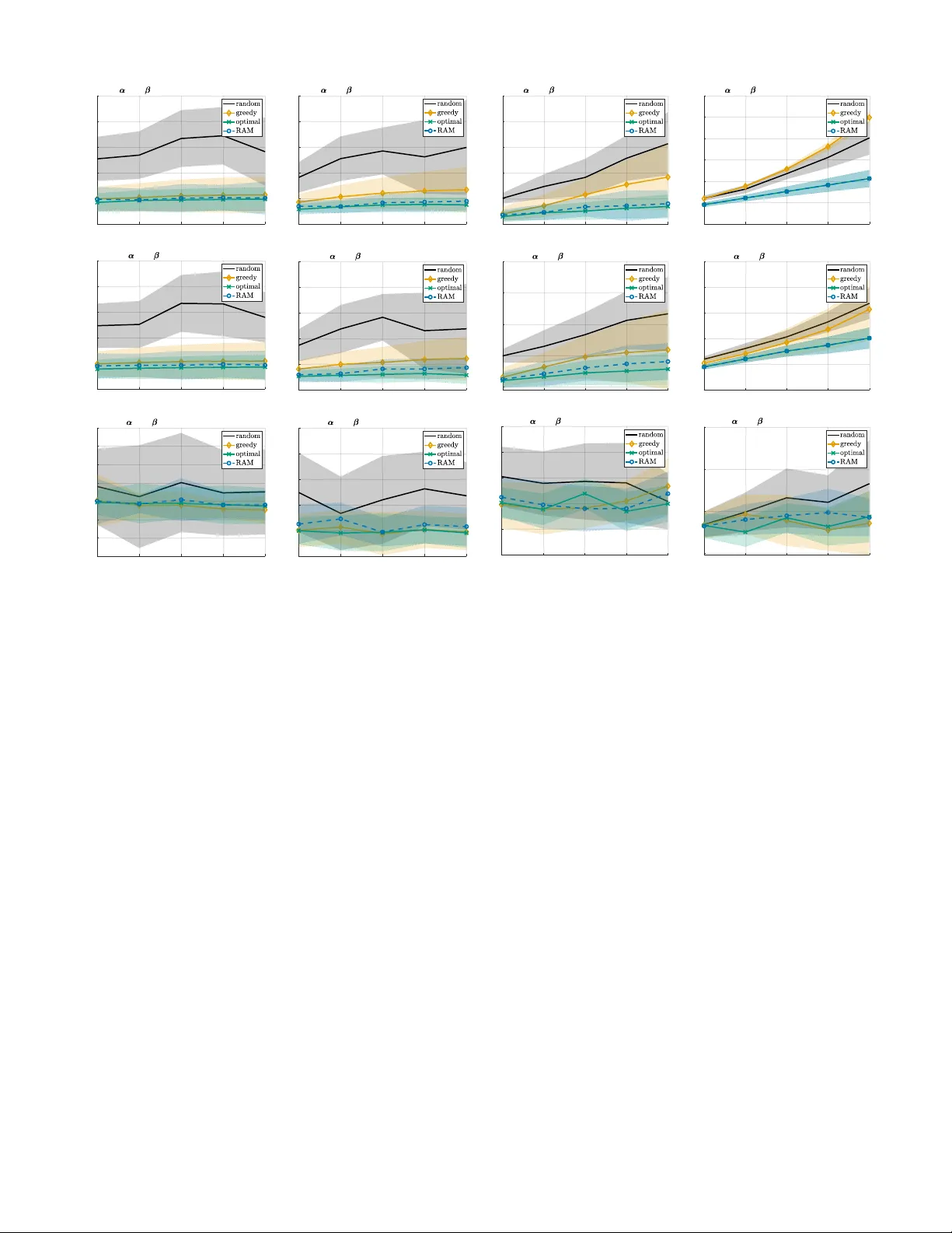
Rob ust and Adapti v e Sequential Submodular Optimization V asileios Tzoumas, ? Member , IEEE, Ali Jadbabaie, † F ellow , IEEE, George J. P appas, ‡ F ellow , IEEE. Abstract —Emerging applications of control, estimation, and machine learning, from target tracking to decentralized model ﬁtting, pose resour ce constraints that limit which of the available sensors, actuators, or data can be simultaneously used across time. Theref ore, many resear chers hav e proposed solutions within discrete optimization frameworks where the optimization is performed over ﬁnite sets. By exploiting notions of discr ete con- vexity , such as submodularity , the resear chers hav e been able to pro vide scalable algorithms with prov able suboptimality bounds. In this paper , we consider such problems b ut in adversarial en vironments, where in every step a number of the chosen elements in the optimization is remov ed due to failures/attacks. Speciﬁcally , we consider for the ﬁrst time a sequential version of the problem that allows us to observe the failures and adapt, while the attacker also adapts to our response. W e call the novel pr oblem Robust Sequential submodular Maximization ( RSM ). Generally , the problem is computationally hard and no scalable algorithm is known for its solution. Howe ver , in this paper we propose Robust and Adaptive Maximization ( RAM ), the ﬁrst scal- able algorithm. RAM runs in an online fashion, adapting in every step to the history of failur es. Also, it guarantees a near -optimal performance, even against any number of failures among the used elements. Particularly , RAM has both provable per -instance a priori bounds and tight and/or optimal a posteriori bounds. Finally , we demonstrate RAM ’ s near -optimality in simulations across various application scenarios, along with its robustness against several failure types, from worst-case to random. I . I N T RO D U C T I O N Control, estimation, and machine learning applications of the Internet of Things (IoT) and autonomous robots [1] require the sequential optimization of systems in scenarios such as: • Sensor scheduling: An unmanned aerial v ehicle (U A V) is assisted for its navig ation by on-board and on-ground sen- sors. Ideally , the U A V would use all a vailable sensors for nav- igation. Howe ver , limited on-board capacity for measurement- processing necessitates a sequential sensor scheduling prob- lem [2]: at each time step, which few sensors should be used for the U A V to effecti vely navig ate itself? • T ar get tracking: A wireless sensor network (WSN) is designated to monitor a mobile target. Limited battery power necessitates a sequential sensor activ ation problem [3]: at each time step, which few sensors should be acti v ated for the WSN to ef fectively track the target? ? Department of Aerospace Engineering, University of Michigan, Ann Arbor , MI 48109, USA. At the time the paper was accepted for publication: Laboratory for Information and Decision Systems, Massachusetts Institute of T echnology , Cambridge, MA 02139, USA. vtzoumas@umich.edu † Institute for Data, Systems and Society , Massachusetts Institute of T ech- nology , Cambridge, MA 02139 USA. jadbabai@mit.edu ‡ Department of Electrical and Systems Engineering, University of Penn- sylvania, Philadelphia, P A 19104 USA. pappasg@seas.upenn.edu The work was supported by the AFOSR Complex Networks program, and by the ARL CRA DCIST W911NF-17-2-0181 program. • Decentralized model ﬁtting: A team of mobile robots collects data to learn the model of an unknown environmental process. The data are transmitted to a fusion center , performing the statistical analysis. Ideally , all robots would transmit their data to the center at the same time. But instead, communication bandwidth constraints necessitate a sequential transmission problem [4]: at each time step, which fe w robots should trans- mit their data for the center to ef fectively learn the model? Similar applications of sensor and data scheduling, b ut also of actuator scheduling as well as infrastructure design are studied in [5]–[16]. P articularly , all applications abo ve require the sequential selection of a few elements, among a ﬁnite set of av ailable ones, to optimize performance across multiple steps subject to resource constraints. For example, the target tracking application above requires the sequential acti vation of a few sensors across the WSN, to optimize an estimation error subject to power constraints. Importantly , the activ ated sensors may vary in time, since each sensor may measure different parts of the target’ s state (e.g., some sensors may measure only position, others only speed). F ormally , all abov e applications moti vate the sequential optimization problem 1 max A 1 ⊆V 1 · · · max A T ⊆V T f ( A 1 , . . . , A T ) , s.t. |A t | = α t , t = 1 , . . . , T , (1) where T is a gi ven horizon; V t is a giv en ﬁnite set of av ailable elements to choose from at t such that V t ∩ V t 0 = ∅ for all t, t 0 = 1 , . . . , T ; 2 f : 2 V 1 ∪ · · · ∪ 2 V T 7→ R is a given objective function; α t is a given cardinality constraint, capturing the resource constraints at t ; and A t are the chosen elements at t , resulting from the solution of eq. (1). Notably , in all abov e applications, and [5]–[16], f is non-decreasing, and without loss of generality one may consider f ( ∅ ) = 0 . For example, in [11], f is the trace of the inv erse of the controllability Gramian, which captures the a verage control ef fort for dri ving the system; and in [8], f is the logdet of the error cov ariance of the minimum mean square batch-state estimator . Speciﬁcally , in [8], f is also submodular, a diminishing returns property that captures the intuition that a sensor’ s contribution to f ’ s value diminishes when more sensors are activ ated already . 1 Calligraphic fonts denote ﬁnite discrete sets (e.g., A ). 2 A denotes A ’ s power set. |A| its cardinality . A \ B denotes set difference: the elements in A not in B . Gi ven a set function f : 2 V 1 ∪ · · · ∪ 2 V T 7→ R , and A 1 ⊆ V 1 , . . . , A t ⊆ V t , for some positive integer t ≤ T , the f ( A 1 , . . . , A t ) denotes f ( A 1 ∪ · · · ∪ A t ∪ ∅ ∪ · · · ∪ ∅ ) where the ∅ is repeated T − t times, and ∅ denotes the empty set. R denotes the set of real numbers. 2 Even if the elements in V 1 , . . . , V T correspond to the same system modules, e.g., sensors, the elements among different V t are differentiated because they are chosen at different times. For example, consider the case where T = 2 , and two sensors s 1 and s 2 are av ailable to be chosen at each t ; then, by denoting with s i,t that sensor i is available to be chosen at t , it is V 1 = { s 1 , 1 , s 2 , 1 } and V 2 = { s 1 , 2 , s 2 , 2 } , and, naturally , V 1 ∩ V 2 = ∅ . Although the problem in eq. (1) is computationally hard, ef- ﬁcient algorithms hav e been proposed for its solution: when f is monotone and submodular, then eq. (1) is NP-hard [17] and the greedy algorithm in [18, Section 4] guarantees a constant suboptimality bound across all problem instances; and when f is only monotone, then eq. (1) is inapproximable (no polynomial time algorithm guarantees a constant bound across all instances) [19], [20] but the greedy algorithm in [18] guarantees per-instance bounds instead [21]–[23]. In this paper , ho wever , we shift focus to a nov el reformu- lation of eq. (1) that is robust against failures/attacks. Particu- larly , in all abo ve applications, at any time t , actuators can be cyber-attack ed [24], sensors can malfunction [25], and communication channels can be blocked [4], all resulting to denial-of-service (DoS) failures, in the sense that the actuators, sensors, channels, etc. will shut down (stop working), at least temporarily . Hence, in such failure-prone and adversarial scenarios, eq. (1) may fail to protect any of the above appli- cations, since it ignores the possibility of DoS failures. Thus, tow ards guaranteed protection, a rob ust reformulation becomes necessary that can both adapt to the history of incured failur es and account for futur e ones . Therefore, in this paper we introduce a novel rob ust op- timization framew ork, named Robust Sequential submodular Maximization ( RSM ), that goes beyond the failure-free eq. (1) and accounts for DoS failures/attacks. Speciﬁcally , we deﬁne RSM as the follo wing robust reformulation of eq. (1): RSM problem: max A 1 ⊆V 1 min B 1 ⊆A 1 · · · max A T ⊆V T min B T ⊆A T f ( A 1 \ B 1 , . . . , A T \ B T ) , s.t. |A t | = α t , |B t | ≤ β t , t = 1 , . . . , T . (2) where β t is a gi ven number of possible failures (generally , β t ∈ [0 , α t ] ); and B t is the failure against A t . By solving RSM , our goal is to maximize f despite worst- case failures that occur at each maximization step, as captured by the intermediate/subsequent minimization steps. Evidently , since RSM considers w orst-case failures, it is suitable when there is no prior on the f ailure mechanism, or when protection against worst-case failures is essential, such as in safety-cri- tical target tracking and costly experiment designs. RSM can be interpreted as a T -stage perfect information sequential game between a “maximization” player (defender) and a “minimization” player (attacker) [26, Chapter 4]. The defender starts the game and the players act sequentially , having perfect knowledge of each others’ actions: at each t , the defender selects an A t , and then the attacker responds with a worst-case remov al B t from A t , while both players account for the history of all actions up to t − 1 . In this context, the defender ﬁnds an optimal sequence A 1 , . . . , A T by accounting at each t (i) for the history of responses B 1 , . . . , B t − 1 , (ii) for the subsequent response B t , and (iii) for all remaining future responses B t +1 , . . . , B T . This is an additional computational challenge in comparison to the failure-free eq. (1), which is already computationally hard. No scalable algorithms exists for RSM . In this paper , to pr ovide the ﬁrst scalable algorithm, we develop an adaptive algorithm that at each t accounts only (i) for the history of responses up to t − 1 and (ii) for the subsequent response B t (but not for the remaining future responses up to t = T ), and as a result is scalable, but which still can guarantee a performance close to the optimal. Related work in combinatorial optimization. The ma- jority of the related work has focused on the failure-free eq. (1), when f is either monotone and submodular or only monotone. In more detail, Fisher et al. [18] focused on f being monotone and submodular , and proposed ofﬂine and online greedy algorithms that both guarantee the constant 1 / 2 suboptimality bound. Similarly , Conforti and Cornuéjols [27], Iyer et al. [28], and Sviridenko et al. [23] focused again on f being monotone and sumodular but provided instead per - instance, curvature-depended bounds. The bounds generally tighten the ones in [18]. Finally , Krause et al. [29], Das and Kempe [21], W ang et al. [22], and Sviridenko et al. [23] (see also the earlier [30]) focused on f being only monotone, and prov ed per-instance, curvature-depended bounds for the greedy algorithms in [18], using notions of curv ature —also referred to as “submodularity ratio”— they introduced. Recent work has also studied failure-rob ust reformulations of eq. (1), typically per RSM ’ s framew ork but only for T = 1 , wher e no adaptiveness is r equired . Speciﬁcally , when f is monotone and submodular , Orlin et al. [31] and Boguno vic et al. [32] provided greedy algorithms with constant sub- optimality bounds. Howe ver , the algorithms are valid only for limited numbers of f ailures (for β 1 ≤ √ α 1 in [31] and β 1 ≤ α 1 / (log α 1 ) 3 in [32]). In contrast, Tzoumas et al. [33] provided a greedy algorithm with per-instance bounds for any number of failures ( β 1 can take any value in [0 , α 1 ] ). Also, Rahmattalabi et al. [34] dev eloped a mixed-integer linear program approach for a locations monitoring problem. More recently , Tzoumas et al. [35] and Bogunovic et al. [36] extended the previous works on the T = 1 case by focusing on f being only monotone, and proved per -instance, curvature- dependent bounds for the algorithm introduced in [33]. In more detail, Bogunovic et al. [36] focuses on cardinality constraints, whereas Tzoumas et al. [35] on the more general matroid constraints, b ut, still, for the case where T = 1 . The latter framew ork enabled applications of failure-robust multi- robot robot planning, and particularly of acti ve information gathering [37] and target tracking [38]. Other relev ant work is that of Mitro vic et al. [39], where a memoryless failure- robust reformulation of eq. (1) is considered, instead of the sequential framework of RSM , which takes into account the history of past selections/failures. Finally , Mirzasoleiman et al. [40] and Kazemi et al. [41] adopted a robust optimization framew ork against non w orst-case failures, in contrast to RSM which is against worst-case failures. All in all, in comparison to all prior research, in this paper we analyze RSM ’ s multistep case T > 1 for the ﬁrst time, and consider adapti ve algorithms. Related work in control. In the robust/secure control literature, various approaches have been proposed to wards fault-tolerant control, secure control, as well as secure state estimation, against random failures, data injection and DoS failures/attacks [42]–[61]. In contrast to RSM ’ s resource- constrained framework, [42]–[61] focus in resource abundant en vironments where all sensors and actuators stay always activ e under normal operation. For example, [59]–[61] focus on DoS failures/attacks from the perspecti ve of packet loss and intermittent network connectivity , which can result to system destabilization. Generally , [42]–[61] focus on failure/attack detection and identiﬁcation, and/or secure estimator/controller design, instead of the adaptive activation of a few sensors/ac- tuators against worst-case DoS failur es/attacks per RSM . Contributions. W e introduce the novel RSM problem of robust sequential maximization against DoS failures/attacks. W e de velop the ﬁrst scalable algorithm, named Robust and Adaptive Maximization ( RAM ), that has the properties: • Adaptiveness: At each time t = 1 , 2 , . . . , RAM selects a robust solution A t in an online fashion, accounting for the history of failures B 1 , . . . , B t − 1 and of actions A 1 , . . . , A t − 1 , as well as, for all possible failures at t from A t . • System-wide r obustness: RAM is v alid for any number of failures; that is, for any β t ∈ [0 , α t ] , t = 1 , 2 , . . . . • P olynomial running time: RAM has the same order of running time as the polynomial time greedy algorithm proposed in [18, Section 4] for the failure-free eq. (1). • Pr ovable appr oximation performance: RAM has prov- able per-instance suboptimality bounds that quantify RAM ’ s near-optimality at each problem instance at hand. 3 Particu- larly , we provide both a priori and a posteriori per-instance bounds. The a priori bounds quantify RAM ’ s near -optimality before RAM has run. In contrast, the a posteriori bounds are computable online (as RAM runs), once the failures at each current step have been observed. The a posteriori bounds are tight and/or optimal. 4 Finally , we present approximations of the a posteriori bounds that are computable before each failure occurs. T o quantify the bounds, we use curvature notions by Conforti and Conruéjols [27], for monotone and submodular functions, and Sviridenko et al. [23], for monotone functions. W e demonstrate RAM ’ s effecti veness in applications of sen- sor scheduling, and of target tracking with wireless sensor networks. W e present a Monte Carlo analysis, where we vary the failure types from w orst-case to greedily and randomly selected failures, and compare RAM against a brute-force optimal algorithm (viable only for small-scale instances), the greedy algorithm in [18], and a random algorithm. In the results, we observe RAM ’ s near-optimality against worst-case failures, its robustness against non worst-case failures, and its superior performance against the compared algorithms. Comparison with the preliminary results in [62], which coincides with preprint [63]: This paper extents the results in [62], considers new simulations, and includes the proofs that were all omitted from [62]. Particularly , most of the technical results herein, including Theorem 13, Theorem 14, Corollary 21, and Algorithm 3, are novel and ha ve not been 3 Similarly to eq. (1), RSM is generally inapproximable: no polynomial time algorithm guarantees a constant suboptimality bound across all problem instances. For example, it is inapproximable for fundamental applications in control and machine learning such as sensor selection for optimal Kalman ﬁltering [20], and featur e selection for sparse model ﬁtting [19]. Thus, in this paper we focus our analysis in per -instance suboptimality bounds. 4 A suboptimality bound is called optimal when it is the tightest achiev able bound among all polynomial time algorithms, given a worst-case family of f . Algorithm 1: Robust adaptiv e maximization ( RAM ). Input: RAM receiv es the inputs: • Ofﬂine : integer T ; function f : 2 V 1 ∪ · · · ∪ 2 V T 7→ R such that f is non-decreasing and f ( ∅ ) = 0 ; integers α t , β t such that 0 ≤ β t ≤ α t ≤ |V t | , for all t = 1 , . . . , T ; • Online : at each t = 2 , . . . , T , observed remov al B t − 1 from RAM ’ s output A t − 1 . Output: At each step t = 1 , . . . , T , set A t . 1: for all t = 1 , . . . , T do 2: S t, 1 ← ∅ ; S t, 2 ← ∅ ; 3: Sort elements in V t s.t. V t ≡ { v t, 1 , . . . , v t, |V t | } and f ( v t, 1 ) ≥ . . . ≥ f ( v t, |V t | ) ; 4: S t, 1 ← { v t, 1 , . . . , v t,β t } ; 5: while |S t, 2 | < α t − β t do 6: x ∈ arg max y ∈V t \ ( S t, 1 ∪S t, 2 ) f ( A 1 \ B 1 , . . . , A t − 1 \ B t − 1 , S t, 2 ∪ { y } ) ; 7: S t, 2 ← { x } ∪ S t, 2 ; 8: end while 9: A t ← S t, 1 ∪ S t, 2 . 10: end for previously published. Also, the simulation scenarios are new and include a sensitivity analysis of RAM against v arious failure types (in [62] we tested RAM only against worst-case failures, and in different scenarios). Finally , all proofs in [62] were omitted and are no w included here. Organization of the rest of the paper . Section II presents RAM , and quantiﬁes its minimal running time. Section III presents RAM ’ s suboptimality bounds. Section IV presents RAM ’ s numerical ev aluations. Section V concludes the paper . All proofs are found in the appendix. I I . A N A DA P T I V E A L G O R I T H M : RAM W e present RAM , the ﬁrst scalable algorithm for RSM , for- mulated in eq. (2). RAM ’ s pseudo-code is given in Algorithm 1. Below , we ﬁrst gi ve an intuiti ve description of RAM , and then a step-by-step description. Also, we quantify its running time. RAM ’ s suboptimality bounds are given in Section III. A. Intuitive description RSM aims to maximize f through a sequence of steps despite compromises to each step. Speciﬁcally , at each t = 1 , 2 , . . . , RSM selects an A t tow ards a maximal f despite the fact that A t will be compromised by a worst-case remov al B t , resulting to f being ev aluated at A 1 \ B 1 , . . . , A T \ B T instead of A 1 , . . . , A T . In this context, RAM aims to achieve RSM ’ s goal by selecting A t as the union of two sets S t, 1 , and S t, 2 ( RAM ’ s line 9), whose role we describe intuiti vely below: a) S t, 1 appr oximates (aims to guess the) worst-case r emoval fr om A t : With S t, 1 , RAM aims to capture the worst- case remov al of β t elements from A t . Intuitiv ely , S t, 1 is aimed to act as a “bait” to a worst-case attacker that selects the best β t elements to remove from A t at time t ( best with respect to their contribution to wards RSM ’ s goal). RAM aims to approximate them by letting S t, 1 be the set of β t elements with the largest marginal contributions to f ( RAM ’ s lines 3- 4). As such, each S t, 1 is independent of the history of actual remov als B 1 , . . . , B t − 1 and can be computed of ﬂine, before any of the B 1 , . . . , B T has been realized. In contrast, S t, 2 can only be computed online, as we describe belo w . b) S t, 1 ∪ S t, 2 appr oximates optimal solution to RSM ’ s t - th step: T o complete A t ’ s construction, RAM needs to select a set S t, 2 of α t − β t elements (since |A t | = α t and |S t, 1 | = β t ), and return A t = S t, 1 ∪ S t, 2 ( RAM ’ s line 9). Assuming S t, 1 ’ s remov al from A t , for A t to be an optimal solution to RSM ’ s t -th maximization step, RAM needs to select S t, 2 as a best set of α t − β t elements from V t \ S t, 1 . Nev ertheless, this problem is NP-hard [17]. Thereby , RAM approximates such a best set, using the greedy procedure in RAM ’ s lines 5-8. Particularly , RAM ’ s line 6 adapts S t, 2 to the history of remov als B 1 , . . . , B t − 1 and selections A 1 , . . . , A t − 1 , since it constructs S t, 2 giv en A 1 \ B 1 , . . . , A t − 1 \ B t − 1 . As such, each S t, 2 , in contrast to S t, 1 , can be computed only online, only once the history of remov als B 1 , . . . , B t − 1 has been realized. Overall, RAM adaptiv ely constructs an A t to approximate an optimal solution to RSM ’ s t -th maximization step. Remark 1 (Further intuition on wh y S t, 1 and S t, 2 are selected as in RAM ) . W e ﬁr st discuss why RAM (i) selects A t as the union of S t, 1 and S t, 2 , and (ii) selects S t, 2 as a gr eedily picked subset of V t \ S t, 1 . W e then focus on S t, 1 . If S t, 1 guesses correctly the r emoval B t fr om A t = S t, 1 ∪ S t, 2 , then all elements in S t, 2 r emain intact ( A t \ B t = S t, 2 ) . Ther efor e, since S t, 2 has been selected using the gr eedy algorithm in RAM ’ s lines 5-8, whic h is an optimal appr oxima- tion algorithm for maximizing monotone functions subject to car dinality constraints [23], 5 A t is an optimal appr oximation to RSM ’s t -th maximization step. This explains why RAM selects A t as the union of two sets ( S t, 1 and S t, 2 ), and why RAM selects S t, 2 gr eedily fr om V t \ S t, 1 given S t, 1 . Generally , if S 1 , 1 , . . . , S T , 1 guess B 1 , . . . , B T corr ectly , then RSM becomes equivalent to the attack-fr ee eq. (1) , and RAM becomes equivalent to the optimal gr eedy algorithm for eq. (1) . But if S t, 1 guesses incorrectly B t , then some of S t, 1 ’ s elements will survive, and, instead, some of S t, 2 ’ s elements will be remo ved. The question arising now is: Can the elements that survived in S t, 1 compensate for the r emoved elements fr om S t, 2 ? In this paper , we develop tools to pr ove that if the elements of S t, 1 ar e chosen as in RAM ’ s lines 3-4, this is indeed the case (pr oof of Theorem 10), pr oviding the ﬁrst pr ovable approximation guarantees for RSM via RAM . B. Step-by-step description RAM ex ecutes four steps for each t = 1 , . . . , T : a) Initialization ( RAM ’ s line 2): RAM deﬁnes two auxil- iary sets, namely , S t, 1 and S t, 2 , and initializes them with the empty set ( RAM ’ s line 2). b) Construction of set S t, 1 ( RAM ’ s lines 3-4): RAM con- structs S t, 1 by selecting β t elements, among all s ∈ V t , with the highest values f ( s ) . In detail, S t, 1 is constructed by ﬁrst 5 An approximation algorithm is called optimal when it achiev es the tightest possible achiev able suboptimality bound among all polynomial time algorithms, given a worst-case family of functions f . indexing the elements in V t such that V t ≡ { v t, 1 , . . . , v t, |V t | } and f ( v t, 1 ) ≥ . . . ≥ f ( v t, |V t | ) ( RAM ’ s line 3), and then by including in S t, 1 the ﬁst β t elements ( RAM ’ s line 4). c) Construction of set S t, 2 ( RAM ’ s lines 5-8): RAM constructs S t, 2 by picking greedily α t − β t elements from V t \ S t, 1 , taking also into account the history of selections and removals, that is, A 1 \ B 1 , . . . , A t − 1 \ B t − 1 . Speciﬁcally , the “while loop” ( RAM ’ s lines 5-8) selects an element y ∈ V t \ ( S t, 1 ∪ S t, 2 ) to add in S t, 2 only if y maximizes the value of f ( A 1 \ B 1 , . . . , A t − 1 \ B t − 1 , S t, 2 ∪ { y } ) . d) Construction of set A t ( RAM ’ s line 9): RAM constructs A t as the union of S t, 1 and S t, 2 . The abov e steps are valid for any number of failures β t . C. Running time W e now analyze the computational complexity of RAM . Proposition 2. At each t = 1 , 2 , . . . , RAM runs in O [ |V t | ( α t − β t ) τ f ] time, where τ f is f ’ s evaluation time. Remark 3 (Minimal running time) . Even though RAM r o- bustiﬁes the traditional, failure-fr ee sequential optimization in eq. (1) , RAM has the same or der of running time as the state-of- the-art algorithms for eq. (1) [18, Section 4] [23, Section 8]. In summary , RAM selects adaptiv ely a solution for RSM , in minimal running time, and is valid for an y number of failures. W e quantify its approximation performance next. I I I . S U B O P T I M A L I T Y G U A R A N T E E S W e present RAM ’ s suboptimality bounds. W e ﬁrst present RAM ’ s a priori bounds, and, then, the a posteriori bounds. Finally , we present the latter’ s pre-failure approximations. A. Curvatur e and total curvature T o present RAM ’ s suboptimality bounds we use the notions of curvature and total curvature . T o this end, we start by recalling the deﬁnitions of modularity and submodularity , where we consider the notation: • V , S T i =1 V t ; i.e., V is the union across the horizon T of all the av ailable elements to choose from; Deﬁnition 4 (Modularity [64]) . f : 2 V 7→ R is modular if and only if f ( A ) = P v ∈A f ( v ) , for any A ⊆ V . Therefore, if f is modular , then V ’ s elements complement each other through f . Particularly , Deﬁnition 4 implies f ( { v }∪ A ) − f ( A ) = f ( v ) , for any A ⊆ V and v ∈ V \ A . Deﬁnition 5 (Submodularity [64]) . f : 2 V 7→ R is submodular if and only if f ( A ∪ { v } ) − f ( A ) ≥ f ( B ∪ { v } ) − f ( B ) , for any A ⊆ B ⊆ V and v ∈ V . The deﬁnition implies f is submodular if and only if the return f ( A ∪ { v } ) − f ( A ) diminishes as A grows, for an y v . In contrast to f being modular, if f is submodular , then V ’ s elements substitute each other . Speciﬁcally , without loss of generality , consider f to be non-negati ve: then, Deﬁnition 5 implies f ( { v } ∪ A ) − f ( A ) ≤ f ( v ) . That is, in the presence of A , v ’ s contribution to f ( { v } ∪ A ) ’ s v alue is diminished. Algorithm 2: Online greedy algorithm [18, Section 4]. Input: Integer T > 0 ; f : 2 K 1 ∪ · · · ∪ 2 K T 7→ R such that f is non-decreasing and f ( ∅ ) = 0 ; integers δ t such that 0 ≤ δ t ≤ |K t | , for all t = 1 , . . . , T . Output: At each step t = 1 , . . . , T , set M t . 1: for all t = 1 , . . . , T do 2: M t ← ∅ ; 3: while |M t | < δ t do 4: x ∈ arg max y ∈K t \M t f ( M 1 , . . . , M t − 1 , M t ∪ { y } ) ; 5: M t ← { x } ∪ M t ; 6: end while 7: end for Deﬁnition 6. (Curv ature [27]) Consider a non-decr easing submodular f : 2 V 7→ R such that f ( v ) 6 = 0 , for any v ∈ V , without loss of gener ality . Then, f ’ s curvature is deﬁned as κ f , 1 − min v ∈V f ( V ) − f ( V \ { v } ) f ( v ) . (3) Deﬁnition 6 implies κ f ∈ [0 , 1] . Particularly , κ f measures how far f is from modularity: if κ f = 0 , then f ( V ) − f ( V \ { v } ) = f ( v ) , for all v ∈ V ; that is, f is modular . In contrast, if κ f = 1 , then there exist v ∈ V such that f ( V ) = f ( V \ { v } ) ; that is, v has no contrib ution to f ( V ) in the presence of V \ { v } . Therefore, κ f can also been interpreted as a measure of how much V ’ s elements complement/substitute each other . Deﬁnition 7 (T otal curvature [23], [30]) . Consider a monotone f : 2 V 7→ R . Then, f ’ s total curvatur e is deﬁned as c f , 1 − min v ∈V min A , B⊆V \{ v } f ( { v } ∪ A ) − f ( A ) f ( { v } ∪ B ) − f ( B ) . (4) Similarly to κ f , it also is c f ∈ [0 , 1] . Remarkably , when f is submodular, then c f = κ f . Generally , if c f = 0 , then f is modular , while if c f = 1 , then eq. (4) implies the assumption that f is non-decreasing. In [65], any monotone f with total curvature c f is called c f -submodular , as repeated below . 6 Deﬁnition 8 ( c f -submodularity [65]) . Any monotone function f : 2 V 7→ R with total curvatur e c f is called c f -submodular . Remark 9 (Dependence on the size of V and length of horizon T ) . Evidently , both κ f and c f ar e non-decr easing as V gr ows (cf. Deﬁnition 6 and Deﬁnition 7). Ther efor e, κ f and c f ar e also non-decr easing as T incr eases, since V ≡ S T i =1 V t . B. A priori suboptimality bounds W e present RAM ’ s a priori suboptimality bounds, using the abov e notions of curvature. W e use also the notation: • f ? is the optimal v alue of RSM ; • A 1: t , ( A 1 , . . . , A t ) , where A t is the selected set by RAM at t = 1 , 2 , . . . ; 6 Lehmann et al. [65] deﬁned c f -submodularity by considering in eq. (4) A ⊆ B instead of A ⊆ V . Generally , non submodular but monotone functions hav e been referred to as appr oximately or weakly submodular [29], [66], names that ha ve also been adopted for the deﬁnition of c f in [65], e.g., in [67], [68]. • ( B ? 1 , . . . , B ? T ) is an optimal remov al from A 1: T ; • B ? 1: t , ( B ? 1 , . . . , B ? t ) ; • A 1: t \ B ? 1: t , ( A 1 \ B ? 1 , . . . , A t \ B ? t ) . Theorem 10 (A priori bounds) . RAM selects A 1: T such that |A t | ≤ α t , and if f is submodular , then f ( A 1: T \ B ? 1: T ) f ? ≥ ( 1 − e − κ f κ f (1 − κ f ) , T = 1; (1 − κ f ) 4 , T > 1; (5) wher eas, if f is c f -submodular , then f ( A 1: T \ B ? 1: T ) f ? ≥  (1 − c f ) 3 , T = 1; (1 − c f ) 5 , T > 1 . (6) Evidently , Theorem 10’ s bounds are a priori, since in- eqs. (5)’ s and (6)’ s right-hand-sides are independent of the selected A 1: T by RAM , and the incurred failures B ? 1: T . Importantly , the bounds compare RAM ’ s selection A 1: T against an optimal one that knows a priori all future failures (and achiev es that way the value f ? ). Instead, RAM ’ s has no kno wledge of the future failures. W ithin this challenging setting, Theorem 10 nonetheless implies: for functions f with κ f < 1 or c f < 1 , RAM ’ s selection A 1: T is ﬁnitely close to the optimal, instead of arbitrarily suboptimal. Indeed, then Theorem 10’ s bounds are non-zero. W e discuss functions with κ f < 1 or c f < 1 below , along with rele vant applications. Remark 11 (Functions with κ f < 1 , c f < 1 , and applica- tions) . Functions with κ f < 1 are the concave over modular functions [28, Section 2.1] and the log det of positive-deﬁnite matrices [69]. Also, functions with c f < 1 are the support selection functions [66], the aver age minimum squar e err or of the Kalman ﬁlter (trace of err or covariance) [70, Section IV], and the LQG cost as a function of the active sensor s [10, The- or em 4]. The aforementioned functions appear in control and machine learning applications such as featur e selection [21], [71], and actuator and sensor scheduling [5]–[13], [70]. Evidently , when κ f and c f tend to 0, then RAM becomes optimal, since all bounds in Theorem 10 tend to 1 ; for example, 1 /κ f (1 − e − κ f )(1 − κ f ) increases as κ f decreases, and its limit is equal to 1 for κ f → 0 . Application examples of this sort in volv e the regression of Gaussian processes with RBF kernels [69, Theorem 5], such as in sensor selection for temperature monitoring [72]. Finally , since both κ f and c f are non-decreasing in T and V (Remark 9), the bounds are non-increasing in T and V . T ightness and optimality (towar ds a posteriori bounds): RAM ’ s curvature-dependent bounds are the ﬁrst suboptimality bounds for RSM , and make a ﬁrst step towards separating the classes of monotone functions into functions for which RSM can be approximated well (low curvature functions), and functions for which it cannot (high curvature functions). Moreov er , although for the failure-free eq. (1) the a priori bounds 1 /κ f (1 − e − κ f ) and 1 / (1 + κ f ) (where f is submod- ular) are known to be tight [27, Theorem 2.12, Theorem 5.4], the tightness of ineq. (5) is an open problem. Similarly , although for eq. (1) the a priori bound 1 − c f (where f is c f -submodular) is kno wn to be optimal (the tightest possible in polynomial time in a worst-case) [23, Theorem 8.6], the optimality of ineq. (6) is an open problem. Notably , in the latter case ( f is c f -submodular) both 1 − c f and the bound in ineq. (6) are 0 for c f = 1 , which is in agreement with the inapproximability of both eq. (1) and RSM in the worst-case. In contrast to Theorem 10’ s a priori bounds, we next present tight and/or optimal a posteriori bounds. C. A posteriori suboptimality bounds W e now present RAM ’ s a posteriori bounds, which are computable once all failures up to step t hav e been observed. Henceforth, we use the notation: • f ? t is the optimal v alue of RSM for T = t ; • M t is the set returned by the online, failure-free greedy Algorithm 2 at t = 1 , . . . , T , 7 when we consider therein δ t = α t − β t and K t = V t \ S 1 ,t ; • M 1: t , {M 1 , . . . , M t } . Remark 12 (Interpretation of M 1: t ) . Since each S 1 ,t is the expected futur e failures (“baits”) selected in RAM ’s lines 3-4 (see Section II), M 1: t ar e the sets one would greedily select per Algorithm 2 if it was known a priori that indeed the future failur es ar e the S 1 ,t , t = 1 , . . . , T . Theorem 13 (A posteriori bounds) . F or all t = 1 , . . . , T , given the observed history B ? 1: t , RAM selects A t such that |A t | ≤ α t , and if f is submodular , then f ( A 1: t \ B ? 1: t ) f ? t ≥ ( 1 − e − κ f κ f f ( A 1 \B ? 1 ) f ( M 1 ) , t = 1; 1 1+ κ f f ( A 1: t \B ? 1: t ) f ( M 1: t ) , t > 1; (7) wher eas, if f is c f -submodular , then f ( A 1: t \ B ? 1: t ) f ? t ≥ (1 − c f ) f ( A 1: t \ B ? 1: t ) f ( M 1: t ) . (8) Theorem 14 (Tightness and optimality) . There exist families of f such that the suboptimality bounds in ineq. (7) are tight. Also, ther e exist families of f suc h that the suboptimality bounds in eq. (8) are optimal (the tightest possible) acr oss all algorithms that e valuate f a polynomial number of times. 8 The bounds break down into the a priori κ f - and c f - depended parts, and the a posteriori f ( A 1: t \ B ? 1: t ) /f ( M 1: t ) . W e refer to the latter as a posteriori since it is computable after B ? t has been observed. Intuiti vely , the a posteriori part captures how successful the “bait” S 1 ,t has been in approximating the anticipated worst-case f ailure B ? t . Indeed, if B ? t = S 1 ,t for all t = 1 , 2 , . . . , then f ( A 1: t \ B ? 1: t ) /f ( M 1: t ) = 1 and Theorem 13’ s bounds become the tight/optimal a priori bounds 1 /κ f (1 − e − κ f ) , 1 / (1 + κ f ) and 1 − c f , 9 and, as such, they are also tighter than Theorem 10’ s a priori bounds. In general, Theorem 13’ s a posteriori bounds may be looser than Theorem 10’ s a priori bounds; yet, they are tighter when 7 W e refer to Algorithm 2 as “online” since each M t can be chosen in real time (at time t ) sequentially , i.e., given the history of past selections M 1 , . . . , M t − 1 . Observe, howev er, that if one wishes so one can also execute all steps of Algorithm 2 of ﬂine at time t = 0 . 8 Theorem 14’ s function families are the same as those in the proofs of [27, Theorem 2.12, Theorem 5.4] and [23, Theorem 8.6], which prove the tightness and optimality of 1 /κ f (1 − e − κ f ) , 1 / (1 + κ f ) and (1 − c f ) for eq. (1). 9 Theorem 14 is pro ved based on this observation. f ( A 1: t \ B ? 1: t ) /f ( M 1: t ) is close enough to 1: e.g., for f being c f -submodular and T > 1 , if f ( A 1: t \ B ? 1: t ) /f ( M 1: t ) > (1 − c f ) 4 , then the a posteriori bound in eq. (8) is tighter than the a priori in eq. (6). Indeed, in the numerical ev aluations of Section IV, f ( A 1: t \ B ? 1: t ) /f ( M 1: t ) is nearly 1, whereas (1 − c f ) 4 ≤ . 0001 ; thus, eq. (8) is 3 orders tighter than eq. (6). Notably , the a priori parts 1 /κ f (1 − e − κ f ) , 1 / (1 + κ f ) are non-zero for any values of κ f . In more detail, 1 /κ f (1 − e − κ f ) ≥ 1 − 1 /e and 1 / (1 + κ f ) ≥ 1 / 2 for all κ f ∈ [0 , 1] ; particularly , 1 /κ f (1 − e − κ f ) increases as κ f decreases, and its limit is equal to 1 for κ f → 0 . Therefore, in contrast to the a priori bound in eq. (5), which for κ f = 1 becomes 0, eq. (7) for κ f = 1 becomes instead f ( A 1: t \ B ? 1: t ) f ? t ≥ ( (1 − 1 /e ) f ( A 1 \B ? 1 ) f ( M 1 ) , t = 1; f ( A 1: t \B ? 1: t ) 2 f ( M 1: t ) , t > 1 . (9) Nev ertheless, such simpliﬁcation for eq. (8) is not evident, a fact that is in agreement with both (i) RSM ’ s inapproximability when f is not submodular , necessitating per-instance subop- timality bounds for any polynomial time algorithm, and (ii) eq. (8)’ s optimality per Theorem 14. Overall, Theorem 13’ s bounds are computable online, at each t = 1 , 2 , . . . , after f ailure B ? t has been observed. W e next approximate the bounds befor e B ? t occurs. D. Pr e-failure appr oximations of post-failur e bounds W e present pre-failure approximations to Theorem 13’ s post-failure bounds. In particular, we propose a method to lower bound f ( A 1: t \ B ? 1: t ) by a value ˆ f t , at each t = 1 , . . . , T , giv en B ? 1: t − 1 (but before B ? t occurs). In more detail, we recall f ( A 1: t \ B ? 1: t ) is the value of the constrained optimization problem f ( A 1: t \ B ? 1: t ) ≡ min B t ⊆A t , |B t |≤ β t f ( A 1: t − 1 \ B ? 1: t − 1 , A t \ B t ) . (10) Computing f ( A 1: t \ B ? 1: t ) is NP-hard, ev en if f is submodu- lar [73]. But lower bounding f ( A 1: t \ B ? 1: t ) can be efﬁcient. Speciﬁcally , the non-constrained reformulation of eq. (10) in eq. (11) belo w is efﬁciently solv able (see [73]–[76] for f being submodular; and [77] for f being c f -submodular): min B t ⊆A t f ( A 1: t − 1 \ B ? 1: t − 1 , A t \ B t ) + λ t |B t | , (11) where λ t ≥ 0 and constant ( λ t acts similarly to a Lagrange multiplier [78]). Evidently , Lemma 15 below holds true, where ˆ B t ( λ t ) denotes an optimal solution to eq. (11), i.e., ˆ B t ( λ t ) ∈ arg min B t ⊆A t f ( A 1: t − 1 \ B ? 1: t − 1 , A t \ B t ) + λ t |B t | , (12) and where ˆ f t ( λ t ) denotes the v alue of f ( A 1: t − 1 \ B ? 1: t − 1 , A t \ B t ) when B t = ˆ B t ( λ t ) , i.e., ˆ f t ( λ t ) , f ( A 1: t − 1 \ B ? 1: t − 1 , A t \ ˆ B t ( λ t )) . (13) Lemma 15. Ther e e xists λ ? t such that ˆ f t ( λ t ) ≤ f ( A 1: t \ B ? 1: t ) and | ˆ B t ( λ t ) | > β t for λ t < λ ? t ; wher eas, ˆ f t ( λ t ) ≥ f ( A 1: t \ B ? 1: t ) and | ˆ B t ( λ t ) | ≤ β t for λ t ≥ λ ? t . Algorithm 3: Bisection. Input: Integer β t per RSM ; function f per RSM ; histories A 1: t and B ? 1: t − 1 ; u 0 > 0 such that | ˆ B t ( u 0 ) | < β t , where ˆ B t ( · ) is deﬁned in eq. (12);  > 0 , which deﬁnes bise- ction’ s stopping condition (accuracy lev el). Output: λ t ≥ 0 such that ˆ f t ( λ t ) ≤ f ( A 1: t \ B ? 1: t ) , where λ t and ˆ f t ( λ t ) are deﬁned in eq. (11) and eq. (13). 1: l ← 0 ; u ← u 0 ; λ t ← ( l + u ) / 2 ; 2: while u − l >  do 3: Find ˆ B t ( λ t ) by solving eq. (12); 4: if | ˆ B t ( λ t ) | < β t then 5: u ← λ t ; { u always satisﬁes | ˆ B t ( u ) | < β t } 6: else 7: l ← λ t ; { l always satisﬁes | ˆ B t ( l ) | ≥ β t } 8: end if 9: λ t ← ( l + u ) / 2 ; 10: end while 11: λ t ← l ; { l is  -close to λ ? t ( λ ? t is deﬁned in Lemma 15) and satisﬁes | ˆ B t ( l ) | ≥ β t } 12: retur n λ t . T o observe such a value λ ? t exists, it sufﬁces to observe: (i) for λ t = 0 , the cardinality of ˆ B t in eq. (11) is unconstrained, and, thus, the optimal solution in eq. (11) is to remov e all A t , which implies | ˆ B t ( λ t ) | = α t ≥ β t ; (ii) more generally , for λ t > 0 , the cardinality of ˆ B t in eq. (11) is increasingly penalized as λ t increases, and, thus, | ˆ B t ( λ t ) | is a decreasing function of λ t (in particular, if λ t → + ∞ , then | ˆ B t ( λ t ) | → 0 ). Now , given (i)-(ii), denote by λ ? t the ﬁrst value of λ t such that | ˆ B t ( λ t ) | ≤ β t , when λ t is initially set to 0 and then continuously increases: then, for λ t < λ ? t , it is | ˆ B t ( λ t ) | > β t , and, thus, ˆ f t ( λ t ) ≤ f ( A 1: t \ B ? 1: t ) , since | ˆ B t ( λ t ) | > β t = |B ? t | and ˆ B t ( λ t ) is an optimal solution to eq. (11); whereas, for λ t ≥ λ ? t , it is | ˆ B t ( λ t ) | ≤ β t , and, thus, ˆ f t ( λ t ) ≥ f ( A 1: t \ B ? 1: t ) . Although λ ? t is unknown, it can be approximated by using bisection. For example, Algorithm 3 uses bisection with ac- curacy level  > 0 (Algorithm 3’ s lines 2-10) to ﬁnd a λ t that is  -close to λ ? t and for which ˆ f t ( λ t ) ≤ f ( A 1: t \ B ? 1: t ) . T o start the bisection, Algorithm 3 assumes a large enough u 0 ≥ 0 such that | ˆ B t ( u 0 ) | < β t ; such a u 0 can be found since | ˆ B t ( u 0 ) | → 0 for u 0 → + ∞ . Ne xt, at each “while loop” (lines 2-10 of Algorithm 3), λ ? t ∈ [ l , u ] , since | ˆ B t ( u ) | < β t and | ˆ B t ( l ) | ≥ β t (cf. line 5 and line 7 of Algorithm 3). Per line 2 of the algorithm, l and u are updated until u − l ≤  . Then, after at most log 2 [( u − l ) / ] iterations, the algorithm terminates by setting λ t equal to the latest value of l (lines 11- 12 of the algorithm). Therefore, λ t is  -close to λ ? t and satisﬁes | ˆ B t ( l ) | ≥ β t , which in turn implies ˆ f t ( λ t ) ≤ f ( A 1: t \ B ? 1: t ) , as desired. All in all, gi ven an approximation λ t to λ ? t , Lemma 15 implies the following approximation of Theorem 13’ s bounds. Corollary 16 (Pre-failure approximation of a posteriori bounds) . Let Algorithm 3 r eturn λ t , for t = 1 , . . . , T . RAM selects A t such that |A t | ≤ α t , and if f is submodular , then f ( A 1: t \ B ? 1: t ) f ? t ≥    1 − e − κ f κ f ˆ f 1 ( λ 1 ) f ( M 1 ) , t = 1; 1 1+ κ f ˆ f t ( λ t ) f ( M 1: t ) , t > 1; (14) wher eas if f is c f -submodular , then f ( A 1: t \ B ? 1: t ) f ? t ≥ (1 − c f ) ˆ f t ( λ t ) f ( M 1: t ) . (15) Corollary 16 describes an online mechanism to predict RAM ’ s performance before the upcoming failures, step by step. Remark 17 (Utility of Corollary 16’ s bounds) . F or T = 1 , Cor ollary 16’ s bounds are computed befor e B ? 1 occurs, which implies ˆ f 1 can be computed of ﬂine ( at any time t < 1 ) . Ther efor e, Cor ollary 16’ s bounds, when tighter than Theo- r em 10’s a priori bounds, allow for an a priori assessment of RAM ’s appr oximation performance (before RAM is deployed in the r eal world ) . Examples of 1-step design pr oblems wher e T = 1 , include robust actuator and sensor placement [7], [16], [79], robust feature selection [21], [32], [80], robust graph cov ering [81], and robust server placement [15], [82]. F or T > 1 , Corollary 16’ s bounds can only be computed online , once B ? 1: t − 1 has been observed (but befor e B ? t has occurr ed), for each t = 1 , . . . , T . 10 As such, the bounds can be used to balance the tr ade-off between (i) computation time r equir ements (including computation and energy consumption r equir ements) for solving eac h step t of RSM , and (ii) appr ox- imation performance requir ements for solving RSM at each t . F or example , if Cor ollary 16’s bounds indicate a good performance by RAM at t (e.g ., the bounds are above a given thr eshold), RAM is used to select A t , since RAM is computation time inexpensive , being a polynomial time algorithm. Howe ver , if the bounds indicate poor performance by RAM at t (less than the given thr eshold), then an optimal algorithm can be used instead at t (such as the one proposed in [34]), but at the expense of higher computation time, since any optimal algorithm is non-polynomial in the worst-case . 11 I V . A P P L I C A T I O N S W e e valuate RAM ’ s performance in applications. W e start by assessing its near-optimality against worst-case failures. W e continue by testing its sensitivity against non worst-case failures, particularly , random and greedily selected failures. For such failures, one would expect RAM ’ s performance to be the same, or improve, since RAM is designed to withstand the worst-case. T o these ends, we consider two applications from the introduction: sensor sc heduling for autonomous naviga- tion , and tar get trac king with wir eless sensor networks . 10 Corollary 16’ s bounds can only be computed online since RAM itself is an online algorithm, computing A t only once B ? 1: t − 1 has been observed (yet before B ? t has occurred), for each t = 1 , . . . , T . 11 Even when RAM is used in combination with another algorithm to choose A 1: t , Corollary 16’ s bounds are still applicable since they are algorithm agnostic (cf. proof of Theorem 13). 1 2 3 4 5 Time (t) 50 100 150 200 250 300 Error = 8; = 4; worst-case failure 1 2 3 4 5 Time (t) 100 200 300 400 500 600 Error = 8; = 5; worst-case failure 1 2 3 4 5 Time (t) 200 400 600 800 1000 1200 Error = 8; = 6; worst-case failure 1 2 3 4 5 Time (t) 0 500 1000 1500 2000 2500 3000 Error = 8; = 7; worst-case failure 1 2 3 4 5 Time (t) 50 100 150 200 250 300 Error = 8; = 4; greedy failure 1 2 3 4 5 Time (t) 100 200 300 400 500 600 Error = 8; = 5; greedy failure 1 2 3 4 5 Time (t) 200 400 600 800 1000 Error = 8; = 6; greedy failure 1 2 3 4 5 Time (t) 0 500 1000 1500 2000 2500 Error = 8; = 7; greedy failure 1 2 3 4 5 Time (t) -20 0 20 40 60 80 100 120 Error = 8; = 4; random failure 1 2 3 4 5 Time (t) 0 50 100 150 200 250 Error = 8; = 5; random failure 1 2 3 4 5 Time (t) -100 0 100 200 300 400 Error = 8; = 6; random failure 1 2 3 4 5 Time (t) 0 500 1000 1500 Error = 8; = 7; random failure Fig. 1. Representati ve simulation results for the application sensor scheduling for autonomous navigation . Results are av eraged across 100 Monte Carlo runs. Depicted is the estimation error for increasing time t , per eq. (16), where α t = α = 8 across all subﬁgures, whereas β t = β where β varies across subﬁgures column-wise. Finally , the failure type also varies, but row-wise. Each subﬁgur e has dif ferent scale. A. Sensor scheduling for autonomous navigation W e demonstrate RAM ’ s performance in autonomous na viga- tion scenarios, in the presence of sensing failures. W e focus on small-scale instances, to enable RAM ’ s comparison with a brute-force algorithm attaining the optimal to RSM . Instead, in Section IV -B we consider larger-scale instances. A U A V moves in a 3D space, starting from a randomly selected initial location. Its objective is to land at [0 , 0 , 0] with zero velocity . The U A V is modeled as a double-integrator with state x t = [ p t v t ] > ∈ R 6 , where t = 1 , 2 , . . . is the time index, p t is the U A V’ s position, and v t is its velocity . The U A V controls its acceleration. The process noise has co variance I 6 . The UA V is equipped with two on-board sensors: a GPS, measuring the U A V’ s position p t with a cov ariance 2 · I 3 , and an altimeter , measuring p t ’ s altitude component with standard deviation 0 . 5m . Also, the U A V can communicate with 10 linear ground sensors. These sensors are randomly generated at each Monte Carlo run, along with their noise cov ariance. The U A V has limited on-board battery po wer and measure- ment-processing bandwidth. Hence, it uses only a few sensors at each t . Particularly , among the 12 av ailable sensors, the U A V uses at most α , where α varies from 1 to 12 in the Monte Carlo analysis (per RSM ’ s notation, α t = α for all t = 1 , 2 , . . . ). The UA V selects the sensors to minimize the cumulativ e batch-state error over a horizon T = 5 , captured by c ( A 1: t ) = log det[Σ 1: t ( A 1: t )] , (16) where Σ 1: t ( A 1: t ) is the error covariance of the minimum variance estimator of ( x 1 , . . . , x t ) giv en the used sensors up to t [83]. Notably , f ( A 1: t ) = − c ( A 1: t ) is non-decreasing and submodular , in congruence to RSM ’ s framework [8]. Finally , we consider that at most β failures are possible at each t (per RSM ’ s notation, β t = β for all t ). In the Monte Carlo analysis, β varies from 0 to α − 1 . Baseline algorithms. W e compare RAM with three algo- rithms. The ﬁrst algorithm is a brute-force, optimal algorithm, denoted as optimal . Evidently , optimal is viable only for small- scale problem instances, such as herein where the av ailable sensors are 12. The second algorithm performs random selec- tion and is denoted as r andom . The third algorithm, denoted as greedy , greedily selects sensors to optimize eq. (16) per the failure-free optimization setup in eq. (1). Results. The results are av eraged over 100 Monte Carlo runs. F or α = 8 and β = 4 , 5 , 6 , 7 , the y are reported in Fig. 1. For the remaining α and β v alues, the qualitati ve results are the same. From Fig. 1, the follo wing observations are due: a) Near-optimality against wor st-case failur es: W e focus on Fig. 1’ s ﬁrst row of subﬁgures, where β varies from 4 to 7 (from left to right). Across all β , RAM nearly matches optimal . In contrast, greedy nearly matches optimal only for β = 4 (and, generally , for β ≤ α/ 2 , taking into account the simulation results for the remaining v alues of α ). Expectedly , random is always the worst among all compared algorithms. Importantly , as β tends to α , greedy ’ s performance tends to random ’ s. The observation ex empliﬁes the insufﬁcienc y of the traditional optimization paradigm in eq. (1) against failures. Across all values of α and β in the Monte Carlo analysis, the suboptimality bound in Theorem 13’ s eq. (7) is at least . 59 , informing RAM performs at least 50% the optimal ( κ f remains always less than . 93 , while f ( A 1: t \ B ? 1: t ) /f ( M 1: t ) is close to . 95 ). In contrast, in Fig. 1 we observe an almost optimal performance. This is an example where the actual performance of the algorithm is signiﬁcantly closer to the optimal than what is indicated by the algorithm’ s suboptimality bound. Indeed, this is a common observ ation for greedy-like algorithms: for the failure-agnostic greedy in [18] see, e.g., [14]. b) Robustness against non worst-case failures: W e com- pare Fig. 1’ s subﬁgures column-wise, where the failure type varies among worst-case, greedy , and random (from top to bottom). 12 Particularly , RAM ’ s performance remains the same, or improves, against non worst-case failures, and the best performance is being observed against random failures, as expected. For example, if we focus on the rightmost column (where α = 8; β = 7 ), at t = 5 , then we observe: for worst-case failures, RAM achiev es error 1061; instead, for greedy failures, RAM achiev es the reduced error 1010; while for random failures, RAM achie ves e ven less error (less than 500). Finally , against greedy failures, RAM is still superior to greedy , while against random failures, they fare similarly . Overall, the above numerical simulations demonstrate both the necessity for failure-robust optimization ( RSM ), as well as the near -optimality of RAM , ev en for increasing number of failures (system-wide failures). Similar conclusions we make ov er the second application scenario below . B. T ar get trac king with wir eless sensor networks W e demonstrate RAM ’ s performance in adversarial target tracking scenarios. Particularly , we consider a mobile target who aims to escape detection from a wireless sensor network (WSN). T o this end, the agent causes failures to the network. A UA V (the target) is moving in a 3D, cubic shaped space. The UA V mov es on a straight line, across two opposite boundaries of the cube, keeping constant altitude and speed. The line’ s start and end points are randomly generated at each Monte Carlo run. The U A V’ s model is as in the autonomous navigation scenario in Section IV -A. The WSN is composed of 100 ground sensors. It is aware of the U A V’ s model, but can only noisily observe its state. The sensors are randomly generated at each Monte Carlo run. Due to power consumption and bandwidth limitations, only a few sensors can be active at each t = 1 , 2 , . . . . Particularly , we assume α = 10 activ e sensors at each t . Also, we assume the sensors are activ ated so the cumulative Kalman ﬁltering error ov er a horizon T = 5 is minimized, as prescribed by c ( A 1: t ) = T X t =1 trace [Σ t | t ( A 1: t )] , (17) 12 W e refer to a failure B t as “greedy , ” when B t is selected greedily to wards minimizing f ( A 1: t − 1 \ B 1: t − 1 , A t \ B t ) , where A 1: t and B 1: t − 1 are gi ven, as in Algorithm 2 but now for minimization instead of maximization. where Σ t | t ( A 1: t ) is the Kalman ﬁltering error cov ariance. Noticeably , f ( A 1: t ) = − c ( A 1: t ) is non-decreasing and c f - submodular , in agreement with RSM ’ s framework [70]. Finally , at most β failures are possible at each t . In the Monte Carlo analysis, β varies from 1 to α − 1 = 9 . Baseline algorithms. W e compare RAM with r andom , and greedy . W e cannot compare with optimal , since the network’ s large-scale size makes optimal unfeasible. Results. The simulation results are a veraged over 100 Monte Carlo runs. For β = 3 , 5 , 7 , 9 , they are reported in Fig. 2, where random is excluded since it results to exceedingly larger errors. F or the remaining β v alues, the qualitativ e results remain the same. From Fig. 2, we make the observations: a) Superiority against worst-case failures: W e focus on Fig. 2’ s ﬁrst row , where β takes the values 3, 5, 7, and 9 (from left to right). For β = 3 (also, for β = 1 , 2 , accounting for the remaining, non depicted simulations), RAM fares similar to greedy . In contrast, for the remaining values of β , RAM dominates greedy , achieving signiﬁcantly lower error (observe the dif ferent scales among the subﬁgures for β = 5 , 7 , 9 ). Across all β v alues in the Monte Carlo analysis (including those in Fig. 2), the suboptimality bound in eq. (8) ranges from . 02 to . 10 , informing that RAM performs at least 2% to 10% the optimal. Speciﬁcally , c f ranges from . 89 to . 98 , whereas f ( A 1: t \ B ? 1: t ) /f ( M 1: t ) remains again close to . 95 . Hence, the possible conserv ativ eness of the bound stems from the conserv ativeness of its term 1 − c f . b) Robustness against non worst-case failures: W e com- pare Fig. 2’ s subﬁgures column-wise. Similarly to the au- tonomous navigation scenarios, RAM ’ s performance remains the same, or improv es, against non worst-case failures, and the lowest error is being observed against random failures. For example, if we focus on the rightmost column (where α = 10; β = 9 ), at t = 5 , then: for worst-case failures, RAM achiev es error 611; in contrast, for greedy failures, RAM achiev es the lo wer error 526; and for random failures, RAM achiev es the ev en lower error 456. Generally , against greedy failures, RAM is ag ain still superior to greedy ; while against random failures, both have similar performance. In summary , RAM remains superior ev en against system- wide failures, and even if the failures are non worst-case. V . C O N C L U S I O N W e made the ﬁrst step to adaptiv ely protect critical control, estimation, and machine learning applications against sequen- tial failures. P articularly , we focused on scenarios requiring the robust discrete optimization of systems per RSM . W e provided RAM , the ﬁrst online algorithm, which adapts to the history of failures, and guarantees a near-optimal performance e ven against system-wide failures despite its minimal running time. T o quantify RAM ’ s performance, we provided per-instance a priori bounds and tight, optimal a posteriori bounds. T o this end, we used curvature notions, and contributed a ﬁrst step tow ards characterizing the curvature’ s effect on the per- instance approximability of RSM . Our curvature-dependent bounds complement the current knowledge on the curvature’ s effect on the approximability of the failure-free optimization 1 2 3 4 5 Time (t) 5 10 15 20 25 Error = 10; = 3; worst-case failure 1 2 3 4 5 Time (t) 0 50 100 150 200 250 Error = 10; = 5; worst-case failure 1 2 3 4 5 Time (t) 0 100 200 300 400 500 Error = 10; = 7; worst-case failure 1 2 3 4 5 Time (t) 0 500 1000 1500 Error = 10; = 9; worst-case failure 1 2 3 4 5 Time (t) 5 10 15 20 25 Error = 10; = 3; greedy failure 1 2 3 4 5 Time (t) 0 50 100 150 200 250 Error = 10; = 5; greedy failure 1 2 3 4 5 Time (t) 0 50 100 150 200 250 300 350 Error = 10; = 7; greedy failure 1 2 3 4 5 Time (t) 0 200 400 600 800 1000 Error = 10; = 9; greedy failure 1 2 3 4 5 Time (t) 0 2 4 6 8 10 12 14 Error = 10; = 3; random failure 1 2 3 4 5 Time (t) 0 20 40 60 80 100 Error = 10; = 5; random failure 1 2 3 4 5 Time (t) 0 50 100 150 Error = 10; = 7; random failure 1 2 3 4 5 Time (t) 0 200 400 600 800 Error = 10; = 9; random failure Fig. 2. Representativ e simulation results for the application targ et tracking with wireless sensor networks . Results are averaged over 100 Monte Carlo runs. Depicted is the estimation error for increasing t , per eq. (17), where α t = α = 10 across all subﬁgures, whereas β t = β where β varies across subﬁgures column-wise. Finally , the failure type also varies, but row-wise. Each subﬁgur e has dif ferent scale. paradigm in eq. (1) [23], [27], [30], [65]. Finally , we supported our theoretical results with numerical e valuations. The paper opens several av enues for future research. One is the decentralized implementation of RAM towards rob ust multi- agent autonomy and large-scale network design. And another is the extension of our results to optimization frameworks with general constraints (instead of cardinality , as in RSM ), such as observability/controllability requirements, including matroid constraints, to wards multi-robot planning. A P P E N D I X In this appendix, we provide all proofs. W e use the notation: f ( X | X 0 ) , f ( X ∪ X 0 ) − f ( X 0 ) , (18) for any X , X 0 . Also, X 1: t , ( X 1 , . . . , X t ) for any X 1 , . . . , X t (and ( X 1 , . . . , X t ) ≡ X 1 ∪ . . . ∪ X t ). A P P E N D I X A : P R E L I M I NA RY L E M M A S W e list lemmas that support the proofs. Lemma 18. Consider a non-decr easing f : 2 V 7→ R such that f ( ∅ ) = 0 . Then, for any A , B ⊆ V suc h that A ∩ B = ∅ , f ( A ∪ B ) ≥ (1 − c f ) [ f ( A ) + f ( B )] . Pr oof of Lemma 18: Let B = { b 1 , b 2 , . . . , b |B| } . Then, f ( A ∪ B ) = f ( A ) + |B| X i =1 f ( b i | A ∪ { b 1 , b 2 , . . . , b i − 1 } ) . (19) The deﬁnition of c f implies f ( b i | A ∪ { b 1 , b 2 , . . . , b i − 1 } ) ≥ (1 − c f ) f ( b i | { b 1 , b 2 , . . . , b i − 1 } ) . (20) The proof is completed by substituting ineq. (20) in eq. (19), along with f ( A ) ≥ (1 − c f ) f ( A ) , since c f ≤ 1 .  Lemma 19. Consider a non-decr easing f : 2 V 7→ R such that f ( ∅ ) = 0 . Then, for any A , B ⊆ V suc h that A ∩ B = ∅ , f ( A ∪ B ) ≥ (1 − c f ) " f ( A ) + X b ∈B f ( b ) # . Pr oof of Lemma 19: Let B = { b 1 , b 2 , . . . , b |B| } . Then, f ( A ∪ B ) = f ( A ) + |B| X i =1 f ( b i | A ∪ { b 1 , b 2 , . . . , b i − 1 } ) . (21) Now , c f ’ s Deﬁnition 7 implies f ( b i | A ∪ { b 1 , b 2 , . . . , b i − 1 } ) ≥ (1 − c f ) f ( b i | ∅ ) = (1 − c f ) f ( b i ) , (22) where the latter holds since f ( ∅ ) = 0 . The proof is completed by substituting eq. (22) in eq. (21), along with f ( A ) ≥ (1 − c f ) f ( A ) , since c f ≤ 1 .  Lemma 20. Consider a non-decr easing f : 2 V 7→ R such that f ( ∅ ) = 0 . Then, for any A , B ⊆ V suc h that A \ B 6 = ∅ , f ( A ) + (1 − c f ) f ( B ) ≥ (1 − c f ) f ( A ∪ B ) + f ( A ∩ B ) . Pr oof of Lemma 20: Let A \ B = { i 1 , i 2 , . . . , i r } , where r = |A − B| . c f ’ s Deﬁnition 7 implies f ( i j | ( A ∩ B ) ∪ { i 1 , i 2 , . . . , i j − 1 } ) ≥ (1 − c f ) f ( i j | B ∪ { i 1 , i 2 , . . . , i j − 1 } ) , for any i = 1 , . . . , r . Summing the r inequalities, f ( A ) − f ( A ∩ B ) ≥ (1 − c f ) [ f ( A ∪ B ) − f ( B )] , which implies the lemma.  Corollary 21. Consider a non-decr easing f : 2 V 7→ R such that f ( ∅ ) = 0 . Then, for any A , B ⊆ V suc h that A ∩ B = ∅ , f ( A ) + X b ∈B f ( b ) ≥ (1 − c f ) f ( A ∪ B ) . Pr oof of Cor ollary 21: Let B = { b 1 , b 2 , . . . , b |B| } . If A 6 = ∅ , then f ( A ) + |B| X i =1 f ( b i ) ≥ (1 − c f ) f ( A ) + |B| X i =1 f ( b i ) (23) ≥ (1 − c f ) f ( A ∪ { b 1 } ) + |B| X i =2 f ( b i ) ≥ (1 − c f ) f ( A ∪ { b 1 , b 2 } ) + |B| X i =3 f ( b i ) . . . ≥ (1 − c f ) f ( A ∪ B ) , where ineq. (23) holds since 0 ≤ c f ≤ 1 , and the remaining inequalities are implied by applying Lemma 20 multiple times ( A ∩ B = ∅ implies A \ { b 1 } 6 = ∅ , A ∪ { b 1 } \ { b 2 } 6 = ∅ , . . . , A ∪ { b 1 , b 2 , . . . , b |B|− 1 } \ { b |B| } 6 = ∅ ). If A = ∅ , then the proof follows the same reasoning as abov e but no w we need to start from the follo wing inequality , instead of ineq. (23): |B| X i =1 f ( b i ) ≥ (1 − c f ) f ( { b 1 } ) + |B| X i =2 f ( b i ) .  Lemma 22. Consider the sets S 1 , 1 , . . . , S T , 1 selected by RAM ’ s lines 3-4. Also, for all t = 1 , . . . , T , let O t be any subset of V t \ S t, 1 such that |O t |≤ α t − β t . Then, f ( S 1 , 2 , . . . , S T , 2 ) ≥ (1 − c f ) 2 f ( O 1: T ) . (24) Pr oof of Lemma 22: For all t = 1 , . . . , T , let R t , A t \ B t ; namely , R t is the set that remains after the optimal (worst- case) remo val B t from A t . Furthermore, let s i t, 2 ∈ S t, 2 denote the i -th element added to S t, 2 per RAM ’ s lines 5-8; i.e., S t, 2 = { s 1 t, 2 , . . . , s α t − β t t, 2 } . Additionally , for all i = 1 , . . . , α t − β t , denote S i t, 2 , { s 1 t, 2 , . . . , s i t, 2 } , and set S 0 t, 2 , ∅ . Next, order the elements in each O t so that O t = { o 1 t , . . . , o α t − β t t } and if o i t ∈ S t, 2 , then o i t = s i t, 2 ; i.e., order the elements so that the common elements in O t and S t, 2 appear at the same index. Moreov er , for all i = 1 , . . . , α t − β t , denote O i t , { o 1 t , . . . , o i t } , and also set O 0 t , ∅ . Finally , let: O 1: t , ( O 1 , . . . , O t ) ; O 1:0 , ∅ ; S 1: t, 2 , ( S 1 , 2 , . . . , S t, 2 ) ; and S 1:0 , 2 , ∅ . Then, f ( O 1: T ) = T X t =1 α t − β t X i =1 f ( o i t | O 1: t − 1 ∪ O i − 1 t ) (25) ≤ 1 1 − c f T X t =1 α t − β t X i =1 f ( o i t | R 1: t − 1 ∪ S i − 1 t, 2 ) (26) ≤ 1 1 − c f T X t =1 α t − β t X i =1 f ( s i t, 2 | R 1: t − 1 ∪ S i − 1 t, 2 ) (27) ≤ 1 (1 − c f ) 2 T X t =1 α t − β t X i =1 f ( s i t, 2 | S 1: t − 1 , 2 ∪ S i − 1 t, 2 ) (28) = 1 (1 − c f ) 2 f ( S 1 , 2 , . . . , S T , 2 ) . (29) where eq. (25) holds due to eq. (18); ineq. (26) due to ineq. (4); ineq. (27) holds since s i t, 2 is chosen greedily by the algorithm, giv en R 1: t − 1 ∪ S i − 1 t, 2 ; ineq. (28) holds for the same reasons as ineq. (26); eq. (29) holds for the same reasons as eq. (25).  Lemma 23. Consider the sets S 1 , 1 , . . . , S T , 1 selected by RAM ’ s lines 3-4. Also, for all t = 1 , . . . , T , let in Algorithm 2 be K t = V t \ S t, 1 and δ t = α t − β t . F inally , consider P t such that P t ⊆ K t , |P t |≤ δ t , and f ( P 1: T ) is maximal, that is, P 1: T ∈ arg max ¯ P 1 ⊆K 1 , | ¯ P 1 |≤ δ 1 · · · max ¯ P T ⊆K T , | ¯ P T |≤ δ T f ( ¯ P 1: T ) . (30) Then, f ( M 1: T ) ≥ (1 − c f ) f ( P 1: T ) . Pr oof of Lemma 23: The proof is the same as that of [23, Theorem 6].  Corollary 24. Consider the sets S 1 , 1 , . . . , S T , 1 selected by RAM ’ s lines 3-4, as well as, the sets S 1 , 2 , . . . , S T , 2 selected by RAM ’ s lines 5-8. F inally , consider K t = V t \ S t, 1 and δ t = α t − β t , and P t per eq. (30) . Then, f ( S 1 , 2 , . . . , S T , 2 ) ≥ (1 − c f ) 3 f ( P 1: T ) . Pr oof of Corollary 24: Let O t = M t in ineq. (24). Then, f ( S 1 , 2 , . . . , S T , 2 ) ≥ (1 − c f ) 2 f ( M 1: T ) . (31) Using in ineq. (31) Lemma 23, the proof is complete.  Lemma 25. P er the notation in Cor ollary 24, for all t = 1 , . . . , T , consider K t = V t \ S t, 1 , δ t = α t − β t , and P t per eq. (30) . Then, it holds true that f ( P 1: T ) ≥ f ? . (32) Pr oof of Lemma 25: W e use the notation h ( S 1 , 1 , . . . , S T , 1 ) , max ¯ P 1 ⊆V 1 \S 1 , 1 , | ¯ P 1 |≤ δ 1 · · · max ¯ P T ⊆V T \S T , 1 , | ¯ P T |≤ δ T f ( ¯ P 1: T ) . (33) For any ˆ P 1 , . . . , ˆ P T such that ˆ P t ⊆ V t \ S t, 1 and | ˆ P t | ≤ δ t (for all t = 1 , . . . , T ), h ’ s deﬁnition in eq. (33) implies h ( S 1 , 1 , . . . , S T , 1 ) ≥ f ( ˆ P 1 , . . . , ˆ P T ) . (34) Since ineq. (34) holds for any ˆ P T such that ˆ P T ⊆ V T \ S T , 1 and | ˆ P T | ≤ δ T , then it also holds for the ˆ P T that maximizes the right-hand-side of ineq. (34), i.e., h ( S 1 , 1 , . . . , S T , 1 ) ≥ max ¯ P T ⊆V T \S T , 1 , | ¯ P T |≤ δ T f ( ˆ P 1: T − 1 , ¯ P T ) . (35) T reating in ineq. (35) the set S T , 1 as a free v ariable, since (35) holds for any S T , 1 ⊆ V T such that |S T , 1 | ≤ β T , then min ¯ B T ⊆V T , | ¯ B T |≤ β T h ( S 1 , 1 , . . . , S T − 1 , 1 , ¯ B T ) ≥ min ¯ B T ⊆V T , | ¯ B T |≤ β T max ¯ P T ⊆V T \ ¯ B T , | ¯ P T |≤ δ T f ( ˆ P 1: T − 1 , ¯ P T ) . (36) Speciﬁcally , ineq. (36) holds true for the same reason the following holds true: giv en a set function f 1 : I 7→ R (rep- resenting the left-hand-side of ineq. (35)) and a set function f 2 : I 7→ R (representing the right-hand-side of ineq. (35)), where I = {S : S ⊆ V T , |S | ≤ β T } , if f 1 ( S ) ≥ f 2 ( S ) for ev ery S ∈ I (as ineq. (35) deﬁnes), then also the minimum of f 1 must be greater or equal to the minimum of f 2 , i.e., min S ∈I f 1 ( S ) ≥ min S ∈I f 2 ( S ) . The reason: if S ? 1 ∈ arg min S ∈I f 1 ( S ) , then f 1 ( S ? 1 ) ≥ f 2 ( S ? 1 ) , since f 1 ( S ) ≥ f 2 ( S ) for ev ery S ∈ I ; but also f 2 ( S ? 1 ) ≥ min S ∈I f 2 ( S ) , and, as a result, indeed, min S ∈I f 1 ( S ) ≥ min S ∈I f 2 ( S ) . Changing the symbol of the dummy variable S to ¯ B T , we get ineq. (36). Denote now the right-hand-side of ineq. (36) by z ( ˆ P 1: T − 1 ) . Since δ T = α T − β T , and for ¯ P T in ineq. (36) it is ¯ P T ⊆ V T \ ¯ B T and | ¯ P T |≤ δ T , then it equi valently holds: z ( ˆ P 1: T − 1 ) = min ¯ B T ⊆V T , | ¯ B T |≤ β T max ¯ A T ⊆V T , | ¯ A T |≤ α T f ( ˆ P 1: T − 1 , ¯ A T \ ¯ B T ) . (37) Let in ineq. (37) w ( ¯ A T \ ¯ B T ) , f ( ˆ P 1: T − 1 , ¯ A T \ ¯ B T ) ; we prov e that the following holds true: z ( ˆ P 1: T − 1 ) ≥ max ¯ A T ⊆V T , | ¯ A T |≤ α T min ¯ B T ⊆V T , | ¯ B T |≤ β T w ( ¯ A T \ ¯ B T ) . (38) Particularly , for any ˆ A T ⊆ V T such that | ˆ A T | ≤ α T , and any ˆ S T , 1 ⊆ V T such that | ˆ S T , 1 | ≤ β T , it is max ¯ A T ⊆V T , | ¯ A T |≤ α T w ( ¯ A T \ ˆ S T , 1 ) ≥ w ( ˆ A T \ ˆ S T , 1 ) . (39) From ineq. (39), following the same reasoning as for the deriv ation of ineq. (36) from ineq. (35), considering in ineq. (39) the ˆ S T , 1 to be the free v ariable, we get min ¯ B T ⊆V T , | ¯ B T |≤ β T max ¯ A T ⊆V T , | ¯ A T |≤ α T w ( ¯ A T \ ¯ B T ) ≥ min ¯ B T ⊆V T , | ¯ B T |≤ β T w ( ˆ A T \ ¯ B T ) . (40) Now , ineq. (40) implies ineq. (38). The reason: (40) holds for any ¯ A T ⊆ V T such that | ¯ A T | ≤ α T , while the left-hand- side of (40) is equal to z ( ˆ P 1: T − 1 ) , which is independent of ˆ A T ; therefore, if we maximize the right-hand-side of (40) with respect to ¯ A T , then indeed we get (38). All in all, due to ineq. (38), ineq. (36) becomes: min ¯ B T ⊆V T , | ¯ B T |≤ β T h ( S 1 , 1 , . . . , S T − 1 , 1 , ¯ B T ) ≥ max ¯ A T ⊆V T , | ¯ A T |≤ α T min ¯ B T ⊆V T , | ¯ B T |≤ β T f ( ˆ P 1: T − 1 , ¯ A T \ ¯ B T ) . (41) The left-hand-side of ineq. (41) is a function of S 1 , 1 , . . . , S T − 1 , 1 ; denote it as h 0 ( S 1 , 1 , . . . , S T − 1 , 1 ) . Similarly , the right-hand-side of ineq. (41) is a function of ˆ P 1: T − 1 ; denote it as f 0 ( ˆ P 1: T − 1 ) . Giv en these notations, ineq. (41) is equiv alently written as h 0 ( S 1 , 1 , . . . , S T − 1 , 1 ) ≥ f 0 ( ˆ P 1: T − 1 ) , (42) which has the same form as ineq. (34). Therefore, by follo wing the same steps as those we used from ineq. (34) and onward, we similarly get min ¯ B T − 1 ⊆V T − 1 , | ¯ B T − 1 |≤ β T − 1 h 0 ( S 1 , 1 , . . . , S T − 2 , 1 , ¯ B T − 1 ) ≥ max ¯ A T − 1 ⊆V T − 1 , | ¯ A T − 1 |≤ α T − 1 min ¯ B T − 1 ⊆V T − 1 , | ¯ B T − 1 |≤ β T − 1 f 0 ( ˆ P 1: T − 2 , ¯ A T − 1 \ ¯ B T − 1 ) , (43) which, given the deﬁnitions of h 0 ( · ) and f 0 ( · ) , is equi valent to min ¯ B T − 1 ⊆V T − 1 , | ¯ B T − 1 |≤ β T − 1 min ¯ B T ⊆V T , | ¯ B T |≤ β T h ( S 1 , 1 , . . . , S T − 2 , 1 , ¯ B T − 1 , ¯ B T ) ≥ max ¯ A T − 1 ⊆V T − 1 , | ¯ A T − 1 |≤ α T − 1 min ¯ B T − 1 ⊆V T − 1 , | ¯ B T − 1 |≤ β T − 1 max ¯ A T ⊆V T , | ¯ A T |≤ α T min ¯ B T ⊆V T , | ¯ B T |≤ β T f ( ˆ P 1: T − 2 , ¯ A T − 1 \ ¯ B T − 1 , ¯ A T \ ¯ B T ) . Eq. (43) has the same form as ineq. (41). Therefore, repeating the same steps as above for another T − 2 times (starting no w from (43) instead of (41)), we get min ¯ B 1 ⊆V 1 , | ¯ B 1 |≤ β 1 · · · min ¯ B T ⊆V T , | ¯ B T |≤ β T h ( ¯ B 1: T ) ≥ max ¯ A 1 ⊆V 1 , | ¯ A 1 |≤ α 1 min ¯ B 1 ⊆V 1 , | ¯ B 1 |≤ β 1 · · · max ¯ A T ⊆V T , | ¯ A T |≤ α T min ¯ B 1 ⊆V T , | ¯ B T |≤ β T f ( ¯ A 1 \ ¯ B 1 , . . . , ¯ A T \ ¯ B T ) , (44) which implies ineq. (32) since the right-hand-side of ineq. (44) is equal to the right-hand-side of ineq. (32), while for the left- hand-side of ineq. (44) the follo wing holds: min ¯ B 1 ⊆V 1 , | ¯ B 1 |≤ β 1 · · · min ¯ B T ⊆V T , | ¯ B T |≤ β T h ( ¯ B 1: T ) ≤ f ( P 1: T ) .  A P P E N D I X B : P RO O F O F P RO P O S I T I O N 2 W e compute the running time of RAM ’ s line 3 and lines 5-8. Line 3 needs |V t | τ f + |V t | log( |V t | ) + |V t | + O (log( |V t | )) time: it asks for |V t | e v aluations of f , and their sorting, which takes |V t | log( |V t | ) + |V t | + O (log( |V t | )) time (using, e.g., the merge sort algorithm). Lines 5-8 need ( α t − β t )[ |V t | τ f + |V t | ] time: the while loop is repeated α t − β t times, and during each loop at most |V t | e valuations of f are needed (line 5), plus at most |V t | steps for a maximal element to be found (line 6). Hence, RAM runs at each t in ( α t − β t )[ |V t | τ f + |V t | ] + |V t | log( |V t | ) + |V t | + O (log( |V t | )) = O ( |V t | ( α t − β t ) τ f ) time. V t S t, 1 B ? t, 1 S t, 2 B ? t, 2 Fig. 3. V enn diagram, where the sets S t, 1 , S t, 2 , B ? t, 1 , B ? t, 2 are as follo ws: per RAM , S t, 1 and S t, 2 are such that A t = S t, 1 ∪ S t, 2 . Additionally , due to their construction, S t, 1 ∩ S t, 2 = ∅ . Next, B ? t, 1 and B ? t, 2 are such that B ? t, 1 = B ? 1: T ∩ S t, 1 , and B ? 2 = B ? 1: T ∩ S t, 2 ; therefore, B ? t, 1 ∩ B ? t, 2 = ∅ and B ? 1: T = ( B ? 1 , 1 ∪ B ? 1 , 2 ) ∪ · · · ∪ ( B ? T , 1 ∪ B ? T , 2 ) . A P P E N D I X C : P RO O F O F T H E O R E M 1 0 W e ﬁrst prov e ineq. (6) and then (5). W e use the notation: • S + t, 1 , S t, 1 \ B ? t , i.e., S + t, 1 is the remaining set after the optimal (worst-case) removal B ? t ; • S + t, 2 , S t, 2 \ B ? t ; • P 1: T be a solution to eq. (30). Pr oof of ineq. (6) : For T > 1 , we hav e: f ( A 1: T \ B ? 1: T ) = f ( S + 1 , 1 ∪ S + 1 , 2 , . . . , S + T , 1 ∪ S + T , 2 ) (45) ≥ (1 − c f ) T X t =1 X v ∈S + t, 1 ∪S + t, 2 f ( v ) (46) ≥ (1 − c f ) T X t =1 X v ∈S t, 2 f ( v ) (47) ≥ (1 − c f ) 2 f ( S 1 , 2 , . . . , S T , 2 ) (48) ≥ (1 − c f ) 5 f ( P 1: T ) (49) ≥ (1 − c f ) 5 f ? , (50) where eq. (45) follows from the deﬁnitions of S + t, 1 and S + t, 2 ; ineq. (46) follows from ineq. (45), due to Lemma 19; ineq. (47) follows from ineq. (46), because: for all v ∈ S + t, 1 and v 0 ∈ S t, 2 \ S + t, 2 it is f ( v ) ≥ f ( v 0 ) , and S t, 2 = ( S t, 2 \ S + t, 2 ) ∪ S + t, 2 ; ineq. (48) follows from ineq. (47) due to Corollary 21; ineq. (49) follo ws from ineq. (48) due to Corollary 24; ﬁnally , ineq. (50) follo ws from ineq. (49) due to Lemma 25. For T = 1 , the proof follows the same steps up to ineq. (48), at which point f ( S 1 , 2 ) ≥ (1 − c f ) f ( P 1 ) instead, due to Lemma 23 (since S 1 , 2 = M 1 ).  Pr oof of ineq. (5) : For T > 1 we follow similar steps: f ( A 1: T \ B ? 1: T ) = f ( S + 1 , 1 ∪ S + 1 , 2 , . . . , S + T , 1 ∪ S + T , 2 ) (51) ≥ (1 − κ f ) T X t =1 X v ∈S + t, 1 ∪S + t, 2 f ( v ) (52) ≥ (1 − κ f ) T X t =1 X v ∈S t, 2 f ( v ) (53) ≥ (1 − κ f ) f ( S 1 , 2 , . . . , S T , 2 ) (54) ≥ (1 − κ f ) 4 f ( P 1: T ) (55) ≥ (1 − κ f ) 4 f ? , (56) where eq. (51) follows from the deﬁnitions of S + t, 1 and S + t, 2 ; ineq. (52) follows from ineq. (51) due to Lemma 18 and the fact that c f = κ f for f being submodular; ineq. (53) follo ws from ineq. (52) because for all v ∈ S + t, 1 and v 0 ∈ S t, 2 \ S + t, 2 it is f ( v ) ≥ f ( v 0 ) , while S t, 2 = ( S t, 2 \ S + t, 2 ) ∪ S + t, 2 ; ineq. (54) follows from ineq. (53) because f is submodular and, as a result, f ( S ) + f ( S 0 ) ≥ f ( S ∪ S 0 ) , for an y S , S 0 ⊆ V [64, Proposition 2.1]; ineq. (55) follows from ineq. (54) due to Corollary 24, along with the fact that since f is monotone submodular it is c f = κ f ; ﬁnally , ineq. (56) follows from ineq. (55) due to Lemma 25. For T = 1 , the proof follows the same steps up to ineq. (54), at which point f ( S 1 , 2 ) ≥ 1 /κ f (1 − e − κ f ) f ( P 1 ) , due to [27, Theorem 5.4].  A P P E N D I X D : P RO O F O F T H E O R E M 1 3 T o prov e ineq. (7), we have f ( A 1: t \ B ? 1: t ) = f ( M 1: t ) f ( A 1: t \ B ? 1: t ) f ( M 1: t ) ≥ ( 1 − e − κ f κ f f ( A 1 \B ? 1 ) f ( M 1 ) f ( P 1 ) , t = 1; 1 1+ κ f f ( A 1: t \B ? 1: t ) f ( M 1: t ) f ( P 1: t ) , t > 1 , (57) ≥ ( 1 − e − κ f κ f f ( A 1 \B ? 1 ) f ( M 1 ) f ? 1 , t = 1; 1 1+ κ f f ( A 1: t \B ? 1: t ) f ( M 1: t ) f ? t , t > 1 , (58) where ineq. (57) holds since [27, Theorem 5.4] implies f ( M 1 ) ≥ 1 /κ f (1 − e − κ f ) f ( P 1 ) , while [27, Theorem 2.3] implies f ( M 1: t ) ≥ 1 / (1 + κ f ) f ( P 1: t ) . Finally , ineq. (58) is prov ed following the same steps as in Lemma 25’ s proof. The proof of ineq. (8) follows similar steps as above but it is based instead on Lemma 23. A P P E N D I X E : P RO O F O F T H E O R E M 1 4 It can be veriﬁed that for t = 1 eq. (7) is tight for any β t ≤ α t for the families of functions in [27, Theorem 5.4], and for t > 1 it is tight for the families of functions in [27, Theorem 2.12]. Similarly , it can be veriﬁed eq. (8) is optimal for the families of functions in [23, Theorem 8] for α t = |V t | 1 / 2 and any β t ≤ α t − |V t | 1 / 3 . A C K N O W L E D G E M E N T S W e thank Rakesh V ohra of the Uni versity of Pennsylvania, and Luca Carlone of the Massachusetts Institute of T echnology for inspiring comments and discussions. R E F E R E N C E S [1] T . Abdelzaher , N. A yanian, T . Basar, S. Diggavi, J. Diesner, D. Ganesan, R. Govindan, S. Jha, T . Lepoint, B. Marlin et al. , “Will distributed computing rev olutionize peace? The emergence of Battleﬁeld IoT, ” in IEEE 38th International Confer ence on Distrib uted Computing Systems , 2018, pp. 1129–1138. [2] L. Carlone and S. Karaman, “ Attention and anticipation in f ast visual- inertial navigation, ” IEEE T ransactions on Robotics , v ol. 35, no. 1, pp. 1–20, 2018. [3] T . He, P . V icaire, T . Y an, L. Luo, L. Gu, G. Zhou, R. Stoleru, Q. Cao, J. A. Stanko vic, and T . Abdelzaher , “ Achie ving real-time target tracking usingwireless sensor networks, ” in IEEE Real-T ime and Embedded T echnology and Applications Symposium , 2006, pp. 37–48. [4] H. H. Y ang, Z. Liu, T . Q. Quek, and H. V . Poor , “Scheduling policies for federated learning in wireless networks, ” arXiv preprint:1908.06287 , 2019. [5] V . Gupta, T . H. Chung, B. Hassibi, and R. M. Murray , “On a stochastic sensor selection algorithm with applications in sensor scheduling and sensor coverage, ” Automatica , vol. 42, no. 2, pp. 251–260, 2006. [6] S. T . Jawaid and S. L. Smith, “Submodularity and greedy algorithms in sensor scheduling for linear dynamical systems, ” Automatica , vol. 61, pp. 282–288, 2015. [7] A. Clark, B. Alomair , L. Bushnell, and R. Poovendran, Submodularity in dynamics and contr ol of networked systems . Springer, 2016. [8] V . Tzoumas, N. A. Atanasov , A. Jadbabaie, and G. J. Pappas, “Schedul- ing nonlinear sensors for stochastic process estimation, ” in American Contr ol Conference , 2017, pp. 580–585. [9] H. Zhang, R. A youb, and S. Sundaram, “Sensor selection for kalman ﬁltering of linear dynamical systems: Complexity , limitations and greedy algorithms, ” Automatica , vol. 78, pp. 202 – 210, 2017. [10] V . Tzoumas, L. Carlone, G. J. Pappas, and A. Jadbabaie, “LQG Control and Sensing Co-design, ” arXiv preprints:1802.08376 , 2018. [11] Y . Zhao, F . Pasqualetti, and J. Cortés, “Scheduling of control nodes for improved netw ork controllability , ” in IEEE 55th Confer ence on Decision and Contr ol , 2016, pp. 1859–1864. [12] E. Nozari, F . Pasqualetti, and J. Cortés, “T ime-inv ariant versus time- varying actuator scheduling in complex networks, ” in American Contr ol Confer ence , 2017, pp. 4995–5000. [13] T . Ikeda and K. Kashima, “Sparsity-constrained controllability maxi- mization with application to time-varying control node selection, ” IEEE Contr ol Systems Letter s , vol. 2, no. 3, pp. 321–326, 2018. [14] J. Leskov ec, A. Krause, C. Guestrin, C. Faloutsos, C. Faloutsos, J. V an- Briesen, and N. Glance, “Cost-effecti ve outbreak detection in networks, ” in A CM SIGKDD international confer ence on Knowledge discovery and data mining , 2007, pp. 420–429. [15] K. Poularakis, G. Iosiﬁdis, G. Smaragdakis, and L. T assiulas, “One step at a time: Optimizing SDN upgrades in ISP networks, ” in IEEE Confer ence on Computer Communications , 2017, pp. 1–9. [16] T . H. Summers, F . L. Cortesi, and J. L ygeros, “On submodularity and controllability in complex dynamical networks, ” IEEE T ransactions on Contr ol of Network Systems , vol. 3, no. 1, pp. 91–101, 2016. [17] U. Feige, “ A threshold of l n ( n ) for approximating set co ver , ” J ournal of the ACM , vol. 45, no. 4, pp. 634–652, 1998. [18] M. L. Fisher, G. L. Nemhauser, and L. A. W olsey , “ An analysis of approximations for maximizing submodular set functions – II, ” in P olyhedral combinatorics , 1978, pp. 73–87. [19] D. Foster , H. Karloff, and J. Thaler , “V ariable selection is hard, ” in Confer ence on Learning Theory , 2015, pp. 696–709. [20] L. Y e, S. Ro y , and S. Sundaram, “On the comple xity and approximability of optimal sensor selection for Kalman ﬁltering, ” in American Contr ol Confer ence , 2018, pp. 5049–5054. [21] A. Das and D. Kempe, “Submodular meets spectral: Greedy algorithms for subset selection, sparse approximation and dictionary selection, ” in International Conference on Machine Learning , 2011, pp. 1057–1064. [22] Z. W ang, B. Moran, X. W ang, and Q. Pan, “ Approximation for maxi- mizing monotone non-decreasing set functions with a greedy method, ” Journal of Combinatorial Optimization , vol. 31, no. 1, pp. 29–43, 2016. [23] M. Sviridenko, J. V ondrák, and J. W ard, “Optimal approximation for submodular and supermodular optimization with bounded curvature, ” Math. of Operations Researc h , v ol. 42, no. 4, pp. 1197–1218, 2017. [24] T . Abdelzaher , N. A yanian, T . Basar, S. Diggavi, J. Diesner, D. Ganesan, R. Govindan, S. Jha, T . Lepoint, B. Marlin et al. , “T oward an Internet of Battleﬁeld Things: A resilience perspective, ” Computer , vol. 51, no. 11, pp. 24–36, 2018. [25] A. D. W ood and J. A. Stank ovic, “Denial of service in sensor networks, ” Computer , vol. 35, no. 10, pp. 54–62, 2002. [26] R. B. Myerson, Game theory . Harvard University Press, 2013. [27] M. Conforti and G. Cornuéjols, “Submodular set functions, matroids and the greedy algorithm, ” Discrete Applied Mathematics , vol. 7, no. 3, pp. 251 – 274, 1984. [28] R. K. Iyer, S. Je gelka, and J. A. Bilmes, “Curvature and optimal algo- rithms for learning and minimizing submodular functions, ” in Advances in Neural Inform. Processing Systems , 2013, pp. 2742–2750. [29] A. Krause and V . Ce vher , “Submodular dictionary selection for sparse representation, ” in International Confer ence on Machine Learning , 2010. [30] M. Sviridenko, J. V ondrák, and J. W ard, “Optimal approximation for submodular and supermodular optimization with bounded curvature, ” arXiv preprint:1311.4728 , 2013. [31] J. B. Orlin, A. S. Schulz, and R. Udwani, “Rob ust monotone submodular function maximization, ” in International Conference on Integ er Pr o- gramming and Combinatorial Optimization , 2016, pp. 312–324. [32] I. Bogunovic, S. Mitrovi ´ c, J. Scarlett, and V . Cevher , “Robust submod- ular maximization: A non-uniform partitioning approach, ” in Interna- tional Conference on Machine Learning , 2017, pp. 508–516. [33] V . Tzoumas, K. Gatsis, A. Jadbabaie, and G. J. Pappas, “Resilient monotone submodular function maximization, ” in IEEE Confer ence on Decision and Control , 2017, pp. 1362–1367. [34] A. Rahmattalabi, P . V ayanos, and M. T ambe, “ A robust optimization ap- proach to designing near-optimal strategies for constant-sum monitoring games, ” in International Conference on Decision and Game Theory for Security , 2018, pp. 603–622. [35] V . Tzoumas, A. Jadbabaie, and G. J. P appas, “Resilient non-submodular maximization over matroid constraints, ” arXiv pr eprint:1804.01013 , 2018. [36] I. Bogunovic, J. Zhao, and V . Cevher , “Robust maximization of non- submodular objectives, ” in International Conference on Artiﬁcial Intel- ligence and Statistics , 2018, pp. 890–899. [37] B. Schlotfeldt, V . Tzoumas, D. Thakur, and G. J. Pappas, “Resilient activ e information gathering with mobile robots, ” in IEEE/RSJ Interna- tional Confer ence on Intelligent Robots and Systems , 2018, pp. 4309– 4316. [38] L. Zhou, V . Tzoumas, G. J. Pappas, and P . T okekar , “Resilient active target tracking with multiple robots, ” IEEE Robotics and Automation Letters , vol. 4, no. 1, pp. 129–136, 2018. [39] S. Mitrovic, I. Boguno vic, A. Norouzi-Fard, J. M. T arnawski, and V . Cevher , “Streaming robust submodular maximization, ” in Advances in Neural Information Processing Systems , 2017, pp. 4560–4569. [40] B. Mirzasoleiman, A. Karbasi, and A. Krause, “Deletion-robust submod- ular maximization: Data summarization with ‘the right to be forgotten’, ” in International Confer ence on Mac hine Learning , 2017, pp. 2449–2458. [41] E. Kazemi, M. Zadimoghaddam, and A. Karbasi, “Deletion-robust submodular maximization at scale, ” ArXiv preprints:1711.07112 , 2017. [42] M. Blanke, M. Kinnaert, J. Lunze, and M. Staroswiecki, Diagnosis and fault-tolerant control . Springer , vol. 2. [43] L. F . Cómbita, A. A. Cárdenas, and N. Quijano, “Mitigating sensor attacks against industrial control systems, ” IEEE Access , vol. 7, pp. 92 444–92 455, 2019. [44] Y . Liu, P . Ning, and M. K. Reiter, “False data injection attacks against state estimation in electric po wer grids, ” ACM T ransactions on Informa- tion and System Security , vol. 14, no. 1, p. 13, 2011. [45] M. Jin, J. Lav aei, and K. H. Johansson, “Power grid ac-based state esti- mation: V ulnerability analysis against cyber attacks, ” IEEE T ransactions on Automatic Contr ol , vol. 64, no. 5, pp. 1784–1799, 2018. [46] A. Clark and L. Niu, “Linear quadratic gaussian control under false data injection attacks, ” in Annual American Control Confer ence , 2018, pp. 5737–5743. [47] Q. Zhu and T . Basar, “Game-theoretic methods for robustness, security , and resilience of cyberphysical control systems: Games-in-games prin- ciple for optimal cross-layer resilient control systems, ” IEEE Control Systems Magazine , vol. 35, no. 1, pp. 46–65, 2015. [48] X. Jin, W . M. Haddad, and T . Y ucelen, “ An adaptive control architecture for mitigating sensor and actuator attacks in cyber-physical systems, ” IEEE T ransactions on Automatic Contr ol , vol. 62, no. 11, pp. 6058– 6064, 2017. [49] F . Pasqualetti, F . Dörﬂer , and F . Bullo, “ Attack detection and identiﬁca- tion in cyber-physical systems, ” IEEE transactions on automatic control , vol. 58, no. 11, pp. 2715–2729, 2013. [50] L. S. Perelman, W . Abbas, X. Koutsouk os, and S. Amin, “Sensor placement for fault location identiﬁcation in water networks: A minimum test cover approach, ” Automatica , vol. 72, pp. 166–176, 2016. [51] Y . Shoukry , P . Nuzzo, A. Puggelli, A. L. Sangiov anni-V incentelli, S. A. Seshia, and P . T abuada, “Secure state estimation for cyber -physical systems under sensor attacks: A satisﬁability modulo theory approach, ” IEEE T ransactions on Automatic Contr ol , vol. 62, no. 10, pp. 4917– 4932, 2017. [52] M. Pajic, J. W eimer , N. Bezzo, P . T abuada, O. Sokolsk y , I. Lee, and G. J. Pappas, “Robustness of attack-resilient state estimators, ” in A CM/IEEE 5th International Confer ence on Cyber-Physical Systems , 2014, pp. 163– 174. [53] A. Kanellopoulos and K. G. V amvoudakis, “ A moving target defense control framework for cyber-physical systems, ” IEEE T ransactions on Automatic Control , pp. 1–1, 2019, in press. [54] Y . Mo, S. W eerakkody , and B. Sinopoli, “Physical authentication of control systems: Designing watermarked control inputs to detect coun- terfeit sensor outputs, ” IEEE Contr ol Systems Magazine , vol. 35, no. 1, pp. 93–109, 2015. [55] J. Usevitch and D. Panagou, “Resilient leader-follower consensus to arbitrary reference values in time-varying graphs, ” IEEE T ransactions on Automatic Contr ol , pp. 1–1, 2019, in press. [56] G. De La T orre, T . Y ucelen, and J. D. Peterson, “Resilient networked multiagent systems: A distrib uted adapti ve control approachy , ” in 53r d IEEE Conference on Decision and Control , 2014, pp. 5367–5372. [57] L. Su and S. Shahrampour, “Finite-time guarantees for Byzantine- resilient distributed state estimation with noisy measurements, ” arXiv pr eprint:1810.10086 , 2018. [58] Y . Chen, S. Kar , and J. Moura, “Resilient distributed estimation: Sensor attacks, ” IEEE T ransactions on A utomatic Control , 2018. [59] L. Schenato, B. Sinopoli, M. Franceschetti, K. Poolla, and S. S. Sastry , “Foundations of control and estimation over lossy networks, ” Pr oceedings of the IEEE , vol. 95, no. 1, pp. 163–187, 2007. [60] S. Amin, A. A. Cárdenas, and S. S. Sastry , “Safe and secure networked control systems under denial-of-service attacks, ” in International W ork- shop on Hybrid Systems: Computation and Contr ol , 2009, pp. 31–45. [61] A.-Y . Lu and G.-H. Y ang, “Input-to-state stabilizing control for c yber- physical systems with multiple transmission channels under denial of service, ” IEEE T ransactions on A utomatic Control , v ol. 63, no. 6, pp. 1813–1820, 2017. [62] V . Tzoumas, A. Jadbabaie, and G. J. Pappas, “Resilient monotone sequential maximization, ” in IEEE Confer ence on Decision and Control , 2018, pp. 7261–7268. [63] ——, “Resilient monotone sequential maximization, ” arXiv pr eprint:1803.07954 , 2018. [64] G. Nemhauser , L. W olsey , and M. Fisher , “ An analysis of approximations for maximizing submodular set functions – I, ” Mathematical Pr ogram- ming , vol. 14, no. 1, pp. 265–294, 1978. [65] B. Lehmann, D. Lehmann, and N. Nisan, “Combinatorial auctions with decreasing marginal utilities, ” Games and Economic Behavior , v ol. 55, no. 2, pp. 270–296, 2006. [66] E. R. Elenberg, R. Khanna, A. G. Dimakis, S. Negahban et al. , “Restricted strong conve xity implies weak submodularity , ” The Annals of Statistics , vol. 46, no. 6B, pp. 3539–3568, 2018. [67] L. F . Chamon and A. Ribeiro, “Near -optimality of greedy set selection in the sampling of graph signals, ” in IEEE Global Confer ence on Signal and Information Processing , 2016, pp. 1265–1269. [68] B. Guo, O. Karaca, T . Summers, and M. Kamgarpour , “ Actuator placement for optimizing netw ork performance under controllability constraints, ” arXiv pr eprint:1903.08120 , 2019. [69] D. Sharma, A. Kapoor, and A. Deshpande, “On greedy maximization of entropy , ” in Inter . Conf. on Mac hine Learning , 2015, pp. 1330–1338. [70] L. F . Chamon, G. J. Pappas, and A. Ribeiro, “The mean square error in kalman ﬁltering sensor selection is approximately supermodular , ” in IEEE 56th Annual Conference on Decision and Contr ol , 2017, pp. 343– 350. [71] R. Khanna, E. Elenberg, A. Dimakis, S. Ne gahban, and J. Ghosh, “Scalable greedy feature selection via weak submodularity , ” in Artiﬁcial Intelligence and Statistics , 2017, pp. 1560–1568. [72] A. Krause, A. Singh, and C. Guestrin, “Near -optimal sensor placements in gaussian processes: Theory , ef ﬁcient algorithms and empirical stud- ies, ” J ournal of Machine Learning Resear ch , v ol. 9, pp. 235–284, 2008. [73] A. Schrijver , “ A combinatorial algorithm minimizing submodular func- tions in strongly polynomial time, ” Journal of Combinatorial Theory , Series B , vol. 80, no. 2, pp. 346–355, 2000. [74] S. Iwata and J. B. Orlin, “ A simple combinatorial algorithm for sub- modular function minimization, ” in ACM-SIAM symposium on Discr ete algorithms , 2009, pp. 1230–1237. [75] Y . T . Lee, A. Sidford, and S. C.-w . W ong, “ A faster cutting plane method and its implications for combinatorial and conv ex optimization, ” in IEEE 56th Annual Symposium on F oundations of Computer Science , 2015, pp. 1049–1065. [76] D. Chakrabarty , Y . T . Lee, A. Sidford, and S. C.-W . W ong, “Subquadratic submodular function minimization, ” in 49th Annual ACM SIGACT Symposium on Theory of Computing , 2017, pp. 1220–1231. [77] M. E. Halabi and S. Jegelka, “Minimizing approximately submodular functions, ” arXiv pr eprint:1905.12145 , 2019. [78] S. Boyd, S. P . Boyd, and L. V andenberghe, Con vex optimization . Cambridge university press, 2004. [79] L. Y e, S. Roy , and S. Sundaram, “Resilient sensor placement for kalman ﬁltering in networked systems: Complexity and algorithms, ” IEEE T ransactions on Control of Network Systems , 2020. [80] A. Krause, H. B. McMahan, C. Guestrin, and A. Gupta, “Robust sub- modular observation selection, ” Journal of Machine Learning Researc h , vol. 9, pp. 2761–2801, 2008. [81] A. Rahmattalabi, P . V ayanos, A. Fulginiti, E. Rice, B. W ilder, A. Y adav , and M. T ambe, “Exploring algorithmic fairness in robust graph co vering problems, ” in Advances in Neural Information Pr ocessing Systems , 2019, pp. 15 776–15 787. [82] D. Lu, Y . Qu, F . W u, H. Dai, C. Dong, and G. Chen, “Robust server placement for edge computing, ” in IEEE International P arallel and Distributed Processing Symposium , 2020, pp. 285–294. [83] S. Anderson, T . D. Barfoot, C. H. T ong, and S. Särkkä, “Batch nonlinear continuous-time trajectory estimation as exactly sparse gaussian process regression, ” Autonomous Robots , v ol. 39, no. 3, pp. 221–238, 2015. V asileios Tzoumas recei ved his Ph.D. in Electrical and Systems Engineering at the Univ ersity of Penn- sylvania (2018). He holds a Master of Arts in Statis- tics from the Wharton School of Business at the Univ ersity of Pennsylvania (2016); a Master of Sci- ence in Electrical Engineering from the Uni versity of Pennsylvania (2016); and a diploma in Electrical and Computer Engineering from the National T echnical Univ ersity of Athens (2012). V asileios is as an Assistant Professor in the Department of Aerospace Engineering, Univ ersity of Michigan, Ann Arbor . Previously , he was at the Massachusetts Institute of T echnology (MIT), in the Department of Aeronautics and Astronautics, and in the Laboratory for Information and Decision Systems (LIDS), were he was a research scientist (2019-2020), and a post-doctoral associate (2018-2019). V asileios was a visiting Ph.D. student at the Institute for Data, Systems, and Society (IDSS) at MIT during 2017. V asileios works on control, learning, and perception, as well as combinatorial and distributed optimization, with applications to robotics, cyber -physical systems, and self-reconﬁgurable aerospace systems. He aims for trustworthy collaborati ve autonomy . His work includes foundational results on robust and adaptive combinatorial optimization, with applications to multi- robot information g athering for resiliency against robot failures and adversarial remov als. V asileios is a recipient of the Best Paper A ward in Robot V ision at the 2020 IEEE International Conference on Robotics and Automation (ICRA), and was a Best Student Paper A ward Finalist at the 2017 IEEE Conference in Decision and Control (CDC). Ali Jadbabaie (S’99-M’08-SM’13-F’15) is the JR East Professor of Engineering and Associate Direc- tor of the Institute for Data, Systems and Society at MIT , where he is also on the faculty of the department of civil and en vironmental engineering and a principal in vestigator in the Laboratory for Information and Decision Systems (LIDS). He is the director of the Sociotechnical Systems Research Center , one of MIT’ s 13 laboratories. He recei ved his Bachelors (with high honors) from Sharif University of T echnology in T ehran, Iran, a Masters degree in electrical and computer engineering from the University of New Me xico, and his Ph.D. in control and dynamical systems from the California Institute of T echnology . He was a postdoctoral scholar at Y ale Uni versity before joining the f aculty at Penn in July 2002. Prior to joining MIT faculty , he was the Alfred Fitler Moore a Professor of Network Science and held secondary appointments in computer and information science and operations, information and decisions in the Wharton School. He w as the inaugural editor-in-chief of IEEE Transactions on Network Science and Engineering, a new interdisciplinary journal sponsored by several IEEE societies. He is a recipient of a National Science Foundation Career A ward, an Ofﬁce of Nav al Research Y oung In vestigator A ward, the O. Hugo Schuck Best Paper A ward from the American Automatic Control Council, and the George S. Axelby Best Paper A ward from the IEEE Control Systems Society . His students have been winners and ﬁnalists of student best paper awards at v arious A CC and CDC conferences. He is an IEEE fellow and a recipient of the V annev ar Bush Fellowship from the of ﬁce of Secretary of Defense. His current research interests include the interplay of dynamic systems and networks with speciﬁc emphasis on multi-agent coordination and control, distributed optimization, network science, and network economics. George J. Pappas (S’90-M’91-SM’04-F’09) re- ceiv ed the Ph.D. de gree in electrical engineering and computer sciences from the University of Cal- ifornia, Berkeley , CA, USA, in 1998. He is cur- rently the Joseph Moore Professor and Chair of the Department of Electrical and Systems Engineering, Univ ersity of Pennsylvania, Philadelphia, P A, USA. He also holds a secondary appointment with the Department of Computer and Information Sciences and the Department of Mechanical Engineering and Applied Mechanics. He is a Member of the GRASP Lab and the PRECISE Center. He had pre viously served as the Deputy Dean for Research with the School of Engineering and Applied Science. His research interests include control theory and, in particular, hybrid systems, embedded systems, cyberphysical systems, and hierarchical and distributed control systems, with applications to unmanned aerial vehicles, distributed robotics, green buildings, and biomolecular networks. Dr . P appas has received various awards, such as the Antonio Ruberti Y oung Researcher Prize, the George S. Axelby A ward, the Hugo Schuck Best Paper A ward, the George H. Heilmeier A ward, the National Science Foundation PECASE award and numerous best student papers awards.

Robust and Adaptive Sequential Submodular Optimization

Original Paper

Comments & Academic Discussion

Leave a Comment

Original Paper

Related Papers

Comments & Academic Discussion

Leave a Comment