Optimality of the Subgradient Algorithm in the Stochastic Setting

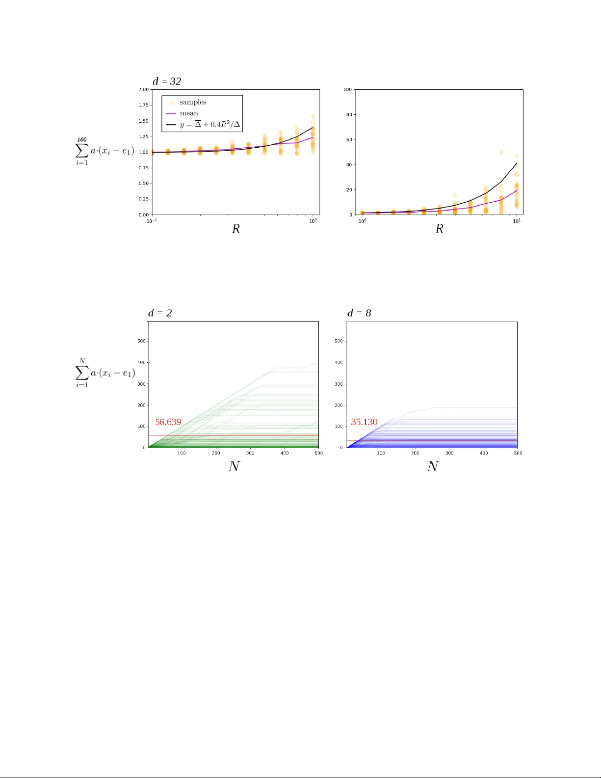
Optimalit y of the Subgradien t Algorithm in the Sto c hastic Setting Daron Anderson andersd3@tcd.ie Dep artment of Computer Scienc e and Statistics T rinity Col le ge Dublin Ir eland Douglas Leith doug.leith@scss.tcd.ie Dep artment of Computer Scienc e and Statistics T rinity Col le ge Dublin Ir eland Octob er 2019 abstract W e sho w that the Subgradient algorithm is universal for online learning on the simplex in the sense that it simultaneously ac hieves O ( √ N ) regret for adv ersarial costs and O (1) pseudo-regret for i.i.d costs. T o the b est of our knowledge this is the first demonstration of a universal algorithm on the simplex that is not a v arian t of Hedge. Since Subgradient is a p opular and widely used algorithm our results hav e immediate broad application. 1. Introduction In this pap er w e sho w that the Subgradient algorithm is univ ersal for online learning on the simplex in the sense that it ac hieves O ( √ N ) regret for adv ersarial sequences and O (1) pseudo-regret for i.i.d sequences. This complemen ts a recen t result b y [Mourtada and Ga ¨ ıffas(2019)] sho wing that the Hedge (Exp onen tial W eights) algorithm is also universal in the same sense. These tw o results are: (i) significant and interesting b ecause the Subgradient and Hedge algorithms are popular and widely used so improv ed results hav e immediate broad application, and (ii) surprising b ecause earlier lines of researc h on univ ersal algorithms required the dev elopmen t of complicated algorithms purp ose-built to be universal, whereas Subgradient and Hedge [Kivinen and W armuth(1997)] are simple and predate this line of researc h. Our subgradien t analysis is additionally in teresting b ecause: (i) it requires the dev elopmen t of a new metho d of pro of that may b e of wider application, and (ii) highlights fundamental differences b etw een the lazy and greedy v arian ts of Subgradient when it comes to univ ersality , namely lazy v arian ts are univ ersal whereas greedy v arian ts are not. The setup we consider is standard. Let b 1 , b 2 , . . . ∈ R d b e a sequence of cost v ectors. On turn n we know b 1 , . . . , b n − 1 (i.e. this is the full information rather than the bandit setting) and must select an action x n in the compact con vex domain X ⊂ R d with a mind to minimising the sum P N i =1 b i · x i . The r e gr et with resp ect to action x ∗ ∈ X is P N i =1 b i · ( x i − x ∗ ). It is well kno wn that when b 1 , b 2 , . . . are c hosen b y an adversary the Subgradient and Hedge algorithms (as w ell as others) hav e order O ( √ N ) regret for all x ∗ ∈ X simultaneously . When the sequence of cost v ectors is i.i.d we denote them b y a 1 , a 2 , . . . to av oid confusion. In the i.i.d case it is common to only consider X = S , where S is the simplex, and to b ound the pseudo-r e gr et E h P N i =1 a · ( x i − x ∗ ) i for 1 2 a = E [ a n ] and all x ∗ ∈ S . Algorithms are known (see b elo w for further discussion) that give O (1) pseudo-regret for b ounded i.i.d cost vectors. In this pap er we show that the lazy , anytime v ariant of the Subgradient algorithm has pseudo- regret at most O ( L 2 2 / ∆) for i.i.d cost vectors satisfying k a n k 2 ≤ L 2 , where ∆ = min { ∆ j : ∆ j > 0 } is the sub optimalit y gap and ∆ j = a · ( e j ∗ − e j ) for j ∗ ∈ arg min { a · e j : j = 1 , 2 , . . . , d } and e i the v ector with i ’th component 1 and all others 0. Subgradien t is already kno wn to ha ve O ( L 2 √ N ) adversarial regret. That is, the same Subgradien t algorithm sim ultaneously achiev es go od p erformance for adv ersarial loss sequences and for i.i.d sequences. 1.1. Related W ork. In recent years there has b een muc h in terest in universal algorithms, mainly in the bandit setting. F or example [Zimmert and Seldin(2018)] giv e a randomised algorithm that sim ultaneously achiev es O ( √ dN ) pseudo-regret in the antagonistic case and O (log ( N ) / ∆) pseudo- regret in the i.i.d case. These b ounds are the same order as the familiar Exp3.P and UCB algorithms [Bub ec k and Cesa-Bianchi(2012)] respectively . See [Seldin and Slivkins(2014), Zimmert and Seldin(2018), Auer and Chiang(2016), Seldin and Lugosi(2017), W ei and Luo(2018)] and references therein for more details. All of these universal algorithms resem ble Hedge in using potentials that are infin- itely ste ep at the b oundary of the simplex. Another line of work lo oks at combining algorithms for the tw o settings to obtain a univ er- sal meta-algorithm. One strategy is to start off with an algorithm suited to sto c hastic costs and then switch irreversibly to an adversarial algorithm if evidence accumulates that the data is non-sto c hastic. The other main strategy is to use reversible switc hes with the decision as to which algorithm (or com bination of algorithms) is used b eing up dated in an online manner. One such strategy is ( A, B )-Pro d prop osed by [Sani et al.(2014)Sani, Neu, and Lazaric]. F or com- bining tw o algorithms A and B with regret R A and R B the meta-algorithm has regret at most min  R B + 2 log 2 , R A + O ( √ N log N )  . Cho osing algorithm A to hav e O ( √ N log N ) adversarial regret (or b etter) and algorithm B to ha ve O (1) regret when the costs are i.i.d therefore means that the com bined algorithm has O ( √ N log N ) regret when costs are adv ersarial and O (1) regret when costs are i.i.d. Of course O ( √ N log N ) is muc h worse than the O ( √ N ) adversarial regret of algorithms suc h as Hedge and Subgradien t. W e also note that ( A, B )-Pro d uses the Prod algorithm whic h is equiv alen t to Hedge with a second-order correction. A related line of work uses the fact that algorithms suc h as Hedge can achiev e go od regret if the step size is tuned to the setting of in terest. The approach tak en is therefore to try to select the step size in an online fashion, see for example [Erven et al.(2011)Erven, Ko olen, Ro oij, and Grun wald]. With regard to the impact of step size on performance, [Huang et al.(2016)Huang, Lattimore, Gy¨ orgy , and Szep esv´ a ri] consider the performance of the FTL algorithm with i.i.d costs, the FTL algorithm b eing equiv a- len t to lazy Subgradien t with step-size 1. They show that for i.i.d costs for which the mean a has a unique minimiser and k a n k ∞ ≤ L ∞ the pseudo-regret of FTL on the simplex (in fact, for any p olyhedron) is O ( L 3 ∞ d/r 2 ), where r is essentially the size of the ball around mean cost a within whic h the minimizer is unique. This is one of the few results on Subgradien t p erformance for i.i.d losses. Note, how ev er that FTL has O ( N ) regret for adversarial costs and must b e incorp orated in to a meta-algorithm to accoun t for that case. In the foregoing w ork the search for univ ersality has en tailed the dev elopment of new algorithms, almost all of whic h are v ariations on Hedge. Recently , a striking result b y [Mourtada and Ga ¨ ıffas(2019)] 3 estabished that in the full information setting this is unnecessary . The standard Hedge algo- rithm, without mo dification, simultaneously achiev es O ( L ∞ √ N ) regret in the adversarial case and O ( L 2 ∞ log( d ) / ∆) pseudo-regret in the i.i.d case for b ounded costs k a n k ∞ ≤ L ∞ . This is app ealling b oth b ecause of the simplicity and p opularit y of the Hedge algorithm and b ecause of the tight na- ture of the bounds i.e. there is no need to pay for O (1) i.i.d pseudo-regret b y suffering O ( √ N log N ) adv ersarial regret. It also raises the question as to whether the other main class of widely used algorithms, namely Subgradient, is in fact also universal. 1.2. Results and Con tribution. Our Theorem 2 sa ys that lazy , an ytime Subgradient has pseudo- regret O ( L 2 2 / ∆) in the i.i.d case, where L 2 b ounds the 2-norm of the cost v ectors. It follo ws that this v ariant of Subgradient simultaneously ac hieves O ( L 2 √ N ) regret in the adversarial case and O ( L 2 2 / ∆) pseudo-regret in the i.i.d case for b ounded costs k a n k 2 ≤ L 2 . T o the b est of our kno wledge this is the first demonstration of a univ ersal algorithm on the simplex that is not a v ariant of Hedge. Since Subgradient is a p opular and widely used algorithm our results ha ve immediate broad application. The metho d of pro of of Theorem 2 app ears to b e new. Rather than follow a sequence of actions inside the simplex, w e follo w the sequence of unpro jected actions, and sho w the sequence ev entually passes with high probability into the normal cone of the optimal vertex. Hence the pro jected action ev en tually snaps to the correct vertex. This b eha viour, whereb y Subgradien t conv erges to the optimal action in finite-time, is qualitatively differen t from Hedge-type algorithms where the actions only approach the optimal vertex asymptotically . This new metho d of pro of is likely to b e of wider application. A tec hnical tool used that seems new in the con text of Online Optimisation is the v ector concen tration inequalit y Theorem 3.5 of [Pinelis(1994)]. F or comparison it is possible to get O  P d j =1 L 2 2 / ∆ j  pseudo-regret bounds for Subgradient using only scalar concen tration inequalities for eac h comp onen t, and to obtain a O  log( d ) L 2 2 / ∆  b ound by using the adv ersarial b ound ov er an initial segment of turns and then a probabilistic b ound ov er the remainder. How ev er the Pinelis v ector inequalit y allows us to tigh ten these b ounds to to the dimension-free O ( L 2 2 / ∆). Remo ving the log( d ) factor is a significant impro vemen t when d is large. Theorem 4 extends our analysis to include tail b ounds on the pseudo-regret. Namely , for Sub- gradien t there is c > 0 and C > 0 indep endent of η , ∆ with P N X i =1 a · ( x i − x ∗ ) > c + L 2 2 ∆ δ ! ≤ O  e − C δ  for all δ sufficiently large. One adv an tage of Subgradien t is it can b e applied with actions on arbitrary domains X , not just the simplex S . In Section 4.1, how ev er, we show this can break the results of Theorem 2. Namely , for each ε > 0 there is a domain and i.i.d cost vectors that giv e pseudo-regret Ω( N 1 / 2 − ε ). Thus the i.i.d pseudo-regret can b e almost as bad as the O ( √ N ) worst-case regret. These domains hav e the form { ( x, y ) ∈ R 2 : y ≥ x α } for α > 2 and are not strictly conv ex at the origin. In Section 4.2 we show the use of lazy rather than greedy Subgradient is imp ortan t in ac hieving universal p erformance. W e giv e an example that sho ws greedy Subgradient is to o sensitive to adapt to the i.i.d setting. 4 2. Terminology and Not a tion Throughout d is the dimension of the online optimisation problem. W e write x ( j ) for the compo- nen ts of x ∈ R d and e 1 , e 2 , . . . , e d ∈ R d for the co ordinate vectors and 1 for the vector (1 , . . . , 1) ∈ R d . Define the d -simplex S = { x ∈ R d : all x ( j ) ≥ 0 and 1 · x = 1 } . F or an y function f : X → R we write argmin { f ( x ) : x ∈ X } for the set of minimisers. Each linear function on the simplex is minimised on some v ertex. Hence min { a · x : x ∈ S } = min { a · e j : j ≤ d } . W e write k ·k for the Euclidean norm and for any con vex X ⊂ R d w e write P X ( x ) = argmin {k y − x k 2 : y ∈ X } for the Euclidean pro jection of x on to X . Thoughout the c ost ve ctors a 1 , a 2 , . . . ∈ R d are realisations of a sequence of i.i.d random v ariables with each E [ a i ] = a . When we write b 1 , b 2 , . . . we mak e no assumptions on whether the cost vectors are i.i.d or otherwise. W e assume b ounds of the form k a i − a k ≤ R and k a i k ≤ L . F or cost vectors b 1 , b 2 , . . . the r e gr et of an action sequence x 1 , . . . , x N is defined as P N i =1 b i · ( x i − x ∗ ) for x ∗ ∈ argmin P N i =1 b i · x . F or sto c hastic cost vectors a 1 , a 2 , . . . the pseudo-r e gr et of the action sequence is E h P N i =1 a · ( x i − x ∗ ) i for x ∗ ∈ argmin a · x . Here the exp ectation is taken ov er the domain of a 1 , . . . , a N . By p erm uting the co ordinates if neccesary we assume e 1 is a minimiser of a and that the differ- ences ∆ j = a · ( e j − e 1 ) satisfy 0 = ∆ 1 ≤ ∆ 2 ≤ . . . ≤ ∆ d . The p erm utation is part of the analysis only , and our algorithm do es not require access to it. W e write ∆ = ∆ 2 = min { ∆ j : ∆ j > 0 } . 3. Pseudo-Regret The subgradient algorithm is one of the simplest and most familiar algorithms for online conv ex optimisation. The anytime version Algorithm 1 do es not need the time horizon in adv ance. In this algorithm the step size on turn n is η / √ n − 1 where η > 0 is a design parameter. Algorithm 1: Anytime Subgradient Algorithm Data: Compact conv ex subset X ⊂ R d . Parameter η > 0. 1 select action x 1 = P X (0) 2 pa y cost a 1 · x 1 3 for n = 2 , 3 , . . . do 4 reciev e a n − 1 5 y n = − η  a 1 + . . . + a n − 1 √ n − 1  6 select action x n = P X ( y n ) 7 pa y cost a n · x n The subgradien t algorithm is known to hav e O ( L √ N ) regret. See [Shalev-Shw artz(2012)] and [Zink evich(2003)]. Theorem 1. F or cost vectors b 1 .b 2 , . . . , b N with all k b i k ≤ L Algorithm 1 with parameter η > 0 has regret satisfying N X i =1 b i · ( x i − x ∗ ) ≤ LD +  1 2 η kX k 2 + 2 η L 2 2  √ N 5 for kX k = max {k x k : x ∈ X } and D the diameter of X . In particular for X = S and η = 1 / 2 L we ha ve N X i =1 b i · ( x i − x ∗ ) ≤ √ 2 L + 2 L √ N . Pr o of. See App endix A.  Our main result is that, in addition to the ab ov e b ound, the algorithm adapts to the sto c hastic case to ha ve O ( L 2 2 / ∆) pseudo-regret. In particular the b ound is indep enden t of the dime nsion of the problem. Theorem 2. Supp ose the cost v ectors a 1 , a 2 , . . . are indep enden t with all k a i k ≤ L 2 and k a i − a k ≤ R 2 . Then Algorithm 1 run on the simplex has pseudo-regret at most E " ∞ X i =1 a · ( x i − x ∗ ) ≤ # √ 2 L + (1 + 2 η 2 L 2 2 ) L 6 + 3 /η 2 + 6 L 2 2 + 72 R 2 2 e − 1 / 2 η 2 R 2 ∆ . (1) for ∆ = min { ∆ j : ∆ j > 0 } . In particular for η = 1 / 2 L the pseudo-regret is at most E " ∞ X i =1 a · ( x i − x ∗ ) # ≤ 2 L + 18 L 2 2 + 72 R 2 2 ∆ The strategy is to use Theorem 1 ov er an initial segment of the turns and a probabilistic b ound o ver the final segment. Over that segmen t we are interested in conditions that make − η √ n P n i =1 a i pro ject on to the con vex hull of { e 1 , . . . , e k } as this ensures the regret is at most ∆ k . T o that end w e use the following lemma that is pro ved in the App endix. Lemma 1. Supp ose w ∈ R d has t wo co ordinates k , ` with w k − w ` ≥ 1. Then P S ( w ) has ` - co ordinate zero. No w we sho w ho w smaller errors make us select b etter vertices. Lemma 2. Suppose n ≥ 9 / ∆ 2 j η 2 . Then for   1 n P n i =1 ( a − a i )   ∞ ≤ ∆ j / 3 the action x n +1 is in the con vex hull of e 1 , . . . , e j − 1 and the pseudo-regret for that round is at most ∆ j − 1 . Pr o of. Since x n +1 = P S  − η √ n P n i =1 a i  the previous lemma says it is enough to sho w for ` ≥ j that η √ n P n i =1 a i ( ` ) − η √ n P n i =1 a i (1) ≥ 1. T o that end write η √ n n X i =1  a i ( ` ) − a i (1)  = η √ n n X i =1 ∆ ` + η √ n n X i =1  a i ( ` ) − a (1)  + η √ n n X i =1  a (1) − a i (1)  ≥ η ∆ ` √ n − 2 η √ n    n X i =1 ( a − a i )    ∞ ≥ η ∆ j √ n − 2 η ∆ j 3 √ n = η ∆ j 3 √ n The assumption on n makes the righ t-hand-side at least 1.  No w we pro ve our b ound o ver the final segment. Lemma 3. Supp ose a 1 , a 2 , . . . hav e k a i − a k ∞ ≤ R 2 . Then for n 0 > d 9 / ∆ 2 η 2 e Algorithm 1 giv es E " ∞ X i = n 0 a · ( x i − e 1 ) # ≤ 72 R 2 2 ∆ exp  − 1 2 η 2 R 2 2  . 6 Pr o of. W rite the distinct elements of { ∆ 2 , ∆ 3 , . . . , ∆ d } in increasing order as ∆(2) < . . . < ∆( K ) for some K ≤ d . Define eac h Γ( j ) = ∆( j ) 2 / 18 R 2 2 . Theorem says each P  1 n   P n i =1 ( a i − a )   ≥ ∆( j ) / 3  ≤ 2 exp − Γ( j ) n . Since k x k ∞ ≤ k x k we can combine Lemmas 1 and 2 for n ≥ n 0 to b ound the complementary CDF: P  a · ( x n +1 − e 1 ) > x  ≤        2 e − Γ(2) n 0 < x ≤ ∆(2) 2 e − Γ( k ) n ∆( k − 1) < x ≤ ∆( k ) with k ≥ 3 0 ∆( K ) < x Lemma 9 lets us integrate the piecewise function to get E [ a · ( x n +1 − e 1 )] ≤ 2∆(2) e − Γ(2) n + 2 P d k =3 (∆( k ) − ∆( k − 1)) e − Γ( k ) n . Now sum o ver n and observe, since the summands are decreasing, the sums are b ouded b y the integrals: E " ∞ X i = n 0 a · ( x i − e 1 ) # ≤ 2∆(2) ∞ X i = n 0 e − Γ(2) n + 2 d X k =3 ∞ X i = n 0 (∆( k ) − ∆( k − 1)) e − Γ( k ) n (2) ≤ 2∆(2) Z ∞ i = n 0 e − Γ(2) n + 2 d X k =3 Z ∞ i = n 0 (∆( k ) − ∆( k − 1)) e − Γ( k ) n ≤ 2∆ 2 Γ(2) + 2 d X k =3 ∆( k ) − ∆( k − 1) Γ( k ) ! e − Γ(2) n 0 = 36 R 2 2 1 ∆ 2 + d X k =3 ∆ k − ∆( k − 1) ∆( k ) 2 ! e − Γ(2) n 0 T o b ound the ab o ve use the integral inequality R b a f ( x ) dx ≥ ( a − b ) min { f ( x ) : a ≤ x ≤ b } . F or f = 1 /x 2 w e get ∆ k − ∆ k − 1 ∆ 2 k ≤ R ∆ k ∆ k − 1 dx x 2 . Hence the ab o ve sum is at most d X k =3 ∆ k − ∆ k − 1 ∆ 2 k ≤ d X k =3 Z ∆ k ∆ k − 1 dx x 2 = Z ∆ d ∆ 2 dx x 2 ≤ Z ∞ ∆ 2 dx x 2 = 1 ∆ 2 . and we get E  P ∞ i = n 0 a · ( x i − e 1 )  ≤ 72 R 2 2 ∆ 2 e − Γ(2) n 0 . Recall the definitions of n 0 and Γ(2) to see the exp onen t is at least ∆ 2 18 R 2 2 9 ∆ 2 η 2 = 1 2 η 2 R 2 2 .  Pr o of of The or em 2. F or X the simplex k X k 2 = 2 and D = √ 2. Hence for n 0 = d 9 / ∆ 2 η 2 e Theorem 2 gives the regret b ound n 0 X i =1 a i · ( x i − x ∗ ) ≤ √ 2 L +  1 η + 2 η L 2 2  √ n 0 ≤ √ 2 L +  1 η + 2 η L 2 2  p 1 + 9 / ∆ 2 η 2 By concavit y the square ro ot is at most p 1 + 9 / ∆ 2 η 2 ≤ p 9 / ∆ 2 η 2 + 1 2 r η 2 ∆ 2 9 = 3 η ∆ + η ∆ 6 ≤ 3 η ∆ + η L 6 7 and we get n 0 X i =1 a i · ( x i − x ∗ ) ≤ √ 2 L + (1 + 2 η 2 L 2 2 ) L 6 +  1 η 2 + 2 L 2  3 ∆ . Hence the same b ound holds for the exp ected regret. Since the pseudo-regret is alwa ys less than exp ected regret we can com bine the ab o ve with the previous lemma to complete the pro of.  As men tioned in Section 2 our b ound has differen t b eha viour to that of [Mourtada and Ga ¨ ıffas(2019)] for Hedge, and is more appropriate if the cost vectors come from a sphere rather than a cub e. On the other hand our b ound is dimension-indep enden t. 3.1. Better Constants. Theorem 2 can b e improv ed by replacing the constants R 2 , L 2 with the smaller constan ts that arise when w e ignore the comp onen ts of the cost v ectors that are p erpen- dicular to the simplex. Definition 1. Let P : R d → V b e the pro jection onto the conv ex hull V = { x ∈ R d : P d j =1 x ( j ) = 0 } of the simplex. Define e L 2 = sup {k P a n k : n ∈ N } and e R 2 = sup {k P ( a n − a ) k : n ∈ N } . T o write down e L 2 and e R 2 explicitly recall the Euclidean norm can b e computed with resp ect to an y orthonormal basis. Hence we can choose an orthonormal basis u 1 , . . . , u d − 1 for V and then add u d = 1 √ d 1 to get an orthonormal basis for the whole space. The pro jection of each x = P d j =1 c j u j on to V is just P d − 1 j =1 c j u j and the norm of the pro jection is k P x k = q P d − 1 j =1 c 2 j = q P d j =1 c 2 j − c 2 d = q P d j =1 c 2 j − ( u d · x ) 2 = q k x k 2 − 1 d ( 1 · x ) 2 . Hence we can write e L 2 2 = sup  k a n k 2 − 1 d  P d j =1 a n ( j )  2 : n ∈ N  (3) e R 2 2 = sup  k a n − a k 2 − 1 d  P d j =1 a n ( j ) − a ( j )  2 : n ∈ N  Theorem 3. Theorems 1 and 2 hold with the constants L and R replaced with e L 2 and e R 2 . Pr o of. W e claim the actions giv en any cost v ectors b 1 , b 2 , . . . are the same as those giv en the pro jections P b 1 , P b 2 , . . . . F rom line 5 of Algorithm 1 we see it is enough to show for eac h x ∈ R d that P S ( x ) = P S ( P V ( x )). T o that end consider the sphere S with centre x and radius k x − P S ( x ) k . This sphere meets the simplex at the single p oin t P S ( x ). The intersection S ∩ V is a circle centred at P V ( x ) that meets the simplex at the p oin t P S ( x ). It follows P S ( x ) is the pro jection of P V ( x ) on to the simplex as required. It follows a 1 , a 2 , . . . give the same actions as P a 1 , P a 2 , . . . . Hence the b ounds in Theorems 1 and 2 hold with e L 2 , e R 2 in place of L, R and E [ P ∞ i =1 P a · ( x i − x ∗ )] on the left for eac h x ∗ ∈ S . T o complete the proof w e claim P a · ( x i − x ∗ ) = a · ( x i − x ∗ ). This is equiv alent to ( P a − a ) · ( x i − x ∗ ) = 0 whic h holds b ecause P a − a is p erp endicular to V and x i − x ∗ is contained in V .  4. Counterexamples One shortcoming of Hedge-type algorithms is they only make sense when the action set is the simplex. This is b ecause they use p oten tials that are infinitely ste ep on the b oundary . On the 8 other hand the quadratic p oten tial from Subgradien t is defined everywhere and the algorithm can b e applied to arbitrary action sets. This raises the question of what kinds of domains w e can use to replace the simplex while keeping the order b ounds from Theorems 2 and 3. 4.1. Bey ond the Simplex. Here we giv e an example of a curved domain where the order b ounds in Theorems 2 and 3 fail. Example 1. Supp ose we run Algorithm 1 with parameter η = 1 and domain Y = { ( x, y ) ∈ R 2 : y ≥ | x | 3 and x ≤ 1 } . There is a sequence a 1 , a 2 , . . . of i.i.d cost vectors such that E " n X i =1 a · ( x i − x ∗ ) # ≥ Ω( 4 √ n ) . Pr o of. Let the cost vectors b e a n = ( B n , 1) for B 1 , B 2 , . . . indep enden t with eac h P ( B i = 1) = P ( B i = − 1) = 1 / 2. The central limit theorem says η √ n P n i =1 B i tends to a normal distribution. Hence there are m ∈ N and c > 0 suc h that for all n ≥ m w e ha ve P  η √ n P n i =1 B i > 1  ≥ c . W e claim that if η √ n P n i =1 B i > 1 o ccurs then a · ( x n +1 − x ∗ ) ≥ 6 − 3 / 2 n − 3 / 4 . Hence we ha ve E " n X i>M a · ( x i − x ∗ ) # ≥ c n X i>m 6 − 3 / 2 i − 3 / 4 ≥ c 6 − 3 / 2 Z n m +1 x − 3 / 4 dx ≥ c 6 − 3 / 2 4  4 √ n − 4 √ m + 1  . It follows the pseudo-regret is at least − 2 k a k m + c 6 − 3 / 2 4  4 √ n − 4 √ m + 1  ≥ Ω  4 √ n  . T o prov e the claim supp ose η √ n P n i =1 B i > 1 and write x n +1 = ( x, | x | 3 ). Since a = (1 , 0) has minimiser x ∗ = (0 , 0) w e ha ve a · ( x n +1 − x ∗ ) = x 3 . Since x n +1 is the pro jection of y n +1 = − 1 √ n P n i =1 a i on to X we hav e either (a) x n +1 = ( ± 1 , 1) or (b) x n +1 is the pro jection of y n +1 on to the graph y = | x | 3 . In the first case a · ( x n +1 − x ∗ ) = 1. In the second case y n +1 is in the left quadrant and so x < 1. Since x n +1 is the pro jection of y n +1 w e know y n +1 − x n +1 is outw ard normal to the graph. Expand the definition to see y n +1 − x n +1 = − 1 √ n n X i =1 a i − x n +1 = − 1 √ n n X i =1 B i − x, − √ n − x 3 ! Since x < 1 the slop e at x n +1 is − 3 x 2 . Hence the out wards normal p oints along ( − 3 x 2 , − 1). Rescale to see 1 √ n n X i =1 B i + x = 3 x 2 ( √ n + x 3 ) = ⇒ 1 < 3 x 2 ( √ n + x 3 ) < 6 x 2 √ n where we hav e used | x | ≤ 1. The ab o ve implies x ≥ 6 − 1 / 2 n − 1 / 4 and so a · ( x n +1 − x ∗ ) = | x | 3 ≥ 6 − 3 / 2 n − 3 / 4 . This completes the pro of.  More generally we can take the domain Y α = { ( x, y ) ∈ R 2 : y ≥ | x | α and x ≤ 1 } for any α > 2. Then an analogous pro of to the ab o ve shows the pseudo-regret has order Ω( N 1 − α 2( α − 1) ). Hence we get the following 9 Lemma 4. Let ε > 0 b e arbitrary . There exists a compact con vex domain Y ⊂ R 2 and i.i.d sequence a 1 , a 2 , . . . of cost vectors with E [ a i ] = a such that running Algorithm 1 with an y parameter η = 1 giv es n X i =1 a · ( x i − x ∗ ) ≥ Ω( n 1 / 2 − ε ) . On the other hand [Huang et al.(2016)Huang, Lattimore, Gy¨ orgy , and Szep esv´ ari] show w e can get O (log N ) regret against i.i.d cost v ectors on each Y α pro vided the minimiser is not the origin. Their Theorem 3.3 says that since f ( x ) = | x | α has nonzero second deriv ativ e aw a y from the origin w e can get O (log n ) regret by running F ollow-the-Leader. Lik ewise since f ( x ) = x 2 has nonzero deriv ative ev erywhere the same theorem gives a O (log n ) b ound on Y 2 for any minimiser. Lemma 4 sa ys that as α → ∞ the worst-case b eha viour of Subgradient approaches Ω( √ n ). It is in teresting that for α = ∞ the domain is the b o x [ − 1 , 1] × [0 , 1], and a similar argumen t to Theorem 1 says Subgradient gives O (1) regret o ver the b o x. 4.2. Greedy Subgradient is not Univ ersal. The fact that Theorems 2 and 3 are pro ved for the Lazy Subgradient algorithm rather than Greedy Subgradien t is imp ortan t. Indeed the theorems fail if we instead use the greedy v ersion. The reason is that Greedy is to o sensitive to next cost v ector to remain on the optimal vertex. Recall the greedy Subgradien t on domain X chooses actions x 2 , x 3 . . . recursively by y n +1 = x n − η √ n a n and x n +1 = P X ( y n +1 ). It is straigh tforward to come up with i.i.d examples where the pseudo-regret is Ω( √ N ). This matches the worst-case b ound for regret [Zinkevic h(2003)]. Example 2. Supp ose we run the greedy Subgradient algorithm on the 2-simplex with parameter η = 1. There is a sequence a 1 , a 2 , . . . of i.i.d cost vectors with E [ a i ] = a and E " n X i =1 a · ( x i − x ∗ ) # ≥ Ω( √ n ) . Pr o of. Let V = { x ∈ R d : P d j =1 x ( j ) = 0 } b e the affine span of the simplex. In Theorem 3 we sho w that for any x ∈ R d that P S ( x ) = P S ( P V ( x )). Hence running Greedy subgradient on the 2-simplex with cost vectors a n = ( a n (1) , a n (2)) is equiv alen t to running it on domain [ − 1 , 1] with cost vectors (scalars) a n (1) − a n (2) 2 . F or ease of notation we will work in the second setting. Let the cost vectors (scalars) b e a n = 1 with probability 3 / 4 and a n = − 1 with probability 1 / 4. Then a = 1 / 2 and the minimiser is x ∗ = − 1. W e claim each x n +1 ≥ − 1 + 1 √ n with probabilit y at least 1 / 4. Hence E [ a · ( x n +1 − x ∗ )] ≥ 1 4 √ n and so E " n X i =2 a · ( x i − x ∗ ) # ≥ n − 1 X i =1 1 4 √ n ≥ Z n − 1 1 dx 4 √ x = √ n − 1 − 1 2 ≥ Ω( √ n ) . By definition x n +1 = P X ( x n − a n √ n ). Since x n ∈ [ − 1 , 1] we hav e x n ≥ − 1. With probability 1 / 4 w e hav e a n = − 1 and so x n − a n √ n = x n + 1 / √ n ≥ − 1 + 1 / √ n as required.  10 5. T ail Bounds In this section w e sho w the v alue P ∞ i =1 a · ( x i − e 1 ) is unlikely to stra y to o far from the exp ectation. Recall Theorem 1 says E  P ∞ i =1 a · ( x i − e 1 )  ≤ O ( L 2 2 / ∆). Next we show the the probability of the co efficien t b eing large shrinks exp onen tially . Theorem 4. Supp ose the cost v ectors a 1 , a 2 , . . . are indep enden t with all k a i k ≤ L 2 and k a i − a k ≤ R 2 . Then Algorithm 1 run on the simplex has tail b ound P ∞ X i =1 a · ( x i − e 1 ) > 2 L 2 + L 2 2 ∆ t ! ≤ (1 + 36 R 2 ) exp  − t 24 R 2  for all t ≥ 3 L 2 2  2 L 2 + √ 2 η + √ 2 3 ∆  2 . Lik e b efore we derive separate b ounds o ver initial and final segments. F or the final segment w e ha ve the lemma. Lemma 5. F or eac h n > 9 / ∆ 2 η 2 w e hav e P ∞ X i>n a · ( x i − e 1 ) = 0 ! ≥ 1 − 36 R 2 2 exp  − ∆ 2 18 R 2 n  Pr o of. Combine Lemma 2 and Theorem 5 to see P ( x i +1 6 = e 1 ) ≤ 2 exp  − ∆ 2 18 R 2 i  . T ake a union b ound to see P ( x i +1 6 = e 1 for some i ≥ n ) is at most ∞ X i = n 2 exp  − ∆ 2 18 R 2 i  ≤ Z ∞ n 2 exp  − ∆ 2 18 R 2 x  dx = 36 R 2 ∆ 2 exp  − ∆ 2 18 R 2 n  . T o finish the pro of observe if x n +1 = x n +2 = . . . = e 1 the pseudo-regret after turn n is zero.  No w we b ound the initial segment. Lemma 6. F or eac h n ∈ N and t > 0 w e ha ve P n X i =1 a · ( x i − e 1 ) > 2 L 2 + (2 L 2 + t ) √ n ! ≤ exp  − t 2 4 R 2  Pr o of. By Theorem 1 we hav e n X i =1 a · ( x i − e 1 ) = n X i =1 a i · ( x i − e 1 ) + n X i =1 ( a − a i ) · ( x i − e 1 ) ≤ √ 2 L 2 + 2 L 2 √ n + n X i =1 ( a − a i ) · ( x i − e 1 ) F or the final sum Lemma 10 says X i = ( a − a i ) · ( x i − e 1 ) is a martingale difference sequence with resp ect to a 1 , a 2 , . . . . Since each | X i | ≤ k a − a i kk x i − e 1 k ≤ √ 2 R Lemma 7 says the sum exceeds t √ n with probability at most exp  − t 2 4 R 2  .  11 No w we com bine the previous tw o lemmas. Pr o of of The or em 4. F or eac h t ≥ max n √ 2 η , √ 2 3 ∆ o w e ha ve 9 t 2 2∆ 2 ≥ 9 ∆ 2 η 2 and we can com bine the previous tw o lemmas with n = l 9 t 2 2∆ 2 m . F or the left-hand-side of Lemma 6 we hav e (2 L 2 + t ) √ n ≤ (2 L 2 + t ) r 9 t 2 2∆ 2 + 1 ≤ (2 L 2 + t ) r 9 t 2 ∆ 2 = 3 ∆ (2 L 2 + t ) t where the second inequalit y uses t ≥ √ 2 3 ∆ to see 1 ≤ 9 t 2 2∆ 2 . Hence we ha ve (2 L 2 + t ) √ n ≤ 3 ∆ (2 L 2 + t ) t = 3 ∆  ( t + L 2 ) 2 − L 2 2  ≤ 3 ∆ ( t + L 2 ) 2 F or the right-hand-side of Lemma 5 we ha ve exp  − ∆ 2 18 R 2 n  = exp  − ∆ 2 18 R 2  9 t 2 2∆ 2  ≤ exp  − t 2 4 R 2  Hence the tw o lemmas combine to give P ∞ X i =1 a · ( x i − e 1 ) > 2 L 2 + 3 ∆ ( t + L 2 ) 2 ! ≤ (1 + 36 R 2 ) exp  − t 2 4 R 2  . Define δ = t + L 2 to see for all δ ≥ L 2 + max n √ 2 η , √ 2 3 ∆ o that P ∞ X i =1 a · ( x i − e 1 ) > 2 L 2 + 3 ∆ δ 2 ! ≤ (1 + 36 R 2 ) exp  − ( δ − L 2 ) 2 4 R 2  If in addition δ ≥ 2 L 2 w e hav e ( δ − L 2 ) 2 ≥ ( δ / 2) 2 . Hence for all δ ≥ 2 L 2 + max n √ 2 η , √ 2 3 ∆ o w e ha ve P ∞ X i =1 a · ( x i − e 1 ) > 2 L 2 + 3 ∆ δ 2 ! ≤ (1 + 36 R 2 ) exp  − δ 2 8 R 2  Finally define t = 3 δ 2 /L 2 2 and the ab ov e b ecomes P ∞ X i =1 a · ( x i − e 1 ) > 2 L 2 + L 2 2 ∆ t ! ≤ (1 + 36 R 2 ) exp  − t 24 R 2  for all t ≥ 3 L 2 2  2 L 2 + √ 2 η + √ 2 3 ∆  2  By the same argumen t as Theorem 3 we can replace the constan ts in Theorem 4 with the smaller constan ts (3). 12 6. Simula tions Here we plot the results of some sim ulations. W e compare the co efficien ts in Theorem 2 to those observ ed empirically . Our sim ulations suggest the true constants are t w o orders of magnitude smaller than our theoretical b ounds. F or each simulation w e fix ∆ = η = 1. The i.i.d sequence a 1 , a 2 , . . . , ∈ R d w as generated as a n = a + RN n for N 1 , N 2 , . . . drawn uniformly from the ( d − 1)-dimensional unit sphere. Sampling on the unit sphere w as done b y drawing inp enden t standard normals U 1 , . . . , U d and normalising the vector ( U 1 , . . . , U d ). See [Muller(1959)] Section 4 for a pro of of this metho d. Figure 1. Scatter plots of noise R against pseudo-regret for a = (0 , 1 . . . , 1) and d = 2. F or eac h R -v alue we to ok 25 samples. Eac h sample ran for 500 turns. The horizon tal axes use a log scale. Some larger samples are excluded from the plot. T o chose a goo d comparator consider the expression 3 /η 2 + 72 R 2 2 e − 1 / 2 η 2 R 2 on the righ t-hand-side of Theorem 2. By setting x = 1 /η 2 and differentiating we find the minimiser 1 /η 2 = 2 R 2 2 log 12 giv es minim um 6(1 + log 12) R 2 2 ' 21 R 2 . On the other hand for R ≥ 1 and the η = 1 used in the sim ulations we hav e 72 R 2 2 e − 1 / 2 η 2 R 2 ≥ (72 / √ e ) R 2 2 ≥ 43 R 2 . These b ounds seem to o c onserv ativ e as Figures 1 and 2 suggest ∆ + 0 . 4 R 2 / ∆ for ∆ = 1 d P d j =1 ∆ j is a more realistic b ound. Figures 3 and 4 also suggests higher dimensions r e gularise the data, lo wering the mean and significan tly low ering the v ariance. Another observ ation is that − even for large noise lev els − the b eha viour seems to stabilise faster than the analysis suggests. Similar to (2) we ha ve for n 0 sufficien tly high the b ound: E " ∞ X i = n 0 a · ( x i − e 1 ) # ≤ 2∆(2) N X i = n 0 e − Γ(2) n + 2 d X k =3 ∞ X i = n 0 (∆( k ) − ∆( k − 1)) e − Γ( k ) n for Γ( k ) = 18∆( k ) 2 R 2 . In Figures 3 and 4 we ha ve ∆( k ) = 1 and R 2 2 = 100 and the second sum v an- ishes. Replace the sum with an in tegral to see the righ t-hand-side is approximately 2 Γ(2) e − Γ( k ) n 0 = 3600 e − n 0 / 1800 . This suggests w e must wait until the order of turn n 0 = 1800 log 3600 ' 15000 b efore the b eha viour stabilises. How ev er Figures 3 and 4 suggest N = 500 turns is enough for low dimensions and N = 100 for higher dimensions. 13 Figure 2. Scatter plots of noise R against pseudo-regret for a = (0 , 1 . . . , 1) and d = 32. F or each R -v alue we to ok 25 samples. Each sample ran for 100 turns. The horizon tal axes use a log scale. Figure 3. Simultaneous line plots of 100 instances with a = (0 , 1 , . . . , 1) and R = 10. Eac h instance ran for 500 turns. The red line is the a verage of P 500 i =1 a · ( x i − e 1 ) o ver the 100 instances. The ab ov e simulations use a = (0 , 1 , . . . , 1) b ecause all other exp ectations w e tried gav e b etter p erformance. Tw o extreme cases are a = (0 , 1 , 2 , . . . , d − 1) and a = (0 , . . . , 0 , 1). The first gives mo derately b etter p erformance in the long-run: The large cost on turn 1 and differences b et w een arms mak es the pseudo-regret stabilise faster and giv es a steep er shoulder to the graph. The second giv es significantly b etter p erformance. A cknowledgements This work was supp orted by Science F oundation Ireland grant 16/IA/4610. 14 Figure 4. Simultaneous line plots of 100 instances with a = (0 , 1 , . . . , 1) and R = 10. Eac h instance ran for 100 turns. The red line is the a verage of P 100 i =1 a · ( x i − e 1 ) o ver the 100 instances. Figure 5. Sim ultaneous line plots of 100 instances with d = 8 and R = 10. Each instance ran for 500 turns. The red line is the a verage of P 500 i =1 a · ( x i − e 1 ) ov er the 100 instances. Appendix A: Regret in the General Setting Here we give the pro of the subgradient algorithm with suitable parameter has regret O  L √ N  . The pro of uses the techniques from [Shalev-Sh wartz(2012)] mo dified sligh tly to not men tion the time horizon. Theorem 1 F or cost vectors b 1 .b 2 , . . . , b N with all k b i k ≤ L Algorithm 1 with parameter η > 0 has regret satisfying N X i =1 b i · ( x i − x ∗ ) ≤ LD +  1 2 η kX k 2 + 2 η L 2 2  √ N 15 for kX k = max {k x k : x ∈ X } and D the diameter of X . In particular for X = S and η = 1 / 2 L w e ha ve N X i =1 b i · ( x i − x ∗ ) ≤ √ 2 L 2 + 2 L 2 √ N . Pr o of. F or n > 1 define the functions R n ( x ) = √ n − 1 2 η k x k 2 . First we show eac h x n is the unique minimiser of P n − 1 i =1 b i + R n ( x ). Since rescaling by a positive constant do es not change the minimisers the function has the same minimisers as k x k 2 + 2 η √ n − 1 n − 1 X i =1 b i · x =    x + η √ n − 1 n − 1 X i =1 b i    2 − η 2 n − 1  n − 1 X i =1 b i  2 (4) Since the last term is constant the ab o v e has global minim um at x = − η √ n − 1 P n − 1 i =1 b i . This is the p oint y n in the algorithm description. Lemma 7 says the minim um on X is the pro jection of the global minimum. Namely the p oint x n = P X ( y n ) as required. No w define the functions Q 2 ( x ) = R n ( x ) + b 1 · x + b 2 · x Q n ( x ) = R n ( x ) − R n − 1 ( x ) + b n · x for n > 2 . Clearly each P n i =2 Q i = P n i =1 b i · x + R n ( x ). Lemma 3.1 of [Cesa-Bianc hi and Lugosi(2006)] sa ys P N i =2 Q i ( z i ) ≤ P N i =2 Q i ( x ∗ ) where z n are an y minimisers of P n i =2 Q i o ver X and x ∗ ∈ X is arbitrary . Expanding b oth sides we get b 1 · z 2 + N X i =2 b i · z i + 1 2 η N X i =2 ( √ n − 1 − √ n − 2) k z i k 2 ≤ N X i =1 b i · x ∗ + √ N 2 η k x ∗ k 2 . Since the second sum is nonnegative we can neglect it. Bringing terms to the left and using k x ∗ k ≤ kX k we get b 1 · ( z 2 − x ∗ ) + N X i =2 b i · ( z i − x ∗ ) ≤ √ N 2 η kX k 2 . T o get regret on the left-hand-side add b 1 · ( x 1 − z 2 ) + P N i =2 b i · ( x i − z i ) to b oth sides to get N X i =1 b i · ( x i − x ∗ ) ≤ √ N 2 η kX k 2 + b 1 · ( x 1 − z 2 ) + N X i =2 b i · ( x i − z i ) ≤ √ N 2 η kX k 2 + LD + N X i =2 b i · ( x i − z i ) (5) for D the diameter of X . T o b ound the sum on the right recall z n minimises P n i =2 Q i ( x ) = R n ( x ) + P n i =1 b i · x . Similar to (4) we hav e z n = P X  − η √ n − 1 P n i =1 b i  . By definition x n = 16 P X  − η √ n − 1 P n − 1 i =1 b i  and so k x n − z n k =      P X − η √ n − 1 n X i =1 b i ! − P X − η √ n − 1 n − 1 X i =1 b i !      ≤      η √ n − 1 n X i =1 b i − η √ n − 1 n − 1 X i =1 b i      = η √ n − 1 k b n k ≤ η L √ n − 1 where the inequalit y uses Theorem 23 of [Nedic(2008)]. By Cauch y-Sc hw arz the sum in (5) is at most N X i =2 k b i kk x i − z i k ≤ N X i =2 η L 2 2 √ i − 1 = N − 1 X i =1 η L 2 2 √ i ≤ η L 2 2 Z N 0 dx √ x = 2 η L 2 2 √ N and (5) simplifies to N X i =1 b i · ( x i − x ∗ ) ≤ LD + √ N 2 η kX k 2 + 2 η L 2 2 √ N . (6) F or parameter η = kX k 2 L the ab ov e is LD + 2 kX k L 2 √ N . F or X the simplex kX k = 1 and D = √ 2 and we get √ 2 L 2 + 2 L 2 √ N .  Appendix B: Convex Geometr y Here w e prov e the conv ex geometry lemmas needed for the main analysis. The first is w ell kno wn. It says the contrained minim um of a quadratic function is the pro jection of the global minim um. Lemma 7. Supp ose α ≥ 0 and F ( x ) = α k x − v k 2 + w is a quadratic function on R d and X ⊂ R d con vex. Then argmin { F ( x ) : x ∈ X } = P X ( v ). Pr o of. By definition P X ( v ) = argmin {k x − v k 2 : x ∈ X } . Since p ositive rescaling and adding a constan t do es not change the minimisers we ha ve P X ( v ) = argmin { α k x − v k 2 + w : x ∈ X } = argmin { F ( x ) : x ∈ X } .  Lemma 1 is used to show a p oin t pro jects onto the optimal vertex of the simplex. Lemma 8. Supp ose w ∈ R d has w k > w ` . Then for u = P S ( w ) we ha ve u k ≥ u ` . Pr o of. By definition min x ∈S d X j =1 ( w j − x j ) 2 = d X j 6 = k,` ( w j − u j ) 2 + ( w k − u k ) 2 + ( w ` − u ` ) 2 . F or a con tradiction supp ose u ` > u k . W e claim the ab o ve gets strictly smaller if we swap comp onen ts u k and u ` . Since this swap giv es a new p oin t on the simplex it contradicts the definition of u as a minimiser. T o complete the pro of write. ( w k − u k ) 2 + ( w ` − u ` ) 2 = ( w 2 k + w 2 ` + u 2 k + u 2 ` ) − 2( w ` u ` + w k u k ) . The first term is in v arian t under exchanging u ` and u k . F or the second term w e must show w ` u k + w k u ` ≥ w ` u ` + w k u k . This is equiv alent to w k ( u ` − u k ) > w l ( u ` − u k ) which holds since u ` − u k > 0 and w k > w ` .  17 Lemma 1 Supp ose w ∈ R d has t wo co ordinates k, ` with w k − w ` ≥ 1. Then P S ( w ) has ` -coordinate zero. Pr o of. Like b efore write u = P S ( w ) and recall min x ∈S d X j =1 ( w j − x j ) 2 = d X j 6 = k,` ( w j − u j ) 2 + ( w k − u k ) 2 + ( w ` − u ` ) 2 W rite U = u k + u ` . Clearly u minimises ( w k − u k ) 2 + ( w ` − u ` ) 2 o ver u k + u ` = U . In other words u minimises ( w k − U + u ` ) 2 + ( w ` − u ` ) 2 o ver u ` ∈ [0 , U ]. By differentiating we see the minimum o ver u ` ∈ R is u ` = U +( u ` − u k ) 2 ≤ U − 1 2 ≤ 0. Since the function is a quadratic it is increasing on [0 , U ] and the minim um is u ` = 0 as required.  Appendix C: Pr obability Our main concentration result is due to [Pinelis(1994)]. Theorem 5. (Pinelis Theorem 3.5) Supp ose the martingale f 1 , . . . , f n tak es v alues in the (2 , D )- smo oth Banac h space ( E , k · k ). Supp ose w e ha ve k f 1 k 2 ∞ + P n i =2 k f i − f i − 1 k 2 ∞ ≤ b 2 for some constan t b . Then for all t ≥ 0 w e ha ve P (max {k f 1 k , . . . , k f n k} ≥ t ) ≤ 2 exp  − t 2 2 D 2 b 2  . Here k f k ∞ = max {k f ( x ) k : x ∈ Ω } is the sup norm tak en ov er the probabilit y space. The Banac h space ( E , k · k ) is called (2 , D )-smo ooth to mean k x + y k 2 + k x − y k 2 ≤ 2 k x k 2 + 2 D 2 k x k 2 for all x, y ∈ E . The fact that R d is (2 , D )-smo oth is sometimes called the p ar al lelo gr am law . See for example [Billingsey(2012)] Section 35 for the definition of a martingale and martingale difference sequence. It is w ell kno wn that if a 1 , a 2 , . . . are i.i.d with E [ a i ] = a then f n = P n i =1 ( a i − a ) defines a martingale. If k a i − a k ≤ R then taking b 2 = nR 2 and t = tn in the Pinelis theorem we ha ve the follo wing. Theorem 6. Supp ose the i.i.d sequence a 1 , a 2 , . . . takes v alues in R d . Supp ose for E [ a i ] = a we ha ve k a i − a k ≤ R . Then for each t ≥ 0 w e ha ve P 1 n    n X i =1 ( a i − a )    ≥ t ! ≤ 2 exp  − t 2 2 R 2 n  . The following fact ab out computing the exp ectation in terms of the CDF is well-kno wn. But we w ere unable to find a suitably general pro of in the literature. Lemma 9. Supp ose X is a real-v alued random v ariable. Then E [ X ] = Z ∞ 0 P ( X > x ) dx − Z 0 −∞ P ( X ≤ x ) dx. In particular E [ X ] ≤ Z ∞ 0 P ( X > x ) dx. 18 Pr o of. First assume X tak es only p ositiv e v alues. The second integral v anishes and w e can write the first as Z ∞ 0 P ( X > x ) dx = Z ∞ 0 E y  1 X ( y ) >x ( y )  dx = E y  Z ∞ 0 1 X ( y ) >x ( y ) dx  . F or fixed y define the function g ( x ) = 1 X ( y ) >x ( y ). W e ha ve g ( x ) = 1 for all x > X ( y ) and g ( x ) = 0 elsewhere. Since X ( y ) is nonnegativ e that means g ( x ) is the indicator function of [0 , X ( y )). It follo ws the inner integral equals X ( y ) and the ab o ve b ecomes E y [ X ( y )] = E [ X ]. Observ e the ab ov e also holds if w e assume X takes only nonnegative v alues and replace P ( X > x ) with P ( X ≥ x ). F or a general random v ariable we can write X = X + + X − where X + tak es only nonnegativ e v alues and X − only nonp ositiv e v alues, and at each p oin t one of X + or X − is zero. Since − X − is nonnegativ e we ha ve already shown E [ − X − ] = Z ∞ 0 P ( − X − ≥ x ) dx = Z ∞ 0 P ( X − ≤ − x ) dx = Z 0 −∞ P ( X − ≤ x ) dx The left-hand-side is − E [ X − ]. By construction P ( X − ≤ x ) = P ( X ≤ x ) for eac h x ≤ 0. Hence the righ t-hand-side is R 0 −∞ P ( X ≤ x ) dx . Finally write E [ X ] = E [ X + ] + E [ X − ] = E [ X + ] − E [ − X − ] = Z ∞ 0 P ( X > x ) dx − Z 0 −∞ P ( X ≤ x ) dx.  A t one stage w e use the scalar Azuma-Ho effding inequalit y to get one-sided b ounds and a void the leading factor of 2 in the Pinelis Theorem. See [Gamarnik(2013)] Lecture 12 for pro of. Theorem 7. (Scalar Azuma-Ho effding) Supp ose X 1 , X 2 . . . , is a real-v alued Martingale difference sequence with each | X i | ≤ R . F or all n ∈ N and t ∈ R we hav e P n X i =1 X i ≥ t ! ≤ exp  − t 2 2 R 2 n  . The scalar Azuma-Ho effding Inequality is used in Section 4. T o that end we need the following lemma showns a certain sequence of random v ariables that app ears in that section is indeed a martingale. Lemma 10. Let a 1 , a 2 , . . . b e an i.i.d sequence of cost v ectors and x 1 , x 2 , . . . the actions of Algo- rithm 1. The random v ariables X i = ( a − a i ) · ( x i − x ∗ ) define a martingale difference sequence with resp ect to the filtration generated by a 1 , a 2 , . . . . Pr o of. W e must show each E [ X n | a 1 , . . . , a n − 1 ] = 0. That means for each set U = a − 1 1 ( U 1 ) ∩ . . . ∩ a − 1 n − 1 ( U n − 1 ) in the algebra generated by a 1 , a 2 , . . . a n − 1 w e ha ve R U X n dP = 0. T o that end write eac h B ( i ) = a − 1 i ( U i ) and observe the indicator 1 B ( i ) is a measurable function of a 1 , . . . , a n − 1 . Now write Z U X n dP = Z U ( a − a n ) · ( x n − x ∗ ) dP = Z ( a − a n ) · ( x n − x ∗ ) 1 B (1) · . . . · 1 B ( n − 1) dP . 19 Recall x n is a function of a 1 , . . . , a n − 1 . Since all a i are indep enden t we can distribute to get Z U ( a − a n ) · ( x n − x ∗ ) dP = Z ( a − a n ) dP · Z ( x n − x ∗ ) 1 B (1) · . . . · 1 B ( n − 1) dP . Since E [ a n ] = a the ab ov e is zero as required.  References [Auer and Chiang(2016)] Peter Auer and Chao-Kai Chiang. An algorithm with nearly optimal pseudo-regret for b oth sto c hastic and adversarial bandits. CoRR , abs/1605.08722, 2016. URL . [Billingsey(2012)] Patric k Billingsey . Prob ability and Me asur e, Anniversary Edition . John Wiley & Sons, 2012. [Bub ec k and Cesa-Bianchi(2012)] S´ ebastien Bub ec k and Nicol` o Cesa-Bianchi. Regret analysis of sto c hastic and non- sto c hastic multi-armed bandit problems. CoRR , abs/1204.5721, 2012. URL . [Cesa-Bianc hi and Lugosi(2006)] Nicol` o Cesa-Bianc hi and Gabor Lugosi. Pr e diction, L e arning, and Games . Cam- bridge Universit y Press, New Y ork, NY, USA, 2006. ISBN 0521841089. [Erv en et al.(2011)Erven, Ko olen, Ro oij, and Grunw ald] Tim V. Erven, W outer M Ko olen, Steven D. Ro oij, and Pe- ter Grun w ald. Adaptiv e Hedge. In J. Shaw e-T aylor, R. S. Zemel, P . L. Bartlett, F. Pereira, and K. Q. W einberger, editors, A dvanc es in Neur al Information Pro c essing Systems 24 , pages 1656–1664. Curran Asso ciates, Inc., 2011. URL http://papers.nips.cc/paper/4191- adaptive- hedge.pdf . [Gamarnik(2013)] David Gamarnik. 15.070J: Adv anced Sto chastic Processes. MIT Op en- CourseW are, 2013. URL https://ocw.mit.edu/courses/sloan- school- of- management/ 15- 070j- advanced- stochastic- processes- fall- 2013/# . [Huang et al.(2016)Huang, Lattimore, Gy¨ orgy , and Szep esv´ ari] Ruitong Huang, T or Lattimore, Andr´ as Gy¨ orgy , and Csaba Szepesv´ ari. F ollowing the leader and fast rates in linear prediction: curved constraint sets and other regularities. In A dvanc es in Neur al Information Pr o c essing Systems , pages 4970–4978, 2016. [Kivinen and W armuth(1997)] Jyrki Kivinen and Manfred W armuth. Exp onentiated Gradient versus Gradient De- scen t for Linear Predictors. Information and Computation , (132):1–63, 1997. [Mourtada and Ga ¨ ıffas(2019)] Jaouad Mourtada and St´ ephane Ga ¨ ıffas. On the optimality of the Hedge algorithm in the sto c hastic regime. Journal of Machine Le arning Rese ar ch , 20:1–28, 2019. [Muller(1959)] Mervin E. Muller. A note on a metho d for generating p oin ts uniformly on n-dimensional spheres. Commun. ACM , 2(4):19–20, April 1959. ISSN 0001-0782. doi: 10.1145/377939.377946. URL http://doi.acm. org/10.1145/377939.377946 . [Nedic(2008)] Angelia Nedic. Conv ex optimisation: Chapter 2. fundamental concepts in conv ex optimization. 2008. URL http://www.ifp.illinois.edu/ ~ angelia/optimization_one.pdf . [Pinelis(1994)] Iosif Pinelis. Optimum bounds for the distributions of martingales in Banach spaces. The Annals of Pr ob ability , 22(4):1679–1706, 10 1994. doi: 10.1214/aop/1176988477. URL https://doi.org/10.1214/aop/ 1176988477 . [Sani et al.(2014)Sani, Neu, and Lazaric] Amir Sani, Gergely Neu, and Alessandro Lazaric. Exploiting easy data in online optimization. Pr o c e e dings of the 27th International Confer enc e on Neur al Information Pr o c essing Systems - V olume 1 , pages 810–818, 2014. URL https://www.researchgate.net/publication/279258445_Exploiting_ easy_data_in_online_optimization . [Seldin and Lugosi(2017)] Y evgen y Seldin and G´ ab or Lugosi. An improv ed parametrization and analysis of the EXP3++ algorithm for sto chastic and adversarial bandits. CoRR , abs/1702.06103, 2017. URL http://arxiv. org/abs/1702.06103 . [Seldin and Slivkins(2014)] Y evgen y Seldin and Aleksandrs Slivkins. One practical algorithm for both sto c hastic and adv ersarial bandits. In Pr o c e e dings of the 31st International Confer enc e on Machine L e arning , volume 32(2), 2014. URL http://proceedings.mlr.press/v32/seldinb14.html . [Shalev-Sh wartz(2012)] Shai Shalev-Shw artz. Online learning and online conv ex optimization. F ound. T r ends Mach. L e arn. , 4(2):107–194, F ebruary 2012. ISSN 1935-8237. URL http://dx.doi.org/10.1561/2200000018 . [W ei and Luo(2018)] Chen-Y u W ei and Haipeng Luo. More adaptiv e algorithms for adversarial bandits. CoRR , abs/1801.03265, 2018. URL . [Zimmert and Seldin(2018)] Julian Zimmert and Y evgeny Seldin. An optimal algorithm for stochastic and adversarial bandits. CoRR , abs/1807.07623, 2018. URL . [Zink evich(2003)] Martin Zink evich. Online Conv ex Programming and Generalized Infinitesimal Gradien t Ascen t. pages 928–935, 2003. URL http://www.cs.cmu.edu/ ~ maz/publications/techconvex.pdf .