A Generalized Deep Learning Framework for Whole-Slide Image Segmentation and Analysis

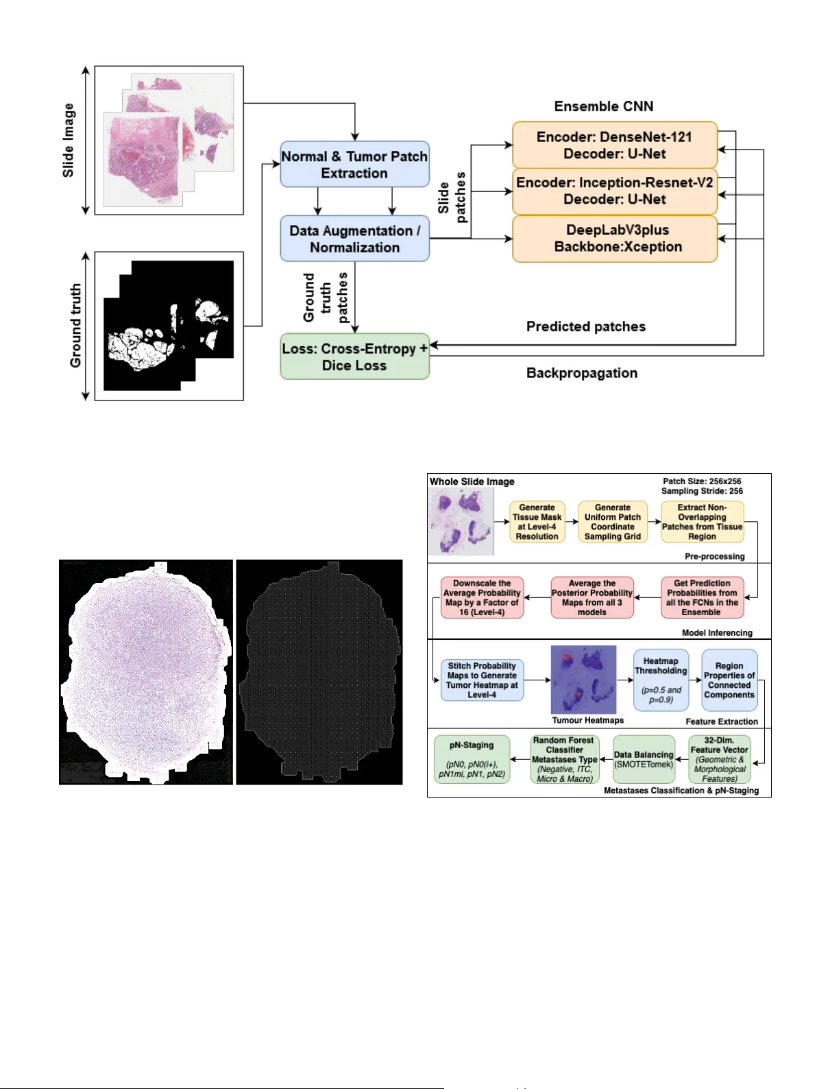
A Generalized Deep Learning Frame work for Whole-Slide Image Se gmentation and Analysis Mahendra Khened a,c , A vinash K ori a,c , Haran Rajkumar a,c , Balaji Sriniv asan b , Ganapathy Krishnamurthi a, ∗∗ a Department of Engineering Design, Indian Institute of T echnology Madr as, 600036 India b Department of Mechanical Engineering, Indian Institute of T ec hnology Madras, 600036 India c Authors contrib uted equally ABSTRA CT Histopathology tissue analysis is considered the gold standard in cancer diagnosis and prognosis. Whole slide imaging, i.e., the scanning and digitization of entire histology slides, are now being adopted across the world in pathology labs. T rained histopathologists can provide an accurate di- agnosis of biopsy specimens based on whole slide images (WSI). Ho wev er , given the lar ge size of these images and the increase in the number of potential cancer cases, an automated solution as an aid to histopathologists is highly desirable. In the recent past, deep learning-based techniques, namely , CNNs, have pro vided state of the art results in a wide variety of image analysis tasks, including anal- ysis of digitized slides. Howe ver , the size of images and variability in histopathology tasks makes it a challenge to develop an integrated framework for histopathology image analysis. W e propose a deep learning-based framew ork for histopathology tissue analysis. W e demonstrate the generaliz- ability of our framew ork, including training and inference, on several open-source datasets, which include CAMEL Y ON (breast cancer metastases), DigestPath (colon cancer), and P AIP (liv er can- cer) datasets. Our segmentation pipeline is an ensemble of DenseNet-121, Inception-ResNet-V2, and DeeplabV3Plus, where all the networks for each task were trained end to end. Our frame work provides segmentation maps gi ven a WSI. Our entire framew ork and related documentation are freely av ailable at GitHub and PyPi. 1. Introduction Histopathology is considered the gold standard for cancer di- agnosis (Gurcan et al., 2009; Salamat, 2010) and identification of prognostic and therapeutic targets. Early diagnosis of can- cer significantly increases the probability of surviv al (Hawk es, 2019). Unfortunately , pathological analysis is an arduous pro- cess that is di ffi cult, time-consuming, and requires in-depth knowledge. A study (Elmore et al., 2015) examining breast biopsies concordance among pathologists found that patholo- gists disagreed with each other on a diagnosis 24.7% of the time on average. This high rate of misdiagnosis stresses the need for the de velopment of computer -aided methods to aid the pathologists in histopathology . ∗∗ Corresponding author: e-mail: gankrish@iitm.ac.in (Ganapathy Krishnamurthi) Digital pathology is the method of digitizing the histology slides to produce high-resolution images (Jano wczyk and Mad- abhushi, 2016). Studies hav e been conducted on the collection, analysis and interpretation of digitized pathological slide im- ages (Gurcan et al., 2009). The increasing prev alence of whole slide imaging (WSI) technology that can scan the entire tissue slide at the subcellular level is making for conducting pathol- ogy analysis more viable (Madabhushi and Lee, 2016). Digital pathology’ s array of image analysis activities include identifi- cation and counting (e.g. mitotic e vents), segmentation (e.g. nuclei), and tissue di ff erentiation (e.g. cancerous vs. non- cancerous) (Janowczyk and Madabhushi, 2016; Nanthagopal and Rajamony, 2013; Guray and Sahin, 2006). Segmentation analysis helps in detecting and separating tumour cells from the normal cells (W ¨ ahlby et al., 2004; Xu et al., 2016). Seg- mentation of whole slide images is usually the precursor for performing v arious other do wnstream analyses such as classifi- cation and tumour burden estimation. 2 Automated whole slide image analysis is plagued by a myr- iad of challenges (T izhoosh and Pantano witz, 2018), namely: 1. Large dimensionality of whole slide images: A WSI dig- itizes a glass slide at a very high resolution of order 0.25 micrometres / pixel (which corresponds to 40X magnifica- tion on a microscope). A typical glass-slide of size 20mm x 15mm results in gigapixel image of size 80,000 x 60,000 pixels. 2. Insu ffi cient training samples: The main impediments to dev elopment and clinical implementation of deep learn- ing algorithms consist of su ffi ciently large, curated, and representativ e training data which includes expert la- belling which is a costly and time-consuming process (e.g., pathologist annotated data). Most clinical research groups currently hav e restricted access to data. The data is often based on small sample sizes with limited geographic variety which results in algorithms with limited utility and poor generalization. 3. Stain variability across laboratories: As the data is ac- quired from multiple sources, there e xists a lack of unifor- mity in staining protocol. Building a generalized frame- work that is inv ariant to stain pattern variability is chal- lenging. 4. Extraction of clinically relev ant features and information: Another major challenge is trying to extract features that are meaningful from a clinical point of view . Deep learn- ing does an excellent task of automatic feature extraction, but understanding these extracted features and extracting meaningful information from them is challenging. In this paper , a frame work developed for analyzing whole slide images of three di ff erent cancer sites is presented. The or - ganization of the paper is as follo ws. Prior work on histopathol- ogy image analysis using deep learning-based methods are dis- cussed in section 2. In section 3.2 the datasets used in this study are presented. Discussion on training and inference pipelines is provided in section 3.7 and 3.8 respecti vely . Experimental anal- ysis and comprehensi ve results are presented in section 4 and 5. Discussion of the results and conclusion of the proposed study with the possible course of research is provided in section 7. 2. Related work 2.1. Deep learning methods for histopathological image anal- ysis The adv ent of whole slide imaging scanners has enabled dig- itization of glass-slides at very high resolution. T ypical whole slide images are in the order of gigapix els and usually stored in multi-resolution p yramidal format. These slide images are suit- able for developing computer-aided diagnosis systems for au- tomating the pathologist workflo w and also with the av ailabil- ity of a large amount of data mak es them amenable for analysis with machine learning algorithms. In tumour pathology , nuclear morphology and cellular anatomy are often significant determinants of disease se verity . In order to make the diagnostic and grading task of tumour less subjectiv e, quantifiable features are deriv ed from the im- ages that correlate with the condition of the disease (Gurcan et al., 2009). For example, algorithms can be designed to de- tect in v asiv e tumours by first segmenting nuclei from the back- ground, quantifying a number of nuclear characteristics, such as size, shape and distribution, and comparing these character- istics with those of normal cells (Diamond et al., 2004). (Y u et al., 2016) predicted non-small cell lung cancer prognosis by applying classical machine learning algorithms that use engi- neered features deriv ed from pathology images. Feature engineered algorithms rely on a predetermined set of features to classify the tissue and can only classify the tissue as better as the features that di ff erentiate between them, and thus there is a limit to their e ffi ciency , e ven when there is a large amount of data available to refine the algorithm. Hence, there has been a significant shift in recent years towards the applica- tion of deep learning algorithms as they are known for its inher- ent ability to automatically deriv e features from its input data. T ypical deep learning-based approaches for whole slide image segmentation or classification are usually made by cropping the slide image into multiple small image patches and treating them as independent of each other during training and inference. Fur- thermore, to make an ov erall slide-level prediction or to gener- ate a heatmap of regions of interest, patch-lev el predictions are aggregated in a suitable manner . (Cruz-Roa et al., 2014) was one of the earlier w orks using this method that sho wed promis- ing results in detecting in vasi ve ductal breast carcinoma. Sev- eral studies hav e applied deep learning algorithms for various pathology tasks related to breast cancer , prostate biopsies, colon cancer , etc. Colorectal carcinoma is the third most common cancer in the world (Fleming et al., 2012). Majority of colorectal carcinoma are adenocarcinomas originating from epithelial cells (Hamil- ton, 2000). (Shapcott et al., 2019) discuss the application of deep learning methods for cell identification on TCGA data. (Kather et al., 2019) discuss the deep learning methods to pre- dict the clinical course of colorectal cancer patients based on histopathological images. (Bychkov et al., 2018) discuss the use of Long short-term memory (LSTM) (Gre ff et al., 2016) artificial recurrent neural network (RNN) architecture for esti- mating the patient risk score using spatial sequential memory . A revie w on WSI application for histopathological analysis of li ver diseases and for understanding liv er biology is gi ven by (Melo et al., 2019). They explore how WSI can enhance the ev aluation and quantification of sev eral histologic hepatic pa- rameters and help to identify various liver diseases with clinical implications. (Kiani et al., 2020) dev eloped a deep learning- based system to aid pathologists in di ff erentiating between two subtypes of primary liv er cancer , hepatocellular carcinoma and cholangiocarcinoma, on H&E stained whole slide images. (Lu and Daigle Jr, 2020) demonstrated the usefulness of extracting image features from hepatocellular carcinoma histopathologi- cal images using the pre-trained CNN models to reliably di ff er - entiate between normal and cancer samples. 2.2. Contributions A deep learning-based framew ork for segmentation and anal- ysis of whole slide images has been proposed. The framew ork 3 comprises of se gmentation network at its core along with no vel algorithms that utilize the segmentation to do pathological anal- yses such as metastasis classification and viable tumour b urden estimation. As discussed in section 1, challenges in whole slide image analysis are mainly due to their large size, variability in staining, and the limited amount of annotated data. In this work, the following contributions were proposed for addressing the aforementioned problems: • Ensemble segmentation model: The ensemble comprised of multiple FCN architectures, each independently trained on di ff erent subsets of the training data. During infer- ence, the ensemble generated the tumour probability map by averaging the posterior probability maps of all the FCNs. The ensemble approach showed superior segmen- tation performance when compared to its individual con- stituting FCNs. • T raining pipeline: The proposed approach divided the whole slide images into smaller sized image patches for the purpose of training FCN models. For the preparation of the training set, e ffi cient methodologies for sampling patches from the whole slide images were introduced. The problem of class-imbalance due to the limited number of representativ e patches from tumour regions in the whole slide images was addressed by employing o verlapping and ov ersampling techniques during patch extraction (random patch coordinate perturbation technique) alongside with various data augmentation schemes. • Inference pipeline: For e ffi ciently generating model in- ference on the entire whole slide image, a concept of generating patch coordinate sampling grid from the post- processed tissue mask was introduced. The sampling grid aided in the reduction of computational time by discard- ing non-tissue patches during the construction of the tu- mour probability heatmap. The patch-based segmentation of whole slide images introduced edge artefacts due to loss of neighbouring context information at patch borders, and this issue was addressed by proposing techniques to av- erage prediction probabilities at overlapping regions and making use of large patch size during inference. Apart from this, we also compute inference on multiple mod- els parallelly for ensemble calculation ov er patches rather than an entire image. • L ymph node metastases classification from whole slide images: A Random Forest-based ensemble classification algorithm was trained with hand-crafted features derived from the predicted tumour-probability maps. The class- imbalance in the training dataset was addressed by em- ploying strategies such as over -sampling (by synthetically generating under-presented class data points) and under- sampling (balance all classes by removing some noisy data points). • Uncertainty estimation: An e ffi cient patch-based uncer- tainty estimation frame work was dev eloped to estimate both data specific and model (parameter) specific uncer- tainties. T able 1: Summary of histopathological datasets used in this work. The test images were hidden by the competition or ganiz- ers and used only for leaderboard ev aluation. Dataset T rain set T est set < I mageS ize > Microns / pixel CAMEL YON16 270 129 100,000x100,000 0.25 CAMEL YON17 500 500 100,000x100,000 0.25 DigestPath 660 212 5,000x5,000 0.25 P AIP 50 40 50,000x50,000 0.5 T able 2: T umour size criteria for assigning metastasis type. Category Size Isolated tumour cells Single tumour cells or a cluster of tumour cells not larger than 0.2 mm or less than 200 cells Micro-metastasis Larger than 0.2 mm and / or con- taining more than 200 cells, but not larger than 2 mm Macro-metastasis Larger than 2 mm • Open-source Packaging: The proposed framew ork was packaged into an open-source GUI application for the ben- efit of researchers. The performance of the segmentation pipeline was bench- marked by v alidating it on whole slide images of three di ff erent cancer sites namely- breast lymph nodes, liv er and colon by par- ticipating in CAMEL YON (Litjens et al., 2018), DigestP ath (Li et al., 2019), and P AIP citeppaip challenges respecti vely . The framew ork is packaged into an open-source GUI application for the benefit of researchers 1 . 3. Materials and methods 3.1. Overview The Figure 1 provides an overvie w of the proposed deep learning based segmentation and downstream analyses frame- work for whole slide images corresponding to multiple di ff erent cancer sites. 3.2. Datasets used for this study The proposed frame work was v alidated on multiple open- source datasets which included CAMEL YON (Litjens et al., 2018), P AIP (Kim et al., 2019) and DigestPath (Li et al., 2019). T able 1 provides an o vervie w of the datasets used in this study . 3.2.1. CAMELY ON16 The CAMEL Y ON16 (Bejnordi et al., 2017) dataset com- prised of 399 whole slide images taken from two medical cen- tres in the Netherlands, out of which 159 whole slide images were metastases, and the remaining 240 were negati ve. Pathol- ogists exhausti vely annotated all the whole slide images with 1 https: // github .com / haranrk / DigiPathAI 4 Fig. 1: Deep learning based framew ork for segmentation and analysis of whole slide images. T able 3: Metastases type distribution in CAMEL YON17 train- ing set. Metastases (T raining Set) Negati ve ITC Micro Macro 318 35 64 88 metastases at the pixel lev el. In the CAMEL Y ON16 challenge, the 399 whole slide images were split into training and test- ing sets, comprising of 160 negati ve and 110 metastases whole slide images for training, 80 negati ve and 49 metastases whole slide images for testing. 3.2.2. CAMELY ON17 The CAMEL YON17(Bandi et al., 2018) dataset consisted of 1000 whole slide images taken from five medical centres in the Netherlands. In the CAMEL YON17 challenge, 500 whole slide images were allocated for training, and the remaining 500 whole slide images were allocated for testing. The training dataset of CAMEL Y ON17 included 318 negati ve whole slide images and 182 whole slide images with metastases. In CAME- L YON17 dataset, slide-lev el labels of metastases type were pro- vided for all the whole slide images, and exhausti ve pixel-le vel annotations were provided for 50 whole slide images. The slide-lev el labels were negati ve, Isolated T umor cells (ITC), micro-metastases and macro-metastases. T able 2 provides the size criteria for metastases type. The pN-stage labels were pro- vided for all the 100 patients in the training set and were based on the simplified rules provided in T able 4. The T able 3 pro- vides the metastases type distribution in CAMEL Y ON17 train- ing dataset. 3.2.3. P AIP The P AIP 2019 (Kim et al., 2019) dataset contains a total of 100 whole slide images scanned from liv er tissue samples. Each image has an av erage dimension of 50,000x50,000 pixels. T able 4: Pathologic lymph node classification (pN-stage) in CAMEL YON17 Challenge. pN-Stage Slide Labels pN0 No micro-metastases or macro-metastases or ITCs found. pN0(i + ) Only ITCs found. pN1mi Micro-metastases found, but no macro-metastases found. pN1 Metastases found in 1-3 lymph nodes, of which at least one is a macro-metastasis. pN2 Metastases found in 4-9 lymph nodes, of which at least one is a macro-metastasis. T able 5: List of features extracted for the purpose of predict- ing lymph node metastases type. Features were extracted after thresholding tumour probability heatmaps. For feature numbers 5, 6, 7, 8 and 9 the following statistics were computed- maxi- mum, mean, variance, sk ewness, and kurtosis. No. F eature description Threshold (p) 1 Largest tumour re gion’ s major axis length p = 0.9 & p = 0.5 2 Largest tumour re gion’ s area p = 0.5 3 Ratio of tumour region to tissue region p = 0.9 4 Count of non-zero pixels p = 0.9 5 T umour regions area p = 0.9 6 T umour regions perimeter p = 0.9 7 T umour regions eccentricity p = 0.9 8 T umour regions e xtent p = 0.9 9 T umour regions solidity p = 0.9 10 Mean of all region’ s mean confidence probability p = 0.9 11 Number of connected regions p = 0.9 5 Fig. 2: Whole slide image of a li ver tumour from the P AIP dataset. The green contour represents the viable tumour and the blue contour represents whole tumour . Annotations were made by expert pathologists. All the images were H&E stained, scanned at 20x magnifica- tion and prepared from a single centre, Seoul National Univer - sity Hospital. The dataset included pixel-lev el annotation of the viable tumour and whole tumour regions. It also provided the viable tumour burden metric for each image. T umour burden is defined as the ratio of the viable tumour region to the whole tumour region. The viable tumour region is defined as the cancerous region. The whole tumour area is defined as the outermost boundary enclosing all the dispersed viable tumour cell nests, tumour necrosis, and tumour capsule (Fig 2). Each tissue sample contains only one whole tumour region. This metric has applications in assessing the response rates of patients to cancer treatment. Out of the 100 images, 50 images were the publicly a v ailable training set, ten images were reserved for validation set that was made publicly av ailable after the challenge was completed, and the rest 40 images were the test set whose ground truth were not publicly av ailable. 3.2.4. DigestP ath DigestPath dataset consists of tissue sections collected dur- ing the examination of colonoscopy pathology to identify early- stage colon tumour cells. There are ten or more tissues sections in a single whole slide image for colonoscopy pathology re view . The challenge or ganisers selected one or tw o tissue sections in a whole slide image and pro vided images of these tissue sections along with their corresponding lesion annotations by patholo- gists in jpg format. On av erage, each tissue image was of size 5000x5000 pixels. The training dataset of DigestPath consists of 660 tissue images taken from 324 patients, in which 250 tis- sue images from 93 patients had lesions, and the remaining 410 tissue images from 231 patients had no lesions. The data was collected from multiple medical centres, especially from sev- eral small centres in developing countries. All the tissues sec- tions were H&E stained and scanned at 20x magnification. The testing dataset consisted of 212 tissue images from 152 patients. The challenge organisers released only the training set and the testing set were kept confidential. 3.3. Data pr e-pr ocessing 3.3.1. T issue mask generation In this step, the entire tissue region was segmented from the background glass region of the whole slide image. This step aided in prev enting unnecessary computations on non-tissue re- gions of the slide. An approximate tissue region boundary suf- fices, therefore the processing was done on a lo w resolution ver - sion of the whole slide image to further reduce computational costs. The RGB colour space of the low-resolution image was transformed to HSV (Hue-Saturation-V alue) colour space and Otsu’ s adapti ve thresholding (Otsu, 1979) was applied to the saturation component. Post thresholding, binary morphologi- cal operations were performed to facilitate proper extraction of patches at the small tissue regions and tissue borders. 3.3.2. T issue mask generation specific to CAMEL YON dataset In some of the CAMEL YON17 cases, the Otsu’ s threshold- ing failed because of the black regions in the whole slide image. Hence, before the application of image thresholding operation, the pre-processing in volv ed replacing black pix el regions in the whole slide image back-ground with white pixels and median blurring with a kernel of size 7x7 on the entire image. Median blur aided in the smoothing of the tissue regions and remov al of noise at the tissue bordering the glass-slide re gion while pre- serving the edges of the tissue. Figure 3 illustrates the pipeline for tissue mask generation with an example. 3.3.3. P atch coor dinate extraction Using the tissue mask, patches of the image were randomly extracted to make the training dataset. An equal number of tumorous and non-tumorous patches were extracted. A patch was considered tumorous if at least one pixel inside the patch was classified a tumor . The dimensions of the extracted patches were not fixed. Rather, they were a hyperparameter we experi- mented with. In this step, only the centers of the potential train- ing patches were extracted and stored. 3.3.4. Data augmentation T o increase the number of data points and to better gener- alize the models across various staining and acquisition pro- tocols, data augmentation schemes were proposed. Augmen- tations like “horizontal or vertical flip, ” “90-degree rotations”, and “Gaussian blurring” along with colour augmentation were performed. Colour augmentation included random changes to brightness, contrast, hue, and saturation with a maximum delta of 64.0 / 255, 0.75, 0.25, 0.04, respectiv ely . Additionally , in order to introduce some div ersity of patches extracted from the whole slide images during each training epoch, random coordinate perturbation was introduced. The random coordinate perturbation inv olved o ff setting the centre of the patch coordinates within a specified radius prior to the 6 Fig. 3: An illustration of the intermediate stages in the process of tissue mask generation from a whole slide image in CAME- L YON17 dataset. extraction from the whole slide image. The radius was fixed to be 128 pixels, and patches of size 256x256 pixels were ex- tracted from the highest resolution image. Since in the patch extraction phase, only the centers were extracted and stored, this augmentation could be applied on the fly during training. Post augmentation, the images were normalized. 3.4. Network ar chitectur e For the task of se gmentation of tumour regions from patches of the whole slide images fully conv olutional neural network (FCN) (Long et al., 2015) based architectures were used. A typical FCN based segmentation network comprises of an en- coder network, a decoder network and a pixel-wise classifica- tion layer . An encoder network comprises of a series of oper- ations (like con volution and pooling) that transforms the input (image) to a set of low resolution feature maps. The decoder network comprises of up-sampling or transposed conv olution followed by series of con volution operations that transform the low resolution encoder feature maps to the original input reso- lution feature maps for pixel-wise classification. The ensemble consisted of three encoder-decoder based FCN architectures. During inference, the predicted tumour poste- rior probability map from all the three models were av eraged to generate the ensemble model’ s final prediction. The ensemble comprised of the following FCN architectures: • U-Net (Ronneberger et al., 2015) with DenseNet-121 (Huang et al., 2017) as the backbone (encoder) pre-trained on ImageNet (Deng et al., 2009). The decoder comprised of the bi-linear up-sampling module follo wed by con v olu- tional layers. Features learnt in the down-sampling path of the encoder were concatenated with the features learnt in the up-sampling path using skip connection. • U-Net (Ronneberger et al., 2015) with Inception-ResNet- V2 (Szegedy et al., 2017) as the backbone (encoder) pre-trained on ImageNet (Deng et al., 2009). The Inception-ResNet-V2 (Szegedy et al., 2017) (also known as Inception-v4) integrates the features of the Inception ar - chitecture (Szegedy et al., 2015) and the ResNet architec- ture (He et al., 2016). • DeeplabV3Plus (Chen et al., 2018) with Xception (Chol- let, 2017) network as the backbone and pre-trained on P ASCAL VOC (Everingham et al., 2010). DeepLabV3 (Chen et al., 2017) was built to obtain multi-scale conte xt. This was done by using atrous conv olutions with di ff er- ent rates. DeeplabV3Plus e xtends this by having lo w-lev el features transported from the encoder to decoder . 3.5. Loss function T umour regions were represented by a minuscule proportion of pixels in whole slide images, thereby leading to class im- balance. This issue was circumvented by training the network to minimize a hybrid loss function. The hybrid loss function comprised of cross-entropy loss and a loss function based on the Dice overlap coe ffi cient. The Dice coe ffi cient is an ov erlap metric used for assessing the quality of segmentation maps. The 7 dice loss is a di ff erentiable function that approximates Dice- coe ffi cient and is defined using the predicted posterior proba- bility map and ground truth binary image as defined in 1. The cross-entropy loss is defined in 2. In the equations, p i and g i represent pairs of corresponding pixel values of predicted poste- rior probability and ground truth. N represents the total number of pixels. D L refers to dice loss and C L refers to cross-entropy loss. D L FG and D L BG represent the foreground pixels that cor- respond to the tumour regions and the background pixels that corresponded to non-tumour regions, respecti vely . DL = 1 − 2 P N i p i g i P N i p 2 i + P N i g 2 i (1) C L = N X i ( g i log ( p i ) + (1 − g i ) log (1 − p i ) ) (2) Lo s s = α ∗ C L + β ∗ D L BG + γ ∗ DL FG (3) The proposed loss was defined as a linear combination of the two-loss components as defined in 3. The neural networks were trained by minimizing the proposed loss function using AD AM optimizer ((Kingma and Ba, 2014)). The α, β, γ were empirically assigned to the individual loss components. The following configurations were set: α = 0 . 5 , β = 0 . 25 and γ = 0 . 25. 3.6. Uncertainty analysis Uncertainty estimation is essential in assessing unclear di- agnostic cases predicted by deep learning models. It helps pathologists to concentrate more on the uncertain regions for their analysis. (Begoli et al., 2019) argues the need for un- certainty analysis in machine-assisted medical decision-making system. There exist two main sources of uncertainty , namely (i) Aleatoric uncertainty and (ii) Epistemic uncertainty . Aleatoric uncertainty is uncertainty due to the data generation process it- self. In contrast, the uncertainty induced due to the model pa- rameters, which is the result of not estimating ideal model ar- chitectures or weights to fit the given data, is kno wn as epis- temic uncertainty (Kendall and Gal, 2017). Epistemic un- certainty can be approximated by using test time Bayesian dropouts as discussed in (Leibig et al., 2017), which estimates uncertainty by Montecarlo simulations with Bayesian dropout. In the proposed pipeline, aleatoric uncertainty for each model was estimated using test time augmentations, as introduced in (Gal and Ghahramani, 2016) 4. var al ( x , Φ i ) ≈ E t ∼ T T A [( Φ i ( x | w , t ) − E t ∼ T T A [ Φ i ( x | w , t )]) 2 ] (4) where Φ i ( x | w ) is the output of the neural network with weights w for input x and T T A denotes the set of possible test time data augmentations allowed. The proposed methodology for aleatoric uncertainty included the following augmentations- T T A ∈ { r otat ion , vertical f li p , hor izontal f li p } . For epistemic uncertainty , the div ersity of model architec- tures were used to calculate uncertainty 5. var e p ( p ( y | x , w )) ≈ E φ ∼{ Φ i } [( φ ( x | w ) − E φ ∼{ Φ i } [ φ ( x | w )]) 2 ] (5) where the likelihood distrib ution p ( y | x , w ) is a probabilistic model which generates outputs ( y ) for gi ven inputs ( x ) for some parameter setting ( w ) and Φ i indicates the trained model. 3.7. T raining pipeline Figure 4 illustrates the training strategy utilized for train- ing each of the models in the ensemble. The batches for training were generated with an equal number of tumour and non-tumour patches. This was done to prevent class imbal- ance or manifold shift issues and enforce proper training. All three models were trained independently , with di ff erent cross- validation folds of the data. The FCN architectures in the ensemble whose encoders were based on DenseNet-121 and Inception-ResNet-V2 made use of transfer learning by using ImageNet (Deng et al., 2009) pre-trained weights for their re- spectiv e encoders. In the case of DeeplabV3Plus, the model weights were pre-trained on PascalV OC (Everingham et al., 2010). For the network architectures with encoders based on DenseNet-121 and Inception-ResNet-V2, the encoder weights of the models were frozen for the first two epochs, and only the decoder weights were made trainable. For the remaining epochs, both the encoder and decoder parts were trained. The learning rate was decayed ev ery fe w epochs in a deterministic manner to allow for the model to gradually con verge. 3.8. Infer ence pipeline The pre-processing step in the inference pipeline included segmentation of tissue region from the whole slide image (re- fer 3.3.1). In order to facilitate extraction of patches from the whole slide image within the tissue mask region, a uniform patch-coordinate sampling grid was generated at a lower res- olution, as sho wn in Figure 5. Each point in the patch sampling grid was re-scaled by a factor to map to the coordinate space corresponding to the whole slide image at its highest resolution. From these scaled coordinate points as the centre, fixed-size high-resolution image patches were extracted from the whole slide image for feeding the trained segmentation model’ s in- put. The sampling stride was defined as the spacing between consecutiv e points in the patch sampling grid. The patch size and the sampling stride controlled the overlap between consec- utiv e extracted patches from the whole slide image. The main drawback of patch-based segmentation method for whole slide image was that the smaller patch sizes could not capture wider context of the neighbourhood region. Moreov er , stitching of the segmented patches introduced boundary artefacts (blockish appearance) in the tumour probability heatmaps. The gener- ated heatmaps were smooth when the inference was done on ov erlapping patches with larger patch-size and averaging the prediction probabilities at the overlapping regions. The ex- perimental observation suggested that 50% o verlap between consecutiv e neighbouring patches was the optimal choice as it ensured that a particular pixel in a whole slide image was seen at most 4-times during the heatmap generation. Ho w- ev er , this approach increased the inference time by a factor of 4. Also, during inference, increasing the patch size by a factor of 4 (1024x1024) when compared to the patch size used during training (256x256) improv ed the quality of generated heatmaps. 3.9. pN-staging pipeline for CAMEL YON17 dataset Figure 6 illustrates the complete pipeline dev eloped for pN- staging of CAMEL Y ON17 dataset. The pipeline comprises four blocks as described below: 8 Fig. 4: Overvie w of the tumour segmentation training pipeline. Fig. 5: (Left to Right) An illustration of the tissue mask ov er- layed on a small region of the whole slide image at low reso- lution (level-4), here the white region corresponds to the tissue mask; An illustration of the generated uniform patch coordinate sampling grid, here the points on the image act as centres from which high-resolution image patches were extracted from the whole slide image. Fig. 6: Overvie w of the steps in v olved in the pN-staging pipeline dev eloped for CAMEL YON17 dataset. • Pre-processing: The tissue regions in the whole slide im- ages were detected for patch extraction. • Heatmap generation: The extracted patches from the whole slide images were passed through the inference pipeline to generate the do wn-scaled version of the tumour probability heatmaps. • Feature extraction: The heatmaps were binarized by 9 thresholding at 0.5 and 0.9 probabilities, and at each of these thresholds, the connected components were ex- tracted, and region properties were measured using scikit- image (van der W alt et al., 2014) library . Thirty-tw o geometric and morphological features from the probable metastases regions were computed. • Data balancing: In order to handle the class imbalance problem, one of the techniques proposed in the literature is o versampling by synthetically generating minority class samples using SMO TE algorithm (Chawla et al., 2002). Howe ver , this method can introduce noisy samples when the interpolated ne w samples lie between mar ginal outliers and inliers. This problem is usually addressed by remov- ing noisy samples by using under-sampling techniques like T omek’ s link (T omek, 1976) or nearest-neighbours. SMO TET omek (Batista et al., 2004) algorithm was em- ployed for balancing the training data. SMOTET omek al- gorithm is a combination of SMO TE and T omek’ s link per- formed consecutiv ely . • Classification: The pN-stage was assigned to the patient based on all the a v ailable lymph-node whole slide images, taking into account their individual metastases type (T a- ble 2). For predicting the metastases type, an ensemble of Random Forest classifiers (Liaw et al., 2002) was trained using the extracted features. 3.10. T umour bur den estimation for P AIP dataset The tumour burden computation requires the segmentation of viable tumour and whole tumour regions in the whole slide im- age of the liv er cancer tissue. The viable tumour region was seg- mented using the proposed deep learning-based segmentation network. Howe ver , it was observed that training the same seg- mentation network for whole tumour region gav e sub-optimal results. Hence, a heuristic method was adopted to approximate the whole tumour region from viable tumour re gion. The tumour burden estimation algorithm consisted of the fol- lowing steps: • Segment the viable tumour re gion from image • Apply morphological operation to remove false positi ves and fill holes • Find the smallest con vex hull containing the entire viable tumour region • Estimate the tissue mask, as discussed in 3.3.1. • The whole tumour region is approximated to be the inter- section of the con ve x hull and tissue mask region. • The tumour burden is calculated by taking the ratio be- tween the area of the viable and whole tumour regions 4. Experimental analysis In this section, the e ff ectiv eness of the proposed methodolo- gies for segmentation and classification models are experimen- tally analyzed. The neural networks were implemented using T ensorFlow-K eras ((Abadi et al., 2016)) deep learning frame- work. The experiments were run on multiple desktop comput- ers with NVIDIA T itan-V GPU with 12 GB RAM, Intel Core i7-4930K 6-core CPUs @ 3.40GHz, and 48GB RAM. 4.1. Lesion detection analysis on CAMELY ON16 dataset In this section, some of the techniques specific to CAME- L YON dataset pre-processing are detailed, and discussion on the performance of various FCN architectures and ensemble configurations for lesion detection on the CAMEL YON16 test dataset (n = 139) are provided. 4.1.1. FR OC evaluation scor e One of the metrics used in CAMEL YON16 challenge for lesion-based ev aluation is free-response recei ver operating characteristic (FR OC) curve. The FR OC curv e is defined as the plot of sensitivity versus the average number of false-positi ves per image. The CAMEL YON16 challenge testing dataset was used for evaluating the performance of the proposed algorithms for lesion detection / localization. The detection / localization performance was summarized using Free Response Operating Characteristic (FR OC) curves. This was similar to R OC analy- sis, except that the false positiv e rate on the x-axis is replaced by the av erage number of f alse positi ves per whole slide image. The following guidelines were followed for lesion detection in CAMEL YON16 challenge. • If the position of the detected region was inside the anno- tated ground truth lesion it was considered a true positi ve • If a single ground-truth region had sev eral findings, they were counted as a single true positi ve finding, and none of them were counted as false positi ves • All detections which were not within a reasonable distance of the annotations of ground truth were counted as false positiv es • The final FR OC score was defined as the a verage sensiti v- ity at six predefined false positives: 1 / 4, 1 / 2, 1, 2, 4 and 8 FPs per whole slide image 4.1.2. Dataset pr eparation specific to CAMEL YON dataset For training the ensemble se gmentation model for lesion seg- mentation, training sets of both CAMEL YON16 and CAME- L YON17 dataset which had pixel-le vel annotations for the whole slide images were used. As noted by the challenge or- ganizers, some of the whole slide images were not exhausti vely annotated in the CAMEL Y ON16 training set; such slides were excluded in training set preparation. So, in total, 628 whole slide images for training were utilized (250 whole slide im- ages from CAMEL YON16 and 378 from CAMEL YON17). A three-fold stratified cross-v alidation split of the training set was done to maximize the utilization of the limited number of whole 10 T able 6: Count of the tumour and non-tumour patches in each of the three cross-validation folds. Patch label No. of patch coordinates Fold-0 F old-1 Fold-2 T raining Non-T umour 1,87,034 1,96,094 1,90,424 T raining T umour 1,84,467 1,94,709 1,87,440 V alidation Non-T umour 99,742 90,682 96,352 V alidation T umour 99,786 89,544 96,813 Fig. 7: The figure illustrates the overlap-stitch inference pipeline used in Ensemble-B configuration. slide images. The stratification ensured that the ratio of nega- tiv e to metastases was maintained in all the three folds. From 628 whole slide images, 5,71,029 coordinates whose patches corresponded to regions from the tumour and non-tumour tis- sue regions were randomly sampled. A patch extracted from a whole slide image was labelled as a tumour patch if it had non-zero pixels labelled as tumour pixels in the pathologist’ s manual annotation. Further , these extracted patch coordinates were distrib uted into their respectiv e cross-v alidation folds. T a- ble 6 shows the distrib ution of the split in each of the folds. 4.1.3. T raining and infer ence configuration of ensemble FCN models The following tw o ensemble configurations were proposed: • Ensemble-A: Comprised of the three di ff erent FCN ar- chitectures, as described in section 3.7. The inference pipeline made use of patch size of 256 and extracted non- ov erlapping patches. • Ensemble-B: Comprised of three replicated versions of a single FCN architecture. The inference pipeline made use of a patch size of 1024 with a 50% o verlap between neigh- bouring patches, as illustrated in Figure 7. In both the ensemble configurations, each model in the en- semble was trained with one of the 3-fold cross-validation splits. All the models made use of pre-trained weights with the fine-tuning procedure, as described in section 3.7. The models were trained for ten epochs with a batch size of 32. 4.1.4. Lesion detection performance of Ensemble-A Experimental results suggested that DenseNet-121 architec- ture had higher sensitivity and reduced false positives when (a) (b) Fig. 8: (a) A whole slide image from CAMEL Y ON16 test set, (b) T umour ground truth ov erlayed on the whole slide image. Fig. 9: The figure shows the heatmaps ov erlayed on the whole slide image by FCN models in Ensemble-A configuration. (Left to Right): DenseNet-121 FCN, Inception-ResNet-V2 FCN, DeepLabV3plus, Ensemble, (Patch Size: 256x256, Sampling Stride: 256 pixels). compared to other FCNs in the ensemble configuration. It was also observed that Ensemble-A showed a significant di ff erence in the FR OC score compared to its constituents. The reason for this significant boost in the performance of Ensemble-A could be attributed to the e ff ect of av eraging the heatmaps from multi- ple FCN models, thereby lowering the probabilities of uncertain or less confident regions and hence eliminating the false posi- tiv es. Figure 9 illustrates the heatmaps generated by Ensemble- A and its constituent FCN models on a CAMEL Y ON16 test case (refer Figure 8). T able 7: FROC scores achiev ed on CAMEL Y ON16 test set (n = 139) by FCN models in Ensemble-A configuration. Note the abbre viations: IRF - Inception-ResNet-V2 FCN, DF- DenseNet-121 FCN, DL- DeepLabV3Plus, FP- false positi ves. A vg. FPs / Slide Sensitivity IRF(Fold-0) DF(Fold-1) DL(Fold-2) Ensemble-A 0.25 0.5 0.59 0.03 0.77 0.5 0.59 0.65 0.06 0.8 1 0.69 0.72 0.2 0.83 2 0.77 0.79 0.48 0.84 4 0.8 0.83 0.64 0.86 8 0.82 0.85 0.77 0.86 FR OC Score 0.69 0.74 0.36 0.83 11 Fig. 10: The figure shows the heatmap ov erlayed on the whole slide image by FCN models in Ensemble-B configuration. (Left to Right): 3 DenseNet-121 FCN models trained on cross- validation folds: 1, 0 and 2 respectively and Ensemble-B, (Patch Size: 1024x1024, Sampling Stride: 512 pixels). It can be seen from the heatmaps that the models struggled (relati vely high posterior probability values at non-tumour regions) at ex- tended regions from tissue boundaries. 4.1.5. Lesion detection performance of Ensemble-B Since there was a marginal di ff erence in FROC scores be- tween various ensemble configurations (T able 9); hence in the interest of minimizing the computation time, Ensemble-A con- figuration was preferred with patch-size of 256x256 and sam- pling stride set to 256 (non-ov erlapping patch acquisition) for running inference on CAMEL YON17 testing dataset (n = 500). T able 8: FROC scores achiev ed on CAMEL Y ON16 test set (n = 139) by FCN models in Ensemble-B configuration (patch size- 1024 and sampling stride- 512). Note the abbreviations: DF-DenseNet-121 FCN, FP-false positi ves, F-F old. A vg. FPs / Slide Sensitivity DF (F-0) DF (F-1) DF (F-2) Ensemble-B 0.25 0.56 0.56 0.61 0.77 0.5 0.65 0.63 0.69 0.84 1 0.71 0.70 0.76 0.85 2 0.77 0.75 0.81 0.88 4 0.82 0.80 0.84 0.88 8 0.86 0.86 0.88 0.89 FR OC Score 0.73 0.72 0.77 0.85 4.2. L ymph-node metastases type classification analysis on CAMELY ON17 dataset In this section, the experimental analysis of the classification model for lymph node metastases types is presented. T able 9: The table shows the FROC scores on CAMEL YON16 test set (n = 139) for v arious configurations of model, patch-size, and sampling-stride. Model Patch size Sampling stride FR OC score Ensemble-A 256 256 0.83 Ensemble-B 256 256 0.84 Ensemble-B 1024 1024 0.86 Ensemble-B 1024 512 0.85 T able 10: Metastases type distribution in CAMEL YON17 train set and validation set. Dataset No. of whole slide images per each metastasis type Negati ve ITC Micro Macro T otal T rain set 100 26 35 44 215 V alidation set 98 35 64 88 285 4.2.1. Cohen’ s kappa evaluation scor e Cohen’ s kappa (Fleiss and Cohen, 1973) is a statistic that measures the inter-rater reliability for categorical variables. In CAMEL YON17 challenge for e valuating pN-staging of the pa- tients, the metric used was Cohen’ s kappa with fiv e classes and quadratic weights. The kappa metric ranges from -1 to + 1, where 1 represented perfect agreement with the raters, and 0 represented the amount of agreement that can be expected by random chance and, a negati ve value represented lo wer than chance agreement. 4.2.2. Dataset pr eparation The CAMEL YON17 training dataset had 100 patients, and each patient had fi ve whole slide images with their correspond- ing metastases labels (total 500 slide images). The training dataset comprising of 100 patients were split into 43 patients as a train set and the remaining 57 patients as a validation set. The split ensured that the patients in the train set had at least one whole slide image with pixel-lev el annotation. The T a- ble 10 shows the distribution of whole slide images in terms of metastases type between train and validation sets; the pro- posed split strategy ensured that the distribution of metastases type between the two splits was similar . 4.2.3. P erformance of Random F or est classifier without data balancing The tumour probability heatmaps for all the 500 whole slide images were generated using Ensemble-A configuration (sec- tion 4.1.3), and from the heatmaps, all the features listed in T a- ble 5 were extracted. Post generation of features, the training set was cleaned by removing some of the outlier points. The outliers were detected based on threshold-based heuristics like the presence of significantly large tumour false-positi ve regions in negati ve cases etc. For the purpose of classifier selection, feature elimination and hyper-parameter tuning, the classifiers were initially trained on the train set (n = 215) and later validated on the held-out v alidation set (n = 285). Experimentation on var - ious classifiers showed that the optimal performance in terms of classification accuracy (90.18%) and Cohen’ s kappa score (0.9164) on held-out validation set was achieved with Random Forest classifier with 100 trees. From T able 10, it can be ob- served that the data distribution was highly class imbalanced, with negati ve cases being the majority class and ITC cases be- ing the minority class. This lead to misclassifications between ITC and negati ve cases, as e vident in the confusion matrix. Further experimentation was performed by training another Random Forest classifier on the complete training set (n = 500) 12 T able 11: The table provides the validation results of the four Random Forest classifiers, each trained on di ff erent subsets of the training data. Note: For the models RF-PI and RF-PB, held- out validation existed, whereas, for the other two models, it was not av ailable as it was trained on the entire training set, and hence N.A (not applicable) is mentioned in the table. For all the models, 5-fold cross-validation accuracy was estimated on their respectiv e training sets. These values are provided as mean (standard deviation). Accuracy (%) Classifier 5-fold CV V alidation set RF-PI 87 (0.06) 90.18 RF-PB 92 (0.03) 87.02 RF-CI 89.89 (0.03) N.A RF-CB 94.83 (0.02) N.A T able 12: Segmentation results on the held-out validation set (n = 25) of DigestPath dataset. Model Dice DeepLabV3Plus 0.81 DenseNet-121 FCN 0.84 Inception-ResNet-V2 FCN 0.84 Ensemble 0.86 in order to maximize the utilization of training points. The fi ve- fold cross-validation showed an average accuracy score of 90%, and its performance was similar to the model trained on train set (n = 215). The above two trained models are referred to as RF-PI and RF-CI (Random Forest classifiers trained on the partial and complete training set with imbalanced class data, respecti vely). 4.2.4. P erformance of Random F orest classifier after data bal- ancing The train set (n = 215) split and the complete training set (n = 500) were separately balanced using SMOTET omek algo- rithm and two Random Forest classifiers were trained using these two balanced datasets. The two trained models are re- ferred to as RF-PB and RF-CB (Random Forest classifiers trained on P artial and Complete training set, which are Bal- anced data, respectiv ely). T able 11 provides the results of the validation study performed on all four models. It was observed that post data balancing of the training dataset, the 5-fold cross- validation accurac y scores improv ed by a margin of 5%. 4.3. T umour segmentation analysis on Dig estP ath dataset In this section, details specific to the training and inference strategies on DigestPath dataset are presented. Out of 660 tis- sue images from DigestPath training set, 635 images were used for training, and the remaining images were used as held-out validation set (n = 25) for model selection and hyperparameter tuning. The training set (n = 635) was split further into three- fold cross-validation sets; each set of data was used to train the individual models in the ensemble. A total of 80,000 patches from the entire training data were extracted, and each model was trained on patch size of 256x256 and a batch size of 32. Fig. 11: An illustration of the se gmentation results on a sample from DigestPath dataset. (Clockwise from top left) Whole slide image of H&E stained colon cancer tissue; Pathologist anno- tated ground truth of the tumour ov erlayed on the whole slide image (green region indicates the tumour); Segmentation map ov erlayed on the whole slide image (probability map thresh- olded at 0.5); Heatmap of T umour probability . The detected false positi ves are circled (d). 13 Fig. 12: An illustration of the segmentation results on a sam- ple from P AIP dataset. (Clockwise from top left) Whole slide image of H&E stained liv er cancer tissue; Pathologist anno- tated ground truth of the tumour overlayed on whole slide im- age (blue region indicates the tumour); Segmentation map over - layed on whole slide image (probability map thresholded at 0.5); Heatmap of T umour probability . The detected false posi- tiv es are circled (d). The model inference procedure inv olved extraction of patches of size 256x256 with 50% overlap between adjacent patches in batches of 32. In order to generate the binary segmentation map, the predicted tumour probability map was thresholded at 0.5. Figure 11 illustrates an example of the segmentation map generated by the proposed ensemble model. The trained mod- els were tested on held out validation set (n = 25), and the corre- sponding results are tabulated in T able 12. 4.4. T umour segmentation analysis on P AIP dataset In this section, details specific to the training and inference strategies on P AIP dataset are presented. The tissue mask gen- eration (as detailed in 3.3.1) incorporated the post-processing step of closing morphological operation with a kernel size of 20, followed by an opening operation with a kernel size of 5 and a final dilation operation with a kernel size of 20. The train- ing data set (n = 50) was split into fiv e-fold cross-validation and out of these fi ve-folds only three of them were used for training the models of the ensemble. The data was split into fiv e-folds as opposed to three-folds to ensure that each training set had at least 40 samples. A total of 200,000 patches from the entire training dataset were extracted with equal contributions from each training sample. The models were trained with a patch size of 256 and a batch size of 32. The model inference pro- T able 13: Segmentation results on the validation set (n = 10) of P AIP dataset. Model Jaccard Score DeepLabV3Plus 0.681786 Inception-ResNet-V2 FCN 0.685771 DenseNet-121 FCN 0.679107 Ensemble 0.701621 (a) (b) (c) Fig. 13: (Left to Right) V iable tumour prediction; Whole tu- mour prediction; Pathologist annotated whole tumour ground truth cedure inv olved extraction of non-overlapping patches of size 1024x1024 in batches of 16. For the generation of segmentation maps, the generated tumour probability maps were thresholded at 0.5. The threshold was decided based on the experimental analysis for a range of threshold values on the v alidation set (n = 10). The optimal threshold value was found to be 0.5. It was observed that lo wer thresholds resulted in false positiv es in samples and higher thresholds led to under-segmentation. Fig- ure 12 illustrates an example of the segmentation map gener- ated by the proposed ensemble configuration. The performance of the trained models on the validation set (n = 10) released by the challenge organisers is tab ulated in T able 13. 4.5. V iable tumour bur den analysis on P AIP dataset Fig. 13 shows the results obtained using the proposed methodology described in section 3.10. In (a) the predicted whole tumour segmentation was similar to pathologist provided ground truth of whole tumour region and most of the samples in the dataset fell into this cate gory . The proposed method- 14 Fig. 14: (a) Colon cancer tissue sample from DigestPath dataset, (b) Pathologist annotation of tumour ov erlayed on whole slide image, (c) T umour probability heatmaps overlayed on the whole slide image and, (d) Aleatoric uncertainty maps. ology for the whole tumour region failed in following cases where - (b) the predicted viable tumour regions were scattered into small discrete disjoint re gions which were distant from the most prominent viable tumour region and (c) the whole tumour region was larger than the con vex hull of the viable tumour re- gion. 4.6. Uncertainty analysis In this section, the demonstration and interpretation of the proposed uncertainty analysis on the DigestPath dataset. Anal- ysis of the P AIP 2019 and CAMEL Y ON are present in the sup- plementary section. Fig. 15 provides an illustration of aleatoric and epistemic uncertainty analysis on a held-out test case from the DigestPath dataset. The proposed patch-based method for aleatoric uncertainty estimated high uncertainty v alues inside tumour regions because of prev alent loss of neighbouring con- text information at patch borders; hence aleatoric uncertainty estimation necessitates the analysis to be conducted on a larger contiguous region of a whole slide image. The proposed un- certainty analysis was done with a patch size of 256 × 256 be- cause of computational constraints. In Figure 15 (4)(d) illus- trates epistemic uncertainty maps, where the uncertain regions corresponded to the boundary surrounding the tumour tissue. In Figure 15 (5)(d) illustrates the map of combined uncertainties (av erage of aleatoric uncertainties for all the three models along with epistemic uncertainty across the three models). In Figure 15 (4,5)(c), indicates that the ensemble prediction reduced the number of false positi ves, thereby increasing ov erall Dice score to 0.94, which is about 0.04-0.06 improvement in Dice score when compared to the individual models. 4.7. CAMELY ON uncertainty maps Figure 15 provides an illustration of aleatoric and epistemic uncertainty analysis on a held-out test case from the CAME- L YON dataset. 5. Challenge results 5.1. P erformance evaluation on CAMEL YON17 c hallenge On the CAMEL YON17 testing dataset (n = 500) the ensem- ble strategy was employed by combining the predictions from all the four trained Random Forest classifiers. The ensembling was based on the majority voting principle, and in case of a tie, the higher metastases category was selected. The ensem- ble model is referred to as RF-Ensemble. T able 14 compares T able 14: Comparison of the proposed with other published approaches for automated pN-Staging in CAMEL Y ON17 chal- lenge. The score reported in the table is from the open public leader board of CAMEL YON17 challenge. The proposed ap- proach (RF-Ensemble) stood rank-3 on the leader-board (Ac- cessed on 31-Dec-2019). The table additionally provides the performance of individual Random Forest classifiers in the en- semble and RF-Ensemble classifier . Method Cohen Kappa Score Rank (Lee et al., 2019) 0.9570 1 (Pinchaud, 2019) 0.9386 2 Proposed (RF-Ensemble) 0.9090 3 Proposed (RF-PI) 0.8971 12 Proposed (RF-PB) 0.9027 9 Proposed (RF-CI) 0.8889 18 Proposed (RF-CB) 0.9057 6 T able 15: T op four entries in DigestPath-2019 challenge. T eams Dice kuanguang 0.807 zju realdoctor 0.792 TIA Lab 0.787 Proposed 0.782 the results of the proposed ensemble approach with other pub- lished approaches on CAMEL YON17 testing dataset (n = 500). The proposed ensemble strategy gave Cohen’ s kappa score of 0.9090. 5.2. P erformance evaluation on Dig estP ath 2019 challeng e T able 15 compares the results of the proposed with other ap- proaches on DigestPath-2019 testing dataset (n = 212). The pro- posed approach obtained a Dice score of 0.78 on the test set. 5.3. P erformance evaluation on P AIP 2019 challenge T able 16 compares the results of the proposed with other ap- proaches on P AIP-2019 testing dataset (n = 40). The challenge comprised of two tasks, described as follo ws- • T ask 1: Liver cancer segmentation performance was ev al- uated using av erage Jaccard index. • T ask 2: V iable tumour burden estimation was ev aluated as the av erage of products of absolute accuracy and corre- sponding T ask 1 score (Jaccard inde x) for each of the cases in the test set. For T ask 1, all the participants utilized deep learning-based methods for segmentation of viable tumour , albeit with di ff erent CNN architectures. For T ask 2, all the participants used deep learning-based methods for segmentation of the whole tumour . The proposed con v ex hull based approximation method showed comparable performance with deep learning-based methods. 15 (a) (1) DenseNet-121 FCN model predictions with aleatoric uncertainty (Dice = 0.91). (b) (2) Inception-ResNet-V2 FCN model predictions with aleatoric uncertainty (Dice = 0.89) (c) (3) DeepLabv3Plus model predictions with aleatoric uncertainty (Dice = 0.88). (d) (4) Ensemble model predictions with epistemic uncertainty (Dice = 0.94). (e) (5) Ensemble model predictions with combined uncertainty (Dice = 0.94). Fig. 15: In the figure for 1-5 (a) Whole slide image of H&E stained lymph node section from CAMEL Y ON dataset, (b) Pathologist annotation of tumour overlayed on whole slide image, (c) T umour probability heatmaps overlayed on the whole slide image and, (d) Corresponding uncertainty analysis maps. 16 T able 16: T op fiv e entries of P AIP 2019. T ask 1 corresponds to V iable tumour segmentation and T ask 2 corresponds to V iable tumour burden estimation. Note: FNLCR: Frederick National Laboratory for Cancer Research. T eam T ask 1 T ask 2 FNLCR 0.789 0.752 Sichuan Univ ersity 0.777 N A Proposed 0.750 0.6337 Alibaba 0.672 0.6199 Sejong Univ ersity 0.665 0.6330 Fig. 16: User interface of the whole slide image analysis soft- ware. 6. Open source contrib ution An open-source application (Rajkumar et al., 2019) on top of the proposed segmentation pipeline was dev eloped and re- leased. The application (Figure 16) can load whole slide im- ages, run the segmentation algorithm, and calculate the uncer- tainties. The software is modular making it easy for researchers to easily add their own segmentation pipelines or extend it’ s functionality . an API with which researchers can utilize the segmentation pipeline within their applications. Conv ersely , the application’ s modular structure allows for researchers to test their segmen- tation pipeline with the application’ s GUI as well. The slide viewer was b uilt using OpenSlide (Goode et al., 2013) and OpenSeadragon (V andecreme et al.). 7. Discussion and conclusions An automated end-to-end deep learning-based frame work for segmentation and downstream analysis of whole slide im- ages was dev eloped. The proposed framew ork showed state- of-the-art results on three publicly available histopathology image analysis challenges, namely , CAMEL YON, P AIP 2019 and DigestP ath 2019. The problem of segmentation of gi- gapixel whole slide images was approached using the divide- and-conquer strategy by dividing the large image into com- putationally feasible patch sizes and running segmentation al- gorithms on patches and stitching segmented patches to gen- erate the segmentation of the entire whole slide image. The patches were segmented using an ensemble of FCNs, which are encoder-decoder based architectures employed for generating dense pixel-lev el classification. The encoders in the proposed FCNs were some of the state-of-the-art CNNs used for natu- ral image analysis tasks, and the decoders were a learnable up- sampling module to generate dense predictions. The proposed segmentation framew ork was an ensemble comprising of mul- tiple FCN architectures, each independently trained on di ff er- ent subsets of the training data. The ensemble generated the tumour probability map by averaging the posterior probability maps of all the FCNs. The ensemble approach showed supe- rior segmentation performance when compared to its individ- ual constituting FCNs. The patch-based segmentation methods for large-sized images su ff er from loss of neighbouring context information at patch borders. This issue was addressed during inference by proposing- (i) to use patch size larger than that used during training and (ii) av eraging overlapping patch re- gion’ s posterior probability maps while stitching tumour prob- ability maps for the entire whole slide image. In addition to the generation of tumour probability heatmaps, a methodology for generating uncertainty maps based on model and data vari- ability was also incorporated into the framew ork. These uncer- tainty maps would assist in better interpretation by pathologists and fine-tuning the model with uncertain regions. Further research can be done in the design of e ffi cient and multi-resolution FCN architectures for capturing multi- resolution information from whole slide images (Graham et al., 2019). The proposed experimental analysis on transfer learn- ing showed that pre-training models with di ff erent histopathol- 17 ogy datasets could act as good starting points for training mod- els were pathology datasets are limited. Post-processing tech- niques could be one of the directions to improv e the predicted whole slide image’ s tumour segmentation; techniques such as patch-based conditional random fields (Kr ¨ ahenb ¨ uhl and K oltun, 2011; Li and Ping, 2018) could be employed to refine the pre- dicted segmentation masks rather than employing hardcoded threshold values. The segmentation of whole slide images is usually the pri- mary step for many analysis tasks such as metastases classifi- cation and estimation of tumour burden. In this regard, an au- tomated pipeline for lymph node metastases classification and pN-staging was dev eloped. For the task of lymph node metas- tases classification, an ensemble of multiple Random Forest classifiers was proposed, and each classifier was trained on dif- ferent subsets of the training data. The training data was pre- pared by extracting features based on the pathologist’ s view- point from the tumour probability maps. Additionally , incorpo- rating synthetically generated training samples into the training data demonstrated its e ffi cacy in addressing class imbalanced datasets for such classification tasks. The proposed method for viable tumour burden estimation from whole slide images of liver cancer utilized an empirical method for estimating the whole tumour region from the pre- dicted viable tumour region. The whole tumour region was pro- posed to approximate a con vex hull around the viable tumour region. This approximation performed on par with other deep learning-based segmentation approaches and was also compu- tationally inexpensi ve. The proposed method could be refined further by incorporating learning-based methods. For example, the conv ex hull output could be used as an initial point for active contours-based models (Kass et al., 1988) for correcting whole tumour region se gmentation. References Abadi, M., Agarwal, A., Barham, P ., Brevdo, E., Chen, Z., Citro, C., Cor- rado, G.S., Davis, A., Dean, J., Devin, M., et al., 2016. T ensorflow: Large- scale machine learning on heterogeneous distributed systems. arXiv preprint arXiv:1603.04467 . Bandi, P ., Geessink, O., Manson, Q., V an Dijk, M., Balkenhol, M., Hermsen, M., Bejnordi, B.E., Lee, B., Paeng, K., Zhong, A., et al., 2018. From detec- tion of individual metastases to classification of lymph node status at the pa- tient level: the camelyon17 challenge. IEEE transactions on medical imag- ing 38, 550–560. Batista, G.E., Prati, R.C., Monard, M.C., 2004. A study of the behavior of sev- eral methods for balancing machine learning training data. ACM SIGKDD explorations ne wsletter 6, 20–29. Begoli, E., Bhattacharya, T ., Kusnezo v , D., 2019. The need for uncertainty quantification in machine-assisted medical decision making. Nature Ma- chine Intelligence 1, 20. Bejnordi, B.E., V eta, M., V an Diest, P .J., V an Ginneken, B., Karssemeijer, N., Litjens, G., V an Der Laak, J.A., Hermsen, M., Manson, Q.F ., Balkenhol, M., et al., 2017. Diagnostic assessment of deep learning algorithms for detection of lymph node metastases in women with breast cancer. Jama 318, 2199– 2210. Bychkov , D., Linder , N., Turkki, R., Nordling, S., Ko vanen, P .E., V errill, C., W alliander, M., Lundin, M., Haglund, C., Lundin, J., 2018. Deep learning based tissue analysis predicts outcome in colorectal cancer . Scientific reports 8, 3395. Chawla, N.V ., Bowyer , K.W ., Hall, L.O., Ke gelmeyer , W .P ., 2002. Smote: synthetic minority ov er-sampling technique. Journal of artificial intelligence research 16, 321–357. Chen, L.C., Papandreou, G., Schro ff , F ., Adam, H., 2017. Rethinking atrous con volution for semantic image segmentation. arXiv preprint arXiv:1706.05587 . Chen, L.C., Zhu, Y ., Papandreou, G., Schro ff , F ., Adam, H., 2018. Encoder- decoder with atrous separable con volution for semantic image segmentation, in: Proceedings of the European conference on computer vision (ECCV), pp. 801–818. Chollet, F ., 2017. Xception: Deep learning with depthwise separable con vo- lutions, in: Proceedings of the IEEE conference on computer vision and pattern recognition, pp. 1251–1258. Cruz-Roa, A., Basavanhally , A., Gonz ´ alez, F ., Gilmore, H., Feldman, M., Ganesan, S., Shih, N., T omaszewski, J., Madabhushi, A., 2014. Automatic detection of inv asiv e ductal carcinoma in whole slide images with convolu- tional neural networks, in: Medical Imaging 2014: Digital Pathology , Inter- national Society for Optics and Photonics. p. 904103. Deng, J., Dong, W ., Socher, R., Li, L.J., Li, K., Fei-Fei, L., 2009. Imagenet: A large-scale hierarchical image database, in: 2009 IEEE conference on computer vision and pattern recognition, Ieee. pp. 248–255. Diamond, J., Anderson, N.H., Bartels, P .H., Montironi, R., Hamilton, P .W ., 2004. The use of morphological characteristics and texture analysis in the identification of tissue composition in prostatic neoplasia. Human pathology 35, 1121–1131. Elmore, J.G., Longton, G.M., Carney , P .A., Geller, B.M., Onega, T ., T osteson, A.N., Nelson, H.D., Pepe, M.S., Allison, K.H., Schnitt, S.J., et al., 2015. Diagnostic concordance among pathologists interpreting breast biopsy spec- imens. Jama 313, 1122–1132. Everingham, M., V an Gool, L., Williams, C.K., W inn, J., Zisserman, A., 2010. The pascal visual object classes (voc) challenge. International journal of computer vision 88, 303–338. Fleiss, J.L., Cohen, J., 1973. The equiv alence of weighted kappa and the in- traclass correlation coe ffi cient as measures of reliability . Educational and psychological measurement 33, 613–619. Fleming, M., Ravula, S., T atishche v , S.F ., W ang, H.L., 2012. Colorectal carci- noma: Pathologic aspects. Journal of gastrointestinal oncology 3, 153. Gal, Y ., Ghahramani, Z., 2016. Dropout as a bayesian approximation: Repre- senting model uncertainty in deep learning, in: international conference on machine learning, pp. 1050–1059. Goode, A., Gilbert, B., Harkes, J., Jukic, D., Satyanarayanan, M., 2013. Openslide: A vendor -neutral software foundation for digital pathology . Journal of pathology informatics 4. Graham, S., Chen, H., Gamper , J., Dou, Q., Heng, P .A., Snead, D., Tsang, Y .W ., Rajpoot, N., 2019. Mild-net: Minimal information loss dilated network for gland instance segmentation in colon histology images. Medical image analysis 52, 199–211. Gre ff , K., Sriv astav a, R.K., Koutn ´ ık, J., Steunebrink, B.R., Schmidhuber, J., 2016. Lstm: A search space odyssey . IEEE transactions on neural netw orks and learning systems 28, 2222–2232. Guray , M., Sahin, A.A., 2006. Benign breast diseases: classification, diagnosis, and management. The oncologist 11, 435–449. Gurcan, M.N., Boucheron, L., Can, A., Madabhushi, A., Rajpoot, N., Y ener , B., 2009. Histopathological image analysis: A revie w . IEEE revie ws in biomedical engineering 2, 147. Hamilton, S., 2000. Carcinoma of the colon and rectum. W orld health orga- nization classification of tumors. Pathology and genetics of tumors of the digestiv e system , 105–119. Hawkes, N., 2019. Cancer survi val data emphasise importance of early diagno- sis. He, K., Zhang, X., Ren, S., Sun, J., 2016. Deep residual learning for image recognition, in: Proceedings of the IEEE conference on computer vision and pattern recognition, pp. 770–778. Huang, G., Liu, Z., V an Der Maaten, L., W einberger , K.Q., 2017. Densely connected conv olutional networks, in: Proceedings of the IEEE conference on computer vision and pattern recognition, pp. 4700–4708. Janowczyk, A., Madabhushi, A., 2016. Deep learning for digital pathology image analysis: A comprehensive tutorial with selected use cases. Journal of pathology informatics 7. Kass, M., W itkin, A., T erzopoulos, D., 1988. Snakes: Active contour models. International journal of computer vision 1, 321–331. Kather , J.N., Krisam, J., Charoentong, P ., Luedde, T ., Herpel, E., W eis, C.A., Gaiser , T ., Marx, A., V alous, N.A., Ferber , D., et al., 2019. Predicting sur- viv al from colorectal cancer histology slides using deep learning: A retro- spectiv e multicenter study . PLoS medicine 16, e1002730. 18 Kendall, A., Gal, Y ., 2017. What uncertainties do we need in bayesian deep learning for computer vision?, in: Advances in neural information process- ing systems, pp. 5574–5584. Kiani, A., Uyumazturk, B., Rajpurkar, P ., W ang, A., Gao, R., Jones, E., Y u, Y ., Langlotz, C.P ., Ball, R.L., Montine, T .J., et al., 2020. Impact of a deep learning assistant on the histopathologic classification of liv er cancer. npj Digital Medicine 3, 1–8. Kim, Y .J., et al., 2019. Paip 2019 - liv er cancer segmentation. URL: https: //paip2019.grand- challenge.org . accessed: 19-March-2020. Kingma, D., Ba, J., 2014. Adam: A method for stochastic optimization. arXiv preprint arXiv:1412.6980 . Kr ¨ ahenb ¨ uhl, P ., K oltun, V ., 2011. E ffi cient inference in fully connected crfs with gaussian edge potentials, in: Advances in neural information process- ing systems, pp. 109–117. Lee, S., Oh, S., Choi, K., Kim, S.W ., 2019. Automatic classification on patient-lev el breast cancer metastases. URL: https://camelyon17. grand- challenge.org/media/evaluation- supplementary/80/ 22149/46fc579c- 51f0- 40c4- bd1a- 7c28e8033f33/Camelyon17_ .pdf . accessed: 31-Dec-2019. Leibig, C., Allken, V ., A yhan, M.S., Berens, P ., W ahl, S., 2017. Lev eraging uncertainty information from deep neural networks for disease detection. Scientific reports 7, 17816. Li, J., Y ang, S., Huang, X., Da, Q., Y ang, X., Hu, Z., Duan, Q., W ang, C., Li, H., 2019. Signet ring cell detection with a semi-supervised learning framew ork, in: International Conference on Information Processing in Medical Imaging, Springer . pp. 842–854. Li, Y ., Ping, W ., 2018. Cancer metastasis detection with neural conditional random field, in: Medical Imaging with Deep Learning. Liaw , A., Wiener , M., et al., 2002. Classification and regression by randomfor- est. R news 2, 18–22. Litjens, G., Bandi, P ., Ehteshami Bejnordi, B., Geessink, O., Balkenhol, M., Bult, P ., Halilovic, A., Hermsen, M., van de Loo, R., V ogels, R., et al., 2018. 1399 h&e-stained sentinel lymph node sections of breast cancer patients: the camelyon dataset. GigaScience 7, giy065. Long, J., Shelhamer , E., Darrell, T ., 2015. Fully con volutional netw orks for se- mantic segmentation, in: Proceedings of the IEEE conference on computer vision and pattern recognition, pp. 3431–3440. Lu, L., Daigle Jr , B.J., 2020. Prognostic analysis of histopathological images using pre-trained conv olutional neural networks: application to hepatocellu- lar carcinoma. PeerJ 8, e8668. Madabhushi, A., Lee, G., 2016. Image analysis and machine learning in digital pathology: Challenges and opportunities. Medical Image Analysis 33, 170 – 175. URL: http://www.sciencedirect.com/science/article/ pii/S1361841516301141 , doi: https://doi.org/10.1016/j.media. 2016.06.037 . Melo, R.C., Raas, M.W ., Palazzi, C., Neves, V .H., Malta, K.K., Silva, T .P ., 2019. Whole slide imaging and its applications to histopathological studies of liv er disorders. Frontiers in Medicine 6, 310. Nanthagopal, A.P ., Rajamony , R.S., 2013. Classification of benign and ma- lignant brain tumor ct images using wavelet texture parameters and neural network classifier . Journal of visualization 16, 19–28. Otsu, N., 1979. A threshold selection method from gray-level histograms. IEEE transactions on systems, man, and cybernetics 9, 62–66. Pinchaud, N., 2019. Camelyon17 grand challenge. URL: https://camelyon17.grand- challenge. org/media/evaluation- supplementary/80/26459/ 345cb218- 5d96- 4125- 80ce- e1b12cd64c7a/Camelyon17_ submission.pdf . accessed: 31-Dec-2019. Rajkumar , H., Kori, A., Khened, M., 2019. Digipathai. URL: https: //github.com/haranrk/DigiPathAI . accessed: 31- Dec- 2019. Ronneberger , O., Fischer, P ., Brox, T ., 2015. U-net: Conv olutional networks for biomedical image segmentation, in: International Conference on Medi- cal image computing and computer-assisted intervention, Springer . pp. 234– 241. Salamat, M.S., 2010. Robbins and cotran: Pathologic basis of disease. Shapcott, C.M., Rajpoot, N., Hewitt, K., 2019. Deep learning with sampling for colon cancer histology images. Frontiers in Bioengineering and Biotech- nology 7, 52. Szegedy , C., Io ff e, S., V anhoucke, V ., Alemi, A.A., 2017. Inception-v4, inception-resnet and the impact of residual connections on learning, in: Thirty-First AAAI Conference on Artificial Intelligence. Szegedy , C., Liu, W ., Jia, Y ., Sermanet, P ., Reed, S., Anguelov , D., Erhan, D., V anhoucke, V ., Rabinovich, A., 2015. Going deeper with con volutions, in: Proceedings of the IEEE conference on computer vision and pattern recog- nition, pp. 1–9. T izhoosh, H.R., P antanowitz, L., 2018. Artificial intelligence and digital pathol- ogy: Challenges and opportunities. Journal of pathology informatics 9. T omek, I., 1976. T wo modifications of cnn. IEEE Trans. Systems, Man and Cybernetics 6, 769–772. V andecreme, A., et al., . Openseadragon. URL: http://openseadragon. github.io . W ¨ ahlby , C., Sintorn, I.M., Erlandsson, F ., Borgefors, G., Bengtsson, E., 2004. Combining intensity , edge and shape information for 2d and 3d segmenta- tion of cell nuclei in tissue sections. Journal of microscopy 215, 67–76. van der W alt, S., Sch ¨ onberger , J.L., Nunez-Iglesias, J., Boulogne, F ., Warner, J.D., Yager, N., Gouillart, E., Yu, T ., the scikit-image contributors, 2014. scikit-image: image processing in Python. PeerJ 2, e453. URL: https: //doi.org/10.7717/peerj.453 , doi: 10.7717/peerj.453 . Xu, J., Luo, X., W ang, G., Gilmore, H., Madabhushi, A., 2016. A deep con volu- tional neural network for segmenting and classifying epithelial and stromal regions in histopathological images. Neurocomputing 191, 214–223. Y u, K.H., Zhang, C., Berry , G.J., Altman, R.B., R ´ e, C., Rubin, D.L., Snyder , M., 2016. Predicting non-small cell lung cancer prognosis by fully auto- mated microscopic pathology image features. Nature communications 7, 12474.