Consensus of second order multi-agents with actuator saturation and asynchronous time-delays

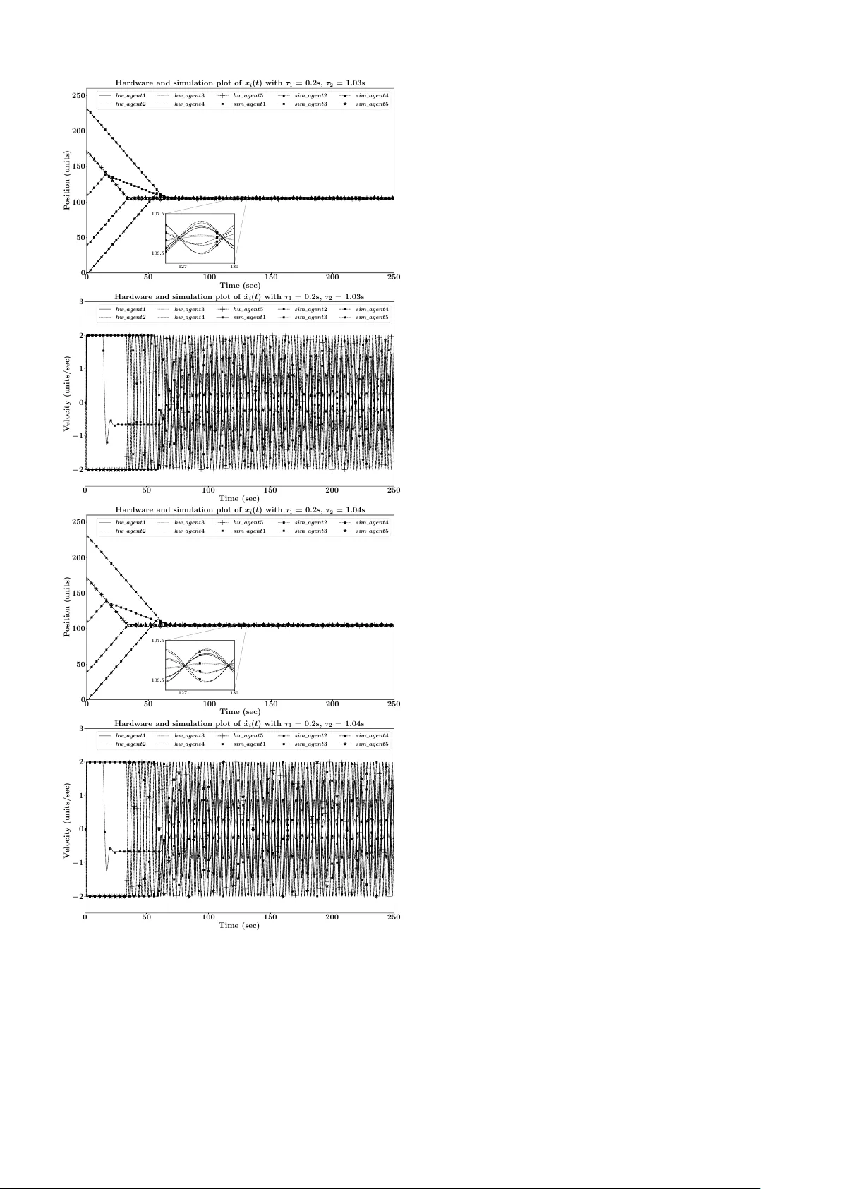
IET Research Journals Brief Paper: This paper is a postprint of a paper submitted to and accepted for pub lication in IET Control Theor y & Applications and is subject to Institution of Engineering and T echnology Cop yright. The copy of record is a v ailable at the IET Digital Library Consensus of second or der m ulti-a gents with actuator saturation and asynchr onous time-dela ys ISSN 1751-8644 doi: 0000000000 www .ietdl.org V enkata Kar teek Y anumula 1 Indrani Kar 1 Somanath Majhi 1 1 Dept. of EEE, IIT Guwahati-781039, India. * E-mail: yanum ula@iitg.er net.in Abstract: This ar ticle presents the consensus of a saturated second order multi-agent system with non-switching dynamics that can be represented by a directed graph. The system is affected by data processing (input dela y) and communication time-delays that are assumed to be asynchronous. The agents have saturation nonlinear ities, each of them is appro ximated into separate linear and nonlinear elements. Nonlinear elements are represented by describing functions. Descr ibing functions and stability of linear elements are used to estimate the existence of limit cycles in the system with multiple control laws . Stability analysis of the linear element is performed using Ly apunov-Krasovskii functions and frequency domain analysis. A comparison of pros and cons of both the analyses with respect to time-dela y ranges, applicability and computation complexity is presented. Simulation and corresponding hardware implementation results are demonstrated to suppor t theoretical results. 1 Introduction In the recent past, multi-agent systems have attracted a lot of atten- tion due to their wide range of application in robotics, unmanned air and underwater vehicles, automated traffic signal control, wireless sensor networks, etc.. One of the most important problems in coor- dinated control is consensus of a multi-agent system, which deals with algorithms required for the conv ergence of agents [1, 2]. After the initial study by V icsek et al. [3] on self-ordered motions in bio- logically motiv ated particles, Jadbabaie et al. [1] ga ve the theoretical explanation. Olfati-Saber et al. [2] provided mathematical analysis of consensus behaviour in linear first order agents with time-delay using graph theory concepts. Multi-agent consensus problems with higher order agents, switching topologies, time-delays, nonlineari- ties etc., started recei ving more attention [4, 5] after the initial results giv en by authors in [1, 2]. Howe ver , the majority of control laws are designed to solve con- sensus problems in linear multi-agent systems [1, 2, 6–12]. For linear systems, it has been sho wn that eigen values of graph laplacian play an important role in estimating whether the network of agents con verge. Since nonlinearities are unavoidable in most of the prac- tical applications, nonlinear agents and the corresponding control laws are being considered recently [13–15]. Mobile agents gener- ally have limited capability due to factors like actuator saturation, moment of inertia, maximum limit on velocity , etc.. Actuator satura- tion is frequently encountered due to limitations in hardware. Some of the researchers focused on consensus in multi-agent systems with saturation in first order [16] and second order agents [17–22]. Apart from eigenv alues of graph laplacian, time-delays play ma- jor role in stability of multi-agent network. In practical applications, time-delays are inevitable and are classified into two categories; communication and input time-delays. The amount of time taken by agents to communicate is defined as communication time-delay and the amount of time taken by agents to process the information receiv ed from other agents is called input time-delay . Olfati-Saber et al. [2] started the analysis of time-delay effects on multi-agent systems and gav e an upper bound for first order agents considering constant uniform communication and input time-delays. Later on it was extended to systems with first order agents and uniform time- varying delay[6] multiple delays [9, 23], second order agents with constant time-delays [8, 24] and system with second order agents with non-uniform delay [11]. The majority of research is confined to linear agents with time- delays and recently nonlinear agents with time-delays are receiving attention [14, 22]. Furthermore, nonlinearities are common in mobile agents and actuator saturation is the most frequent hard nonlinearity affecting them. For example, the acceleration of an agent is constant ov er certain range and cannot be maintained after the agent attains its maximum velocity . Recently , saturation nonlinearity is receiving considerable attention. Li et al. [16] considered a first order system with saturation and without time-delays. For second order agents with saturation and without time-delay , a differential gain feedback control is used by authors in [17, 18]. Adapti ve control laws with an observer are used by Chu et al. [19] and nonlinear agents are consid- ered by Cui et al. [21]. The effects of synchronous time-delays are taken into consideration by Y ou et al. [22] for a network of second order saturated agents. It is e vident from the literature that, there is very little focus on consensus of second order saturated multi-agent system with asyn- chronous communication and input time-delays. In this contrib ution, a multi-agent system is considered with asynchronous time-delays and hard saturation nonlinearities. The objective of the article is to extend the results of Liu et al. [14] for velocity saturated nonlin- ear multi-agent system with time-delays using a different approach. Describing function analysis [25] is used to break agents into ap- proximate linear and nonlinear elements, with the nonlinear element represented by an appropriate describing function. The difference among position states and velocity states of agents is defined as error dynamics. The system achiev es consensus when the error dynamics are asymptotically stable. Here, the existence of limit cycles in the multi-agent system is estimated with the help of describing functions and stability of linear element. L yapunov-Krasovskii functions and frequency domain analysis are used to prove the stability of linear element and further estimate the stability of limit cycles. Consensus is achiev ed when there are no limit cycles. Some necessary and suf- ficient conditions for consensus in terms of linear matrix inequalities and explicit expressions are derived. The major contributions of the paper can be summarised as, 1. Deriving v arious conditions for four consensus control laws with asynchronous time-delays; 2. Describ- ing function analysis is used to estimate the limit cycle behaviour of the system; 3. Stability analysis of the linear element using L ya- punov-Kraso vskii and frequency domain approaches is performed; 4. A comparison of pros and cons of both the stability analyses is presented; 5. Simulations and further validation of results on a IET Research Journals, pp. 1–10 c  The Institution of Engineering and T echnology 2015 1 four-agent and a fiv e-agent networks are demonstrated to support theoretical analysis. The rest of the paper is organised as follows, Section 2 explains graph theory preliminaries. Section 3 elaborates the system model with four control laws given in Eqns. (5) to (8). Stability analysis is performed using L yapunov-Krasovskii functions for control laws in Eqns. (5) to (8), using the Nyquist stability criterion for control laws in Eqns. (5) and (6). Furthermore, simulation and implementa- tion of the control laws on two networks are explained. Depiction of results and comparison of the two stability procedures are performed in Section 4. 2 Preliminaries 2.1 Graph theor y Graph theory is widely used to study multi-agent systems. A net- work of agents and the underlying communication topology can be represented by a graph G = ( V , E , A ) . If the communication among agents could be unidirectional, a directed graph is used to describe the multi-agent network. The v ertex set V = { v 1 , v 2 , ...., v n } where vertices are analogous to agents and an edge set E = { ( i, j ) : i, j ∈ V } where edges are analogous to the branches of directed network with ( i, j ) representing information flowing from j th verte x to i th . Edge set has distinct ordered pairs of v ertices which depict existence and direction of information flow among the vertices. An adjacency matrix A = ( a ij ) n × n also represents communication topology with a ij = 1 if ( i, j ) ∈ E and a ij = 0 otherwise. A weighted adjacency matrix will have entries other than zero and unity weights depend- ing on the assumptions of cost of communication. If there exists at least one vertex which has a directed path to all the other vertices, the graph is said to form a spanning tree and if all the vertices hav e directed paths to all the other agents, it is called strongly connected. A spanning tree condition is a necessary condition for consensus but not suf ficient when time-delays and higher order systems are in- volv ed [4, 5]. The sum of weights of inward branches at a vertex is called in-degree d in ( v i ) and the weight sum of outward branches is called out-degree of the v ertex d out ( v i ) . 2.2 Notations The following notations are used throughout the paper , R n repre- sents an n -dimensional Euclidean space. R m × n represent a space of m × n matrices. Position and velocity of n agents are rep- resented by x = [ x 1 x 2 ... x n ] T and ˙ x = v respecti vely . X = [ X 1 X 2 ... X n X n +1 ... X 2 n ] T represent the states of a multi-agent system with [ X 1 X 2 ... X n ] T = x and [ X n +1 ... X 2 n ] T = ˙ x . I n and I 2 n represent identity matrices of sizes n × n and 2 n × 2 n re- spectiv ely . 1 n is a vector ones of size 1 × n . For { A, B } ∈ R n × n , if A < B , then A − B is positi ve semidefinite; if A  B , then A − B is positiv e definite. D represents a matrix with diagonal elements as row-sum of adjacenc y matrix A and rest of the elements as zero. A matrix ˜ A is defined with elements ˜ a ij = a ij P n j =1 a ij and [ ˜ λ 1 , ˜ λ 2 , ..., ˜ λ n ] are the eigen values of matrix ˜ A . 3 System model and analysis Consider a multi-agent network of homogeneous second order agents with i th agent dynamics giv en in Eqn. (1), ˙ x i ( t ) = sat (ˆ v i ( t )) ˙ ˆ v i ( t ) = u i ( t ) (1) For mobile agents, the position of an agent is represented by x i ( t ) and the velocity by ˙ x i ( t ) . V arious control protocols used in the anal- ysis are given in Eqns. (5) to (8). It is assumed that ∀ t ∈ ( −∞ , 0] , x i ( t ) = x (0) and ˆ v i ( t ) = 0 . Saturation nonlinearity used in the system is defined in Eqn. (2) with ± ∆ as bounds. sat ( α ) =      − ∆ , if α ≤ − ∆ α, if − ∆ < α < ∆ ∆ , if α ≥ ∆ (2) The i th agent dynamics are depicted using a block diagram giv en Z ∆ − ∆ Z Communication & process ˆ v i v i ( a j i )( x i , v i ) ( a ij )( x j , v j ) x i u i Fig. 1 : Block diagram of i th agent. in Fig. 1. Using the concepts of describing function to estimate limit cycles [25], the system can be approximately transformed as shown in Fig. 2. Since a single-valued nonlinearity is considered, its ap- proximate describing function for the saturation is given in Eqn. (3) [25], N ( A ) = 2 π " arcsin  ∆ A  + ∆ A r 1 − ∆ 2 A 2 # (3) where, the limit cycles’ amplitude is represented by A . The describing function is real valued and − 1 / N ( A ) ∈ [ − 1 , ∞ ) , it can be estimated that the limit cycles are stable when the transfer function of linear element in Fig. 2 encircles ( − 1 , 0) in a complex plane. In other words, limit c ycles are exhibited when the linear ele- ment is unstable in the multi-agent system. Stability analysis of the linear element is performed using L yapunov-Krasovskii approach in Section 3.1 and Nyquist stability approach giv en in Section 3.2. Nonlinear element Communication & process Linear element ( x i , v i ) u i Fig. 2 : Rearranged block diagram of i th agent. The approximate linear element given in Fig. 2 is represented by Eqn. (4), ˙ x i ( t ) = v i ( t ) ˙ v i ( t ) = u i ( t ) (4) V arious control laws considered from the literature for analysis are giv en in Eqns. (5) to (8), u i 1 ( t ) = − v i ( t − τ 1 ) + 1 P n j =1 a ij n X j =1  a ij  x j ( t − τ 2 ) − x i ( t − τ 1 )   (5) u i 2 = 1 P n j =1 a ij n X j =1  a ij  v j ( t − τ 2 ) − v i ( t − τ 1 )  + a ij  x j ( t − τ 2 ) − x i ( t − τ 1 )   (6) u i 3 ( t ) = − v i ( t − τ 1 ) + n X j =1  a ij  x j ( t − τ 2 ) − x i ( t − τ 1 )   (7) IET Research Journals, pp. 1–10 2 c  The Institution of Engineering and T echnology 2015 u i 4 = n X j =1  a ij  v j ( t − τ 2 ) − v i ( t − τ 1 )  + a ij  x j ( t − τ 2 ) − x i ( t − τ 1 )   (8) where τ 1 and τ 2 represent input and communication time-delays re- spectiv ely . W ith an y of the control la ws in Eqns. (5) to (8), consensus is said to be reached if ( x i ( t ) − x j ( t )) → 0 and ( ˙ x i ( t ) − ˙ x j ( t )) → 0 ∀{ i, j } ∈ [1 , n ] . Control laws in Eqns. (5) and (6) generate lesser magnitude of control input u i which result in slightly larger con ver- gence time compared to the ones in Eqns. (7) and (8). The a veraging in control laws gi ven by Eqns. (5) and (6) have better time-delay tol- erance due to smaller Fiedler eigen value compared to control laws in Eqns. (7) and (8) at the expense of con vergence time. W ith control laws in Eqns. (5) and (7), the state ˙ x i ( t ) → 0 when the consensus is achie ved since they do not consider difference in velocity . State ˙ x i ( t ) → 0 is not guaranteed with control laws in Eqns. (6) and (8). 3.1 L yapuno v-Krasovskii approach Consider the linear element represented in Eqns. (4) to (8), which can be represented as giv en in Eqn. (9). ˙ X ( t ) = A 0 X ( t ) + A 1 X ( t − τ 1 ) + A 2 X ( t − τ 2 ) (9) Where A 0 , A 1 and A 2 are as giv en in Eqns. (10) to (13). For u i 1 giv en in Eqn. (5), A 0 =  0 n × n I n 0 n × n 0 n × n  ; A 1 =  0 n × n 0 n × n − I n − I n  ; A 2 =  0 n × n 0 n × n e A 0 n × n  (10) For u i 2 giv en in Eqn. (6), A 0 =  0 n × n I n 0 n × n 0 n × n  ; A 1 =  0 n × n 0 n × n − I n − I n  ; A 2 =  0 n × n 0 n × n e A e A  (11) For u i 3 giv en in Eqn. (7), A 0 =  0 n × n I n 0 n × n 0 n × n  ; A 1 =  0 n × n 0 n × n − D − I n  ; A 2 =  0 n × n 0 n × n A 0 n × n  (12) For u i 4 giv en in Eqn. (8), A 0 =  0 n × n I n 0 n × n 0 n × n  ; A 1 =  0 n × n 0 n × n − D − D  ; A 2 =  0 n × n 0 n × n A A  (13) Some definitions and lemmas analogous to the ones in [26] are given below , Definition 1. Balanced graph : A graph is said to be balanced if in- degree equals to out-degree for all vertices in the graph, d in ( v i ) = d out ( v i ) , ∀ i ∈ [1 , n ] . Definition 2. k -r e gular graph : It is a balanced graph with all the vertices having in-degree and out-degree equal to k , d in ( v i ) = d out ( v i ) = k , ∀ i ∈ [1 , n ] Control laws given in Eqns. (5) and (6) make the multi-agent system behav e like a system connected by 1-regular graph. Lemma 1. Consider Φ 01 = 1 n  1 n × n 0 n × n 0 n × n 1 n × n  and E = I 2 n − Φ 01 , then the following statements hold true: 1. A multi-agent system with k -re gular graph communication topol- ogy and with inputs in Eqns. (5) to (8) produces balanced matrices E ( A 0 + A 1 + A 2 ) , E A 0 , E A 1 , E A 2 and E ( A 1 + A 2 ) with maximum rank 2 n − 2 and eigen values 0 of multiplicity atleast two. 2. A multi-agent system with a spanning tr ee in communication topol- ogy and with inputs in Eqns. (5) and (6) produces balanced matrices E ( A 0 + A 1 + A 2 ) , E A 0 , E A 1 , E A 2 and E ( A 1 + A 2 ) with maximum rank 2 n − 2 and eigen values 0 of multiplicity atleast two. Definition 3. Balanced matrix : A square matrix M ∈ R n × n is said to be balanced iff M 1 T n = 0 and 1 n M = 0 . Lemma 2. Consider Φ 01 = 1 n  1 n × n 0 n × n 0 n × n 1 n × n  and E = I 2 n − Φ 01 , then the following statements hold true for k -re gular graph with inputs in Eqns. (5) to (8) and for spanning tree graph with inputs in Eqns. (5) and (6) : 1. E ( A 0 + A 1 + A 2 ) is a balanced matrix with rank 2 n − 2 and eigen values 0 of multiplicity 2 . 2. Matrices E A 0 , E A 1 , E A 2 and E ( A 1 + A 2 ) ar e all balanced with eigen values 0 of multiplicity atleast 2 . 3. Ther e is a matrix U , an ortho gonal matrix of eigen vectors of E which satisfies, U T E U =  e E (2 n − 2) × 2 0 (2 n − 2) × 2 0 2 × (2 n − 2) 0 2 × 2  4. Let E A 0 = F 0 , E A 1 = F 1 and E A 2 = F 2 . E , F 0 , F 1 and F 2 have maximum rank 2 n − 2 and with zer o r ow sums, then, U T F i U =  e F i (2 n − 2) × (2 n − 2) 0 (2 n − 2) × 2 0 2 × (2 n − 2) 0 2 × 2  , i ∈ [0 , 2] . 5. Also, for cases of τ 1 = τ 2 > 0 and τ 1 = τ 2 = 0 , U T E ( A 1 + A 2 ) U =  ( e F 1 + e F 2 ) (2 n − 2) × (2 n − 2) 0 (2 n − 2) × 2 0 2 × (2 n − 2) 0 2 × 2  U T E ( A 0 + A 1 + A 2 ) U =  ( e F 0 + e F 1 + e F 2 ) 0 (2 n − 2) × 2 0 2 × (2 n − 2) 0 2 × 2  Let the difference in position and velocity among the agents be assumed as error Ψ , each element of Ψ is giv en by Eqn. (14) Ψ i =          1 n n P j =1  X i − X j  ∀ i ∈ [1 , n ] 1 n 2 n P j = n +1  X i − X j  ∀ i ∈ [ n + 1 , 2 n ] (14) From the assumption in Lemma 1, Ψ = E X (15) Lemma 3. When error Ψ → 0 , then x i → x j and v i → v j . Con- versely when x i → x j and v i → v j , then Ψ → 0 . Proof . Consider a matrices, γ n × n =        1 − 1 0 ... 0 0 1 − 1 ... 0 ... ... ... ... ... ... ... ... ... ... 0 ... 0 1 − 1 − 1 0 ... 0 1        (16) Γ 2 n × 2 n =  γ n × n 0 n × n 0 n × n γ n × n  (17) IET Research Journals, pp. 1–10 c  The Institution of Engineering and T echnology 2015 3 Multiplying with Γ on both sides of Eqn. (15),               Ψ 1 − Ψ 2 Ψ 2 − Ψ 3 . . Ψ n − Ψ 1 Ψ n +1 − Ψ n +2 Ψ n +2 − Ψ n +3 . . Ψ 2 n − Ψ n +1               =               X 1 − X 2 X 2 − X 3 . . X n − X 1 X n +1 − X n +2 X n +2 − X n +3 . . X 2 n − X n +1               (18) When Ψ → 0 , left side of Eqn. (18) becomes 0 2 n × 1 . Which implies, X i → X j , ∀{ i, j } ∈ [1 , n ] and X i → X j , ∀{ i, j } ∈ [ n + 1 , 2 n ] . From Eqn. (14), when x i → x j and v i → v j , then Ψ → 0 .  A control input is said to have solved the consensus problem in a globally asymptotic manner when x i → x j and v i → v j , in other words, Ψ → 0 . Stability of linear element with the control inputs estimates the existence of limit c ycles in the system. Theorem 1. Consider the linear element in Eqn. (4) with time- delays ( τ 1 , τ 2 ) ≥ 0 , τ 1 ≤ τ 2 . The contr ol inputs for a k -re gular graph given in Eqns. (5) to (8) and the contr ol inputs for a span- ning tr ee graph given in Eqns. (5) and (6) globally asymptotically solve consensus problem, if there exist matrices e P > 0 , e Q 1 > 0 , e Q 2 > 0 , e Z i > 0 , ∀ i ∈ [1 , 3] , e F i fr om Lemma 2 ∀ i ∈ [1 , 3] and arbi- trary matrices { e H ij , e H T ij , e I ij , e I T ij , e J ij , e J T ij } ∀ i ∈ [1 , 3] ∀ j ∈ [1 , 4] of size (2 n − 2) × (2 n − 2) suc h that,   e G 11 e G 12 e G 13 e G T 12 e G 22 e G 23 e G T 13 e G T 23 e G 33   ≺ 0 (19)     e H 11 e H 12 e H 13 e H 14 e H T 12 e H 22 e H 23 e H 24 e H T 13 e H T 23 e H 33 e H 34 e H T 14 e H T 24 e H T 34 e Z 1     < 0 (20)     e I 11 e I 12 e I 13 e I 14 e I T 12 e I 22 e I 23 e I 24 e I T 13 e I T 23 e I 33 e I 34 e I T 14 e I T 24 e I T 34 e Z 2     < 0 (21)     e J 11 e J 12 e J 13 e J 14 e J T 12 e J 22 e J 23 e J 24 e J T 13 e J T 23 e J 33 e J 34 e J T 14 e J T 24 e J T 34 e Z 3     < 0 (22) wher e, e G 11 = e F T 0 e P e E + e E T e P e F 0 + e E T e Q 1 e E + e E T e Q 2 e E + e F T 0 e Ξ e F 0 + τ 1 e E T e H 11 e E + e E T e H 14 e E + e E T e H T 14 e E + τ 2 e E T e I 11 e E + e E T e I 14 e E + e E T e I T 14 e E + ( τ 2 − τ 1 ) e E T e J 11 e E (23) e G 12 = e E T P e F 1 + e F T 0 e Ξ e F 1 + τ 1 e E T e H 12 e E − e E T e H 14 e E + e E T e H T 24 e E + τ 2 e E T e I 12 e E + e E T e I T 24 e E + ( τ 2 − τ 1 ) e E T e J 12 e E + e E T e J 14 e E (24) e G 13 = e E T e P e F 2 + e F T 0 e Ξ e F 2 + τ 1 e E T e H 13 e E + e E T e H T 34 e E + e E T e I T 34 e E + τ 2 e E T e I 13 e E − e E T e I 14 e E + ( τ 2 − τ 1 ) e E T e J 13 e E − e E T e J 14 e E (25) e G 22 = − e E T e Q 1 e E + e F T 1 e Ξ e F 1 + τ 1 e E T e H 22 e E − e E T e H 24 e E − e E T e H T 24 e E + τ 2 e E T e I 22 e E + ( τ 2 − τ 1 ) e E T e J 22 e E + e E T e J 24 e E + e E T e J T 24 e E (26) e G 23 = e F T 1 e Ξ e F 2 + τ 1 e E T e H 23 e E − e E T e H T 34 e E + τ 2 e E T e I 23 e E − e E T e I 24 e E + ( τ 2 − τ 1 ) e E T e J 23 e E − e E T e J 24 e E + e E T e J T 34 e E (27) e G 33 = − e E T e Q 2 e E + e F T 2 e Ξ e F 2 + τ 1 e E T e H 33 e E − e E T e I 34 e E − e E T e I T 34 e E + τ 2 e E T e I 33 e E + ( τ 2 − τ 1 ) e E T e J 33 e E − e E T e J 34 e E − e E T e J T 34 e E (28) e Ξ = τ 1 e Z 1 + τ 2 e Z 2 + ( τ 2 − τ 1 ) e Z 3 (29) Proof . Let P , Q 1 , Q 2 , Z i i ∈ [1 , 3] be balanced positive semi- definite matrices of rank 2 n − 2 and Ψ = E X using E from Lemma 1. The L yapunov-Krasovskii functional is assumed as, V ( Ψ ( t )) = Ψ T ( t ) P Ψ ( t ) + Z t t − τ 1 Ψ T ( s ) Q 1 Ψ ( s ) ds + Z t t − τ 2 Ψ T ( s ) Q 2 Ψ ( s ) ds + Z 0 − τ 1 Z t t + θ ˙ Ψ T ( s ) Z 1 ˙ Ψ ( s ) dsdθ + Z 0 − τ 2 Z t t + θ ˙ Ψ T ( s ) Z 2 ˙ Ψ ( s ) dsdθ + Z − τ 1 − τ 2 Z t t + θ ˙ Ψ T ( s ) Z 3 ˙ Ψ ( s ) dsdθ (30) ˙ V ( Ψ ( t )) = ˙ Ψ T ( t ) P Ψ ( t ) + Ψ T ( t ) P ˙ Ψ ( t ) + Ψ T ( t ) Q 1 Ψ ( t ) + Ψ T ( t ) Q 2 Ψ ( t ) − Ψ T ( t − τ 1 ) Q 1 Ψ ( t − τ 1 ) − Ψ T ( t − τ 2 ) Q 2 Ψ ( t − τ 2 ) + τ 1 ˙ Ψ T ( t ) Z 1 ˙ Ψ ( t ) + τ 2 ˙ Ψ T ( t ) Z 2 ˙ Ψ ( t ) + ( τ 2 − τ 1 ) ˙ Ψ T ( t ) Z 3 ˙ Ψ ( t ) − Z 0 − τ 1 ˙ Ψ T ( t + θ ) Z 1 ˙ Ψ ( t + θ ) dθ − Z 0 − τ 2 ˙ Ψ T ( t + θ ) Z 2 ˙ Ψ ( t + θ ) dθ − Z − τ 1 − τ 2 ˙ Ψ T ( t + θ ) Z 3 ˙ Ψ ( t + θ ) dθ (31) Let, c X = h X ( t ) T X ( t − τ 1 ) T X ( t − τ 2 ) T i (32) then, ˙ Ψ = E ˙ X = E  A 0 A 1 A 2  c X T (33) ˙ Ψ T ( t ) P Ψ ( t ) = c X  A 0 A 1 A 2  T E T P E X ( t ) (34) Ψ T ( t ) P ˙ Ψ ( t ) = X ( t ) T E T P E  A 0 A 1 A 2  c X T (35) Ψ T ( t ) Q 1 Ψ ( t ) = X ( t ) T E T Q 1 E X ( t ) (36) IET Research Journals, pp. 1–10 4 c  The Institution of Engineering and T echnology 2015 Ψ T ( t ) Q 2 Ψ ( t ) = X ( t ) T E T Q 2 E X ( t ) (37) Ψ T ( t − τ 1 ) Q 1 Ψ ( t − τ 1 ) = X ( t − τ 1 ) T E T Q 1 E X ( t − τ 1 ) (38) Ψ T ( t − τ 2 ) Q 2 Ψ ( t − τ 2 ) = X ( t − τ 2 ) T E T Q 2 E X ( t − τ 2 ) (39) For i = { 1 , 2 , 3 } , ˙ Ψ T ( t ) Z i ˙ Ψ ( t ) = c X  A 0 A 1 A 2  T E T Z i E  A 0 A 1 A 2  c X T (40) Consider a set of matrices,     H 11 H 12 H 13 H 14 H T 12 H 22 H 23 H 24 H T 13 H T 23 H 33 H 34 H T 14 H T 24 H T 34 Z 1     < 0 (41)     I 11 I 12 I 13 I 14 I T 12 I 22 I 23 I 24 I T 13 I T 23 I 33 I 34 I T 14 I T 24 I T 34 Z 2     < 0 (42)     J 11 J 12 J 13 J 14 J T 12 J 22 J 23 J 24 J T 13 J T 23 J 33 J 34 J T 14 J T 24 J T 34 Z 3     < 0 (43) Where H ij , I ij , J ij ∀ i ∈ [1 , 3] ∀ j ∈ [1 , 4] are some arbitrary matri- ces to be found by an LMI solver with size 2 n × 2 n . Let, b Ψ ˙ θ = h Ψ ( t ) T Ψ ( t − τ 1 ) T Ψ ( t − τ 2 ) T ˙ Ψ ( t + θ ) T i (44) then, Z 0 − τ 1 b Ψ ˙ θ     H 11 H 12 H 13 H 14 H T 12 H 22 H 23 H 24 H T 13 H T 23 H 33 H 34 H T 14 H T 24 H T 34 Z 1     b Ψ T ˙ θ dθ ≥ 0 (45) Z 0 − τ 2 b Ψ ˙ θ     I 11 I 12 I 13 I 14 I T 12 I 22 I 23 I 24 I T 13 I T 23 I 33 I 34 I T 14 I T 24 I T 34 Z 2     b Ψ T ˙ θ dθ ≥ 0 (46) Z − τ 1 − τ 2 b Ψ ˙ θ     J 11 J 12 J 13 J 14 J T 12 J 22 J 23 J 24 J T 13 J T 23 J 33 J 34 J T 14 J T 24 J T 34 Z 3     b Ψ T ˙ θ dθ ≥ 0 (47) The matrices in Ineqs. (41) to (43) are chosen to satisfy expression in Ineqs. (45) to (47), which further simplify ˙ V in Eqn. (31). Parts of Eqn. (31) consisting integrals with multiplication two variable in terms of θ are eliminated when added with Ineqs. (45) to (47), since ˙ V + { positiv e semidef inite } < 0 implies ˙ V < 0 . Substi- tuting Eqns. (32) to (40) in Eqn. (31), adding Ineqs. (45) to (47) and further solving leftov er integrals, Ineq. (48) is obtained. ˙ V ≤ c X   G 11 G 12 G 13 G T 12 G 22 G 23 G T 13 G T 23 G 33   c X T (48) where, G 11 = A T 0 E T P E + E T P E A 0 + E T Q 1 E + E T Q 2 E + (49) A T 0 E T Ξ E A 0 + τ 1 E T H 11 E + E T H 14 E + E T H T 14 E + τ 2 E T I 11 E + E T I 14 E + E T I T 14 E + ( τ 2 − τ 1 ) E T J 11 E G 12 = E T P E A 1 + A T 0 E T Ξ E A 1 + τ 1 E T H 12 E − E T H 14 E + E T H T 24 E + τ 2 E T I 12 E + E T I T 24 E + ( τ 2 − τ 1 ) E T J 12 E + E T J 14 E (50) G 13 = E T P E A 2 + A T 0 E T Ξ E A 2 + τ 1 E T H 13 E + E T H T 34 E + τ 2 E T I 13 E + E T I T 34 E − E T I 14 E + ( τ 2 − τ 1 ) E T J 13 E − E T J 14 E (51) G 22 = − E T Q 1 E + A T 1 E T Ξ E A 1 + τ 1 E T H 22 E − E T H 24 E − E T H T 24 E + τ 2 E T I 22 E + ( τ 2 − τ 1 ) E T J 22 E + E T J 24 E + E T J T 24 E (52) G 23 = A T 1 E T Ξ E A 2 + τ 1 E T H 23 E − E T H T 34 E + τ 2 E T I 23 E − E T I 24 E + ( τ 2 − τ 1 ) E T J 23 E − E T J 24 E + E T J T 34 E (53) G 33 = − E T Q 2 E + A T 2 E T Ξ E A 2 + τ 1 E T H 33 E − E T I 34 E − E T I T 34 E + τ 2 E T I 33 E + ( τ 2 − τ 1 ) E T J 33 E − E T J 34 E − E T J T 34 E (54) Ξ = τ 1 Z 1 + τ 2 Z 2 + ( τ 2 − τ 1 ) Z 3 (55) The matrices P , Q 1 , Q 2 , Z i , H ij , H T ij , I ij , I T ij , J ij , J T ij and F i from Lemma 2 ∀ i ∈ [1 , 3] , ∀ j ∈ [1 , 4] will generate corresponding e P , e Q 1 , e Q 2 , e Z i , e H ij , e H T ij , e I ij , e I T ij , e J ij , e J T ij and e F i ∀ i ∈ [1 , 3] , ∀ j ∈ [1 , 4] of size (2 n − 2) × (2 n − 2) when multiplied with eigenv ec- tor matrices U T , U at appropriate positions. The corresponding G ij is as giv en in Eqn. (56). G ij = U  e G ij (2 n − 2) × (2 n − 2) 0 (2 n − 2) × 2 0 2 × (2 n − 2) 0 2 × 2  U T { i, j } ∈ [1 , 3]; e G j i = e G T j i ∀ i 6 = j (56) W ith above set of reduced order matrices, the LMIs gi ven in Eqns. (19) to (22) can be obtained.  Feasibility of LMIS in Eqns. (19) to (22) determine the consensus reachability of the multi-agent system af fected by time-delays. The y can be solved by using solvers like SeDuMi [27], Matlab LMI Lab solver etc.. 3.2 Nyquist stability approach Stability analysis of the linear element for different control inputs is performed using frequency domain analysis and Nyquist stability criterion which is discussed in Sections 3.2.1 and 3.2.2. 3.2.1 First control law: Consider a control input u i 1 with input delay τ 1 and communication delay τ 2 as gi ven in Eqn. (5) assuming τ 1 ≤ τ 2 . Theorem 2. The system r epr esented by Eqns. (4) and (5) is stable if and only if, | ˜ λ k | q ω 4 − 2 ω 3 sin ( ωτ 1 ) + ω 2 (1 − 2 cos ( ω τ 1 )) + 1 < 1 (57) IET Research Journals, pp. 1–10 c  The Institution of Engineering and T echnology 2015 5 wher e ω satisfies − π = − ω τ 2 + arg  − ˜ λ k  − arctan  ω cos ( ω τ 1 ) − sin ( ω τ 1 ) − ω 2 + cos ( ω τ 1 ) + ω sin ( ω τ 1 )  (58) Proof . The system in Eqns. (4) and (5) can also be represented as, ¨ x i ( t ) = − ˙ x i ( t − τ 1 ) + 1 P n j =1 a ij n X j =1 a ij  x j ( t − τ 2 ) − x i ( t − τ 1 )  (59) Con verting it into s domain will give the characteristic expression as,    s 2 I + ( s + 1) I e − sτ 1 − ˜ A e − sτ 2    = n Y k =1  s 2 I + ( s + 1) I e − sτ 1 − ˜ λ k e − sτ 2  (60) Consider ∀ ˜ λ k 6 = 0 , G k ( s ) = − ˜ λ k e − sτ 2 s 2 + ( s + 1) e − sτ 1 (61) Magnitude expression of Eqn. (61) is gi ven by ,   G k ( j ω )   = | ˜ λ k | p ω 4 − 2 ω 3 sin ( ωτ 1 ) + ω 2 (1 − 2 cos ( ω τ 1 )) + 1 (62) Phase expression of Eqn. (61) is gi ven by , G k ( j ω ) = − ω τ 2 + arg  − ˜ λ k  − arctan  ω cos ( ω τ 1 ) − sin ( ω τ 1 ) − ω 2 + cos ( ω τ 1 ) + ω sin ( ω τ 1 )  (63) Let us assume at ω = ω , the Nyquist plot intersects with negati ve real axis. The phase at ω = ω is − π , − π = − ω τ 2 + arg  − ˜ λ k  − arctan  ω cos ( ω τ 1 ) − sin ( ω τ 1 ) − ω 2 + cos ( ω τ 1 ) + ω sin ( ω τ 1 )  (64) By applying Nyquist stability criterion, magnitude given in Eqn. (62) should satisfy the condition as giv en in Ineq. (65). | ˜ λ k | q ω 4 − 2 ω 3 sin ( ωτ 1 ) + ω 2 (1 − 2 cos ( ω τ 1 )) + 1 < 1 (65)  3.2.2 Second control law: Consider control input u i 2 giv en in Eqn. (6), where, Theorem 3. The system repr esented in Eqns. (4) and (6) is stable if and only if, | ˜ λ k | p 1 + ω 2 q ω 4 − 2 ω 3 sin ( ωτ 1 ) + ω 2 (1 − 2 cos ( ω τ 1 )) + 1 < 1 (66) wher e ω satisfies, − π = − ω τ 2 + arg  − ˜ λ k  + arctan ( ω ) − arctan  ω cos ( ω τ 1 ) − sin ( ω τ 1 ) − ω 2 + cos ( ω τ 1 ) + ω sin ( ω τ 1 )  (67) Proof . The proof follows a similar procedure as gi ven in Theorem 2  4 Simulation and Implementation Results The communication topologies considered for simulation and im- plementation are depicted in Figs. 3a and 3b. The graph in Fig. 3a is undirected, strongly connected and 2-regular balanced with each node receiving states’ information from two neighbours and send- ing states’ information to the same neighbours. The graph in Fig. 3b is directed, has a spanning tree and unbalanced. Using the results obtained in Theorems 1 to 3, limits on communication time-delay for giv en input-delays are calculated for both the topologies. The feasibility of LMIs gi ven in Theorem 1 is solved using SeDuMi [27] solver for Matlab/Octa ve. The expressions in Theorems 2 and 3 ha ve three unknowns ( ω , τ 1 , τ 2 ) , a unique solution can be obtained if it is assumed that τ 1 = τ 2 or else, stable range of τ 2 for a giv en τ 1 hav e to be found. Dominant pole for both the topologies in Figs. 3a and 3b is − 1 , Nyquist plot used in one of the cases with λ = − 1 and assumption τ 1 = 0 . 4 is shown in Fig. 4. It can be observed that the system is stable if τ 2 < 0 . 48 (Fig. 4). The time-delay tolerances are tested with simulations and on a hardw are setup (Fig. 5). The results obtained using L yapunov-Krasovskii and Nyquist approaches from Theorems 1 to 3 are tabulated in T ables 1 and 2, corresponding plots of τ 1 vs τ 2 depicting stable regions are gi ven in Figs. 6a and 6b. 1 2 3 4 (a) Four agents. 1 2 3 4 5 (b) Fiv e agents. Fig. 3 : Graphs of communication topologies. − 1.25 − 1.00 − 0.75 − 0.50 − 0.25 0.00 0.25 0.50 Real − 1.50 − 1.25 − 1.00 − 0.75 − 0.50 − 0.25 0.00 0.25 0.50 Imaginary Nyquist plot for λ = -1 with τ 1 = 0.4 τ 2 =0.478 τ 2 =0.479 τ 2 =0.48 − 1.01 − 1.00 − 0.99 0.01 0.00 − 0.01 Fig. 4 : Nyquist plot with u i 1 in Eqn. (5) for different time delays. From the results in T ables 1 and 2 and Figs. 6a and 6b, it can be deduced that the L yapunov-Krasovskii approach is conserv ativ e compared to Nyquist approach with respect to time-delay . Conser- vati veness of L yapunov-Krasovskii approach is more evident for topology in Fig. 3b with control la w in Eqn. (6). Multi-agent systems connected by topologies in Figs. 3a and 3b reach consensus with full range of time-delay giv en by Nyquist approach for control laws in Eqns. (5) and (6). Nyquist approach in Section 3.2 is not applicable IET Research Journals, pp. 1–10 6 c  The Institution of Engineering and T echnology 2015 Fig. 5 : Hardware setup connected by LAN. to control laws giv en in Eqns. (7) and (8). Solving LMIs is com- putationally more intensiv e compared to solving of equations from Theorems 2 and 3. Moreover , the increase in computational time of solving LMIs is exponentially as the number of nodes are increased and the increase with Nyquist approach is linear . 0 . 00 0 . 05 0 . 10 0 . 15 0 . 20 0 . 25 0 . 30 0 . 35 0 . 40 0 . 45 0 . 50 0 . 55 Input dela y τ 1 (sec) 0 . 0 0 . 1 0 . 2 0 . 3 0 . 4 0 . 5 0 . 6 0 . 7 0 . 8 0 . 9 1 . 0 1 . 1 1 . 2 1 . 3 1 . 4 1 . 5 1 . 6 Comm unication dela y τ 2 (sec) LMI u i 1 LMI u i 2 Nyquist u i 1 Nyquist u i 2 LMI u i 3 LMI u i 4 τ 1 = τ 2 τ 1 < τ 2 (a) Plot of τ 1 vs τ 2 for topology in Fig. 3a. 0 . 00 0 . 05 0 . 10 0 . 15 0 . 20 0 . 25 0 . 30 0 . 35 0 . 40 0 . 45 0 . 50 0 . 55 Input dela y τ 1 (sec) 0 . 0 0 . 1 0 . 2 0 . 3 0 . 4 0 . 5 0 . 6 0 . 7 0 . 8 0 . 9 1 . 0 1 . 1 1 . 2 1 . 3 1 . 4 1 . 5 1 . 6 Comm unication dela y τ 2 (sec) LMI u i 1 LMI u i 2 Nyquist u i 1 Nyquist u i 2 τ 1 = τ 2 τ 1 < τ 2 (b) Plot of τ 1 vs τ 2 for topology in Fig. 3b. Fig. 6 : Plots representing stable regions with τ 1 ≤ τ 2 . Simulations are performed using scripts written in C to have uniformity with hardware implementation. Implementations of cor- responding simulations are performed on a network of four agents. Four Arduino-Uno boards for topology in Fig. 3a and five Arduino- Uno boards for topology in Fig. 3b are considered as nodes of sensor networks, all of them are connected to host computers us- ing serial interface. Host computers are connected by LAN switch locally and communication topology is based on the graphs shown in Figs. 3a and 3b. All the implementations are performed after time synchronization at the start of each run with a local server through ntp protocol. UDP packet switching is used for communication and appropriate precautions like time-stamping of packets are taken to ensure that packets are recei ved in order . Owing to limitations in ca- pability of hardware, the step-size is chosen as 10 ms . Fig. 5 depicts hardware setup consisting of two agents with connection settings as T able 1 Maximum value of τ 2 for a given τ 1 ( τ 1 ≤ τ 2 ) with topology in Fig. 3a and control inputs given in Eqns. (5) to (8). τ 1 (sec) τ 2 (sec) Ly apunov Approach Nyquist Approach u i 1 u i 2 u i 3 u i 4 u i 1 u i 2 0 1.414 1.154 0.577 0.894 1.570 1.351 0.1 1.063 0.994 0.395 0.656 1.308 1.178 0.2 0.791 0.851 0.252 0.462 1.035 0.999 0.3 0.572 0.720 — 0.30 0.755 0.821 0.4 0.413 0.598 — — 0.479 0.664 0.5 — — — — — 0.541 0.6 — — — — — — τ 1 = τ 2 0.405 0.492 0.223 0.3 0.421 0.520 T able 2 Maximum value of τ 2 for a given τ 1 ( τ 1 ≤ τ 2 ) with topology in Fig. 3b and control inputs given in Eqns. (5) and (6). τ 1 (sec) τ 2 (sec) Ly apunov Approach Nyquist Approach u i 1 u i 2 u i 1 u i 2 0 1.414 1.154 1.570 1.351 0.1 1.063 0.572 1.308 1.178 0.2 0.791 0.567 1.035 0.999 0.3 0.572 0.605 0.755 0.821 0.4 0.413 0.598 0.479 0.664 0.5 — — — 0.541 0.6 — — — — τ 1 = τ 2 0.405 0.492 0.421 0.520 described earlier , pulse width of both the agents can be observed in the display of two channel DSO. 0 20 40 60 80 100 120 140 160 180 Time (s) 0 50 100 150 200 P osition (units) Hardw are and sim ulation plot of x i ( t ) with τ 1 = 0.1, τ 2 = 0.39 hw agent 1 hw agent 2 hw agent 3 hw agent 4 sim agent 1 sim agent 2 sim agent 3 sim agent 4 141 144 114 117 0 20 40 60 80 100 120 140 160 180 Time (s) − 2 − 1 0 1 2 V elo cit y (units/s) Hardw are and sim ulation plot of ˙ x i ( t ) with τ 1 = 0.1, τ 2 = 0.39 hw agent 1 hw agent 2 hw agent 3 hw agent 4 sim agent 1 sim agent 2 sim agent 3 sim agent 4 Fig. 7 : Plots with u i 3 in Eqn. (8) for asynchronous time delays. IET Research Journals, pp. 1–10 c  The Institution of Engineering and T echnology 2015 7 Input time-delay τ 1 and communication time-delay τ 2 are user- defined and implemented from code. A minor deviation is visible between simulation and implementation results due to additional delay ( ≈ 4 ms ) in implementation due to actual processing and com- munication. The pulse width of PWM wa ve generated from an Arduino-Uno is considered as state x i and the rate of change is considered as v i of each agent. Initial conditions for both simulation and implementation for topology in Fig. 3a are assumed to be, { x i 0 } = [0 , 230 , 110 , 40] and { v i 0 } = [0 , 0 , 0 , 0] . Plots with o verlapping simulation and hardware results are given in Figs. 7 to 10 to sho w the effectiv eness of theoret- ical results gi ven in T ables 1 to 3 and Figs. 6a and 6b. For control law in Eqn. (7) with input delay τ 1 = 0 . 1 s and communication delay of τ 2 = 0 . 39 s , Fig. 7 depict states x i ( t ) and ˙ x i ( t ) vs time in seconds respectiv ely . Similarly , Fig. 8 sho w the plots of states for control la w in Eqn. (8) with τ 1 = 0 . 2 s and of τ 2 = 0 . 46 s . It can be observed that the difference in states, Ψ is asymptotically con ver ging to zero and reinforcing the effecti veness of the theoretical results gi ven in T able 1 and Fig. 6a. 0 20 40 60 80 100 120 140 160 180 Time (s) 0 50 100 150 200 P osition (units) Hardw are and sim ulation plot of x i ( t ) with τ 1 = 0.2, τ 2 = 0.46 hw agent 1 hw agent 2 hw agent 3 hw agent 4 sim agent 1 sim agent 2 sim agent 3 sim agent 4 141 144 114 117 0 20 40 60 80 100 120 140 160 180 Time (s) − 2 − 1 0 1 2 V elo cit y (units/s) Hardw are and sim ulation plot of ˙ x i ( t ) with τ 1 = 0.2, τ 2 = 0.46 hw agent 1 hw agent 2 hw agent 3 hw agent 4 sim agent 1 sim agent 2 sim agent 3 sim agent 4 Fig. 8 : Plots with u i 4 in Eqn. (8) for asynchronous time delays. Similarly , some simulations and corresponding hardware valida- tions are performed on a fiv e-agent system with communication topology giv en in Fig. 3b, the corresponding adjacency matrix A and ˜ A are as giv en below , A =      0 1 0 1 0 1 0 1 0 0 0 1 0 1 1 0 0 0 0 1 0 0 0 1 0      , ˜ A =       0 1 2 0 1 2 0 1 2 0 1 2 0 0 0 1 3 0 1 3 1 3 0 0 0 0 1 0 0 0 1 0       . The initial values for the five-agent system are considered as x 1 (0) = 0 , x 2 (0) = 230 , x 3 (0) = 110 , x 4 (0) = 40 , x 5 (0) = 170 and ˙ x i (0) = 0 , i ∈ [1 , 5] . From Fig. 9, it can be observed that the system con ver ges at a faster rate with τ 1 = 0 . 2 and τ 2 = 0 . 79 . W ith τ 1 = 0 . 2 and τ 2 = 1 . 03 given by Nyquist approach, the sys- tem conv erges at a very slow rate in simulation and further slo wer in implementation due to added delay from communication links 0 20 40 60 80 100 120 140 160 180 Time (sec) 0 50 100 150 200 250 P osition (units) Hardw are and sim ulation plot of x i ( t ) with τ 1 = 0.2, τ 2 = 0.79 hw agent 1 hw agent 2 hw agent 3 hw agent 4 hw agent 5 sim agent 1 sim agent 2 sim agent 3 sim agent 4 sim agent 5 127 130 103 . 5 107 . 5 0 20 40 60 80 100 120 140 160 180 Time (sec) − 2 − 1 0 1 2 3 V elo cit y (units/sec) Hardw are and sim ulation plot of ˙ x i ( t ) with τ 1 = 0.2, τ 2 = 0.79 hw agent 1 hw agent 2 hw agent 3 hw agent 4 hw agent 5 sim agent 1 sim agent 2 sim agent 3 sim agent 4 sim agent 5 Fig. 9 : Plot with u i 1 in Eqn. (5) for unev en time delays. as discussed earlier, corresponding results are depicted in Fig. 10. Limit c ycles are exhibited with τ 1 = 0 . 2 and τ 2 ≥ 1 . 04 as shown in Fig. 10. The corresponding numerical values for Nyquist approach for λ = − 1 are provided in T able 3. Using results in Theorems 1 to 3, stable regions with respect to time-delays for both the topologies in Figs. 3a and 3b are calcu- lated. Few of them are validated with the help of simulations and corresponding implementations as giv en above. Figs. 6a and 6b de- pict the calculated stable regions for topologies in Figs. 3a and 3b respectiv ely . T able 3 V alues of ω &   G i ( ω )   for different values of τ 1 and τ 2 with u i 1 in Eqn. (5) and communication topology in Fig. 3b. τ 1 (sec) τ 2 (sec) ω   G i ( ω )   0.2 0.79 1.375 0.841 0.2 1.03 1.249 0.997 0.2 1.04 1.244 1.002 4.1 Remarks 1.L yapunov-Krasovskii is applicable to all the four control laws pro- vided the communication topology satisfy the conditions mentioned in Theorem-1, but Nyquist approach is not applicable. L yapunov- Krasovskii approach is more conservati ve with respect to time- delay tolerance, whereas Nyquist approach gives the full range of time-delay . 2.Describing function analysis allows us to use Nyquist approach on approximated nonlinear multi-agent system, which is better at providing time-delay tolerance ranges compared to L yapunov approach. 3.Compared to work in [14], we have considered saturation and time- delays in the system. An approximate analysis with the help of de- scribing function is performed. Some conditions in Theorems 1 to 3 IET Research Journals, pp. 1–10 8 c  The Institution of Engineering and T echnology 2015 0 50 100 150 200 250 Time (sec) 0 50 100 150 200 250 P osition (units) Hardw are and sim ulation plot of x i ( t ) with τ 1 = 0.2s, τ 2 = 1.03s hw agent 1 hw agent 2 hw agent 3 hw agent 4 hw agent 5 sim agent 1 sim agent 2 sim agent 3 sim agent 4 sim agent 5 127 130 103 . 5 107 . 5 0 50 100 150 200 250 Time (sec) − 2 − 1 0 1 2 3 V elo cit y (units/sec) Hardw are and sim ulation plot of ˙ x i ( t ) with τ 1 = 0.2s, τ 2 = 1.03s hw agent 1 hw agent 2 hw agent 3 hw agent 4 hw agent 5 sim agent 1 sim agent 2 sim agent 3 sim agent 4 sim agent 5 0 50 100 150 200 250 Time (sec) 0 50 100 150 200 250 P osition (units) Hardw are and sim ulation plot of x i ( t ) with τ 1 = 0.2s, τ 2 = 1.04s hw agent 1 hw agent 2 hw agent 3 hw agent 4 hw agent 5 sim agent 1 sim agent 2 sim agent 3 sim agent 4 sim agent 5 127 130 103 . 5 107 . 5 0 50 100 150 200 250 Time (sec) − 2 − 1 0 1 2 3 V elo cit y (units/sec) Hardw are and sim ulation plot of ˙ x i ( t ) with τ 1 = 0.2s, τ 2 = 1.04s hw agent 1 hw agent 2 hw agent 3 hw agent 4 hw agent 5 sim agent 1 sim agent 2 sim agent 3 sim agent 4 sim agent 5 Fig. 10 : Plot with u i 1 in Eqn. (5) for unev en time delays. are derived for reaching consensus and estimation of non-existence of limit cycles. 4.Compared to the research presented by authors in [16–19, 21], we hav e considered time-delays along with saturation in second order multi-agent systems. Compared to the work presented by Y ou et al. [22], asynchronous time-delays are considered rather than single delay . 5 Conclusion The consensus problem for second order saturated multi-agent sys- tem with asynchronous communication and input time-delays is presented in the paper . An approximate system with separate linear and nonlinear elements is deri ved using describing function analy- sis to study the limit cycle behaviour . The instability of limit cycles or consensus reachability is estimated using describing functions, stability of linear elements with the help of L yapunov-Krasovskii function and Nyquist stability criterion. Stable ranges of input and communication time-delays are calculated for different control la ws using both the approaches and comparativ e results are presented. Justification to the theoretical results is done with the help of simula- tions and corresponding implementations on hardware. W ith current control laws, the system is not immune to external disturbances in the state information. Noise in the state information and its mitigation strategies will be considered in the future research. 6 References 1 Jadbabaie, A., Lin, J., Morse, A.S.: ‘Coordination of groups of mobile autonomous agents using nearest neighbor rules’, IEEE Tr ansactions on Automatic Control , 2003, 48 , (6), pp. 988–1001 2 Olfati.Saber , R., Murray , R.M.: ‘Consensus problems in networks of agents with switching topology and time-delays’, IEEE T ransactions on Automatic Contr ol , 2004, 49 , (9), pp. 1520–1533 3 V icsek, T ., Czirók, A., Ben.Jacob, E., Cohen, I., Shochet, O.: ‘No vel type of phase transition in a system of self-driven particles’, Phys Rev Lett , 1995, 75 , pp. 1226– 1229 4 Cao, Y ., Y u, W ., Ren, W ., Chen, G.: ‘ An overvie w of recent progress in the study of distributed multi-agent coordination’, IEEE Transactions on Industrial Informatics , 2013, 9 , (1), pp. 427–438 5 W ang, X., Zeng, Z., Cong, Y .: ‘Multi-agent distributed coordination control: Dev el- opments and directions via graph viewpoint’, Neur ocomputing , 2016, 199 , pp. 204 – 218 6 Xiao, F ., W ang, L.: ‘ Asynchronous consensus in continuous-time multi-agent sys- tems with switching topology and time-varying delays’, IEEE Transactions on Automatic Contr ol , 2008, 53 , (8), pp. 1804–1816 7 Ren, W .: ‘On consensus algorithms for double-integrator dynamics’, IEEE Tr ans- actions on Automatic Contr ol , 2008, 53 , (6), pp. 1503–1509 8 Hu, J., Lin, Y .S.: ‘Consensus control for multi-agent systems with double- integrator dynamics and time delays’, IET Control Theory Applications , 2010, 4 , (1), pp. 109–118 9 Münz, U., Papachristodoulou, A., Allgöwer, F .: ‘Delay robustness in consensus problems’, Automatica , 2010, 46 , (8), pp. 1252 – 1265 10 Meng, Z., Ren, W ., Cao, Y ., Y ou, Z.: ‘Leaderless and leader-following consensus with communication and input delays under a directed network topology’, IEEE T ransactions on Systems, Man, and Cybernetics, P art B (Cybernetics) , 2011, 41 , (1), pp. 75–88 11 Zhang, W ., Liu, J., Zeng, D., Y ang, T .: ‘Consensus analysis of continuous-time second-order multi-agent systems with nonuniform time-delays and switching topologies’, Asian Journal of Contr ol , 2013, 15 , (5), pp. 1516–1523 12 Meng, X., Meng, Z., Chen, T ., Dimarogonas, D.V ., Johansson, K.H.: ‘Pulse width modulation for multi-agent systems’, Automatica , 2016, 70 , pp. 173 – 178 13 Y u, W ., Chen, G., Cao, M., Kurths, J.: ‘Second-order consensus for multiagent systems with directed topologies and nonlinear dynamics’, IEEE T ransactions on Systems, Man, and Cybernetics, P art B (Cybernetics) , 2010, 40 , (3), pp. 881–891 14 Liu, K., Xie, G., Ren, W ., W ang, L.: ‘Consensus for multi-agent systems with in- herent nonlinear dynamics under directed topologies’, Systems & Control Letters , 2013, 62 , (2), pp. 152 – 162 15 Li, J., Guan, Z.H., Chen, G.: ‘Multi-consensus of nonlinearly networked multi- agent systems’, Asian Journal of Contr ol , 2015, 17 , (1), pp. 157–164 16 Li, Y ., Xiang, J., W ei, W .: ‘Consensus problems for linear time-inv ariant multi- agent systems with saturation constraints’, IET Control Theory Applications , 2011, 5 , (6), pp. 823–829 17 Meng, Z., Zhao, Z., Lin, Z.: ‘On global leader-following consensus of identical linear dynamic systems subject to actuator saturation’, Systems & Control Letters , 2013, 62 , (2), pp. 132 – 142 18 W ei, A., Hu, X., W ang, Y .: ‘Tracking control of leader-follower multi-agent sys- tems subject to actuator saturation’, IEEE/CAA Journal of Automatica Sinica , 2014, 1 , (1), pp. 84–91 19 Chu, H., Y uan, J., Zhang, W .: ‘Observ er-based adapti ve consensus tracking for lin- ear multi-agent systems with input saturation’, IET Control Theory Applications , 2015, 9 , (14), pp. 2124–2131 20 Su, H., Chen, M.Z.Q.: ‘Multi-agent containment control with input saturation on switching topologies’, IET Contr ol Theory Applications , 2015, 9 , (3), pp. 399–409 21 Cui, G., Xu, S., Lewis, F .L., Zhang, B., Ma, Q.: ‘Distributed consensus track- ing for non-linear multi-agent systems with input saturation: a command fil- tered backstepping approach’, IET Contr ol Theory Applications , 2016, 10 , (5), pp. 509–516 22 Y ou, X., Hua, C., Peng, D., Guan, X.: ‘Leader follo wing consensus for multi-agent systems subject to actuator saturation with switching topologies and time-varying delays’, IET Contr ol Theory Applications , 2016, 10 , (2), pp. 144–150 23 Sun, Y .G., W ang, L., Xie, G.: ‘ A verage consensus in networks of dynamic agents with switching topologies and multiple time-varying delays’, Systems & Control Letters , 2008, 57 , (2), pp. 175 – 183 24 Lin, P ., Jia, Y .: ‘Consensus of a class of second-order multi-agent systems with time-delay and jointly-connected topologies’, IEEE T ransactions on Automatic IET Research Journals, pp. 1–10 c  The Institution of Engineering and T echnology 2015 9 Contr ol , 2010, 55 , (3), pp. 778–784 25 Slotine, J.J.E., Li, W . 5, Describing Function Analysis. In: ‘ Applied nonlinear control’. (Englewood Clif fs (N.J.): Prentice Hall, 1991. pp. 157–190 26 Lin, P ., Jia, Y .: ‘ A verage consensus in networks of multi-agents with both switch- ing topology and coupling time-delay’, Physica A: Statistical Mechanics and its Applications , 2008, 387 , (1), pp. 303 – 313 27 Sturm, J.F .: ‘Using SeDuMi 1.02, a MA TLAB toolbox for optimization over sym- metric cones’, Optimization Methods and Software , 1999, 11–12 , pp. 625–653. version 1.05 av ailable from http://fewcal.kub.nl/sturm IET Research Journals, pp. 1–10 10 c  The Institution of Engineering and T echnology 2015