Energy Resource Control via Privacy Preserving Data

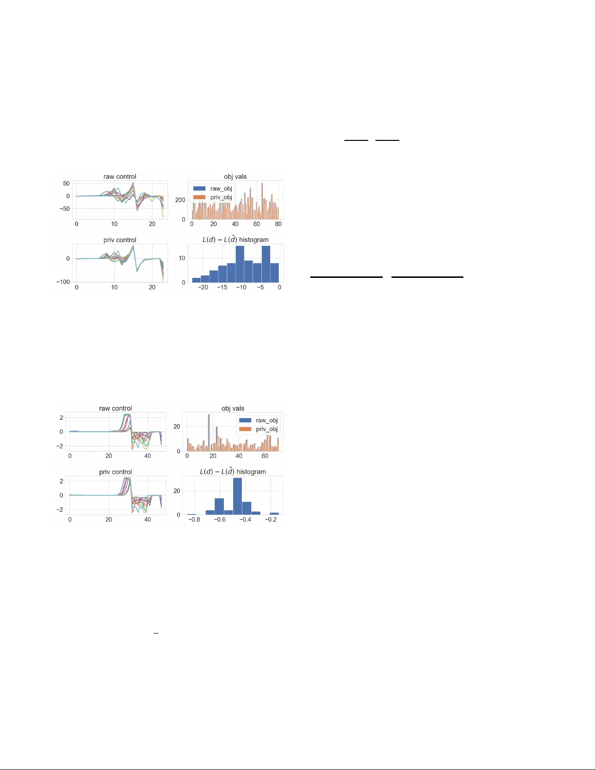
Ener gy Resource Control via Pri v ac y Preserving Data Xiao Chen † , Thomas Navidi ‡ , Ram Rajagopal † ‡ † Civil and Environmental Engineering, Stanford Univ ersity ‡ Electrical Engineering, Stanford University { markcx, tnavidi, ramr } @stanford.edu Abstract —Although the frequent monitoring of smart meters enables granular control over energy resources, it also increases the risk of leakage of private information such as income, home occupancy , and power consumption behavior that can be inferred from the data by an adversary . W e propose a method of releasing modified smart meter data so specific private attrib utes are obscured while the utility of the data f or use in an energy r esource controller is preserved. The method achieves priv atization by injecting noise conditional on the private attribute through a linear filter learned via a minimax optimization. The optimization contains the loss function of a classifier for the private at- tribute, which we maximize, and the energy resource controller’ s objective f ormulated as a canonical form optimization, which we minimize. W e perf orm our experiment on a dataset of household consumption with solar generation and another from the Commission for Energy Regulation that contains household smart meter data with sensitive attributes such as income and home occupancy . W e demonstrate that our method is able to significantly reduce the ability of an adversary to classify the private attribute while maintaining a similar objective value for an energy storage controller . Index T erms —Smart Meter , Pri vacy , Optimization, Battery Storage I . I N T RO D U C T I O N T raditionally , the power grid has been managed by the producers and grid operators with information primarily ex- changed among the large asset owners with little feedback from its end users. Howe ver , the push for renewable energy sources has brought about the rise of distributed energy resources (DERs) that lie under the control of many smaller and disparate users causing a paradigm shift in the flow of information in the grid. The successful operation of DERs and other smart grid technologies depends on the exchange of large amounts of data from many dif ferent end users [ 1 ]– [ 3 ]. Unfortunately , it may be unrealistic to assume the data will be a vailable without consideration of the pri vac y concerns the data owners may face. It has been demonstrated that the increased granularity of data required for smart grid operation enables the inference of personal information [ 4 ], which suggests data owners may be reluctant to exchange their data without some effort towards priv acy preservation. Studies ha ve in vestig ated various approaches to protect smart meter data pri vac y using a number of different met- rics. While detailed surveys are giv en in [ 5 ], [ 6 ], we briefly cov er a few popular solutions here. Aggregating data or its statistics has been considered [ 7 ], [ 8 ] to provide user priv acy since the aggregated data does not reflect any specific meter data above a certain aggregation size. Another approach at priv atization comes from dif ferential priv acy [ 9 ], which is widely adopted in pri v acy mechanism design and analysis in the context of energy data [ 10 ]–[ 14 ]. Specifically , studies [ 10 ], [ 11 ] and [ 12 ] proposed se veral framew orks for reducing the mutual information between raw data and priv atized data (e.g. po wer profiles). Approaches proposed in [ 13 ] in vestigated the differential priv acy effect with some noise injection (e.g. Laplace noise). It sho wed the aggregation group size must be of the order of thousands of smart meters in order to hav e reasonable utility . And [ 14 ] explored how much noise is required to be added to the data in order to achieve a certain lev el of dif ferential pri vac y for e xisting Laplace mechanism in the context of solving optimal power flow . W e distinguish our studies by focusing on developing a methodology that learns an optimal noise injection for bal- ancing the trade off between priv acy and data utility , thus, preserving as much utility in the data as possible. It differs from strict differential pri vac y because we use a general notion of priv acy that is the reduced correlation between priv ate attributes and the data. This general notion of priv acy gi ves us the flexibility to maintain the utility of the data while still eliminating an adversary’ s ability to recognize certain priv ate attributes. Since many applications of smart meter data in volve their use in optimization procedures, we define the utility as the performance achieved when such data is used for optimal control. W e consider a scenario where individual o wners of DERs, such as battery storage systems, wish to priv atize their data before releasing it to a DER aggregator to make optimal control decisions on their behalf, which can hav e applications in the context of [ 1 ], [ 2 ]. Our primary contributions are a minimax approach to gen- erate realistic meter data that is decorrelated from sensitive attributes while maintaining limited performance loss of a cost minimization optimal control algorithm using battery storage. Additionally , we de veloped a parallelized method that can be easily incorporated in modern deep learning architectures. The correlation of data priv atized by our method with sensitiv e attributes and the performance of a control algorithm is ev aluated on two real datasets of residential power demand: one with synthetic sensitiv e labels and one with real labels. W e demonstrate that our method is able to decrease the classification accuracy of an adversary by ov er 20% while maintaining the performance of the optimization to within 10% ov er both datasets. The rest of the paper is organized as follows: we describe the energy resource control in section II , control with pri- vatized data generated from the minimax learning algorithm in section III , experiments and results on the two datasets in section IV , and the Conclusion in Section section V . I I . E N E R G Y R E S O U R C E C O N T RO L A. Notation W e use bold letters for vectors and matrices and regular letters for scalars. Giv en two vectors x and y ∈ R n , x ≥ y represents the element-wise order x ( i ) ≥ y ( i ) for i ∈ [ n ] where [ n ] denotes the set [ n ] = { 1 , . . . , n } . And x ≥ 0 means all elements in the vector are not less than the scalar zero. W e make the dependence on the underlying probability distribution P when we write expectations (e.g. E P [ X ] where X denotes a random v ariable). The Frobenius norm of a matrix A is || A || F . W e write ∇ θ L ( θ ; X ) or d L ( θ ; X ) , where we typically mean differentiation of the loss function L with respect to the parameter θ ∈ R n . N stands for Normal (or Gaussian) distribution and R + denotes the non-negati ve real numbers. W e use := to represent ”define as. ” All the vectors are column vectors by default unless we explicitly address otherwise in a specific context. B. Battery storag e contr ol Control with deterministic demand : Consider a basic bat- tery control problem with the goal of minimizing the energy cost given a prescribed price p ∈ R H where H is the time horizon that is typically 24 if it is an hourly price. An uncontrollable electricity demand is specified as d ∈ R H + . W e denote the decision variables for battery control to be x and expand it into x in , x out , x s ∈ R H + that represents the charging, discharging, and the amount of charge in storage, i.e. x | = [ x | in , x | out , x | s ] . The battery optimal control is formulated as follows ( Problem 1 ): min x p | ( x in − x out + d ) + + β 1 || x in || 2 2 + β 2 || x out || 2 2 + β 3 || x s − αB || 2 2 (1a) s.t. x s ( j + 1) = x s ( j ) − 1 η out x out ( j ) + η in x in ( j ) ∀ j ∈ [ H ] (1b) x s (1) = B init (1c) 0 ≤ x in ≤ c in (1d) 0 ≤ x out ≤ c out (1e) 0 ≤ x s ≤ B . (1f) The linear term (with respect to x ) in the objectiv e is the cost of electricity when there is no v alue for selling the energy back to the grid. This represents a situation where there are no net- metering incentiv es. The quadratic penalty terms β 1 || x in || 2 2 and β 2 || x out || 2 2 are added to protect the battery state of health in the horizon [ 15 ]. The term β 3 || x s − αB || 2 2 is added to set the battery state to be close to the target value α B with B as the battery size and α ∈ (0 , 1) . β 1 , β 2 , β 3 are hyper -parameters to control these penalties. c in and c out are the char ging-in and discharging-out power capacities. And the parameter η in and η out denote the charging and discharging efficienc y (between 0 and 1). The constraint ( 1b ) indicates that the battery state in the next timestep equals the current battery state adding up the net charging amount (summing up charging and discharging together). Constraint ( 1c ) sets the initial state of the battery to have B init . T o simplify the notation, we define a set X := { x | ( 1b ) - ( 1f ) are feasible for some x ∈ R 3 H } . Hence, we use x ∈ X to succinctly e xpress that x satisfies the battery constraints. W e con vert the problem ( 1 ) into canonical con vex form in Appendix VI-B and de velop a paralleled algorithm making use of automatic differentiation, open-source conv ex solvers, and pytorch [ 16 ]–a popular deep learning framework. Control with stochastic demand : When determining the control with an uncertain demand, we minimize the expected cost under some demand distribution P . The objectiv e is slightly changed as follows ( Problem 2 ): min L u ( x , d ) := min x E d ∼ P  p | ( x in − x out + d ) +  + β 1 || x in || 2 2 + β 2 || x out || 2 2 + β 3 || x s − αB || 2 2 (2a) s.t. x ∈ X . (2b) I I I . C O N T RO L W I T H P R I V AT I Z ED D E M A N D Protecting priv acy in our context means reducing the corre- lation between the smart meter data and the sensitive attrib ute of the data owner , e.g. income or square-footage of the house. W e justify why such a consideration of priv acy protection is useful in practice in section III-A A. Revealing privacy fr om data In this section, we consider a simple scenario that the sensitiv e information is a binary label, such as a small or large home, which can be inferred from smart meter data. Giv en the ra w demand d ∈ R H + and sensiti ve label y ∈ { 0 , 1 } , the adversary builds a classifier f ψ that takes in demand d to estimate y with a prescribed loss function L a . Specifically , we assume the adversary minimizes the classification loss min ψ L a  f ψ ( d ) , y  to infer the pri vate information y. A popular choice of classi- fication loss is cross-entropy loss (or log-loss) [ 17 ] min ψ n − y log( f ψ ( d )) − (1 − y ) log  1 − f ψ ( d )  o when y is a binary variable. The classifier f ψ is parameterized by ψ and can be a neural network that outputs an estimate of the probability of the positive label. Previous studies [ 18 ], [ 19 ] showed that estimating a sensitiv e label such as income or square-footage of the house reaches 69% accuracy using features of smart meter data and models like support vector machine or random forest. W e use an alternativ e neural network model that leverages the daily power consumption (demand) and achieve state of the art accuracy of the priv ate label. More details can be found in section IV . B. Contr ol with private demand Our goal is to minimize energy cost incorporating of priv acy protection. Specifically , we design a data generator that creates a perturbed version of the raw demand data in a way that increases the adversarial classification loss, while enabling an optimal controller to minimize the energy cost. From a modeling perspective, we have a minimax problem ( Problem 3 ): min G L u  ˜ x ∗ ( ˜ d ) , d  − λ a L a ( f ( ˜ d ) , y ) (3a) s.t. ˜ d = d + G  ε y  , ε ∼ N (0 , I ) (3b) ˜ x ∗ ( ˜ d ) = arg min x ∈X L u ( x , ˜ d ) , (3c) where the parameter G is a matrix that af fects the distribution of ˜ d . In this case, we consider a linear transformation of Gaussian noise ε . V ariable y is the one-hot encoding of the sensitiv e binary label, and f ψ is a classifier that takes in the perturbed demand data and predicts the corresponding label priv ate label. The L u stands for utility loss. It is important to note that L u in the objectiv e uses the raw demand to ev aluate the cost of the control decisions determined using the perturbed demand. This represents the case where the storage unit acts on the perturbed information, but the real world v alue is based on the original raw data. In order to solve the non-trivial optimization ( 3 ), we sim- plify the constraints and make use of adversarial training that is further explained in section III-C , which is a common technique in studies of generativ e adversarial networks (GAN) and their applications [ 20 ], [ 21 ]. W e add a regularization term E || ˜ d − d || 2 2 in the objective with an additional hyper-parameter κ , min G L u  ˜ x ∗ ( ˜ d ) , d  − λ a L a ( f ( ˜ d ) , y ) + κ E || ˜ d − d || 2 2 , (4) which helps con vergence of the training and preserves parts of the demand that are not related to the pri v acy or utility loss instead of allowing them to be perturbed arbitrarily . W e can denote matrix G = [Γ , V ] with Γ ∈ R H × H and V ∈ R H × 2 . The altered demand then becomes ˜ d = d + Γ ε + V y . By denoting π to be the prior distribution of one-hot labels, e.g. π = [ p, 1 − p ] | where p is the prior probability of a positive label, we can rewrite the distortion regularization as E ( || ˜ d − d || 2 2 ) = E  || d + Γ ε + V y − d || 2 2  = E  (Γ ε + V y ) | (Γ ε + V y )  = E ( ε | Γ | Γ ε + y | V | V y + y | V | Γ ε + ε | Γ | V y ) (i) = E  T r(Γ εε | Γ | ) + T r( V y y | V | )  (ii) = T r(Γ E [ εε | | {z } I ]Γ T ) + T r    | | v 1 v 2 | |    p 2 p (1 − p ) p (1 − p ) (1 − p ) 2  | {z } E [ yy | ]  − v | 1 − − v | 2 −   (iii) = T r(ΓΓ | ) + || p v 1 + (1 − p ) v 2 || 2 2 = || Γ || 2 F + || V π || 2 2 (5) Equality (i) uses the fact that ε has zero mean. Equality (ii) expands out V as column vectors [ v 1 , v 2 ] and expresses E [ y y | ] = π π | = h p 1 − p i [ p 1 − p ] . Rearranging the expres- sions yields equality (iii). Therefore, we can equiv alently penalize the Frobenius norm of Γ and l 2 norm of the vector V π , i.e. || Γ || 2 F + || V π || 2 2 , instead of taking the empirical mean of the demand dif ference when performing the regularization. T o summarize, the data generator determines the filter weight G and outputs the perturbed demand ˜ d , while the adversary takes in the altered demand ˜ d and priv ate labels y to try to learn a classifier . C. Minimax learning W e construct two neural networks to perform the roles of the two players, one is for the data generator and the other one is for the adversary . T o train the adversary , we minimize the cross-entropy loss L a , i.e. min ψ L a  f ψ ( ˜ d ) , y  , which follo ws the loss function mentioned in section III-A . For the generator , we decouple the training into two steps. First, we le verage the loss that is passed from the adversary to update the matrix weight G = [Γ , V ] , i.e. ( step1 ) min G − λ a L a  f ψ  d + Γ ε + V y  , y  + κ  || Γ || 2 F + || V π || 2 2  (i) = min G =[Γ , V ] − λ a log  1 − f ψ  d + Γ ε + V y   + κ  || Γ || 2 F + || V π || 2 2  , (6) where κ is the hyper-parameter that penalizes the distance between ˜ d and d implicitly . Equality (i) uses the log-loss as the classification loss for the binary label. The next step is to use the priv atized demand ˜ d = d + b G h ε y i to determine the control by running the following optimization: ( step2 ) arg min x E ε ∼N (0 , I ) n p |  x in − x out + ˜ d  + + β 1 || x in || 2 2 + β 2 || x out || 2 2 + β 3 || x s − αB || 2 2 o (7a) s.t. x ∈ X . (7b) The optimal solution of the abov e con vex problem ( 7 ) is ˜ x ∗ , or more specifically ˜ x ∗ ( ˜ d ) , because it is a function of the priv atized demand, which is aligned with equation ( 3c ). The third step calculates the loss, L u ( ˜ x ∗ , d ) , using ˜ x ∗ ( ˜ d ) and the original raw demand expressed as: ( step3 ) L u ( ˜ x ∗ ( ˜ d ) , d ) = p |  ˜ x ∗ in ( ˜ d ) − ˜ x ∗ out ( ˜ d ) + d  + + β 1 || ˜ x ∗ in || 2 2 + β 2 || ˜ x ∗ out || 2 2 + β 3 || ˜ x ∗ s − αB || 2 2 . (8a) W e update G using gradient descent with the gradient determined by the chain rule. Recall that the generator outputs a priv atized demand with reduced correlation to the sensiti ve label that is also used to yield the storage control decisions. Those decisions are ev aluated on the cost given the raw demand, thus, the Jacobian of G is g G = ∇ G L u ( ˜ x ∗ , d ) = ∂ L u ( ˜ x ∗ , d ) ∂ x ∂ x ∂ ˜ d ∂ ˜ d ∂ G . (9) In the context of our storage control problem, the first term in ( 9 ) is ∂ L u ( x , d ) ∂ x =          Qx +    p − p 0    , if D x − d > 0 Qx otherwise , (10) where Q is giv en in the Appendix equation ( 21 ), I is the identity matrix, and D =  I − I 0  . The second term, i.e. ∂ x ∂ ˜ d , in ( 9 ) hinges on automatic differentiation through a conv ex program [ 22 ], [ 23 ]. Because an optimization problem can be vie wed as a function mapping the problem data to the primal and dual solutions, we can con vert problem ( 7 ) to a conic form and calculate the changes of the optimal solution given the perturbations of the problem data. It lev erages the idea of finding a zero solution for the residual map of a homogeneous self-dual embedding deriv ed from the KKT conditions of the con ve x program [ 23 ]–[ 25 ]. The third term in ( 9 ) is d G := ∂ ˜ d ∂ G = h d ˜ d ε 1 . . . d ˜ d ε H d ˜ d p d ˜ d 1 − p i ∈ R H × ( H +2) , (11) since d ˜ d = d G  ε y  . Thus, all three terms in equation ( 9 ) can be e valuated in the backward pass of the generator training and we can update the filter weight G using stochastic gradient decent [ 26 ]: G k +1 := G k − η l g G where k is the iteration step and η l is the learning rate. Remark : T o summarize, Step 1 sho wn in equation ( 6 ) updates the matrix G by minimizing the negati ve classification loss (equiv alent to maximizing the classification loss) of the ad- versary , while maintaining the constraint determined in ( 5 ). Step 2 calculates the optimal control of the storage using the priv atized demand. In Step 3, G is updated by ev aluating the gradient of the energy cost giv en the control based on the priv atized demand. The updates are expressed as ( update1 ) b G k +1 = G k − η ( k ) l ∇ G L a ( f ψ ( ˜ d ) , y ) (12a) ( update2 ) G k +1 = b G k +1 − η ( k ) l ∇ G L u ( ˜ x ∗ , d ) (12b) ( adversary update ) ψ k +1 = ψ k − η l ∇ ψ L a ( f ψ ( ˜ d ) , y ) , (12c) which run until con vergence. W e set the learning rates in each step to be equal for simplicity . The training procedure is described in Algorithm 1 . D. Con ver gence of the filter This subsection focuses on the stability and boundedness of the iterates in our back-propagation that lev erage stochas- tic gradient methods (or some related variants of first-order gradient methods). Using the subgradient property [ 27 , Chap- ter 9.1], g is a subgradient of f at x if f ( y ) ≥ f ( x ) + h g , y − x i ∀ y , (13) Algorithm 1: Minimax learning Input: Demand data D , label data Y , learning rate η l , parameters { B , α, β 1 , β 2 , β 3 } , and hyper parameters κ 1 , κ 2 Initialize G k , ψ k at iteration k = 0 with batch size m ; while ψ or G has not conver ged do 1 draw batches of pair ( d ( i ) , y ( i ) ) from demand and label datasets ( D , Y ), ∀ i = 1 , . . . , m ; 2 Sample batch of Gaussian random vectors ε (1) ,..., ( m ) ∼ N ( 0 , I ) ; 3 ψ k +1 := ψ k − η l E [ ∇ ψ L a ( f ψ ( ˜ d ) , y )] ; 4 b G k +1 := G k − η l E [ ∇ G L a ( f ψ ( ˜ d ) , y )] ; 5 G k +1 := b G k +1 − η l E [ ∇ G L u ( ˜ x ∗ , d )] where ˜ x ∗ is optimal solution of ( 7 ) (The expected gradient value is approximated as the sample mean of the batch.) retur n G and ψ and assuming G ∗ is a local optimal point; when we apply the step1 and step3 updates G k +1 = G k − η ( k ) l ∇L ( k ) a − η ( k ) l L ( k ) u at the k -th iteration, we can obtain the following relationship E [ || G k +1 − G ∗ || 2 2 ] (14a) = E [ || G k − η ( k ) l ( ∇L ( k ) a + ∇L ( k ) u ) − G ∗ || 2 2 ] (14b) = E [ || G k − G ∗ || 2 2 ] − 2 η ( k ) l E h∇L ( k ) a + ∇L ( k ) u , G k − G ∗ i + ( η ( k ) l ) 2 ||∇L ( k ) a + ∇L ( k ) u || 2 2 | {z } δ 2 k (14c) (i) = E [ || G k − G ∗ || 2 2 ] − 2 η ( k ) l E h∇L ( k ) a , G k − G ∗ i − 2 η ( k ) l E h∇L ( k ) u , G k − G ∗ i + ( η ( k ) l ) 2 δ 2 k (14d) (ii) ≤ E [ || G k − G ∗ || 2 2 ] − 2 η ( k ) l  L a ( G k ) − L ∗ a  − 2 η ( k ) l  L u ( G k ) − L ∗ u  + ( η ( k ) l ) 2 δ 2 k . (14e) Equality (i) expands the inner product of the loss gradients and iterates using δ k for the norm of the sum of loss gradients. The inequality (ii) uses the subgradient condition in equation ( 13 ), L ( G k ) − L ( G ∗ ) ≥ h∇L ( k ) , G k − G ∗ i (both for L a and L u ). Rearranging equation ( 14a ) and equation ( 14e ), we get 2 η ( k ) l  L a ( G k ) − L ∗ a  + 2 η ( k ) l  L u ( G k ) − L ∗ u  ≤ E [ || G k − G ∗ || 2 2 ] − E [ || G k +1 − G ∗ || 2 2 ] + ( η ( k ) l ) 2 δ 2 k . (15) By summing iterates up to step K , we get 2  K X k =1 η ( k ) l  min k ∈ [ k ] [ L a ( G k ) − L ∗ a ] + min k ∈ [ k ] [ L u ( G k ) − L ∗ u ] (16a) (iii) ≤ 2 K X k =1 η ( k ) l [ L a ( G k ) − L ∗ a ] + [ L u ( G k ) − L ∗ u ] (16b) (iv) ≤ || G 1 − G ∗ || 2 2 + K X k =1 ( η ( k ) l ) 2 δ 2 k (16c) where (iii) is valid since we take the minimum ov er all itera- tions and (i v) is deriv ed from the summation of equation ( 15 ). Then, arranging equation ( 16a ) and equation ( 16c ) gi ves min k ∈ [ k ] [ L 1 ( G k ) − L ∗ 1 ] + min k ∈ [ k ] [ L 2 ( G k ) − L ∗ 2 ] ≤ || G 1 − G ∗ || 2 2 + P K k =1 ( η ( k ) l ) 2 δ 2 k 2 P K k =1 η ( k ) l (17a) Thus, if the 2-norm of the vectorized version of G 1 − G ∗ is bounded by r , and with learning rate P k η ( k ) l − → ∞ but P k ( η ( k ) l ) 2 < ∞ , the right hand-side of equation ( 17a ) becomes r 2 + P k ( η ( k ) l ) 2 δ 2 k 2 P k η ( k ) l − → 0 . Therefore, using the gradient updates in step1 and step3 minimizes the losses L a , L u and con ver ges to a local optimal point. I V . E X P E R I M E N T S In this section, we ev aluate the capability of our linear filter to (1) generate perturbed smart meter data that reduces the prediction accuracy of sensitiv e attributes; (2) maintain the minimum energy cost from an optimal control decision using the perturbed data; (3) integrate into a contemporary deep learning architecture with parallelism. The code for our experiments is av ailable at https://github.com/ markcx/DER_ControlPrivateTimeSeries . A. Setup W e build up two neural networks to form the adversarial classifier and generator . The adv ersarial classifier is composed of two fully connected layers with ELU (Exponential Linear Unit) activ ation to estimate the sensiti ve attribute from de- mand. The first layer contains the same number of neurons as the time steps of the meter data series used by the battery optimal controller , and the second layer has half of the neuron numbers of the first layer and outputs a two dimensional vector representing the probability of the associated categories of the label. The generator module is composed of a single linear layer that takes a standard normal random vector and the priv ate labels as inputs, and outputs noise to be added to the original demand. The parameters of the single linear layer form matrix G . Additionally , we specify G to be block diagonal to reduce the number of learning parameters, i.e. G = [Γ , V ] where Γ is a diagonal matrix. Giv en the number of columns in our weight matrix is c w (e.g. the c w for G is 26 for the solar dataset and 50 in our residential experiments), we use uniform initialization [ 28 ] between ( − 1 c w , 1 c w ) for both the adversary and generator networks. W e use 85% of the data for training and the remaining 15% for testing the performance of the filter . W e set hyper -parameters β 1 = β 2 = β 3 = 10 − 5 , κ = 10 − 3 throughout the experiments. The learning rate for the classifier is 10 − 3 and the learning rate for the generator starts from 0 . 1 and decays 20% for every 100 steps. W e present the classification accuracy to indicate the correlation, as a lower accuracy implies a lower value of mutual information [ 29 ], thus, there is less correlation between the demand and sensitiv e labels. W e set the initial battery state of charge to 1% of its maximum energy capacity , i.e. B init = 0 . 01 B . W e use a time- of-use price structure with two tiers: a high price of $0.463 per KWh from 4pm-9pm and $0.202 per KWh for the rest of the day . B. Examples 1) Inte gration of storage and solar generation: For our first experiment, we aggregated 24-hour demand consumption from thousands of homes into groups of 100-200 homes and added solar generation. The aggregations represent the demand seen at a secondary transformer from the perspectiv e of a utility company . The goal is to minimize the energy cost by running the optimal charging and discharging controls for battery storage giv en a prescribed price. Each demand comes with a binary label indicating if the demand is from a high- or lo w-income group. W e wish to priv atize the demand before sending it to the storage operator to perform cost minimization, so the operator cannot infer any sensitiv e information from its customers. The left panel of Figure 1 shows the income attribute can be easily inferred from the raw demand as the height of the peaks are clearly distinguishable. The right panel of Figure 1 shows that the priv atized demands are perturbed such that two labels overlap making it harder to tell which demand has high or low income. Howe ver , there is a trade-off Fig. 1. A batch of 24-hour demand with solar generation that is net negativ e in certain hours allowing storage to minimize the cost through an optimal charge and discharge sequence. The left panel shows the raw demand. The right panel sho ws the privatized demand. between priv acy and utility when perturbing the data. W e use the hyper-parameter λ a to balance the adversarial loss and the utility loss i.e. smaller λ a means less weight for priv acy and more for utility , as shown in Figure 2 . When λ a increases from 8 to 128, the classification accuracy of the income label drops from 89.4% to 73% as we expected. The raw classification accuracy with zero weight is 95 . 2% . The loss of performance of the cost minimization by using priv atized demand instead of raw demand ranges from 5% at λ a = 8 to almost 10% at λ a = 128 on average, which shows that high priv acy comes with a performance cost for this battery control problem. 2) Deployment of storage on r esidential users: The second experiment considers residential customers adopting batteries to minimize their energy cost without selling excess to the grid. The control of the battery is performed by an outside program, so the o wner wishes to privatize their demand before sending it to the controller . The dataset is from the Irish CER Smart Metering Project [ 18 ], [ 30 ]. W e select a year of meter data for meters that contain a record indicating if they belong to a large or small home and partition it into daily sequences Fig. 2. The trade-off between priv acy and utility controlled by parameter λ a , which places weight on the priv ate attribute classification loss. with 48 entries for each day . W e end up with 54478 records in total. Recall that our goal is to create altered demand that won’ t degrade the cost sa vings while removing the correlation between the demand and the attribute indicating a small or large home. Figure 3 depicts the trade-off between utility degradation and priv acy gain for different weights on priv acy loss. The accuracy of classifying large or small homes based on the raw demand is 77.5%. When we hav e low weight on the priv acy loss (e.g. λ a = 0 . 5 ), the classification accuracy only drops a little to 75%, with a greater sacrifice on cost saving performance (e.g. increased to 8% more cost on av erage). In the high priv acy weight scenario, the classification accuracy drops down to 50% as desired, while the utility performance gap only increases up to 12%. Fig. 3. The trade-off between the utility and privac y for the CER dataset [ 30 ]. The privac y label indicates a large or small home. λ a weighs the privac y loss. C. P arallelism The experiments in this section are run on a six-core Intel Core i7 CPU @2.2GHz. Current standard solvers like Gurobi or Mosek without support of in-batch parallelism can be computationally expensiv e for solving a quadratic problem. Our filter makes use of automatic differentiation for a cone program (DIFFCP) [ 23 ] and leverages multiprocessing to speed up the forward and backward calculations. Figure 4 displays the mean and standard deviation of running each trial 8 times, showing that our batched module outperforms Gurobi or Mosek, which are highly tuned com- mercial solvers for reasonable batch sizes. For a minibatch size of 128, we solve all problems in an average of 1.31 seconds, whereas Gurobi takes an av erage of 11.7 seconds. This speed improvement for a single minibatch makes the difference between a practical and an unusable solver in the context of training a deep learning architecture. Fig. 4. CPU run time of a batched optimization using Gurobi v8.1.0, Mosek v8.1.0.60, and our parallel module. V . C O N C L U S I O N W e ha ve presented a method for the pri v atization of personal data that maintains its utility in the optimal control of energy resources. Our method comprises a small linear filter that adds random noise to the data conditional on the priv ate attributes we wish to protect. The linear filter is trained using a minimax optimization procedure that balances the trade-off between classifcation accuracy of the priv ate attributes and the performance of an optimal controller . Additionally , we include a distortion penalty to preserve aspects of the data that are not specified by the utility or priv acy functions in order to avoid adding arbitrary noise. W e have demonstrated that this method is capable of removing the correlation between the released priv ate data and the sensitive attributes while maintaining limited loss of the utility of the data using two datasets. Limitations of this method include the requirement to solve an optimization in the training loop, which can be computationally intensive for large problems; howe ver , we suspect only a few iterations of the optimization are needed to achiev e the desired gradients, which will dramatically reduce the computation required. V I . A P P E N D I X A. Battery contr ol details W e present a snapshot of the results for the storage control based on the raw and pri vate demand data. Figure 5 displays the storage control for our experiment with aggregated homes and solar generation. The upper-left and lower -left panel show the 24-hour charging and discharging decisions with each color representing one sample in a batch. The control decisions made with raw versus priv atized demand data are closely aligned in general, but hav e different charging and discharging amounts of power due to perturbation. Howe ver , such an altered charging profile doesn’t increase the minimum cost much as we can see from the upper-right and lower - right panels of Figure 5 . The electricity cost increases by a maximum of $22 USD per day giv en that the highest daily cost is around US $390 USD. (Each bin spans the range of $2.5 USD for Figure 5 .) Fig. 5. Analysis of storage control for the aggregated homes experiment with λ a = 128 . The upper - and lower -left panel show the charging and discharging power in kilowatts (KW). Different colored curves represent different samples in the batch. The upper-right panel shows the daily electricity cost when operating the battery using raw or priv ate demand (x- axis is the sample number, y-axis is in dollars ($)). The lower-right panel shows a histogram of the loss gap. (The x-axis is the increased cost in $; the y-axis is the number of days that show similar cost increases in a batch. ) Fig. 6. Analysis of storage control for the CER data experiment with λ a = 8 . Each panel has the same x- and y-axis as Figure 5 B. Quadratic pr oblem A canonical form of the quadratic constrained minimization problem (QP) is expressed as follows: min x 1 2 x T Qx + q T x (18a) s.t Ax = b (18b) Gx ≤ h. (18c) W e first show that the basic battery storage problem can be considered as a special case of QP . W e start with the 24- hour horizon storage problem in Problem 1 . W e can express the constraints from equation ( 1d ) to equation ( 1f ) as          I 0 0 − I 0 0 0 I 0 0 − I 0 0 0 I 0 0 − I − I I 0          | {z } G   x in x out x s   ≤          c in 0 c out 0 B 0 d          ⇔ Gx ≤ h. (19) W e add a constraint that the net of the demand and storage is greater than or equal to 0, so we can formulate the objectiv e as a QP . This constraint does not modify the original problem as long as it is feasible because the optimal solution will implicitly make the net of demand and storage greater than or equal to 0. The constraints in equation ( 1b )-equation ( 1c ) are expressed as  0 0 1 , . . . 0 [ η in I , 0] [ − 1 / η out I , 0] [ I , 0] − [0 , I ]  | {z } A   x in x out x s   =  B init 0  ⇔ Ax = b, (20) with [ I , 0] ∈ R 23 × 24 . The objective equation ( 1a ) can be con verted to a standard QP by letting Q =   β 1 I 0 0 0 β 2 I 0 0 0 β 3 I   , q =   p − p − 2 β 3 αB 1   . (21) Therefore, it is straightforward to discover that x T Qx + q T x is the new form of the objectiv e. R E F E R E N C E S [1] Andrey Bernstein and Emiliano Dall’Anese. Bi-lev el dynamic op- timization with feedback. In IEEE Global Conference on Signal and Information Pr ocessing (GlobalSIP) , Montreal, Canada, Nov ember 2017. [2] Y uanyuan Shi, Bolun Xu, Di W ang, and Baosen Zhang. Using battery storage for peak shaving and frequency re gulation: Joint optimization for superlinear gains. IEEE T ransactions on P ower Systems , 33:2882–2894, 2018. [3] Thomas Navidi, Abbas El Gamal, and Ram Rajagopal. A two-layer decentralized control architecture for der coordination. In 2018 IEEE Confer ence on Decision and Contr ol , pages 6019–6024, 2018. [4] Mikhail Lisovich, Deirdre Mulligan, and Stephen Wick er . Inferring per- sonal information from demand-response systems. Security & Privacy , IEEE , 8:11–20, 01 2010. [5] Marek Jawurek, Florian Kerschbaum, and George Danezis. Sok: Priv acy technologies for smart grids–a survey of options. Micr osoft Res., Cambridge, UK , 1:1–16, 2012. [6] Nikos Komninos, Eleni Philippou, and Andreas Pitsillides. Survey in smart grid and smart home security: Issues, challenges and countermea- sures. IEEE Communications Surveys & T utorials , 16(4):1933–1954, 2014. [7] Niklas Buescher, Spyros Boukoros, Stefan Bauregger , and Stefan Katzenbeisser . T wo is not enough: Privac y assessment of aggregation schemes in smart metering. Pr oceedings on Privacy Enhancing T ech- nologies , 2017(4):198–214, 2017. [8] Henry Corrigan-Gibbs and Dan Boneh. Prio: Pri vate, robust, and scal- able computation of aggregate statistics. In 14th { USENIX } Symposium on Networked Systems Design and Implementation ( { NSDI } 17) , pages 259–282, 2017. [9] Cynthia Dwork. Differential priv acy: A survey of results. In Manindra Agrawal, Dingzhu Du, Zhenhua Duan, and Angsheng Li, editors, Theory and Applications of Models of Computation , pages 1–19, Berlin, Heidelberg, 2008. Springer Berlin Heidelberg. [10] Lalitha Sankar, S Raj Rajagopalan, Soheil Mohajer, and H V incent Poor . Smart meter privac y: A theoretical framework. IEEE Tr ansactions on Smart Grid , 4(2):837–846, 2012. [11] Shuo Han, Ufuk T opcu, and George J Pappas. Ev ent-based information- theoretic priv acy: A case study of smart meters. In 2016 American Contr ol Confer ence (A CC) , pages 2074–2079. IEEE, 2016. [12] Jun-Xing Chin, T omas Tinoco De Rubira, and Gabriela Hug. Privac y- protecting energy management unit through model-distribution predic- tiv e control. IEEE Tr ansactions on Smart Grid , 8(6):3084–3093, 2017. [13] G ¨ unther Eibl and Dominik Engel. Differential privac y for real smart metering data. Computer Science-Research and Development , 32(1- 2):173–182, 2017. [14] F . Zhou, J. Anderson, and S. H. Low. Dif ferential privac y of aggregated dc optimal power flow data. In 2019 American Contr ol Conference (ACC) , pages 1307–1314, July 2019. [15] Mingxi Liu, Phillippe K Phanivong, and Duncan S Callaway . Customer- and network-aware decentralized ev charging control. In 2018 P ower Systems Computation Conference (PSCC) , pages 1–7. IEEE, 2018. [16] Adam Paszke, Sam Gross, Soumith Chintala, Gregory Chanan, Edward Y ang, Zachary DeV ito, Zeming Lin, Alban Desmaison, Luca Antiga, and Adam Lerer. Automatic differentiation in pytorch. NIPS 2017 W orkshop Autodif f Pr ogram , 2017. [17] Tsung-Y i Lin, Priya Goyal, Ross Girshick, Kaiming He, and Piotr Dollar . Focal loss for dense object detection. In The IEEE International Confer ence on Computer V ision (ICCV) , Oct 2017. [18] Christian Beckel, Leyna Sadamori, Thorsten Staake, and Silvia Santini. Rev ealing household characteristics from smart meter data. Ener gy , 78:397–410, 2014. [19] Xiao Chen, Peter Kairouz, and Ram Rajagopal. Understanding com- pressiv e adversarial privac y . In 2018 IEEE Confer ence on Decision and Contr ol (CDC) , pages 6824–6831. IEEE, 2018. [20] Ian Goodfellow , Jean Pouget-Abadie, Mehdi Mirza, Bing Xu, David W arde-Farley , Sherjil Ozair, Aaron Courville, and Y oshua Bengio. Gen- erativ e adversarial nets. In Advances in neural information pr ocessing systems , pages 2672–2680, 2014. [21] Y ize Chen, Xiyu W ang, and Baosen Zhang. An unsupervised deep learning approach for scenario forecasts. In 2018 P ower Systems Computation Confer ence (PSCC) , pages 1–7. IEEE, 2018. [22] Brandon Amos and J Zico Kolter . Optnet: Differentiable optimization as a layer in neural networks. In Pr oceedings of the 34th International Confer ence on Machine Learning-V olume 70 , pages 136–145. JMLR. org, 2017. [23] Akshay Agrawal, Shane Barratt, Stephen Boyd, Enzo Busseti, and W alaa M Moursi. Dif ferentiating through a conic program. Journal of Applied and Numerical Optimization , 1:107–115, 2019. [24] Y inyu Y e, Michael J T odd, and Shinji Mizuno. An o( √ nL )-iteration homogeneous and self-dual linear programming algorithm. Mathematics of Oper ations Resear ch , 19(1):53–67, 1994. [25] Enzo Busseti, W alaa M Moursi, and Stephen Boyd. Solution refinement at regular points of conic problems. Computational Optimization and Applications , pages 1–17, 2018. [26] L ´ eon Bottou. Large-scale machine learning with stochastic gradient descent. In Proceedings of COMPST AT’2010 , pages 177–186. Springer, 2010. [27] Stephen Boyd and Lieven V andenberghe. Con vex optimization . Cam- bridge uni versity press, 2004. [28] Kaiming He, Xiangyu Zhang, Shaoqing Ren, and Jian Sun. Delving deep into rectifiers: Surpassing human-lev el performance on imagenet classification. In Proceedings of the IEEE international conference on computer vision , pages 1026–1034, 2015. [29] Xiao Chen, Thomas Navidi, Stefano Ermon, and Ram Rajagopal. Dis- tributed generation of privac y preserving data with user customization. Safe Mac hine Learning workshop at ICLR , 2019. [30] Commission for Energy Regulation. Smart metering project-electricity customer behaviour trial, 2009-2010. http://www .ucd.ie/issda/data/ commissionforenergyre gulationcer/, 2012.