Using generative modelling to produce varied intonation for speech synthesis

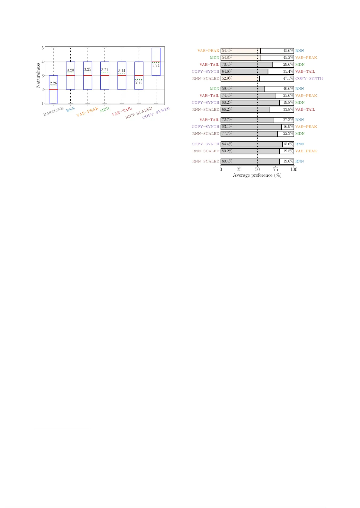
Using generativ e modelling to pr oduce varied intonation f or speech synthesis Zack Hodari, Oliver W atts, Simon King The Centre for Speech T echnology Research, Uni versity of Edinb ur gh, United Kingdom { zack.hodari, oliver.watts, Simon.King } @ed.ac.uk Abstract Unlike human speakers, typical text-to-speech (TTS) sys- tems are unable to produce multiple distinct renditions of a giv en sentence. This has pre viously been addressed by adding explicit external control. In contrast, generativ e models are able to capture a distribution ov er multiple renditions and thus pro- duce varied renditions using sampling. T ypical neural TTS models learn the average of the data because they minimise mean squared error . In the context of prosody , taking the av erage produces flatter , more boring speech: an “average prosody”. A generative model that can synthesise multiple prosodies will, by design, not model a ver - age prosody . W e use variational autoencoders (V AEs) which explicitly place the most “av erage” data close to the mean of the Gaussian prior . W e propose that by moving to wards the tails of the prior distribution, the model will transition towards generating more idiosyncratic, varied renditions. Focusing here on intonation, we in vestigate the trade-off be- tween naturalness and intonation v ariation and find that typical acoustic models can either be natural, or varied, but not both. Howe ver , sampling from the tails of the V AE prior produces much more varied intonation than the traditional approaches, whilst maintaining the same lev el of naturalness. Index T erms : speech synthesis, intonation modelling, prosodic variation, v ariational autoencoder, mixture density netw ork 1. Introduction Prosody in natural human speech varies predictably based on contextual factors. Howe ver , it also varies arbitrarily , or due to unknown factors [1]. T ext-to-speech (TTS) voices are typ- ically designed to synthesise a single most likely rendition of a giv en sentence. While many methods ha ve been proposed to add control to TTS voices, often they do not take this arbitrary variation into account. In contrast, we focus on designing TTS voices that are able to produce any viable prosodic realisation of a gi ven sentence in isolation. Such a system could be driv en by contextual information (e.g. provided by a dialogue system) to produce more appropriate prosodic renditions. Howe ver , we here focus on the task of producing random (but acceptable) prosodic renditions giv en an isolated sentence. Since neural statistical parametric speech synthesis (SPSS) became the leading paradigm in speech synthesis research [2] most TTS voices have used static plus dynamic features op- timised with mean squared error, followed by maximum like- lihood parameter generation (MLPG) and post-filtering [3]. These methods are a legac y of hidden Markov model (HMM) SPSS [4], where the problem of oversmoothing was observed and methods were developed to mitigate it. Oversmoothing of acoustic features is still an issue in neural SPSS, due to a com- bination of assumptions made in designing models [5]. Here we focus on prosody (and specifically on modelling intonation, which is the F 0 component of prosody) where the symptom of ov ersmoothing is flatter , more average prosody . W e argue that a model designed to synthesise distinct ren- ditions will, by design, not model av erage prosody . V ariational autoencoders (V AEs) are a class of generative models that can learn a smooth latent space approximating the true latent f actors of the data. Therefore, we use a V AE [6] to tackle the problem of a verage prosody , using the latent space to capture otherwise unaccounted-for variation. W e propose that by sampling from the low-probability regions of the V AE’ s prior we can generate idiosyncratic prosodic renditions. 2. Related work Methods for control of SPSS voices roughly fall into two cate- gories: explicitly labelled control and latent control. The former is typically expensiv e because labelling is labour-intensi ve, al- though this can be automated at the expense of accuracy [7, 8]. Labelling requires a concrete and consistent schema that can be followed by human annotators. For many aspects of variation in speech this is challenging, a clear example being emotion labelling [9]. For example, categorical emotions (e.g. happy or sad) may be too coarse, and appraisal-based measures (e.g. arousal or valence) may be too complex or ambiguous for la- bellers [10]. Additionally , there is the question of elicitation: should natural speech be annotated, or should the variation of interest be elicited (e.g., acted) and assumed to be correct? It has been sho wn that unsupervised methods can achieve similar results to supervised control [11], which may be related to the challenge of accurately labelling v ariation in real data, as discussed abov e. Discriminant condition codes, first proposed for speech recognition [12] hav e prov ed useful for multi-speaker TTS [13]. The same method has been applied in an unsupervised fashion [14], allowing for control of arbitrary v ariation. While these methods have been shown to have a probabilistic interpretation [11], they do not model uncertainty or guarantee smoothness in the latent space. As we discuss in Section 4, this smoothness is important for determining what corresponds to an idiosyncratic (and thus more varied) rendition of a sentence. T acotron [15] is a sequence-to-sequence model, for which style control using “global style tokens” (GST) has been pro- posed [16]. GSTs produce high quality speech, and can be pre- dicted from text [17]. Howe ver , individual GSTs cannot be ef- fectiv ely used to produce distinct styles as they are trained as weighted combinations; using individual GSTs leads to signif- icantly degraded audio quality . W e e xpect a random weighting of the tokens will also produce degraded naturalness, since there is no smoothness constraint. V AEs have been demonstrated for speech synthesis [18, 19], voice con version [20], and intonation modelling [21, Chap- ter 7]. Discrete representations hav e also been incorporated into the V AE framework [22, 23]. An experiment with VQ- V AE [23] demonstrated that phones can be learnt with unsuper- vised training, a result promising for potentially learning dis- crete prosodic styles. Howe ver , in this work we use a continu- ous latent space. The recently-introduced clockwork hierarchical V AE (CHiVE) [24] is similar to the model we propose here, how- ev er our V AE does not make use of the clockwork hierarchical structure and we only predict intonation, while CHiVE predicts F 0 , duration, and C 0 . Since we consider isolated sentences, we are not concerned with a single “best” output of our system. Prior work using V AEs has focused on modelling segmen- tal features [23, 18], with some applications to intonation mod- elling, e.g. for style transfer [24] and predicting latents from text [21, Chapter 7]. Ho wev er, our method mov es to wards TTS sys- tems that can synthesise multiple distinct prosodic renditions (in an unsupervised framew ork and without the need for control). 3. A verage prosody While many methods hav e been proposed to add control, there is a more fundamental issue, known as oversmoothing, which leads to flatter , more boring prosody . T ypical SPSS uses ei- ther feedforward neural networks, or recurrent neural networks (RNNs) to map from a linguistic specification to acoustic fea- tures. This mapping is learnt by minimising the mean squared error (MSE) against the ground truth acoustics. MSE is equiv a- lent to minimising the negati ve log-likelihood (NLL) of a unit- variance Gaussian. This has two effects on such SPSS models: they learn the mean of the data, and are sensiti ve to outliers. By modelling the mean, SPSS models over -smooth the acoustics – in the context of prosody this is kno wn as average pr osody . Methods such as the  -contaminated Gaussian [25] exist to handle outliers. Howe ver , to fix both issues, it is common to collect speech that is as controlled and consistent as possible in terms of style. T raining data with a single style results in models which produce more natural speech [26], but it also limits the voice’ s stylistic range. If we are interested in producing more varied style/prosody/intonation we need more varied data, but this must then be handled appropriately by our model. Generativ e models, such as Mixture density networks (MDN) [27], have the ability to handle multiple modes. MDNs parameterise a Gaussian mixture model (GMM) for each acous- tic frame which can help with oversmoothing of spectral fea- tures [28]. Howev er, for prosodic features, we are interested in fixing ov ersmoothing over a longer timescale, for which frame- lev el GMMs are less suitable. Instead, we use variational au- toencoders which model a distrib ution in an abstract (latent) space at whichev er timescale is preferred. 4. V ariational autoencoders V ariational autoencoders (V AEs) [6] are a class of latent vari- able models, i.e. they learn some unsupervised latent represen- tation of the data. They consist of an encoder and a decoder: the encoder parameterises the approximate posterior q φ ( z | x ) , which is an approximation of p θ ( z | x ) – the underlying f actors that describe the data. The decoder is trained to reconstruct the input signal x from this latent space, i.e. given a sample from the posterior ˜ z ∼ q φ ( z | x ) , we reconstruct ¯ x ∼ p θ ( x | ˜ z ) . The encoder and decoder are trained jointly by maximising the evidence lo wer bound (ELBO), L ( θ , φ ; x ) = − K L ( q φ ( z | x ) || p ( z )) + E q φ ( z | x ) [log p θ ( x | z )] (1) The first term in the ELBO enforces a prior on the approx- imate posterior , while the second term measures reconstruction error . The Kullback-Leibler (KL) div ergence term – used to en- force the prior – puts a cost on using the latent space. This cost on transmitting information through the latent space can encour- age the approximate posterior to collapse to the prior , thus en- coding no information: posterior collapse. KL-cost annealing is a common way to mitigate posterior collapse [29], where the KL term is down-weighted at the start of training, reducing the cost of encoding information in the latent space. Here we consider conditional V AEs [30], which model F 0 conditioned on linguistic features. W e use a sentence-level ap- proximate posterior , although a sequence of phrase- or syllable- lev el latents would be a reasonable alternative. W e use an isotropic Gaussian prior p ( z ) = N ( z ; 0 , 1 ) , which gives an analytical form of the KL term. Enforcing a Gaussian prior gi ves another useful quality: the single mode and smooth pdf means the distance of q φ ( z | x ) from the prior mean 0 will be in versely proportional to the sim- ilarity of x and the lar gest mode in the data (e.g., the most com- mon prosodic style). That is, the most idiosyncratic x will be far from the peak at 0 . This is helpful for our interest in varied prosodic renditions; we can generate varied prosodic renditions using the decoder by sampling lo w-density regions in the prior . Thus we define two models that use only the V AE decoder , z P E A K = 0 ¯ x P E A K ∼ p θ ( x | z P E A K ) (2) z TAI L ∼ v M F ( κ = 0) ¯ x TAI L ( r ) ∼ p θ ( x | r × z TAI L ) (3) where ¯ x P E A K should correspond to the most common mode, i.e. style. Due to the uni-modal prior p ( x ) , ¯ x P E A K may instead cor- respond to an average of multiple styles, i.e. a verage prosody . Our proposed model uses z TAI L (uniform samples on a hyper- sphere’ s surface 1 ) to produce idiosyncratic renditions ¯ x TAI L ( r ) , where the larger the radius r is the more unlikely the rendition. 5. Systems W e focus on modelling intonation, though in the future we plan to extend this to complete prosodic modelling (F 0 , duration and energy). Modelling only F 0 limits the range of variation we can achiev e, but reduces the risk of producing unnatural speech: spectral features and durations are taken from natural speech in our experiments, with full TTS left for future work. W e use the WORLD v ocoder [31], for analysis and synthesis. Our models 2 are implemented in PyT orch [32]. W e use the same basic recurrent architecture for all train- able modules in Figure 1: a feedforward layer with 256 units, followed by three uni-directional recurrent layers using gated recurrent cells (GR Us) [33] with 64 units, finally any outputs used are projected to the required output dimension. W e use 600-dimensional linguistic labels from the stan- dard Unilex question-set and 9 frame-lev el positional features with min-max normalisation as in the standard Merlin recipe [34]. The model predicts logF 0 , delta (velocity), and delta-delta (acceleration) features with mean-variance normalisation. W e use Adam [35] with an initial learning of 0.005, which is in- creased linearly for the first 1000 batches, and then decayed proportional to the in verse square of the number of batches [36, Sec 5.3], where our batch size is 32. Early stopping is used 1 Sampled from a von Mises-Fisher distribution ( vM F ) with uni- form concentration – wikipedia.org/wiki/V on MisesFisher distribution 2 Code is av ailable at github.com/ZackHodari/a verage prosody Acoustic Model F 0 F 0 Acoustic encoder F 0 V AE MDN Linguistic features Acoustic decoder  ( μ,σ ) Acoustic model Linguistic features F 0 RNN GMM  ( μ,σ ) 0 vMF (κ=0)*  F 0 V AE–PEAK Linguistic features Acoustic decoder Linguistic features F 0 V AE–TAIL Linguistic features Acoustic decoder Figure 1: Illustration of our models, wher e only the first thr ee ar e trained models. V A E – P E A K and V A E – TA I L are differ ent configurations of the V AE model. Blue: learned modules. Gr een: frame-level inputs. Orange: frame-level pr edictions. Y ellow: sentence-level latent space. based on v alidation performance. MLPG [37] is used to gener- ate the F 0 contour from the dynamic features; predicted standard deviations are used by the MDN, and all other models use the global standard deviation of the training data. The MDN uses four mixture components, whose variances are floored at 10 − 4 . T o synthesise from the MDN, we use the most likely component sequence (i.e. argmax) to select means and variances used in MLPG. Systems V A E – P E A K and V A E – TA I L in the list belo w are identical apart from the use of dif ferent sampling schemes (see Section 4). Their shared model uses a 16-dimensional isotropic Gaussian as the approximate posterior . The latent sample ˜ z is broadcast to frame-level and input to the decoder, along with the linguistic features. The decoder predicts static and dynamic logF 0 features; as such the reconstruction loss is MSE. The KL- div ergence term is weighted by zero during the first epoch and increased linearly to 0.01 over 40 epochs. Using this annealing schedule, the model con verged to a KL-di ver gence of 3.13. R N N Standard RNN-based SPSS model, using MSE. M D N MDN with 4 mixture components, using NLL. V A E – P E A K V AE decoder using z P E A K , i.e. the zero vector . V A E – TA I L V AE decoder using z TAI L with r = 3 , i.e. points on the surface of a hypersphere with radius 3. C O P Y – S Y N T H Natural F 0. BA S E L I N E A quadratic polynomial fitted to natural F 0 . R N N – S C A L E D F 0 from R N N , scaled vertically by a factor of 3. 5.1. Purpose of baselines BA S E L I N E sets a lower bound on naturalness (and variedness): no matter how much variation a system produces, its naturalness should nev er fall below that of B A S E L I N E . An upper-bound is C O P Y – S Y N T H : no system should be more natural than this, but might sound more varied ev en though it is unclear whether this would be fa voured by listeners. Because we expect that adding more variation will de grade naturalness, we wish to quantify this. R N N – S C A L E D is in- tended as a lower -bound on naturalness using a na ¨ ıve method for increasing variation, similar to v ariance scaling [38]. R N N – S C A L E D is intended to demonstrate that V A E – TAI L can produce the same amount of percei ved variation but without sacrificing as much naturalness. In this study , setting the amount of per - ceiv ed v ariation in R N N – S C A L E D and V A E – TA I L was calibrated in a pilot listening test by the authors, where we attempted to match the lev el of variation to C O P Y – S Y N T H . 6. Hypotheses H 1 V A E – TA I L will be much more varied than the typical SPSS systems ( R N N , V A E – P E A K , M D N ). H 2 R N N – S C A L E D , V A E – TAI L , and C O P Y – S Y N T H will have the same lev el of variedness . H 3 R N N , V A E – P E A K , and M D N will have a similar lev el of var - iedness , where M D N is more varied than the other two. H 4 V A E – TA I L will have slightly lower naturalness than the typical SPSS systems ( R N N , V A E – P E A K , M D N ). H 5 V A E – TA I L will be much more natural than the varied base- line R N N – S C A L E D . 7. Data Our choice of training data is motiv ated by the need for prosodic variation: if the data is v ery stylistically consistent, there will be too little variation for the V AE to capture in its latent space. W e therefore use the Blizzard Challenge 2018 dataset [39] pro vided by Usborne Publishing. The data consists of stories read in an expressi ve style for a 4–6 year old audience, with some charac- ter voices. Many of the stories include substantial amounts of direct speech. In total it contains 6.5 hours (~7,250 sentences) of professionally-recorded speech from a female speaker of standard southern British English. The training-validation-test split described in W atts et al. [14] is used. 8. Evaluation W e want to ev aluate the amount of variation produced by the systems described. Howe ver , v ariation alone is not a guarantee of “better” speech synthesis [40]. For this reason we ev aluate quality along with variation. T o determine quality we measure naturalness using a standard mean opinion score test, where users were asked to “rate the naturalness” on a 5-point Likert scale. Evaluating variation is less straightforward. W e employed a preference test where two systems were compared side by side for the same sentence. Users were asked to choose “which sen- tence has more v aried intonation”, where one sentence must be be marked as “more flat”, and the other as “more varied”. Due to the large number of pairs for 7 systems, we excluded B A S E - L I N E in the pairwise test, as it is clear from the speech samples 3 that it would be the least varied. Howe ver , without BA S E L I N E in the variation test we lose our lo wer-bound on v ariation. W e randomly selected 32 test sentences of between 7 and 11 words (1.4 to 4.8 seconds). The naturalness test was performed before the preference test. As there were 22 screens to be com- pleted for each sentence it was necessary to split the test into two halves using a simple 2x2 Latin square between-subjects design. In total we used 30 participants, 15 per listener group, the test took 45 minutes and participants were paid £8. 9. Results 9.1. Naturalness test A summary of the naturalness ratings is provided in Figure 2. W e perform a Wilcoxon rank-sums significance test between all pairs of systems in the naturalness test, followed by Holm- Bonferroni correction. This statistical analysis is the same as for the Blizzard challenge [41]. V A E – TA I L , R N N , M D N , and V A E – P E A K form a group for which we did not find any significant 3 Speech samples a vailable at github.com/ZackHodari/a verage prosody baseline rnn v ae–peak mdn v ae–t ail rnn–scaled copy–synth 1 2 3 4 5 Naturalness 2.26 3.20 3.25 3.21 3.14 2.73 3.94 Figure 2: Naturalness r esults. Solid red lines ar e medians, dashed gr een lines are means (cannot be used for statistical comparison), blue boxes show the 25 th and 75 th per centiles, and whiskers show the range of the ratings, excluding outliers which ar e plotted with + . Order ed accor ding to the variation test. difference. All other system pairs are significantly different, with a corrected p-value of less than 0.00001. 9.2. V ariation test While it is not guaranteed that human preferences are self- consistent, or globally consistent 4 , we see that the results in Figure 3 do form a consistent ordering from most flat to most varied: R N N → V A E – P E A K → M D N → V A E – TAI L → C O P Y – S Y N T H → R N N – S C A L E D . Howe ver , relative variedness is sometimes inconsistent, e.g. while R N N – S C A L E D is more v ar- ied than C O P Y – S Y N T H (5 th row), we see that the difference be- tween C O P Y – S Y N T H and R N N (13 th row) is greater than the dif- ference between R N N – S C A L E D and R N N (15 th row). W e perform a binomial significance test for the 15 pairs in the listening test, followed by Holm-Bonferroni correction. W ith the correction we find that ( R N N , V A E – P E A K ), ( V A E – P E A K , M D N ), and ( C O P Y – S Y N T H , R N N – S C A L E D ) did not show a significant difference: this is indicated by the colouring of those pairs in Figure 3. All other pairs are significantly differ - ent, with a corrected p-value of less than 0.0002. 9.3. Naturalness–V ariedness trade-off While this ordering supports our expectations, we cannot clearly comment on their support of our h ypotheses in Section 6 as the relati ve variedness between systems is not clear . Addi- tionally , we w ould like to clearly compare the trade-of f between increasing intonation variation and naturalness. This requires us to represent the pairwise preferences in Figure 3 along a single axis. W e could approach this using multi-dimensional scaling (MDS) [43]; howe ver , the pairwise preferences correspond to directed edges, not distances. Instead, we formulate the prob- lem as a system of linear equations 5 . Here, the variables are the positions of each system in the dimension of relativ e var- iedness, and each equation describes the “excess preference” of a system pair (the difference between the two system’ s aver - age preference). This system can be solved using ordinary least squares: Ax = b x = ( A T A ) − 1 A T b 4 As described by Arrow’ s impossibility theorem [42]. 5 W e thank Erfan Loweimi and Gustav Henter for insightful discus- sions that led to this formulation of the problem. 0 25 50 75 100 Av erage preference (%) rnn–scaled rnn 80.4% 19.6% rnn–scaled v ae–peak 80.2% 19.8% copy–synth rnn 84.4% 15.6% rnn–scaled mdn 77.7% 22.3% copy–synth v ae–peak 83.1% 16.9% v ae–t ail rnn 72.7% 27.3% rnn–scaled v ae–t ail 66.2% 33.8% copy–synth mdn 80.2% 19.8% v ae–t ail v ae–peak 74.4% 25.6% mdn rnn 59.4% 40.6% rnn–scaled copy–synth 52.9% 47.1% copy–synth v ae–t ail 64.6% 35.4% v ae–t ail mdn 70.4% 29.6% mdn v ae–peak 54.8% 45.2% v ae–peak rnn 54.4% 45.6% Figure 3: P airwise variedness r esults. P airs ar e or dered such that the more varied system is on the left. The top 5 r ows give the pairs that are consecutive in the or dering, with following r ows showing systems that ar e incr easingly further apart in the or dering. W e did not find a significant differ ence for the pairs marked in a lighter colour . where A ∈ {− 1 , 0 , 1 } 15 × 6 and b ∈ R 15 × 1 encode the pairwise results in Figure 3. Gi ven the solution ( x ∈ R 6 × 1 ) we plot naturalness against relativ e variedness in Figure 5. Systems to the left hav e flatter intonation, and systems to the right have more v aried intonation. This axis represents human preference and is not intended to be a perceptual scale. In Figure 5, we see that V A E – TAI L is much more varied than the typical SPSS systems ( H 1 ). It is also clear that our cali- bration fav oured less v ariation in V A E – TA I L than C O P Y – S Y N T H (rejecting H 2 ), thus we cannot mak e broad statements about the naturalness-variedness trade-of f. Howe ver , based on the signif- icant drop in naturalness from R N N to R N N – S C A L E D , and the clustering over relativ e variedness, we believ e that V A E – TA I L would still be significantly more natural than R N N – S C A L E D ev en if it matched C O P Y – S Y N T H ’ s lev el of variation. R N N , V A E – P E A K , and M D N are clustered along the axis of relativ e variation, with MD N being significantly more varied, but only by a small amount ( H 3 ). Demonstrating that all systems suffer from o versmoothing of F 0 to a similar extent. While the mean naturalness of V A E – TA I L is lower than R N N , V A E – P E A K , and M D N , the means cannot be directly com- pared, and no significant difference was found in Section 9.1. Rejecting H 4 suggests we can produce more varied intonation without sacrificing naturalness. Ho wever , we expect that with the ideal calibration we may see some slight de gradation in nat- uralness of V A E – TA I L . W e do observe that V A E – TA I L is much more natural than R N N – S C A L E D ( H 5 ). 10. Analysis Calibration The horizontal axis in Figure 5 sho ws V A E – TAI L having much greater percei ved intonation variation than M D N , while the logF 0 histograms in Figure 4 shows them as having 54 148 403 0 2000 4000 baseline 54 148 403 rnn 54 148 403 v ae–peak 54 148 403 mdn 54 148 403 v ae–t ail 54 148 403 rnn–scaled 54 148 403 copy–synth F0 (Hz) – log scale Figure 4: Histogram of logF 0 values for each system over all the listening test material. Or dered accor ding to the variation test. Relativ e v ariedness 1 2 3 4 5 Mean naturalness rnn v ae–peak mdn v ae–t ail rnn–scaled copy–synth baseline flat v aried ← − − → Figure 5: Naturalness-variedness trade-off. Ideally as we in- cr ease the amount of pr osodic variation our system will not de- cr ease in naturalness. Note that naturalness comparisons can only be made using the significance r esults in Section 9.1. the same amount of objectiv e variation – variance of logF 0 pre- dictions for the listening test stimuli. This demonstrates that objectiv e measures do not necessarily correspond to perceived variation, which is exactly what makes calibration of V A E – TA I L and R N N – S C A L E D difficult. Figure 4 shows that V A E – TA I L has a narrower histogram than C O P Y – S Y N T H , howev er as objective measures do not necessarily correspond to perceived variation we chose not to rely on objectiv e measures for calibration. Multiple renditions W e have demonstrated the ability to pro- duce varied intonation while maintaining the same level of nat- uralness, thus mitigating average prosody . Howe ver , we have not demonstrated V A E – TA I L ’ s ability to produce multiple dis- tinct prosodic renditions. In Figure 6 we present a density of 10,000 F 0 contours ¯ x TAI L (3) produced using samples z TAI L ∼ v M F ( κ = 0) . As expected, the F 0 contours produced vary smoothly , but more importantly we see that they vary between multiple distinct contours. F or this sentence we see that there may be three distinct contours. W e are interested in ev aluat- ing the distincti veness of multiple different samples from V A E – TAI L ; howe ver , this is out of the current scope. MDN sampling While M D N is also a generati ve model, sampling from the frame-lev el GMMs is not straightforward. MLPG can be used to select the single best trajectory [37, Case 3]. But to produce multiple renditions from M D N we must choose a sequence of Gaussian components. Howe ver , ran- domly choosing components produces noisy F 0 contours, and using the same component for the entire sequence does not pro- 0.0 0.5 1.0 1.5 2.0 2.5 3.0 Time (s) 0 50 100 150 200 250 300 350 400 F0 (Hz) Figure 6: Density of F 0 pr edictions made by V A E – TA I L for the sentence ”Goldilocks skipped ar ound a corner and saw ... ” duce distinct performances. This is likely because the compo- nents don’t represent modes of the data, but beha ve in a similar way to the  -contaminated Gaussian distrib ution [25]. 11. Conclusion W e hav e demonstrated that output from typical RNN and MDN models exhibits flat intonation. Additionally , we hav e provided evidence that sampling from the tails of a V AE prior produces speech that is much more varied than typical SPSS while main- taining the same lev el of naturalness. In future we plan to un- dertake a full evaluation of this trade-off, to determine if and when this method begins to impro ve or de grade in quality . In future work, we plan to: use MUSHRA in place of a pref- erence test; use a neural vocoder; make use of seq2seq models with attention instead of upsampling the linguistic features; pre- dict other prosodic features; and make use of either a discrete latent space [22] or a mixture model V AE prior [44]. Acknowledgements: Zack Hodari w as supported by the EPSRC Centre for Doctoral T raining in Data Science, funded by the UK Engineering and Physical Sciences Research Council (grant EP/L016427/1) and the Univ ersity of Edinburgh. Oli ver W atts was supported by EPSRC Stan- dard Research Grant EP/P011586/1. 12. References [1] Y . Xu, “Speech prosody: A methodological revie w , ” Journal of Speech Sciences , v ol. 1, no. 1, pp. 85–115, 2011. [2] S. King, “Measuring a decade of progress in te xt-to-speech, ” Lo- quens , vol. 1, no. 1, p. 6, 2014. [3] H. Zen, A. Senior , and M. Schuster, “Statistical parametric speech synthesis using deep neural networks, ” in Pr oc. ICASSP . V an- couver , Canada: IEEE, 2013, pp. 7962–7966. [4] H. Zen, K. T okuda, and A. W . Black, “Statistical parametric speech synthesis, ” Speech Communication , vol. 51, no. 11, pp. 1039–1064, 2009. [5] G. E. Henter, T . Merritt, M. Shannon, C. Mayo, and S. King, “Measuring the perceptual effects of modelling assumptions in speech synthesis using stimuli constructed from repeated natural speech, ” in Pr oc. Interspeech , Singapore, 2014, pp. 1504–1508. [6] D. P . Kingma and M. W elling, “ Auto-encoding variational Bayes, ” arXiv pr eprint arXiv:1312.6114 , 2013. [7] A. Rosenberg, “AuT oBI - a tool for automatic T oBI annotation, ” in Pr oc. Interspeech , Makuhari, Japan, 2010, pp. 146–149. [8] Z. Hodari, O. W atts, S. Ronanki, and S. King, “Learning inter- pretable control dimensions for speech synthesis by using external data, ” in Pr oc. Interspeech , Hyderabad, India, 2018, pp. 32–36. [9] E. Douglas-Co wie, N. Campbell, R. Cowie, and P . Roach, “Emo- tional speech: T owards a new generation of databases, ” Speech Communication , vol. 40, no. 1, pp. 33–60, 2003. [10] Z. Hodari, “ A learned emotion space for emotion recognition and emotiv e speech synthesis, ” Master’s thesis, The University of Ed- inbur gh, 2017. [11] G. E. Henter, J. Lorenzo-T rueba, X. W ang, and J. Y amagishi, “Deep encoder-decoder models for unsupervised learning of con- trollable speech synthesis, ” arXiv preprint , 2018. [12] S. Xue, O. Abdel-Hamid, H. Jiang, L. Dai, and Q. Liu, “Fast adaptation of deep neural network based on discriminant codes for speech recognition, ” IEEE Tr ans. on Audio, Speech and Lan- guage Pr ocessing , vol. 22, no. 12, pp. 1713–1725, 2014. [13] H.-T . Luong, S. T akaki, G. E. Henter, and J. Y amagishi, “ Adapting and controlling DNN-based speech synthesis using input codes, ” in Pr oc. ICASSP . New Orleans, USA: IEEE, 2017, pp. 4905– 4909. [14] O. W atts, Z. W u, and S. King, “Sentence-lev el control vectors for deep neural network speech synthesis, ” in Pr oc. Interspeech , Dresden, Germany , 2015, pp. 2217–2221. [15] Y . W ang, R. Skerry-Ryan, D. Stanton, Y . W u, R. J. W eiss, N. Jaitly , Z. Y ang, Y . Xiao, Z. Chen, S. Bengio et al. , “T acotron: T owards end-to-end text-to-speech synthesis, ” arXiv preprint arXiv:1703.10135 , 2017. [16] Y . W ang, D. Stanton, Y . Zhang, R. Skerry-Ryan, E. Battenberg, J. Shor, Y . Xiao, F . Ren, Y . Jia, and R. A. Saurous, “Style tokens: Unsupervised style modeling, control and transfer in end-to-end speech synthesis, ” arXiv pr eprint arXiv:1803.09017 , 2018. [17] D. Stanton, Y . W ang, and R. Skerry-Ryan, “Predicting expressiv e speaking style from text in end-to-end speech synthesis, ” arXiv pr eprint arXiv:1808.01410 , 2018. [18] W .-N. Hsu, Y . Zhang, R. W eiss, H. Zen, Y . W u, Y . Cao, and Y . W ang, “Hierarchical generative modeling for controllable speech synthesis, ” in Pr oc. ICLR , New Orleans, USA, 2019. [19] K. Akuzawa, Y . Iwasaw a, and Y . Matsuo, “Expressive speech synthesis via modeling e xpressions with variational autoencoder , ” arXiv pr eprint arXiv:1804.02135 , 2018. [20] C.-C. Hsu, H.-T . Hwang, Y .-C. W u, Y . Tsao, and H.-M. W ang, “V oice con version from unaligned corpora using variational au- toencoding wasserstein generativ e adversarial networks, ” arXiv pr eprint arXiv:1704.00849 , 2017. [21] X. W ang, “Fundamental frequency modelling for neural-network- based statistical parametric speech synthesis, ” Ph.D. dissertation, SOKEND AI – The Graduate University for Advanced Studies, 2018. [22] J. T . Rolfe, “Discrete variational autoencoders, ” arXiv preprint arXiv:1609.02200 , 2016. [23] A. v an den Oord, O. V inyals et al. , “Neural discrete representation learning, ” in Proc. NeurIPS , Long Beach, USA, 2017, pp. 6306– 6315. [24] V . W an, C.-a. Chan, T . Kenter , J. Vit, and R. Clark, “CHiVE: V arying prosody in speech synthesis with a linguistically driven dynamic hierarchical conditional variational network, ” in Proc. ICML , Long Beach, USA, 2019. [25] H. Zen, Y . Agiomyrgiannakis, N. Egberts, F . Henderson, and P . Szczepaniak, “Fast, compact, and high quality LSTM-RNN based statistical parametric speech synthesizers for mobile de- vices, ” in Pr oc. Interspeech , San Francisco, USA, 2016, pp. 2273– 2277. [26] M. Podsiadlo and V . Ungureanu, “Experiments with training cor- pora for statistical text-to-speech systems, ” in Pr oc. Interspeech , Hyderabad, India, 2018, pp. 2002–2006. [27] C. M. Bishop, “Mixture density networks, ” Citeseer , T ech. Rep., 1994. [28] H. Zen and A. Senior , “Deep mixture density networks for acous- tic modeling in statistical parametric speech synthesis, ” in Pr oc. ICASSP . Florence, Italy: IEEE, 2014, pp. 3844–3848. [29] I. Higgins, L. Matthey , A. Pal, C. Burgess, X. Glorot, M. Botvinick, S. Mohamed, and A. Lerchner , “ β -V AE: Learning basic visual concepts with a constrained v ariational frame work, ” in Pr oc. ICLR , vol. 3, T oulon, France, 2017. [30] K. Sohn, H. Lee, and X. Y an, “Learning structured output rep- resentation using deep conditional generativ e models, ” in Proc. NeurIPS , Montreal, Canada, 2015, pp. 3483–3491. [31] M. Morise, F . Y okomori, and K. Ozaw a, “WORLD: A v ocoder- based high-quality speech synthesis system for real-time appli- cations, ” IEICE T rans. Inf. Syst. , vol. 99, no. 7, pp. 1877–1884, 2016. [32] A. Paszke, S. Gross, S. Chintala, G. Chanan, E. Y ang, Z. DeV ito, Z. Lin, A. Desmaison, L. Antiga, and A. Lerer , “ Automatic differ - entiation in PyT orch, ” in NIPS-W , Long Beach, USA, 2017. [33] K. Cho, B. V an Merri ¨ enboer , C. Gulcehre, D. Bahdanau, F . Bougares, H. Schwenk, and Y . Bengio, “Learning phrase rep- resentations using RNN encoder -decoder for statistical machine translation, ” arXiv pr eprint arXiv:1406.1078 , 2014. [34] Z. W u, O. W atts, and S. King, “Merlin: An open source neu- ral network speech synthesis system, ” in Proc. Speech Synthesis W orkshop , Sunnyvale, USA, 2016, pp. 124–124. [35] D. Kingma and J. Ba, “ Adam: A method for stochastic optimiza- tion, ” arXiv pr eprint arXiv:1412.6980 , 2014. [36] A. V aswani, N. Shazeer, N. Parmar, J. Uszkoreit, L. Jones, A. N. Gomez, Ł. Kaiser, and I. Polosukhin, “ Attention is all you need, ” in Pr oc. NeurIPS , Long Beach, USA, Dec 2017, pp. 5998–6008. [37] K. T okuda, T . Y oshimura, T . Masuko, T . Kobayashi, and T . Kita- mura, “Speech parameter generation algorithms for HMM-based speech synthesis, ” in Proc. ICASSP , vol. 3. Istanbul, T urkey: IEEE, 2000, pp. 1315–1318. [38] H. Sil ´ en, E. Helander, J. Nurminen, and M. Gabbouj, “W ays to implement global variance in statistical speech synthesis, ” in Pr oc. Interspeech , Portland, USA, 2012, pp. 1436–1439. [39] S. King, J. Crumlish, A. Martin, and L. Wihlborg, “The Blizzard challenge 2018, ” in Proc. Blizzar d Challenge W orkshop , Hyder- abad, India, 2017. [40] J. Latorre, K. Y anagisawa, V . W an, B. K olluru, and M. J. Gales, “Speech intonation for TTS: Study on evaluation methodology , ” in Pr oc. Interspeech , Singapore, 2014, pp. 2957–2961. [41] R. A. Clark, M. Podsiadlo, M. Fraser, C. Mayo, and S. King, “Statistical analysis of the Blizzard challenge 2007 listening test results, ” in Proc. Blizzard Challenge W orkshop , Bonn, Germany , 2007. [42] K. J. Arrow , “ A dif ficulty in the concept of social welfare, ” J. of political economy , vol. 58, no. 4, pp. 328–346, 1950. [43] I. Borg and P . Groenen, “Modern multidimensional scaling: Theory and applications, ” Journal of Educational Measurement , vol. 40, no. 3, pp. 277–280, 2003. [44] J. M. T omczak and M. W elling, “V AE with a V ampPrior, ” in Proc. Artificial Intelligence and Statistics , Lanzarote, Spain, 2018, pp. 1214–1223.