The Probabilistic Backbone of Data-Driven Complex Networks: An example in Climate
Correlation Networks (CNs) inherently suffer from redundant information in their network topology. Bayesian Networks (BNs), on the other hand, include only non-redundant information (from a probabilistic perspective) resulting in a sparse topology fr…
Authors: Catharina Graafl, Jose M. Gutierrez, Juan M. Lopez
The Pr obabilistic Bac kbone of Data-Driven Comple x Netw orks: An e xample in Climate * Catharina E. Graafland 1,* , Jos ´ e M. Guti ´ errez 1 , Juan M. L ´ opez 1 , Diego P az ´ o 1 , and Miguel A. Rodr ´ ıguez 1 1 Instituto de F ´ ısica de Cantabria, CSIC–Universidad de Cantabria, A venida de Los Castros , E-39005 Santander , Spain * catharina.graafland@unican.es ABSTRA CT Comple x systems often e xhibit long-range correlations so that typical observab les show statistical dependence across long distances. These teleconnections hav e a tremendous impact on the dynamics as they pro vide channels for inf ormation transpor t across the system and are par ticularly relev ant in forecasting, control, and data-driven modeling of comple x systems. These statistical interrelations among the v er y many degrees of freedom are usually represented b y the so-called correlation network, constructed by establishing links between v ariables (nodes) with pairwise correlations abov e a given threshold. Here, with the climate system as an e xample, we revisit correlation networks from a probabilistic perspective and show that the y unav oidably include m uch redundant information, resulting in overfitted probabilistic (Gaussian) models . As an alter native, w e propose here the use of more sophisticated probabilistic Bay esian networks, dev eloped by the machine learning community , as a data-driven modeling and prediction tool. Bay esian networks are b uilt from data including only the (pairwise and conditional) dependencies among the v ariables needed to e xplain the data ( i.e. , maximizing the lik elihood of the underlying probabilistic Gaussian model). This results in much simpler, sparser , non-redundant, networks still encoding the comple x structure of the dataset as re vealed by standard complex measures. Moreov er , the networks are capab le to generaliz e to new data and constitute a truly probabilistic bac kbone of the system. When applied to climate data, it is shown that Bay esian networks f aithfully rev eal the various long-range teleconnections rele vant in the dataset, in particular those emerging in El Niño per iods. Introduction Due to the widespread interest of the scientific community in data science, an increasing body of research in the field of complex networks is now focusing on the de velopment of graph machine learning algorithms for analysis and prediction 1 . Some rele v ant applications include link prediction 2 , 3 , network embedding 4 , pattern mining 5 , and graph neural networks 6 . Most of this research is currently oriented towards the application of deep learning methods 7 – 10 . Howe ver , there are a number of traditional machine learning methods that could be used in the modern context of complex graph analytics and prediction. For instance, Bayesian network (BN) models 11 are a sound and popular machine learning technique used to b uild tractable probabilistic models from data using auxiliary graphs— representing the most relev ant (pairwise and conditional) dependencies among the variables needed to e xplain the data as a whole (maximizing the likelihood of the underlying Gaussian model). These models hav e been successfully applied in a few particular climate applications, such as probabilistic weather prediction 12 or causal teleconnection analysis 13 , 14 . In recent years, the most popular approach to modeling and obtain the patterns of teleconnections in complex systems, like for instance climate, is based on correlation netw orks (CNs) 15 – 22 . The difference between CNs and BNs is that, whereas the former are exclusi vely b uilt considering pairwise dependencies ( e.g. , correlations) between v ariables (based on the choice of an arbitrary threshold), the latter use more sophisticated learning methods to model also conditional dependencies, i.e. , dependencies between two (sets of) v ariables, given a third (set). Here we sho w that this results in sparser , non-redundant, networks with a complex topology , including a maximal entropy community structure. Moreover , as we shall sho w here, from a probabilistic perspecti ve CNs and BNs lead to very dif ferent empirical Gaussian models. The resulting CN distrib ution function is either too simple (mostly dominated by local information, therefore, unable to predict teleconnection patterns for high correlation threshold values) or too noisy (containing too man y parameters for small thresholds) and prone to overfitting. In contrast, the BN distribution function is a parsimonious representation suitable for analysis and probabilistic inference. Summarizing, we shall adv ocate here the use of BNs as non-redundant graph representations of complex data, suitable for probabilistic modeling and analysis with complex netw ork measures. For the case of climate data 23 , we shed light on the * This is a pre-print of an article published in Scientific Reports. The final authenticated version is av ailable online at: https://doi.org/10.1038/s41598-020- 67970-y . construction of the proposed BNs and compare with the usual CNs approach by characterizing the topology of both type of networks. This graph theoretic analysis sho ws why CN topologies are inherently redundant, while BNs are not. Moreover , by using machine learning techniques, we analyse the networks as Probabilistic Graphical Models (PGMs) that ha ve objecti ve information content to soundly present the underlying Gaussian model. It will become clear that redundancy in topology is associated with the surge of meagre model parameters, so that this redundancy hinders the use of CNs to extrapolate meaningful features in the case of ne w data. W e illustrate this with a particular e xtrapolation study in which we query the networks to predict the teleconnections that appear during a climatic ev ent (El Niño). Results Climate network construction The construction of CNs and BNs in climate is illustrated using a global temperature dataset previously used in many studies 16 , 17 , 21 that shows well-kno wn properties characterized by the interplay of strong local and weak long-distant (telecon- nections) dependencies. In particular , we use monthly surface temperature values on a global 10 ◦ resolution (approx. 1000 km) regular grid for a representati ve climatic period (1981 to 2010), as provided by the ERA interim reanalysis dataset 24 . The monthly temperature anomaly values, ( i.e. , the local dif ferences with respect to the mean temperature), X i at grid point i are the v ariables of interest and represent the ( 18 × 36 = 648 ) nodes of the network models —the anomaly is obtained by removing the annual cycle (the 30-year mean v alues, month by month) from the raw data. The network size (number of edges) and topology of these connections determine the complexity and properties of the probabilistic models constructed from the dataset and hav e implications for both model interpretation and ability of generalization to new data. Hence, we shall discuss the different results in this paper in light of the network size. The construction of CNs is somehow arbitrary since it is controlled by the choice of the threshold on the sample correlation matrix, abov e which variables are considered to be connected in the resulting graph. A number of studies ha ve analysed the effects of dif ferent thresholds in the resulting topological properties of the network 25 . It was found that different features of the system are re vealed at dif ferent threshold lev els 17 and, as a consequence, the choice of the threshold has to reflect a trade-of f between the statistical significance of connections and the richness of network structures unv eiled. Small correlation thresholds are needed to capture the ‘weak’ teleconnections in the case of climate networks 16 , but thi s inevitably leads to a high degree of spurious over -representation of the local (strongly correlated) structures, i.e . , redundancy . For example, Figure 1 b and c show two different CNs obtained from the temperature data considering two dif ferent illustrati ve thresholds τ = 0 . 50 and τ = 0 . 41 , respectiv ely , that yield networks of 3 , 118 and 5 , 086 links. On the one hand, the τ = 0 . 50 CN in Figure 1 b sho ws very highly connected local regions ( e.g. , the tropics and Antarctica), and only a few long-distance links corresponding to teleconnections. On the other hand, the τ = 0 . 41 CN in Figure 1 c sho ws a high density of both local and distant links, therefore, a high degree of redundancy for characterizing the main physical features. In reality , it is difficult to find the appr opriate threshold, or any objecti ve criteria to select it, to obtain a network that is able to represent the main features underlying the data without arbitrariness. In contrast, BNs are built from data using a machine learning algorithm which encodes in a network structure the (marginal and conditional) dependencies among the variables that allo w to best explain the data in probabilistic terms. In this case, the network has a corresponding probabilistic model (a Gaussian distrib ution in this example), gi ven by a netw ork-encoded factorization which implies the same underlying dependenc y structure (see the Methods subsection Probabilistic BN Models). Learning proceeds iterati vely , including new edges (dependencies) at each step, so that one maximizes the model likelihood, while penalizing complexity (see the Methods section Learning BNs). For instance, Figure 1 a sho ws a BN learnt from the temperature data with only half of the links as the CN in Figure 1 b . In contrast to both CNs sho wn, the BN is able to capture both local and long-distant structures without redundancy , exhibiting a good balance between local and long distance links. Community structure W e deepen the in vestigation of the topology of BNs and CNs of dif ferent sizes using well-established complex network tools. Results on a selection of comple x measures that characterize the global and local structure of the networks are shown in the Supplementary Material. Here we focus on the distinctiv ely different community structure of BNs and CNs. W e analysed the partition of our networks in betweenness-based communities. In climate sciences (node or edge) betweenness is an important proxy that is used to characterize climate topology 16 , 17 , 26 . The betweenness aims to reveal the e xtent to which edges or nodes are a ke y for ef ficient (shortest paths) interconnection o ver distant places on the network. Results on a climate data adapted betweenness measure to our BNs and CNs are found in Supplementary Material, Figure S1. Climate communities are visually easy to interpret; vertices in the same climate community communicate whatever deviation of their mean temperature, and the community search algorithm iterati vely di vides the network in a different number of communities allowing the user to visualize dif ferent scales or le vels in the network topology that capture dif ferent physical features of a network. The concepts of communities and betweenness are related. Edges that lie between communities can be This is a pre-print of an article published in Scientific Reports. The final authenticated version is av ailable online at: https://doi.org/10.1038/s41598-020-67970-y . 2/ 17 expected to ha ve high v alue of edge-betweenness (see Methods sections Betweenness centrality and Community detection), as such, iterativ e remov al of edges with high betweenness consistently splits a network in communities; this technique is u sed in the community search algorithm 27 , 28 that we used to partition our networks in edge-betweenness communities. Figure 2 sho ws results on communities for a BN with 1 , 796 edges and tw o CNs with 5 , 086 ( τ = 0 . 41 ) and 8 , 284 ( τ = 0 . 33 ) edges at three different levels of community partition. The BN shows, already at the first partition le vel, Figure 2 d, a high connectivity among variables in the tropics, the poles and north pacific ocean are highlighted. At the second lev el, Figure 2 g, the BN e xhibits teleconnections among north and mid Atlantic, east and west P acific, and Indian oceans. Communities continue to split as one goes on removing edges with the highest betweenness. At the third lev el, Figure 2 j, some of the existing communities consists of spatially separated clusters that are linked through long-range edges, emphasizing the e xistence of teleconnections and its important role in the community structure of BNs. In contrast, the community partition of the CN of size 5 , 086 is less informati ve at the first lev el, Figure 2 e. The whole globe is fully connected with the exception of three separated gridboxes. These three communities correspond to three isolated variables in the topology to which the algorithm was forced to assign three uninformative communities. In general, the communities arising from CNs contain less significant information as compared with BNs at the same le vel of community partition. This is due to the poor performance of CNs in the job of connecting long-distant variables (see Supplementary Material Figure S2 and Figure S3, in which the size of the lar gest connected component is visualized with respect to the number of edges in the network). As such, for all CNs that contain less than 5,086 edges a similar first level is obtained. At the second lev el, Figure 2 h, using more communities, the CN partition captures the connectivity of the tropics, that already appears in the BN at the first le vel, Figure 2 d. Thereby , some of the separate communities also found at the second BN le vel, Figure 2 g, get highlighted. Note that the teleconnection of the tropics with the north Atlantic Ocean is not seen at this early stage of the partition in communities for the CN. At the third le vel, Figure 2 k, man y small climate communities pop up in the CN b ut the presence of very many redundant links in the giant tropical component, which are also clearly apparent in Figure 1 c, hinder the algorithm from an efficient partition of the giant component. At the third level of the community partitioning of a CN with more edges, Figure 2 l ( 8 , 284 edges), the giant tropical community of the CN still remains unbroken. At a deeper lev el (not shown) the giant teleconnected component will be broken by the algorithm after proliferation of many redundant communities with little information content. The dendrograms in Figure 2 a- 2 c serve as o vervie ws of the community partition process for the three networks discussed abov e. A significant difference in the community fragmentation is apparent: While CNs under go a strongly inhomogeneous division in communities, the BN partitions in a highly uniform f ashion. These observations can be made quantitati ve by calculating the information entropy , S , of the community partition for each type of network (see Methods section Information entropy). Suppose that we have our netw ork partitioned in a number, N c , of disjoint communities and we ask ourselv es what is the information content of this community structure. In other words, ho w much information gain (on a verage) we would obtain by determining that a random node belongs to a certain community . If the entropy is high, this means that ev ery time we ascertain that a site belongs to a given community we gain much information on the structure. Con versely , if entropy is lo w the av erage information gain we obtain by this process is small, on a verage. The maximum entropy corresponds to an e ven distrib ution of the sites among e xisting communities, while a lo w entropy would mean that some communities are much lar ger than others, and so, there is a much higher probability that a site, picked at random, belongs to the most populated communities. The amount of information con v eyed in this case by specifying the community structure is lo wer . One can prov e (see Methods section Informati on entropy) that the maximum entropy corresponds to S max = log 2 N c , where N c is the number of communities. In Figure 3 we plot S as a function of the number of communities for the optimal BN and CNs of dif ferent sizes. One can see that S for the optimal BN of 1 , 796 edges, which corresponds to that in Figure 1 a, attains values close to the maximal information entrop y for any number of communities N c , from early stages in the community splitting process (where only 4 to 6 communities are present) to later stages (when a few hundred communities hav e been found). In contrast, the information entropy of CNs (no matter the threshold chosen) is always belo w the BN optimal case. This clearly shows that the community structure of small, sparse BNs hav e much larger amounts of information content than the CN counterparts. Probabilistic model construction and cr oss-validation Here we analyse from a probabilistic perspecti ve the networks b uilt in the previous sections by e xtending the graphs to full Probabilistic Graphical Models (PGMs), in which edges on the graph will represent parameters in the probability density function. In this paper we work with the natural choice of multiv ariate Gaussian distributions as PGMs. On the one hand, the probability density function for a CN is constructed by specifying the co variance matrix elements Σ i j from the empirical correlations that are abo ve the fixed threshold ( i.e. , for those edges that are present in the CN graph), and Σ i j = 0 otherwise. On the other hand, the probability distrib ution function for a BN is represented by a factorization of conditional multi v ariate Gaussian probabilities and the parameters are the linear regression coef ficients of a variable on its conditioning v ariables ( i.e. , This is a pre-print of an article published in Scientific Reports. The final authenticated version is av ailable online at: https://doi.org/10.1038/s41598-020-67970-y . 3/ 17 those that are connected by an edge in the graph with a parent-child relation). See the methods section Probabilistic Gaussian Graphical Models for more information on the extension of CNs and BNs into PGMs and their particular encoding of the multiv ariate Gaussian density function. A key problem in machine learning is whether the models learnt from a training data sample can capture general and robust features of the underlying problem, thus pro viding out-of-sample extrapolation capabilities. This property is kno wn as generalization and it is typically assessed in practice using a test data sample (or , more generally , by cross-v alidation) to check whether the model is overfitted (the model explains v ery well the training data but f ails to explain the test). Once a network is extended to a PGM one can measure the goodness of fit of that PGM to any dataset D using the log-likelihood log P ( D | PGM ) . This quantity can be interpreted as the probability of a giv en dataset D when P is modelled by a certain PGM (see Methods Section Log-likelihood definition and calculation, for details). The log-likelihood compares models that encode the same type of density function P , but with dif ferent parameters, and should be interpreted comparati vely; the log-likelihood v alue of model A is not very meaningful in absolute terms, howe ver , if log-likelihood of model A is higher than that of model B, one can conclude that model A explains the data better than model B. In this work all types of PGMs and, along them, all netw orks of different sizes encode a multi v ariate Gaussian distribution o ver a constant dimensional v ariable space, making the log-likelihood an adequate comparati ve measure 29 . First, we use the log-likelihood to measure the goodness of fit of CNs and BNs by calculating P ( D c | PGM c ) for networks of various sizes, in which PGM c refers to the PGM that is learnt from the complete dataset D c . Next, we use the log-likelihood to assess the generalization capability of the models, calculating cross-v alidated log-likelihood v alues P ( D v | PGM t ) , obtained by splitting the data in two halfs, one for training D t and one for validation D v , where PGM t denotes the PGM that is learnt from from the training dataset D t . Figure 4 a and 4 b show the results for the goodness of fit and generalization, respecti vely . Figure 4 a shows P ( D c | PGM c ) as a function of the network size for CNs and BNs. Addition of parameters to a model facilitates it to explain the data on which it was trained and, thus, this should increase log-likelihood. Figure 4 a shows that the amount of gain in log-lik elihood depends on the type of model; adding parameters (edges) to the BN turns out to be very efficient, yielding a gain in log-likelihood. Ho wev er , when adding parameters to the CN it becomes efficient only up to a certain size (around 2 × 10 3 edges). Once this size is exceeded the log-likelihood only continues to gro w after a great amount of parameters hav e been added (indeed, the growth continues around 3 × 10 4 edges, see inset of Figure 4 a). The figure shows that CNs and BNs of similar size strongly dif fer in the amount of data their associated PGMs e xplain, BNs being much more efficient in e xplaining the data. The plateau observed in the log-likelihood curve for the CN model indicates the existence of a range of correlations that mostly represent redundant parameters. Figure 4 b shows the training, P ( D t | PGM t ) , and validation, P ( D v | PGM t ) , log-likelihoods for CNs and BNs. As one can see in the plot, the log-likelihood of P ( D t | PGM t ) in Figure 4 b is consistent with that of P ( D c | PGM c ) (in Figure 4 a) for both BN and CN, showing that the PGMs learnt from the (halved) training sets D t are as good as those obtained with the complete set of data, D c , in both type of networks. As for the v alidation, the log-likelihood of P ( D v | PGM t ) shows that both CNs and BNs exhibit an ‘optimal’ size for which the e xcluded validation data is e xplained best. PGMs with a number of edges (parameters) abov e the optimum are overfitting the data that were used to train the models and fail to generalize out-of-sample (v alidation) datasets. The log-likelihood curve of the BN model declines after the maximum, located around 1 , 795 edges. Indicating that the PGM is performing w orse as we include more edges. Similarly , the log-likelihood curve of the CNs declines after a maximum at 3 , 118 edges. Note that, for CNs, in the range of network sizes where Figure 4 a sho wed a plateau, the validation log-likelihood declines dramatically . Therefore, CNs with a correlation threshold abov e τ = 0 . 56 result in a generalizable PGM. Edges/parameters for τ between 0 . 20 and 0 . 56 still represent relati vely strong correlations b ut these CNs are not generalizable to explain ne w data. The test log-lik elihood curve (inset of Figure 4 b) has a small re vi val when edges with correlation smaller than τ = 0 . 2 are added. One may conclude that, in CNs, relatively strong correlations are not always rele v ant and small correlations are not always ne gligible when constructing the corresponding PGM. This is due to the mixing of strong b ut short and weak but relev ant long-range spatial correlations, which significance CNs cannot capture effecti vely . Placing links/parameters by a CNs approach easily leads to o verfitting of high correlations and underestimation of the effect of small (but physically important, teleconnections in this case) dependencies. Estimating Conditional Probabilities The estimation of conditional probabilities is one of the key problems in machine learning and a number of methodologies hav e been proposed for this task, such as regression trees 30 or Support V ector Machines 31 . Multiv ariate Gaussian distributions provide a straightforw ard approach to this problem allo wing to estimate the impact of an e vidential variable X e (with kno wn value) to other v ariables (gridboxes in this study). F or example, assuming warming conditions in a particular gridbox of the globe X e (e.g. a strong increase in temperature, say X e = 2 σ X e ) the conditional probability of the other gridboxes P ( X i | X e ) provides a quantification of physical impact of this evidence in nearby or distant regions. This will allow , for instance, to study teleconnections of X e with other distant regions. This is a pre-print of an article published in Scientific Reports. The final authenticated version is av ailable online at: https://doi.org/10.1038/s41598-020-67970-y . 4/ 17 W e illustrate the performance of CN and BN PGMs to estimate conditional probabilities with the case study of the east Pacific ocean teleconnections— El Niño - Southern Oscillation teleconnections 32 —, selecting a particular gridpoint X e in the equatorial pacific (grey box in Figure 5 a- 5 d). A single map in Figure 5 visualizes the conditional probabilities of warming and cooling conditions for all other gridboxes X i ( i.e. , P ( X i ≥ σ X i | X e = 2 σ X e ) and P ( X i ≤ σ X i | X e = 2 σ X e ) , respectiv ely) giv en very warm conditions at X e . The four different maps display the results of four PGMs, two BNs and two CNs. In Figure 5 a and 5 b the results for heavily parametrized (heavily overfitted) Bayesian ( 7 , 768 edges) and correlation ( 209 , 628 edges) PGMs are sho wn. These models exhibit similar results, sho wing warm de viation in teleconnected regions in the Indic and Southern Pacific and Atlantic oceans. The existence of these teleconnections is in agreement with the literature 32 . Figure 5 c- 5 d show the probabilities for the networks with optimum size according to our cross-v alidation tests ( i.e . , Figure 5 c a BN with 1 , 796 edges and Figure 5 d a CN with 3 , 118 edges). The CN in panel Figure 5 d only captures local deviations (note the low v alue of P ( D c | PGM c ) in Figure 4 a). T eleconnections are only quantitati vely captured in CNs of greater size with higher log-likelihood P ( D c | PGM c ) , howe ver , as shown in the abov e section, these models are highly overfitted and, therefore, lack of generalization capabilities ( i.e. they can only explain the data used for training and do not posses generalizable physical relationships— generalizable teleconnections in this case—). Drawing conclusions on the strength of the captured (teleconnected) dependencies and making decisions on the basis of predictions in CNs of lar ge sizes is therefore questionable, if not plain wrong, as sho wn by our cross-v alidation tests abov e. On the other hand, the cross-validated optimum BN with 1 , 796 edges in Figure 5 c does capture the teleconnections (with smaller probability in some cases) and P ( D v | PGM t ) giv es higher v alues as compared with those in the CNs, therefore, it is generalizable to explain new data. The reason why probabilities are a bit smaller for some teleconnected regions (with respect to the hea vily parametrized model in Figure 5 a) is the non-stationary nature of El Niño ev ents, which can take various forms, e .g. , the Cold T ong Niño ev ent and the W arm Pool (Modoki 33 ) Niño ev ent 34 , the former exhibiting stronger surface temperature teleconnection with the Indian Dipole and the latter with the teleconnected regions at higher latitudes 34 – 38 . Low but non-zero probability on significant de viation in teleconnected regions is, thus, a truthful presentation of the impact of the evidence if this is to be generalized to dif ferent El Niño types co-existing in the dataset. Discussion Networks are the main subject of study in complex network theory , whereas from a machine learning perspecti ve networks has been supporting tools to obtain probabilistic models. In this work we show that BNs, de veloped by the machine learning community , constitute an extremely appealing and sound approach to build comple x data-driv en networks based on a probabilistic framework. BNs giv e an optimal, non-redundant, probabilistic Gaussian model of the complex system of interest using a network support characterizing the rele vant dependencies. The resulting networks are sparse b ut rich in topological information as shown by standard comple x netw ork measures, while the probabilistic counterparts are sound models generalizable to new data and, therefore, hav e predictiv e power . In contrast, we have sho wn that the most common approach to graphically model complex systems, based on CNs constructed from pairwise correlations, is prone to overfitting, depends on an arbitrary threshold, and performs very poorly when one intends to generalize to explain ne w data, therefore, lacking of predictiv e po wer . W e have sho wn that sparse netw orks that hav e predictiv e power are particularly useful when studying long distant connections in a complex system. W e studied the teleconnections that occur in a complex climate dataset and sho wed that BNs without further post-processing faithfully rev eal the various long-range teleconnections rele vant in the dataset, in particular those emerging in El Niño periods. W e proposed to find the optimal size (number of edges) of a network simply and generically from the corresponding log-likelihood of the data-dri ven PGM. The log-likelihood measures the ability of a PGM to e xplain the data. Log-likelihood plots clearly show that there e xists a region where the gain in explanatory power by adding more parameters/edges dramatically slows down, as reflected by a change in the slope of the log-likelihood curve in Figure 4 . A probabilistic model, either BN or CN based, begins to be overfitted once the log-likelihood curv e bends, giving an objectiv e, non biased, estimate for the optimal number of edges that need to be used. For both BNs and CNs, it turns out that including more edges results in little gain in log-likelihood and tends to produce progressively o verfitted models, leading to less capability for explaining new data. W e hav e shown that CNs need to go well abo ve this optimum in order to capture weak, but important, teleconnections; while BNs capture the significant (e ven if small) teleconnections early on, when only a fe w hundreds of edges hav e been included in the model. In addition, we ha ve sho wn that the edge-betweenness community structure of BNs attains nearly maximal information entropy , S max = log 2 N c , when the number of edges is around the optimum, no matter the number of communities N c . In this sense, the optimum number of parameters (number of edges) in a BN is an objective non arbitrary quantity . From an information theory perspecti ve, this means that each assignation of a node to a gi ven community gi ves maximal information about the community structure, reflecting the fact that virtually no edge is redundant. In contrast, the entropy of the community partition for CNs is far belo w the maximum, unless sev eral tens (or ev en hundreds, depending on the correlation threshold) of communities are taken into account. This is a pre-print of an article published in Scientific Reports. The final authenticated version is av ailable online at: https://doi.org/10.1038/s41598-020-67970-y . 5/ 17 The choice of the threshold, i.e. determining the amount of edges, in CNs is problematic. Donges et al. 16 , 17 already noted that to capture, for example, teleconnections with topological measures the correlation threshold has to be chosen below some maximum v alue. This small threshold does not coincide with that needed for the network to be statistically most significant. In 16 various thresholds are chosen in function of topological measures to ensure a balance between the structural richness that is un veiled by the measure and the statistical significance of the network. Usually , once the threshold is chosen, this choice is justified by conducting a robustness analysis testing the effect of the threshold on the qualitativ e results and/or assuring a minimum lev el of significance— using significance tests based on randomly shuffled time series, Fourier surrogates and twin surrogates— 16 , 17 , 25 . This approach poses se veral problems for the practical construction and interpretation of these models. Recent studies, mostly in the context of extreme rainfall data, thus propose to include an extra ad-hoc post-processing step in the network construction phase, in which insignificant edges (probable to occur in a random network) are remo ved from the final network in order to alle viate the problems introduced by redundancy 18 – 20 , 39 ; Boers et al. 20 ev en correct their extreme rainf all network data two times, firstly , by keeping only significant links with respect to a random network and later removing links that are not part of a ‘link bundle’, i.e. , not ‘confirmed by other links’. As shown by the present work, there is a fundamental difference between the construction of CNs and that of BNs. On the one hand, CNs capture ‘strong relationships’ early on in the construction process and are affected by troublesome o verfitting problems that would e ventually need to be ‘cured’ by some some type of post-processing to maintain only the statistical significant ones among them— a job for which no general unbiased solution exists. On the other hand, the BN construction we propose here only captures statistically significant relationships (no matter if weak or strong) and rev eals which of them are essential for increasing the explanatory capability of the model (evidence propag ation). T o av oid erroneous generalization of the relativ e strength of significant connections in complex netw orks we advocate in this paper for the use of BNs, which generically yield sparse, non redundant, maximal information containing, and generalizable networks suitable for extracting qualitative information with complex measures, but that also explain ne w data and do not require any ad-hoc e xtra correction steps. Methods Learning BN structure from data A BN is estimated with the help of a structure learning algorithm that finds the conditional dependencies between the variables and encodes this information in a Directed Acyclic Graph (D A G). Graphical (dis-)connection in the D A G implies conditional (in-)dependence in probability . From the structure of a BN a factorization of the underlying joint probability function P of the multi variate random v ariable X (as gi ven by equation ( 4 )) can be deduced. W e shall come back to this factorization in the Methods Section Probabilistic BN Models where we explain ho w networks can be e xtended to their corresponding Probabilistic Graphical Models (PGMs). In general there are three types of structure learning algorithms: constrained-based, score-based, and hybrid structure learning algorithms— the latter being a combination of the first two algorithms. Constrained-based algorithms use conditional independence tests of the form T est ( X i , X j | S ; D ) with increasingly large candidate separating sets S X i , X j to decide whether two v ariables X i and X j are conditionally independent. All constraint-based algorithms are based on the work of Pearl on causal graphical models 40 and its first practical implementation was found in the Principal Components algorithm 41 . In contrast, score-based algorithms apply general machine learning optimization techniques to learn the structure of a BN. Each candidate network is assigned a network score reflecting its goodness of fit, which the algorithm then attempts to maximise 42 . Somewhere else some of us 23 , 43 compared structure learning algorithms belonging to the three different classes on accurac y and speed for the climate dataset used here. The comparison was based on the intrinsic edge-attachment method after removing the confounding ef fect of statistical criteria (in the form of scores/independent tests). W e found that score-based algorithms perform best for the comple x data in the climate data set. Algorithms in this class are able to handle high-v ariable-low-sample size data and find networks of all desired sizes. Constrained-based algorithms only can model complex data up to a certain size and, as a consequence, for climate data they only re veal local netw ork topology . Hybrid algorithms perform better than constrained-based algorithms on complex data, b ut worse than score-based algorithms. In the following we describe ho w a D A G, found by a structure learning algorithm, encodes conditional dependencies. New nomenclature is indicated with an asterisk and illustrated in Figure 6 a. T wo nodes X and Y are conditionally dependent given a set S (denoted by D ( X , Y | S ) ) if and only if they are graphically connected, that is, if and only if there exists a path U ∗ between X and Y satisfying the following tw o conditions: • Condition (1) : for ev ery collider ∗ C (node C such that the part of U that goes o ver C has the form of a V -structure, i.e. , → C ← ) on U, either C or a descendant ∗ of C is in S. • Condition (2) : no non-collider on U is in S. This is a pre-print of an article published in Scientific Reports. The final authenticated version is av ailable online at: https://doi.org/10.1038/s41598-020-67970-y . 6/ 17 If the above conditions do not hold we call X and Y conditionally independent given the set S (denoted by I ( X , Y | S ) ). Marginal dependency between tw o nodes can be encoded by an y path U with no V -structures. In Figure 6 b six conditional (in)dependence statements are highlighted in a simple DA G. In the caption of Figure 6 one of the statements is proved at the hand of conditions (1) and (2). In this work we use a simple score-based algorithm, the Hill Climbing (HC) algorithm 42 , to learn BN structure. The HC algorithm starts with an empty graph and iteratively adds, remo ves or rev erses an edge maximizing the score function. W e used the Bayesian Information Criteria (BIC) (corresponding to BIC 0 in 23 , 43 ) score, which is defined as: BIC ( G ; D ) = N ∑ i = 1 log P ( X i | Π X i ) − | Θ X i | 2 log N . (1) P refers to the probability density function that can be deduced from the graph (see Methods Section Probabilistic BN Models.), Π X i refer to the parents of X i in the graph ( i.e. nodes Y with relation Y → X i in the graph) and | Θ X i | is the amount of parameters of the local density function P ( X i | Π X i ) . Betweenness centrality The betweenness centrality measures the extent to which a node lies on paths between other nodes 28 . A node is assigned high betweenness centrality if it is trav ersed by a large number of all e xisting shortest paths (geodesics). W e define g jk as the total number of geodesics between node X j and node X k and g i jk as the number of geodesics between node X j and node X k that include X i . Then, the betweenness centrality B C i of node X i can be expressed as B C i = N ∑ j , k 6 = i g i jk g jk , (2) with the con vention that g i jk / g jk = 0 if both g i jk and g jk are zero. Community detection A community (also group or cluster) is formed by sets of nodes that are tightly knit with many edges to other nodes inside the set, while there are few edges connecting the set with other sets. A transparent way of finding communities is to look for edges that lie between communities and remo ve them. In this w ay one is left with just the isolated communities. One can detect ‘edges between communities’ noting that those edges typically have high v alues of edge betweenness centrality . Edge betweenness of a giv en edge is defined 28 in a similar matter as the node betweenness in equation ( 2 ); instead of defining g i jk as the number of geodesic paths that run along a node, g i jk computes the number of geodesic paths that run along the edge i and the sum is over all nodes j 6 = k . Based on this definition one expects that edges between communities hav e higher values of edge betweenness with respect to those that are not between communities because all geodesics between two nodes in two different communities go over the first. The betweenness-based-community detection algorithm is then as follo ws: The algorithm 44 , 45 starts with one community that contains all nodes, then iterati vely splits this giant community in other communities by removing edges with the highest edge-betweenness v alue partitioning the network in smaller communities, step by step. This continues until all nodes are singleton communities. In the process edge betweenness v alues of edges will change because shortest paths are rerouted after an edge remov al, hence the edge betweenness values are recalculated at ev ery step. The splitting process can be represented in a dendrogram, showing the division of larger communities into smaller ones at ev ery stage of the algorithm ev olution. Information entr opy In order to quantitativ ely measure the information content of communities we compute the entropy 46 of any gi ven community partition. At a gi ven lev el of the partitioning process we label the existing communities with α = 1 , . . . , N c , where N c is the number of communities, and define the entrop y of the community partition as S = − ∑ N c α = 1 ω α log 2 ω α , where ω α is the fraction of nodes that belong to the α -community . This entropy is a measure of the amount information encoded in the community size distribution. If we were to store the complete community list and its members by specifying to which community , α = 1 , . . . , N c , each site, i = 1 , . . . , N , belongs to then S would tell us the av erage amount of information, N S ( N c ) , that would be required to do the job . The entropy is maximal when the N network sites are e venly distributed among the a vailable N c communities. This corresponds to w α = ω , where ω = 1 / N c for all α , then the entropy becomes S max = − N c ω log 2 ω = log 2 N c . Any entropy belo w this number means the sizes of communities are une ven, more so the lo wer the entrop y . A lo wer entrop y for a community partition means less information content is stored in the community structure. Entropy is then a proxy to measure redundancy . This is a pre-print of an article published in Scientific Reports. The final authenticated version is av ailable online at: https://doi.org/10.1038/s41598-020-67970-y . 7/ 17 Probabilistic Gaussian Graphical Models (PGGMs) The term refers to the choice of a multiv ariate Gaussian joint probability density (JPD) function to associate graph edges with model parameters in a gi ven PGM, such that the probabilistic model encodes in the JPD function a lar ge number of random variables that interact in a comple x way with each other by a graphical model. A graphical model e xists from a graph and a set of parameters. The set of parameters characterize the JPD function and are reflected in the corresponding graph by nodes and edges. The multiv ariate Gaussian JPD function can take dif ferent forms in which dependencies between the variables are described by dif ferent types of parameters. Hence, one might build various PGGMs that could encode the multi variate Gaussian JPD function. W e describe in some detail two types of PGGMs, in which parameters reflect respectiv ely marginal dependencies and general conditional dependencies (marginal dependencies are special forms of conditional dependencies). Probabilistic CN models The best-kno wn representation of the Gaussian JPD function is in terms of marginal dependencies, i.e. , dependencies of the form X i , X j | / 0 as present in the co variance matrix Σ Σ Σ . Let X be a N -dimensional multi v ariate Gaussian variable then its probability density function P ( X ) is gi ven by: P ( X ) = ( 2 π ) − N / 2 det ( Σ Σ Σ ) − 1 / 2 exp {− 1 / 2 ( X − µ µ µ ) > Σ Σ Σ − 1 ( X − µ µ µ ) } , (3) where µ µ µ is the N -dimensional mean vector and Σ Σ Σ the N × N covariance matrix. The corresponding PGGM of the JPD function in equation ( 3 ) is the Probabilistic CN model, i.e . , the probabilistic model that arises from a CN graph. The model is built from the netw ork constrained sample matrix Σ Σ Σ τ , i.e. the sample cov ariance matrix Σ Σ Σ for which all Σ i j such that Σ i j ≤ τ are remo ved. Σ Σ Σ τ cannot be used directly as an estimator for Σ Σ Σ in equation ( 3 ) because Σ Σ Σ τ is, in general, not positi ve semi-definite. Instead of Σ Σ Σ τ we use the matrix Σ Σ Σ F F F τ , which is the positi ve semi-definite matrix closest to Σ Σ Σ τ . The matrix Σ Σ Σ F F F τ minimizes the distance to Σ Σ Σ τ , || S S S τ − Σ Σ Σ F F F τ || F , with the Frobenius norm || A A A || F = ∑ j , k A 2 i , j and can be computed by using the Higham’ s algorithm 47 , av ailable in the R-package corpcor . Probabilistic BN models Alternativ ely , the P ( X ) in equation ( 3 ) can be characterized with conditional dependencies of the form X i | S with S ⊆ X . The representation of the JPD is then a product of conditional probability densities: P ( X 1 , . . . , X N ) = N ∏ i = 1 P i ( X i | Π X i ) (4) with P ( X i | Π X i ) ∼ N µ i + ∑ j | X j ∈ Π X i β i j ( X j − µ j ) , ν i (5) whenev er the set of random variables { X i | Π X i } i ∈ N is independent 48 . In this representation N is the normal distribution, µ i is the unconditional mean of X i , ν i is the conditional v ariance of X i giv en the set Π X i and β i j is the regression coefficient of X j , when X i is regressed on Π X i . W e call Π X i the parentset of variable X i . The corresponding PGGM in this case is the Probabilistic BN model. The graph of a BN model is a D A G encoding the corresponding probability distribution as in equation ( 4 ). Each node corresponds to a v ariable X i ∈ X , the presence of an arc X j → X i implies the presence of the factor P i ( X i | . . . X j . . . ) in P ( X ) , and thus conditional dependence of X i and X j . Moreover , the absence of an arc between X i and X j in the graph implies the absence of the factors P i ( X i | . . . X j . . . ) or P j ( X j | . . . X i . . . ) in P ( X ) and, thus, the existence of a set of variables S ⊆ X \{ X i , X j } that makes X i and X j conditionally independent in probability 11 , 29 . The structure of the BN identifies the parentset Π X i in equation ( 4 ). W ith this structure available, one easily learns the corresponding parameter set ( β , ν ) ; in our case parameters β i j and ν i are a maximum likelihood fit of the linear regression of X i on its parentset Π X i . W e use the appropriate function in the R-package bnlearn 49 . The challenge of learning the graph structure is explained in Methods Section Learning BNs Structure From Data. Log-likelihood definition and calculation The likelihood of the data D , gi ven a model M is the density of the data under the gi ven model M : P ( D | M ) . For discrete density functions the likelihood of the data equals the probability of the data under the model. The likelihood is almost always simplified by taking the natural logarithm; continuous likelihood values are typically small and differentiation of the likelihood function (with the purpose of a maximum likelihood search) is often hard. Log-likelihood v alues can be interpreted equally This is a pre-print of an article published in Scientific Reports. The final authenticated version is av ailable online at: https://doi.org/10.1038/s41598-020-67970-y . 8/ 17 when the expression is used for model comparison and maximum likelihood search as the natural logarithm is a monotonically increasing function. In the following we explain the calculation of the log-likelihood L ( D | M ) = log P ( D | M ) for a PGM ( M = PGM ) for a dataset D formed by n independent data realizations D k , k ∈ { 1 , . . . , n } , of the N -dimensional random v ector X , with D k = { d k 1 . . . d k N } and d k i the k -th realization of variable X i ∈ X . W e have log P ( D | PGM ) = log P ( D 1 1 1 , . . . , D n n n | PGM ) = log n ∏ k = 1 P ( D k | PGM ) = n ∑ k = 1 log P ( D k | PGM ) = n ∑ k = 1 log P PGM ( D k ) (6) with P PGM the probability density function as modelled by the corresponding PGM with a Gaussian multiv ariate probability . In this work we considered two types of PGMs, correlation and Bayesian PGMs, deduced from CNs and BNs graphs, respectively . In the case of correlation PGMs, from equation ( 3 ), we get: L CN ( D | PGM CN ) = n ∑ k = 1 log P ( D k | PGM CN ) = n ∑ k = 1 log { ( 2 π ) − N / 2 det ( Σ Σ Σ F F F τ τ τ ) − 1 / 2 exp [ − 1 / 2 ( D k − µ µ µ ) > ( Σ Σ Σ F F F τ ) − 1 ( D k − µ µ µ )] } . (7) Entries in the sum (7) are ev aluations of the multiv ariate normal density function and executed with the R-package mvtnorm. 50 . In the case of a PGGM giv en by a BN, from equation ( 4 ), we hav e L BN ( D | PGM BN ) = n ∑ k = 1 log P ( D k k k | PGM BN ) = n ∑ k = 1 log N ∏ i = 1 P i ( X i = d k i | Π X i = d k Π X i ) = n ∑ k = 1 N ∑ i = 1 log P i ( X i = d k i | Π X i = d k Π X i ) , (8) where d k Π X i is a subset of D k containing the k -th data realization of the parentset Π X i of X i . From equation ( 5 ) we know that the conditional univ ariate densities in the sum in equation ( 8 ) are univ ariate normal and we execute them with the basic R-package stats. References 1. Battaglia, P . W . et al. Relational inductive biases, deep learning, and graph networks. Preprint at http://arxiv .org/abs/1806. 01261 (2018). 2. Mutlu, E. C. & Oghaz, T . A. Re view on Graph Feature Learning and Feature Extraction T echniques for Link Prediction. Preprint at https://arxiv .org/pdf/1901.03425.pdf (2019). 3. V arghese, J. S. & Ruan, L. A Machine Learning Approach to Edge T ype Prediction in Internet AS Graphs. Comput. Sci. T ech. Reports 375 (2015). 4. Cui, P ., W ang, X., Pei, J. & Zhu, W . A surve y on network embedding. IEEE T r ansactions on Knowl. Data Eng. 31 , 833–852 (2017). 5. Karunaratne, T . M. Learning pr edictive models from graph data using pattern mining (Department of Computer and Systems Sciences, Stockholm Univ ersity , Stockholm, 2014). OCLC: 941136354. 6. Scarselli, F ., Gori, M., Tsoi, A. C., Hagenbuchner, M. & Monfardini, G. The graph neural network model. IEEE T r ansactions on Neural Networks 20 , 61–80, DOI: 10.1109/TNN.2008.2005605 (2009). 7. Cao, S., Lu, W . & Xu, Q. Deep neural networks for learning graph representations. In Pr oceedings of the Thirtieth AAAI Confer ence on Artificial Intelligence , AAAI’16, 1145–1152 (AAAI Press, Phoenix, Arizona, 2016). 8. Niepert, M., Ahmed, M. & K utzkov , K. Learning conv olutional neural networks for graphs. In Pr oceedings of the 33r d International Confer ence on International Confer ence on Machine Learning , vol. 48, 2014–2023 (JMLR.or g, New Y ork, 2016). This is a pre-print of an article published in Scientific Reports. The final authenticated version is av ailable online at: https://doi.org/10.1038/s41598-020-67970-y . 9/ 17 9. Kipf, T . N. & W elling, M. Semi-supervised classification with graph con v olutional networks. In ICLR 2017 confer ence (2017). 10. Zitnik, M. & Leskovec, J. Deep Learning for Network Biology. T utorial at ISMB 2018 http://snap.stanford.edu/ deepnetbio- ismb/slides/deepnetbio- part0- intro.pdf (2018). 11. Castillo, E., Gutiérrez, J. M. & Hadi, A. S. Expert Systems and Pr obabilistic Network Models (Springer Publishing Company , Incorporated, New Y ork, 1997), 1st edn. 12. Cano, R., Sordo, C. & Gutiérrez, J. M. Applications of Bayesian Networks in Meteorology. In Gámez, J. A., Moral, S. & Salmerón, A. (eds.) Advances in Bayesian Networks , 309–328 (Springer Berlin, Heidelberg, 2004). 13. Ebert-Uphoff, I. & Deng, Y . Causal Discov ery for Climate Research Using Graphical Models. J. Clim. 25 , 5648–5665, DOI: 10.1175/JCLI- D- 11- 00387.1 (2012). 14. Ebert-Uphoff, I. & Deng, Y . A ne w type of climate network based on probabilistic graphical models: Results of boreal winter versus summer . Geophys. Res. Lett. 39 , DOI: 10.1029/2012GL053269 (2012). 15. Tsonis, A. A., Swanson, K. L. & Roebber , P . J. What Do Networks Have to Do with Climate? Bull. Am. Meteorol. Soc. 87 , 585–595 (2006). 16. Donges, J. F ., Zou, Y ., Marw an, N. & Kurths, J. Complex networks in climate dynamics. The Eur. Phys. J. Special T op. 174 , 157–179, DOI: 10.1140/epjst/e2009- 01098- 2 (2009). 17. Donges, J. F ., Zou, Y ., Marwan, N. & Kurths, J. The backbone of the climate network. EPL (Eur ophysics Lett. 87 , 48007, DOI: 10.1209/0295- 5075/87/48007 (2009). 18. Boers, N. et al. Prediction of extreme floods in the eastern Central Andes based on a complex networks approach. Nat. Commun. 5 , 5199, DOI: 10.1038/ncomms6199 (2014). 19. Boers, N. et al. The South American rainfall dipole: A complex network analysis of e xtreme ev ents. Geophys. Res. Lett. 41 , 7397–7405, DOI: 10.1002/2014GL061829 (2014). 20. Boers, N. et al. Complex networks re veal global pattern of e xtreme-rainfall teleconnections. Nature 566 , 373–377, DOI: 10.1038/s41586- 018- 0872- x (2019). 21. Zerenner , T ., Friederichs, P ., Lehnertz, K. & Hense, A. A Gaussian graphical model approach to climate networks. Chaos: An Inter discip. J. Nonlinear Sci. 24 , 023103, DOI: 10.1063/1.4870402 (2014). 22. Agarwal, A. et al. Network-based identification and characterization of teleconnections on different scales. Sci. Reports 9 , 1–12, DOI: 10.1038/s41598- 019- 45423- 5 (2019). 23. Scutari, M., Graafland, C. E. & Gutiérrez, J. M. Who Learns Better Bayesian Network Structures: Constraint-Based, Score-based or Hybrid Algorithms? In Pr oceedings of Machine Learning Researc h , vol. 72, 1–12 (2018). ArXi v: 1805.11908. 24. Dee, D. P . et al. The era-interim reanalysis: configuration and performance of the data assimilation system. Q. J. Royal Meteor ol. Soc. 137 , 553–597, DOI: 10.1002/qj.828 (2011). 25. Tsonis, A. A. & Roebber , P . J. The architecture of the climate network. Phys. A: Stat. Mech. its Appl. 333 , 497–504, DOI: 10.1016/j.physa.2003.10.045 (2004). 26. Runge, J. et al. Identifying causal gateways and mediators in complex spatio-temporal systems. Nat. Commun. 6 , 8502, DOI: 10.1038/ncomms9502 (2015). 27. Newman, M. E. J. & Girvan, M. Finding and ev aluating community structure in networks. Phys. Rev. E 69 , DOI: 10.1103/PhysRe vE.69.026113 (2004). 28. Newman, M. E. J. Networks: an intr oduction (Oxford Uni versity Press, Ne w Y ork, 2010). 29. K oller , D. & Friedman, N. Pr obabilistic Graphical Models: Principles and T echniques - Adaptive Computation and Machine Learning (The MIT Press, Cambridge; Massachusetts, 2009). 30. Beygelzimer , A., Langford, J., Lifshits, Y ., Sorkin, G. & Strehl, A. Conditional probability tree estimation analysis and algorithms. In Pr oceedings of the T wenty-F ifth Confer ence on Uncertainty in Artificial Intellig ence , U AI ’09, 51–58 (A U AI Press, Arlington, V ir ginia, United States, 2009). 31. V apnik, V . Svm method of estimating density , conditional probability , and conditional density . In IEEE International Symposium on Cir cuits and Systems. Emerging T echnologies for the 21st Century . , v ol. 2, 749–752, DOI: 10.1109/ISCAS. 2000.856437 (2000). This is a pre-print of an article published in Scientific Reports. The final authenticated version is av ailable online at: https://doi.org/10.1038/s41598-020-67970-y . 10/ 17 32. Kajtar , J. B., Santoso, A., England, M. H. & Cai, W . T ropical climate v ariability: interactions across the Pacific, Indian, and Atlantic Oceans. Clim. Dyn. 48 , 2173–2190, DOI: 10.1007/s00382- 016- 3199- z (2017). 33. Ashok, K., Behera, S. K., Rao, S. A., W eng, H. & Y amagata, T . El Niño Modoki and its possible teleconnection. J. Geophys. Res. Ocean. 112 , DOI: 10.1029/2006JC003798 (2007). 34. Kug, J.-S., Jin, F .-F . & An, S.-I. T wo T ypes of El Niño Events: Cold T ongue El Niño and W arm Pool El Niño. J. Clim. 22 , 1499–1515, DOI: 10.1175/2008JCLI2624.1 (2009). 35. Dimri, A. P . W arm pool/cold tongue El Niño and Indian winter Monsoon. Meteor ol. Atmospheric Phys. 129 , 321–331, DOI: 10.1007/s00703- 016- 0476- 7 (2017). 36. Hu, Z.-Z. et al. An analysis of warm pool and cold tongue El Niños: air–sea coupling processes, global influences, and recent trends. Clim. Dyn. 38 , 2017–2035, DOI: 10.1007/s00382- 011- 1224- 9 (2012). 37. Jadhav , J., Panickal, S., Marathe, S. & Ashok, K. On the possible cause of distinct El Niño types in the recent decades. Sci. Reports 5 , 17009, DOI: 10.1038/srep17009 (2015). 38. Sun, D., Xue, F . & Zhou, T . Impacts of two types of El Niño on atmospheric circulation in the Southern Hemisphere. Adv. Atmospheric Sci. 30 , 1732–1742, DOI: 10.1007/s00376- 013- 2287- 9 (2013). 39. Boers, N. et al. Extreme Rainfall of the South American Monsoon System: A Dataset Comparison Using Complex Networks. J. Clim. 28 , 1031–1056, DOI: 10.1175/JCLI- D- 14- 00340.1 (2014). 40. V erma, T . & Pearl, J. Equiv alence and synthesis of causal models. In Proceedings of the Sixth Annual Confer ence on Uncertainty in Artificial Intelligence , U AI ’90, 255–270 (Else vier Science Inc., New Y ork, 1991). 41. Spirtes, P ., Glymour , C. & Scheines, R. Causation, Pr ediction, and Sear ch . Lecture Notes in Statistics (Springer-V erlag, New Y ork, 1993). 42. Russell, S. J. & Norvig, P . Artificial intelligence: a modern appr oach (Prentice Hall, Engle wood Clif fs, N.J, 1995). 43. Scutari, M., Graafland, C. E. & Gutiérrez, J. M. Who learns better Bayesian network structures: Accuracy and speed of structure learning algorithms. Int. J. Appr ox. Reason. 115 , 235 – 253, DOI: https://doi.org/10.1016/j.ijar .2019.10.003 (2019). 44. Freeman, L. C. Centrality in social networks conceptual clarification. Soc. Networks 1 , 215–239, DOI: 10.1016/ 0378- 8733(78)90021- 7 (1978). 45. Brandes, U. A faster algorithm for betweenness centrality . The J. Math. Sociol. 25 , 163–177, DOI: 10.1080/0022250X. 2001.9990249 (2001). 46. Shannon, C. E. & W eaver , W . The Mathematical Theory of Communication (Univ of Illinois Press, Urbana, 1949). 47. Higham, N. J. Computing a nearest symmetric positiv e semidefinite matrix. Linear Algebr. its Appl. 103 , 103–118, DOI: 10.1016/0024- 3795(88)90223- 6 (1988). 48. Shachter , R. D. & Kenle y , C. R. Gaussian Influence Diagrams. Manag. Sci. 35 , 527–550 (1989). 49. Scutari, M. Learning Bayesian Networks with the bnlearn R Package. J. Stat. Softw. 35 , 1–22, DOI: 10.18637/jss.v035.i03 (2010). 50. Genz, A. & Bretz, F . Computation of Multivariate Normal and t Pr obabilities . Lecture Notes in Statistics (Springer-V erlag, Heidelberg, 2009). Ackno wledgements Financial support from Agencia Estatal de In vestigación (Spain) and FEDER (EU) is kindly ackno wledged; JMG and CEG from Project MUL TI-SDM (CGL2015-66583-R); JML, DP , and MAR from Project V A COSCAD (FIS2016-74957-P). Additional inf ormation Competing interests The authors declare that they hav e no competing interests. Correspondence Correspondence and requests for materials should be addressed to CEG. (email: catharina.graafland@unican.es). This is a pre-print of an article published in Scientific Reports. The final authenticated version is av ailable online at: https://doi.org/10.1038/s41598-020-67970-y . 11/ 17 0 5 10 15 20 Distance km (x 1,000) −50 0 50 0 100 200 300 BN with 1,796 edges a b c CN with 3,118 edges CN with 5,086 edges −50 0 50 0 100 200 300 0 latitude latitude −50 50 0 100 200 300 longitude longitude latitude longitude Figure 1. ( a ) Bayesian Network (BN) with 1,796 edges and Correlation Networks (CNs) consisting of ( b ) 3,118 edges and ( c ) 5,086 edges. The networks are constructed from monthly surface temperature values on a global 10 ◦ resolution (approx. 1000 km) regular grid for the period 1981 to 2010. The network represents the dependencies between temperature v alues in the gridboxes. Edges are coloured as a function of the distance between the gridpoints they connect. This is a pre-print of an article published in Scientific Reports. The final authenticated version is av ailable online at: https://doi.org/10.1038/s41598-020-67970-y . 12/ 17 BN with 1,796 edges a b c d e f j k l g h i L1 L2 L3 1 4 8 16 CN with 5,086 edges CN with 8,284 edges 1 4 8 16 L1 1 4 8 16 L2 L3 L1 L2 L3 L1 L2 L3 Figure 2. Dendrograms (first row) and community di vision (2nd to 4th ro w) of BN with 1,796 edges (first column) and CNs with 5,086 (second column) and 8,284 (third column) edges as found by the edge-betweenness-community detection algorithm. The vertical branches represent communities, which branch off as the algorithm proceeds. The horizontal distance between the two branches adjacent to a giv en branch is an upper bound of the size of that community . The height of levels L1, L2 and L3 in the dendrograms indicates the number of communities in which the networks are di vided in the 2nd, 3rd and 4th row , respectiv ely . Instead of all 648 (number of vertices) le vels (di visions of the network by the algorithm) only the first 20 le vels are represented in the dendrograms. This is a pre-print of an article published in Scientific Reports. The final authenticated version is av ailable online at: https://doi.org/10.1038/s41598-020-67970-y . 13/ 17 Number of comm unities (log 2 scale) Information entropy 0 2 4 6 8 2 4 8 16 32 64 128 256 512 BN 1,796 CN 3,118 CN 5,086 CN 8,284 S max Figure 3. Information entropy S = − ∑ N c α = 1 ω α log 2 ω α versus number of disjoint communities N c in which the network is partitioned. Results are displayed for a BN of 1,796 edges (green) and for CNs of respectiv ely 3,118, 5,086 and 8,284 edges (orange - magenta). The dashed line represents the maximum information entropy S max that can be obtained for the corresponding number of disjoint communities N c . This is a pre-print of an article published in Scientific Reports. The final authenticated version is av ailable online at: https://doi.org/10.1038/s41598-020-67970-y . 14/ 17 Number of edges (|E|) Number of edges (|E|) Loglikelihood Loglikelihood -3 -2 -2 -1.5 -1 -0.5 -1 x 10 5 x 10 5 x 10 5 x 10 5 Loglikelihood of corresponding PGM Cross-validation: Train and validation periods Full period (1981-2010) a b BN: Train BN: Validation CN: Train CN: Validation |E| 0 100,000 200,000 |E| 0 100,000 200,000 Ƭ =0.50 Ƭ =0 Ƭ =0.33 Ƭ =0.41 0 2,000 4,000 6,000 8,000 -3 -2 -1 0 2,000 4,000 6,000 8,000 |E|=1,795 (1,800 iterations) -2 -1.5 -1 -0.5 CN BN |E|=3,118 |E|=3,036 |E|=8,284 |E|=209,628 |E|=5,086 Ƭ =0.50 Ƭ =0.33 Ƭ =0.20 |E|=1,796 (1,800 iterations) |E|=7,768 (8,700 iterations) Ƭ =0.10 Figure 4. ( a ) Log-likelihood values log P ( D c | PGM c ) versus number of edges ( | E | ) of Bayesian (green) and correlation (magenta) PGMs that are learnt from the complete dataset D c and ( b ) Log-likelihood v alues log P ( D t | PGM t ) (green and magenta) and log P ( D v | PGM t ) (light green and light magenta) versus number of edges of Bayesian (green and light green) and correlation (magenta and light magenta) PGMs that are learnt with the train dataset D t . In ( a ) and ( b ) outer windows are a zoom of the small windows inside. Some log-likelihood v alues of correlation PGMs are labeled with the threshold τ which was used to construct the CN and some log-likelihood values of Bayesian PGMs are labeled with the number of iterations that was used by the structure learning algorithm to construct the BN. In ( b ) these labels are placed by the BN and CN for which the corresponding PGM obtains a maximum value of log P ( D v | PGM t ) . In the small window of ( a ) the dotted line represents the log-likelihood v alue of a complete Correlation PGM of size 209,628, corresponding to τ = 0. This is a pre-print of an article published in Scientific Reports. The final authenticated version is av ailable online at: https://doi.org/10.1038/s41598-020-67970-y . 15/ 17 BN with 7,768 edges a b c d P(X >1 | X =2) - P(X >1) i e at X e i P(X <-1 | X =2) - P(X <-1) i e i evidence CN with 209,628 edges 0.1 0.2 0.3 0.4 0.5 0.6 0.7 0.8 BN with 1,796 edges CN with 3,118 edges Figure 5. Differences of conditional and mar ginal probabilities P ( X i ≥ 1 | X e = 2 ) − P ( X i ≥ 1 ) (red scale) and P ( X i ≤ 1 | X e = 2 ) − P ( X i ≤ 1 ) (blue scale) as modelled with Bayesian PGMs with ( a ) 7,768 and ( c ) 1,796 edges and correlation PGMs with ( b ) 209,628 and ( d ) 3,118 edges. The location of the evidence v ariable X e is denoted with a grey box and labeled in ( d ) with “Evidence at X e ". The ev ent X e = 2 indicates a positi ve de viation of the mean v alue of twice its standard deviation, i.e. strong warming in X e . The Bayesian ( a ) and Correlation PGM ( b ) in the first row are hea vily parametrized. The Bayesian ( c ) and Correlation PGM ( d ) in the second ro w correspond to cross-validated optimal PGMs. This is a pre-print of an article published in Scientific Reports. The final authenticated version is av ailable online at: https://doi.org/10.1038/s41598-020-67970-y . 16/ 17 X Y Z W I ( X , Y | φ ) D ( X , Y | Z ) D ( X , W | φ ) I ( X , W | Z ) D ( Y , W | φ ) I ( Y , W | Z ) X Y C D path U C collider D descenda nt of C a Elem ents in BN b (In)de penden cies in BN Figure 6. ( a ) Nomenclature of elements in a Bayesian Netw ork (BN) and ( b ) Some (in)dependencies in a simple BN consisting of the nodes X,Y ,Z and W . T w o sets of nodes are dependent gi v en a third if conditions (1) and (2) in the main te xt are fulfilled. In ( b ), on the one hand, the conditional relationship X , Y | Z and the mar ginal relationships X , W | / 0 and Y , W | / 0 satisfy conditions (1) and (2), so that we ha v e D ( X , Y | Z ) , D ( X , W | / 0 ) and D ( Y , W | / 0 ) . On the other hand, the mar ginal relationship X , Y | / 0 violates condition (1) and the conditional relationships X , W | Z and Y , W | Z violate condition (2), so that we ha v e I ( X , Y | / 0 ) and I ( X , W | Z ) and I ( Y , W | Z ) . Pr oof of D D D ( ( ( X X X , , , Y Y Y | | | Z Z Z ) ) ) - Conditional dependence of X and Y gi v en Z in Figur e 6b. The conditioning set S e xists of Z. The only p a th between X and Y is the blue pat h . Hence we declare the blue path U. Z is a collider and Z is in S. There are no other colliders on U. Hence condition (1) is satisfied. Z is the only v ariable on U. And Z is a collider . Thus, U does not contain non-colliders. Hence condition (2) is satisfied. As condition (1) and (2) are satisfied we ha v e that X and Y are dependent gi v en Z, i.e. D ( X , Y | Z ) . This is a pre-print of an article published in Scientific Reports. The final authenticated v ersion is a v ailable online at: https://doi.or g/10.1038/s41598-020-67970-y . 17/ 17 The Pr obabilistic Bac kbone of Data-Driven Comple x Netw orks: An e xample in Climate: Supplementary Figures * Catharina E. Graafland 1,* , Jos ´ e M. Guti ´ errez 1 , Juan M. L ´ opez 1 , Diego P az ´ o 1 , and Miguel A. Rodr ´ ıguez 1 1 Instituto de F ´ ısica de Cantabria, CSIC–Universidad de Cantabria, A venida de Los Castros , E-39005 Santander , Spain * catharina.graafland@unican.es * This is a pre-print of an article published in Scientific Reports. The final authenticated version is av ailable online at: https://doi.org/10.1038/s41598-020- 67970-y . 0 2 4 6 8 1 2 3 4 5 6 7 8 9 2 3 4 5 6 7 8 3 4 5 6 7 8 3 4 5 6 7 8 BN with 1,796 edges e CN with 5,086 edges c CN with 8,284 edges d CN with 1,901 edges a CN with 3,118 edges b Figure 1. Maps for Correlation Networks (CNs) of size ( a ) 1,901, ( b ) 3,118, ( c ) 5,086 and ( d ) 8,284 and ( e ) Bayesian Network of size 1,796 in which gridboxes are coloured in function of their betweenness v alues. Raw betweenness v alues B C i are transformed to ln ( 1 + B C i ) and e very gridbox presents the mean of the betweenness v alues of its direct neighbors for visualization purposes. CN maps ( a )-( d ) show alternation in the assignation of re gions with high and low betweenness. The alternation between the CN maps of size ( c ) 5,086 and ( d ) 8,284 is small and one deducts a more ore less established pattern. The white boxes (zero betweenness) in CNs of size ( a ) 1,901 and ( b ) 3,118 mostly indicate v ariables that are unconnected to the network (see largest connected component size in Supplementary Figures 2 and 3). The white boxes in other maps indicate variables that do not belong to an y geodesic. CN maps ( c ) and ( d ) share high betweenness regions in the mid-east Pacific Ocean, the Northern part of South America together with the Caribbeans, the South-W est part of the Indian Ocean, the Philippines and the Chinese Sea and part of the North Atlantic Ocean against Greenland. They also share lo w betweenness regions for the mid-west P acific Ocean, the west Pacific Ocean against Mexico, the Eastern part of the Indian Ocean ag ainst Australia and South-East part of the Pacific Ocean on the height of Chili. The BN map in ( e ) coincides on the above mentioned high betweenness regions. The pattern of the BN is little more flattened due to a lo wer value of the clustering coef ficient as displayed in Figure 3. This is a pre-print of an article published in Scientific Reports. The final authenticated version is av ailable online at: https://doi.org/10.1038/s41598-020-67970-y . 2/ 4 0 2,000 4,000 6,000 8,000 10,000 0 20 40 60 80 100 Number of edges (|E|) Diameter 100 200 300 400 500 600 Size largest connected component CN BN Erdös−Re nyi Regular lattice Figure 2. The diameter of a network is the length of the longest geodesic (shortest path) in the network. For a graph that is not fully connected we define the diameter as the length of the longest geodesic of the Largest Connected Component (LCC). The figure displays the diameter (left y-axis, dots) and the size of the largest connected component (right y-axis, dashed lines) versus the number of edges in Correlation Netw orks (CNs; magenta), Bayesian Networks (BNs; green), Erdös-Renyi random graphs (ERs; yellow) and Re gular lattices (RLs; blue). ERs are random graphs in which every arc is included with probability 2 | E | / ( N ( N − 1 )) with N the total number of variables ( N = 648) and | E | the number of edges in the graph. RLs are deterministic graphs and augment locally . The smallest RL corresponds to a network in which all variables are connected with their direct neighbours in a 36 × 18 rectangular grid (order 1 connection). The second RL corresponds to a network in which nodes are connected with direct neighbours and neighbours of direct neighbours (order 2 connection). And so on. A network is fully connected if the size of the LCC equals N = 648. All RLs are fully connected by construction. BNs, ERs and CNs are fully connected at sizes | E | = 1,000, 1,900 and 5,750, respectiv ely . The maximum diameter v alue for ERs is 33 at size 500, is 65 for BNs at size 500 and is 70 for CNs at size 2,200. All maximum diameter values are found when the network is almost fully connected. BNs and CNs have similar maxima, b ut as BNs connect earlier , the size of the BN that yields the maximum diameter is four times smaller than that of the CN. BN diameter values first tend tow ards those of a local lattice (at size 500), but then tend to ef ficient ER values (around size 2,000). CN diameter v alues increase much slower during the netw ork construction process. V alues are similar to local lattice structure up to 3,500 edges and do not approach the efficient ER structure up to netw orks of 8,000 edges and above. This is a pre-print of an article published in Scientific Reports. The final authenticated version is av ailable online at: https://doi.org/10.1038/s41598-020-67970-y . 3/ 4 0.0 0.2 0.4 0.6 0.8 1.0 Global triangular cluster ing CN BN Erdös−Re nyi Regular lattice 100 200 300 400 500 600 Size largest connected component 0 2,000 4,000 6,000 8,000 Number of edges (|E|) Figure 3. The global triangular clustering of a network is the ratio between the number of triangles and the total number of possible triangles that could exist: clustering = number of closed paths of length two ÷ number of paths of length two . The figure displays the clustering (left y-axis, dots) and size of the Largest Connected Component (LCC, right y-axis, dashed lines) versus number of edges in Correlation Networks (CNs; magenta), Bayesian Netw orks (BNs; green), Erdös-Renyi random graphs (ERs; yellow) and Re gular lattices (RLs; blue). ERs are random graphs in which every arc is included with probability 2 | E | / ( N ( N − 1 )) with N the total number of variables ( N = 648) and | E | the number of edges in the graph. RLs are deterministic graphs and augment locally . The smallest RL corresponds to a network in which all variables are connected with their direct neighbors (rectangular grid; order 1 connection). The second RL corresponds to a network in which nodes are connected with direct neighbors and neighbors of direct neighbors (order 2 connection). And so on. ERs do not possess intrinsic clustering structure, and the observed minimal gro w of clustering values is only due to netw ork saturation. RLs do have a local clustering structure. This contribution to the clustering coef ficients is totally local by definition. Clustering coefficients gro w in function of size. CNs of all sizes posses high clustering values. A peak v alue of almost 1 is obtained around 1,700 edges, ev en in the correlation range with relativ ely more large distance links clustering v alues remain high; clustering in CNs occurs at local and global scale (see Figure 1( b - c )). BNs posses relativ e low clustering coef ficients when compared with CNs of similar size, howe ver the v alues are significantly higher then the coef ficients of ERs that do not posses clustering structure at all. The peak value 0.35 ( ≈ one out three connected triples is triangular) belongs to a graph that contains around 500 edges. This graph is almost fully connected, but the structure is still local. BNs with more edges hav e lower clustering coef ficients. The BN of 1,796 edges (see corresponding network in Figure 1( c ) has a clustering coefficient of 0.2; this BN does exhibit clustering, b ut the long range edges do not contribute positi vely to the v alue of the clustering coefficient as the connection between tw o locally clustered regions is captured with a minimal amount of long distant edges, instead of an redundant edge bundel as is the case for CNs. This is a pre-print of an article published in Scientific Reports. The final authenticated version is av ailable online at: https://doi.org/10.1038/s41598-020-67970-y . 4/ 4
Original Paper
Loading high-quality paper...
Comments & Academic Discussion
Loading comments...
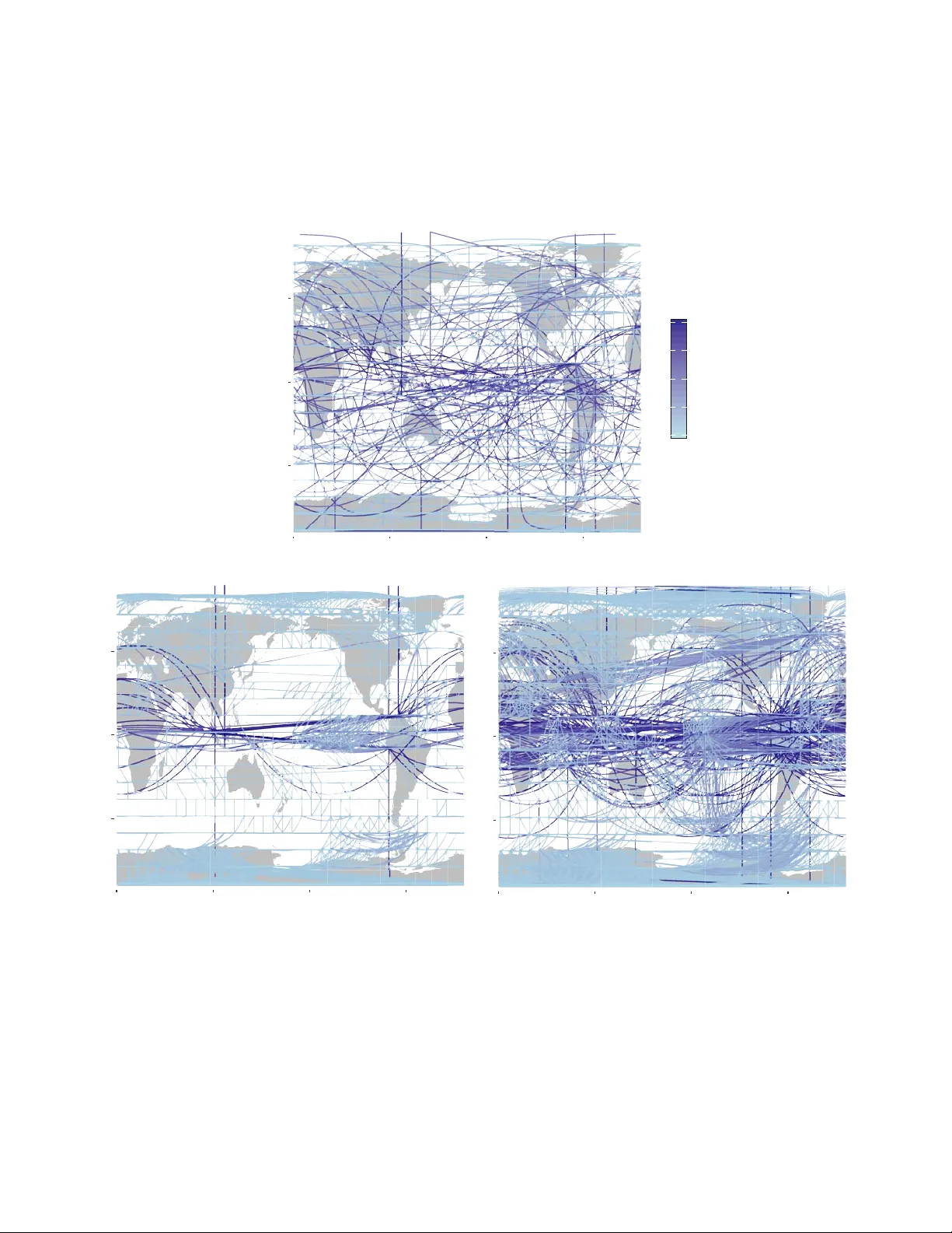
Leave a Comment