A Simple Local Minimal Intensity Prior and An Improved Algorithm for Blind Image Deblurring

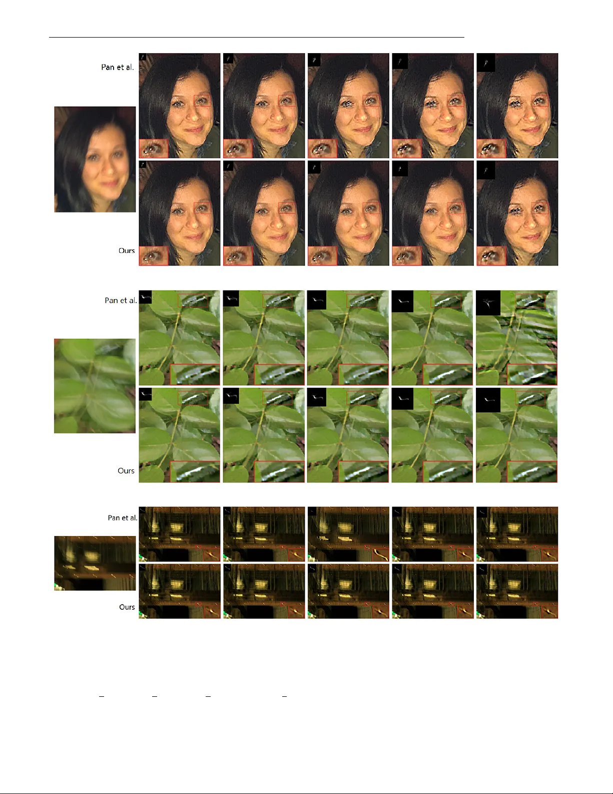
PUBLISHED IN IEEE TRANSA CTIONS ON CIRCUITS AND SYSTEMS FOR VIDEO TECHNOLOGY , DOI:10.1109/TCSVT .2020.3034137 1 A Simple Local Minimal Intensity Prior and An Impro v ed Algorithm for Blind Image Deblurring Fei W en, Rendong Y ing, Y ipeng Liu, Peilin Liu, and T rieu-Kien Truong Abstract —Blind image deblurring is a long standing challeng- ing problem in image pr ocessing and low-level vision. Recently , sophisticated priors such as dark channel prior , extreme channel prior , and local maximum gradient prior , have shown promis- ing effectiveness. However , these methods are computationally expensive. Meanwhile, since these priors inv olved subproblems cannot be solved explicitly , approximate solution is commonly used, which limits the best exploitation of their capability . T o address these problems, this work firstly proposes a simplified sparsity prior of local minimal pixels, namely patch-wise min- imal pixels (PMP). The PMP of clear images is much more sparse than that of blurred ones, and hence is very effective in discriminating between clear and blurr ed images. Then, a novel algorithm is designed to efficiently exploit the sparsity of PMP in deblurring. The new algorithm flexibly imposes sparsity inducing on the PMP under the maximum a posterior (MAP) framework rather than dir ectly uses the half quadratic splitting algorithm. By this, it avoids non-rigorous approximation solution in existing algorithms, while being much more computationally efficient. Extensiv e experiments demonstrate that the proposed algorithm can achieve better practical stability compared with state-of-the-arts. In terms of deblurring quality , robustness and computational efficiency , the new algorithm is superior to state- of-the-arts. Code f or repr oducing the results of the new method is a vailable at https://github.com/FW en/deblur-pmp.git. Index T erms —Image deblurring, blind deblurring, sparsity inducing, local minimal pixels, intensity sparsity prior . I . I N T R O D U C T I O N Blind image deblurring, also known as blind decon volution, aims to recov er a sharp latent image from its blurred obser - vation when the blur kernel is unknown. It is a fundamental problem in image processing and low level vision, which has been extensi vely studied and is still a very activ e research topic in image processing and computer vision. For single image deblurring and under the assumption that the blur is uniform and spatially in variant, the blur process can be modeled as a conv olution operation [1], gi ven by B = k ⊗ I + n, (1) where B , k , I , n , and ⊗ denote the blurred image, blur kernel, latent (clear) image, additiv e noise, and con volution operator , respecti vely . In the blind deblurring problem, only Copyright © 20xx IEEE. Personal use of this material is permitted. Howe ver , permission to use this material for any other purposes must be obtained from the IEEE by sending an email to pubs-permissions@ieee.org. F . W en, R. Ying, P . Liu and T .-K. T ruong are with the Depart- ment of Electronic Engineering, Shanghai Jiao T ong Univ ersity , Shang- hai 200240, China (e-mail: wenfei@sjtu.edu.cn; rdying@sjtu.edu.cn; liu- peilin@sjtu.edu.cn; truong@isu.edu.tw). Y . Liu is with the School of Information and Communication Engineering, Univ ersity of Electronic Science and T echnology of China, Chengdu 611731, China (e-mail: yipengliu@uestc.edu.cn). the blurred image B is known a prior . The objectiv e is to recov er the kernel k and the clear image I simultaneously from B . Basically , it is a highly ill-posed problem as there exist many dif ferent solution pairs of ( k , I ) gi ving rise to the same B . Note that a typical undesired solution is that I = B and k being a delta blur k ernel. T o make the blind deblurring problem well-posed, image prior and blur kernel model exploitation is the key of most effecti ve methods. W ell developed image priors include the gradient sparsity prior [1]–[5], normalized sparsity prior [6], patch prior [7], group sparsity prior [8], intensity prior [9], dark channel prior [10], [11], extreme channel prior [12], latent structure prior [13], local maximum gradient prior [14], class-specific prior [15], and learned image prior using a deep network [16], to name just a few . Meanwhile, blur kernel models include the non-uniform model with blur from multiple homographies [17]–[20], depth variation model [21], [22], in- plane rotation model [23], and forward motion model [24]. Most of these methods exploit image prior and blur k ernel model under the maximum a posterior (MAP) framework. Generally , since the related deblurring problems are non- con vex [25], incorporating regularization to exploit image prior and/or kernel model helps to effecti vely increase the probability of achieving a good local solution. In addition, heuristic edge selection is also an effect way to help the MAP algorithms to a void undesired tri vial solutions. For a more detailed discussion, see [26], [27]. While image gradient sparsity is a popular and commonly used prior , image intensity or gradient based priors hav e sho wn good complementary effecti veness when jointly used with the image gradient prior [9], [10], [12], [14]. As priors and models designed for natural images usually do not generalize well to specific images such as text images [28], face images, and lo w- light images [29], simultaneously exploiting multiple priors has the potential to achiev e satisfactory performance on both natural and specific images [9], [10], [12], [14]. Though the sophisticated priors [10], [12], [14] hav e shown promising ef fecti veness, there e xist two limitations: i) Jointly using multiple priors makes the corresponding algorithms computationally expensi ve. ii) Since these priors in volved subproblems in the corresponding algorithms cannot be solved explicitly , non-rigorous approximate solution is commonly used, which limits the best exploitation of the capability of such priors. These limitations moti vate us to de velop a more effecti ve and efficient method in this work. The main contributions are as follows. PUBLISHED IN IEEE TRANSA CTIONS ON CIRCUITS AND SYSTEMS FOR VIDEO TECHNOLOGY , DOI:10.1109/TCSVT .2020.3034137 2 A. Contribution Firstly , we propose a novel local intensity based prior , namely the patch-wise minimal pix els (PMP) prior . The PMP is a collection of local minimal pixels. Intuitiv ely , since the blur process has a smoothing effect on the image pixels, the intensity of a local minimal pixel would increase after the blur process. As a result, the PMP of clear images are much sparser than those of blurred ones. The PMP metric is as simple as the direct intensity prior , but is very effecti ve in discriminating between clear and blurred images. It can be viewed as a simplification of the dark channel prior in [10], which facilitates efficient computation while being effecti ve. A more detailed comparison with existing intensity priors [9], [10] is pro vided in Section II-B. Secondly , a nov el algorithm is proposed to exploit the sparsity of PMP under the MAP framew ork. The new al- gorithm flexibly imposes sparsity inducing on the PMP of the latent image in the MAP deblurring process. Compared with e xisting algorithms solving augmented MAP formulations directly based on half quadratic splitting, e.g., [10], [12], [14], the proposed algorithm greatly impro ves the computational efficienc y in substance. More importantly , while the algorithms [10], [12], [14] use approximate solution in handling non- explicit subproblems, the ne w algorithm av oids such approxi- mation. As a consequence, in comparison with state-of-the- art methods, it is practically more robust and can achieve competitiv e performance on both natural and specific images. Finally , extensiv e experimental results on blind image de- blurring hav e been provided to ev aluate the performance of the proposed method. The results sho w that the proposed method can achieve state-of-the-art performance on both natural and specific images. In terms of the deblurring quality , rob ustness and computational efficiency , the proposed method is superior to the compared algorithms. B. Related W ork In recent years, single image blind deblurring has made much progress with the aid of various effecti ve priors on images and blur kernels [30]. Most works are based on the variational Bayes and MAP framew orks [1]–[6], [9]–[12], [16], [26], [27], [31]–[36]. T ypically , such a blind deblurring method generally has two steps. First, blur kernel is estimated from the blurred observ ation under the MAP framew ork. Then, based on the estimated blur kernel, the latent sharp image is estimated via non-blind decon volution methods, e.g., [37]– [39]. As the naiv e MAP method could fail on natural images, exploiting the statistical priors of natural images and selection of salient edges are the key of the success of state-of-the-art methods. The gradient sparsity prior of natural images is the most widely used prior . But it has been sho wn in [2] that, in practice, the methods using the gradient sparsity prior in the MAP framework fav or blurry images rather than clear ones. This limitation can be mitigated by techniques as e xp l icit sharp edge pursuit [5], [27], [33], [40] or heuristic edge selection [26]. Howe ver , the assumption of such techniques that there exist strong edges in the latent images may not al ways be satisfied. There also exist various other image priors designed to rein- vigorate MAP , such as normalized sparsity prior [6], internal patch recurrence [32], and direct intensity prior [9]. Though effecti ve for either natural or specific images, such priors usually cannot yield satisfactory performance on both natural and specific images. The recently proposed dark-channel prior [10] and data driv en learned prior [16] can achieve satisfactory performance on both natural and specific images, but the in- volv ed optimization algorithms are computationally expensi ve. Particularly , the intensity based priors considered in [9], [10] are close to our proposed PMP prior . As PMP is computed based on local minimal intensities, it is fundamentally dif ferent from the intensity priors in [9], [10]. A detailed explanation on the difference is provided in Section II-B. Furthermore, our algorithm exploits the PMP sparsity prior in a different way from that in [9], [10] and, as a consequence, it can reduce the computational complexity significantly while has more rob ust (stable) performance. A detailed comparison on the algorithms is provided in Section IV . Recently , data driv en methods hav e also made much success with the aid of powerful deep learning techniques, e.g., [23], [41]–[45]. For example, Sun et al. [23] endeav ored to em- ploy a con volutional neural network (CNN) to estimate and remov e non-uniform motion blur . Nah et al. [42] proposed a multi-scale CNN to recover the latent image in an end- to-end manner without any assumption on the blur kernel. Meanwhile, spatially variant recurrent neural network and scale-recurrent network have been designed for deblurring in [41], [45]. Moreover , Kupyn et al. [44] proposed an end- to-end learned method for deblurring based on conditional generativ e adversarial networks (GAN). In addition, end-to- end CNN model for video deblurring has been considered in [43]. Though these data driv en methods can yield fav or- able performance in various scenarios, their success depends heavily on the consistency between the training data and the test data. This leads to the limitation of their generalization capability . Outline: The rest of this paper is organized as follows. Sec- tion II introduces the sparsity property of PMP and discusses the connection between PMP and existing intensity priors. The new algorithm is dev eloped in detail in Section III. Section IV presents comparison between the proposed algorithm and existing related algorithms. Section V provides e xperimental results. Finally , this paper concludes with a brief summery in Section VI. Notations: ⊗ and ∇ denote the conv olution and gradient operation, respecti vely , d·e denotes the ceil operator , ◦ stands for Hadamard (element-wise) product, ¯ x denotes the conjugate of a complex quantity x . X ( i, j ) denotes the ( i, j ) -th element of a matrix X , F ( X ) denotes the 2-D FFT of X , and F − 1 ( X ) denotes the 2-D inv erse FFT of X . I I . P A T C H - W I S E M I N I M A L P I X E L S This section first introduces the proposed PMP prior and presents analysis on its statistic property . Then, comparison with existing intensity priors is provided. PUBLISHED IN IEEE TRANSA CTIONS ON CIRCUITS AND SYSTEMS FOR VIDEO TECHNOLOGY , DOI:10.1109/TCSVT .2020.3034137 3 Fig. 1. Intensity histogram for patch-wise minimal pixels of clear and blurred images over 5000 natural images (computed with an image patch size of 20 × 20 ). The PMP of clear images (under a threshold such as 0.9) follo ws a hyper Laplacian distribution and is much more sparse than the PMP of blurred images. A. P atch-W ise Minimal Pixels PMP is a collection of local minimal pixels over non- ov erlapping patches. Let an image I ∈ R m × n × c be divided into P non-o verlapped patches with a patch size of r × r , for which P =  m r  ·  n r  . The PMP is defined as P ( I )( i ) = min ( x,y ) ∈ Ω i  min c ∈{ r,g,b } I ( x, y , c )  , (2) for i = 1 , 2 , · · · P , where Ω i denotes the index set of the pixel locations of the i -th patch. It is easy to see that P ( I ) ∈ R P which contains patch-wise (local) minimal pixels of I . In what follows, we show that the PMP of blurred images are much less sparse than those of natural clear images. Fig. 1 compares the histogram statistic of PMP between clear images and their blurred counterparts ov er more than 5000 natural images from the VGG 1 dataset. The blurred images are synthesized from the clear ones using the blur kernels of the dataset [2]. It can be seen from Fig. 1 that the PMP of clear natural images hav e significantly more zero elements than those of blurred images. The PMP of clear images under a threshold (e.g., 0.9) follow a hyper Laplacian distrib ution and manifest a sparsity property . This sparsity property of PMP provides a natural metric to discriminate clear images from blurred ones. Based on this property , the proposed algorithm imposes sparsity inducing on PMP in the deblurring process to achie ve more accurate kernel estimation. Besides the empirical results shown in Fig. 1, the following result theoretically shows that blurred images hav e less sparse PMP than their clear counterparts. Property 1: Let P ( B ) and P ( I ) denote the PMP of the blurred and clear images, respectively . Then P ( B ) ≥ P ( I ) . (3) This property can be directly deriv ed via extending Property 1 in [10]. It indicates that the blur process increases the values 1 http://www .robots.ox.ac.uk/ ∼ vgg/data/ of PMP , which giv es rise to that the PMP of blurred images are less sparse than their clear counterparts. In the following, without loss of generality , consider c = 1 for simplicity . For the PMP P ( I ) : R m × n → R P defined in (2), we further define its in verse operation for later use. Its in verse operation is defined by its transpose P T ( z ) : R P → R m × n for any z ∈ R P . Accordingly , we hav e I p := P T ( P ( I )) = I ◦ M , (4) where M ∈ R m × n is the binary mask corresponding to the PMP subset of I , with M ( i, j ) = 1 if I ( i, j ) is a minimal pixel of a patch and M ( i, j ) = 0 otherwise. B. Comparison with Existing Intensity Sparsity Priors Intensity sparsity has also been considered in [9], [10] for blind deblurring. Howe ver , the proposed PMP is fundamen- tally dif ferent from the intensity metrics considered in [9], [10], which is explained as follo ws. The closest work exploiting intensity sparsity is the dark channel metric considered in [10]. For an image I ∈ R m × n × c , the dark channel is defined as D ( I )( i, j ) = min ( x,y ) ∈ Ω i,j  min c ∈{ r,g,b } I ( x, y , c )  , (5) for i = 1 , 2 , · · · m and j = 1 , 2 , · · · n , where Ω i,j denotes the index set of the pixel locations of the patch centered at the ( i, j ) -th pixel. It is easy to see that D ( I ) ∈ R m × n . While the dark-channel is computed in a con volution like manner with an output of size m × n , the proposed PMP is computed on non-ov erlapped patches with a vector output P ( I ) ∈ R P of size P =  m r  ·  n r  for a patch size of r × r . As a result, the proposed PMP is much simpler than the dark-channel prior, thereby facilitating the design of more ef ficient algorithm. Moreov er , the work [9] uses sparsity inducing directly on the intensity of the image for text image deblurring. Since the intensity distribution of text images is close to two-tone, using ` 0 -regularization to promote the intensity sparsity has demonstrated outstanding ef fectiv eness in text image deblur- ring. Ho wev er , the distrib ution of the intensity values of natural images are more complex than that of text images, and the direct intensity sparsity is not applicable to natural images. In comparison, the proposed PMP metric is as simple as the direct intensity metric [9], but is very effecti ve in discriminating between clear and blurred natural images as shown in Fig. 1. I I I . P R O P O S E D D E B L U R R I N G A L G O R I T H M U S I N G P M P S PA R SI T Y R E G U L A R I Z A T I O N This section presents an efficient algorithm via flexibly incorporating the sparsity regularization of PMP into the con ventional MAP framew ork. The new algorithm is a v ariant of the half quadratic splitting algorithm, but is dif ferent to the direct half quadratic splitting algorithm used in [9], [10], [12], [14], which is explained in detail in Section IV . Recall that the well-known MAP formulation is given by min k,I L ( k ⊗ I , B ) + γ G ( k ) + µR ( I ) , (6) PUBLISHED IN IEEE TRANSA CTIONS ON CIRCUITS AND SYSTEMS FOR VIDEO TECHNOLOGY , DOI:10.1109/TCSVT .2020.3034137 4 where γ and µ are positive weight parameters, and L is a data fidelity term, which restricts k ⊗ I to be consistent with the blurred image B . T o make the problem well-posed, G and R are penalty functions to exploit the structures in the blur kernel and the latent image, respectively . W ith the nature of that the gradient of natural images is sparse, R ( I ) is usually selected as the ` 0 -norm penalty of ∇ I (the gradient of I ). Meanwhile, selecting both the loss function L and the penalty for the kernel as the ` 2 -norm yields min k,I k k ⊗ I − B k 2 2 + γ k k k 2 2 + µ k∇ I k 0 . (7) The ` 2 -norm is not only optimal for Gaussian noise, b ut also enables the dev elopment of ef ficient algorithms because it facilitates fast computation of the in volved subproblems via fast F ourier transform (FFT). T o further exploit the sparsity of the PMP of the latent image, e.g., P ( I ) ∈ R P for a patch size of r × r , now consider a constrained e xtension of (7) as min k,I k k ⊗ I − B k 2 2 + γ k k k 2 2 + µ k∇ I k 0 subject to P ( I )( i ) ∼ p ( x ) , for i ∈ { 1 , · · · , P } . (8) As introduced in Section II, p ( x ) is a probability density func- tion of a hyper Laplacian distribution for x belo w a threshold such as 0.9. The constrained problem (8) is nonsmooth and noncon vex. Similar to most existing deblurring algorithms in solving MAP-like objectiv e functions, we propose an efficient algorithm to solve (8) via alternatingly update the blur kernel and the latent image. In the proposed algorithm, the constraint in (8) is approximately imposed via iteratively sparsity induc- ing on P ( I ) in the latent image subproblem. Note that a natural alternati ve of (8) to promote sparsity of the PMP in the MAP framework is the formulation as follows: min k,I k k ⊗ I − B k 2 2 + γ k k k 2 2 + µ k∇ I k 0 + α kP ( I ) k 0 , (9) where α is a positiv e weight parameter and the last term uses ` 0 -norm penalty to achiev e sparsity inducing on the PMP of the latent image. This formulation can be solved directly by the half quadratic splitting algorithm in an alternating manner similar to the algorithms in [9], [10], [12], [14]. Ho wever , we show that the proposed algorithm for solving (8) is superior to the direct half quadratic splitting algorithm for solving (9), which will be explained in Section IV in detail. A. Estimating the Latent Image Giv en an interim estimation of the blur kernel, denoted by k i , the latent image is updated via optimizing the following problem: min I   k i ⊗ I − B   2 2 + µ k∇ I k 0 subject to P ( I )( i ) ∼ p ( x ) , for i ∈ { 1 , · · · , P } . (10) Using an auxiliary v ariable G with respect to the image gradient ∇ I , the problem (10) can be approximated by min I ,G   k i ⊗ I − B   2 2 + β k∇ I − G k 2 2 + µ k G k 0 subject to P ( I )( i ) ∼ p ( x ) , for i ∈ { 1 , · · · , P } , (11) where β > 0 is a suf ficient large penalty parameter such that it enforces k∇ I − G k 2 2 ≈ 0 , and hence G ≈ ∇ I . W ithout the constraint, such as in the case of the traditional MAP algorithm, the problem (11) can be typically solved using the block coordinate descent algorithm, which alternatingly updates the two variables I and G . The proposed algorithm also solves (11) via alternating between the variables I and G in which the constraint is approximately imposed. Specifically , since the constraint in fact imposes a sparsity regularization on the PMP of I , we use a simple thresh- olding/shrinkage step in the iteration procedure to impose sparsity inducing on the PMP of I . Given I t and at the ( t + 1) -th iteration of the latent image subproblem, denote the PMP subset of I t by I t s := P ( I t ) , we iteratively impose thresholding on I t s and update I and G via the following steps. First, let λ > 0 be a threshold parameter . The PMP is thresholded as ˜ I t +1 ,j s ( i ) =  0 , | I t +1 ,j s ( i ) | < λ I t +1 ,j s ( i ) , otherwise , for i ∈ { 1 , · · · , P } . (12) Subsequently , let Ω t +1 ,j denote the index set of the PMP in I t +1 ,j and define the mask corresponding to the PMP subset to be M t +1 ,j ( i, j ) =  1 , if ( i, j ) ∈ Ω t +1 ,j 0 , otherwise . (13) Then, we update I t +1 ,j as ˜ I t +1 ,j = I t +1 ,j ◦ (1 − M t +1 ,j ) + P T ( ˜ I t +1 ,j s ) , (14) where P T is the inv erse operation of P defined in Section II- A. W ith ˜ I t +1 ,j giv en in (14), the gradient-subproblem solves the follo wing formulation G t +1 ,j +1 = arg min G β    ∇ ˜ I t +1 ,j − G    2 2 + µ k G k 0 , (15) which is a proximal minimization and from [46] the solution is explicitly given by G t +1 ,j +1 ( i, j ) =  0 , ( T ( i, j )) 2 < µ/β T ( i, j ) , otherwise , with T = ∇ ˜ I t +1 ,j . (16) Finally , the latent image is updated via solving the follo wing problem I t +1 ,j +1 = arg min I   k i ⊗ I − B   2 2 + β   ∇ I − G t +1 ,j +1   2 2 , (17) which can be efficiently computed by means of FFT as (18) given in the next page, where ∇ = ( ∇ h , ∇ v ) and G = ( G h , G v ) are used, such that they correspond to image gradients in the horizontal and vertical directions, respectiv ely . This algorithm is summarized in Algorithm 1, which con- tains two loops. In Algorithm 1, a is a positive increasing factor , which is set to a = 2 in the experiments. Extensi ve numerical studies show that the inner loop usually conv erges within a few iterations. For e xample, we use J = 3 in the experiments in Section V . PUBLISHED IN IEEE TRANSA CTIONS ON CIRCUITS AND SYSTEMS FOR VIDEO TECHNOLOGY , DOI:10.1109/TCSVT .2020.3034137 5 I t +1 ,j +1 = F − 1   F ( k i ) ◦ F ( B ) + β  F ( ∇ h ) ◦ F ( G t +1 ,j +1 h ) + F ( ∇ v ) ◦ F ( G t +1 ,j +1 v )  F ( k i ) ◦ F ( k i ) + β  F ( ∇ h ) ◦ F ( ∇ h ) + F ( ∇ v ) ◦ F ( ∇ v )    . (18) Algorithm 1: Latent image estimation Input: Blurred image B , interim kernel estimation k i . β ← β 0 , I 0 ← B . While β ≤ β max do ( t = 0 , 1 , 2 , · · · ) I t +1 , 0 ← I t . For j = 0 : J − 1 do Compute the mask M t +1 ,j via (13) based on I t +1 ,j . Obtain ˜ I t +1 ,j s via (12) and further update ˜ I t +1 ,j via (14). Compute gradient thresholding to obtain G t +1 ,j +1 via (16). Update I t +1 ,j +1 via (18). End for I t +1 ← I t +1 ,J . β ← aβ . End while I i +1 ← I t +1 . Output: Intermediate latent image estimation I i +1 . B. Estimating the Blur Kernel Similar to other existing state-of-the-art algorithms, the kernel estimation is performed in the gradient space. As it has been shown that gradient space based methods are more accurate than intensity space based ones [3], [4], [27]. Specifically , giv en an interim estimation of the latent image, denoted by I i , the blur kernel is updated via solving k i +1 = arg min k   k ⊗ ( ∇ I i ) − ∇ B   2 2 + γ k k k 2 2 . (19) Due to its quadratic form, the solution can be efficiently computed by means of FFT , gi ve by k i +1 = F − 1 F ( ∇ h I i ) ◦ F ( ∇ h B ) + F ( ∇ v I i ) ◦ F ( ∇ v B ) F ( ∇ h I i ) ◦ F ( ∇ h I i ) + F ( ∇ v I i ) ◦ F ( ∇ v I i ) + γ ! . (20) Moreov er , the estimated kernel is further refined via setting the negati ve elements to zero and normalization. In practical implementation, the multi-scale decon volution scheme [27] is adopted to estimate the kernel in a coarse-to-fine manner . The main steps for kernel estimation at a single scale le vel are shown in Algorithm 2. C. Implementation T ricks T o make the augmented objecti ve function in (11) accurately approaching that in (10), a sufficiently lar ge value of β is desired, ideally β → ∞ . Howe ver , with a very large v alue of β , an alternating algorithm directly minimizing (11) would be very slow and impractical. T o address this problem, a standard trick is to use a continuation process for β . In other words, one Algorithm 2: Blind blur kernel estimation Input: Blurred image B , kernel initialization k 0 from the estimation in the last coarser-scale. For i = 1 : max iter do Estimate I i via Algorithm 1 using k i − 1 . Estimate k i via (20). End for ˆ k ← k i , ˆ I ← I i . Output: K ernel estimation ˆ k , intermediate image ˆ I . starts with a properly small v alue of β and gradually increase it by iteration until a large target v alue is reached. This trick is used in Algorithm 1 with a a > 1 . The thresholding step of the PMP in (12) corresponds to a noncon ve x ` 0 -regularization. In addition, the objecti ve function in (11) is also noncon ve x. Hence, with different initialization and/or parameter setting, a noncon vex algorithm would end up with one of its many local minimizers. In view of this, in implementing Algorithm 1, we use soft- thresholding instead of the hard-thresholding in the first few scales in the multi-scale procedure and then turn back to the hard-thresholding. As the soft-thresholding corresponds to the con vex ` 1 -regularization, this “first loose and then tight” strategy makes the proposed algorithm more stable and performing satisfactorily . I V . C O M PA R I S O N W I T H T H E H A L F Q U AD R AT I C S P L I T T I N G A L G O R I T H M S O LV I N G T H E R E G U L A R I Z E D M A P F O R M U L A T I O N ( 9 ) As mentioned in Section III, a natural alternati ve of (8), which can incorporate sparsity inducing of the PMP into the MAP framework, is giv en by (9). Compared with the formulation (8), the formulation (9) is e ven more explicit and can be solved by means of the half quadratic splitting algorithm. Howe ver , in this section we sho w that, compared with the direct half quadratic splitting algorithm solving (9), the proposed algorithm is not only superior in computational complexity , but also can avoid non-rigorous approximate so- lution in solving the regularized MAP problem. T o solve (9) with a giv en interim kernel estimation k i , the latent image problem becomes min I   k i ⊗ I − B   2 2 + µ k∇ I k 0 + α kP ( I ) k 0 . (21) Similar to [13], [14], using two auxiliary v ariables G and Z with respect to ∇ I and P ( I ) , respectively , the problem (21) is approximated by min I   k i ⊗ I − B   2 2 + µ k G k 0 + α k Z k 0 + β k∇ I − G k 2 2 + ρ kP ( I ) − Z k 2 2 , (22) PUBLISHED IN IEEE TRANSA CTIONS ON CIRCUITS AND SYSTEMS FOR VIDEO TECHNOLOGY , DOI:10.1109/TCSVT .2020.3034137 6 Algorithm 3: Latent image estimation via solving (22) Input: Blurred image B , interim kernel estimation k i . ρ ← ρ 0 , I 0 ← B . While ρ ≤ ρ max do ( t = 0 , 1 , 2 , · · · ) Compute Z t +1 via (23) using I t . β ← β 0 , I t +1 , 0 ← I t . While β ≤ β max do ( j = 0 , 1 , 2 , · · · ) Obtain G t +1 ,j +1 via (24) using I t +1 ,j . Solve (25) to update I t +1 ,j +1 . β ← aβ . End while I t +1 ← I t +1 ,J . ρ ← aρ . End while I i +1 ← I t +1 . Output: Intermediate latent image estimation I i +1 . where β and ρ are positiv e penalty parameters. Given I t at the ( t + 1) -th iteration, the G - and Z -subproblems are proximity operators, which can be efficiently solved in an element-wise manner as Z t +1 ( i, j ) =  0 , ( Y ( i, j )) 2 < α/ρ Y ( i, j ) , otherwise , with Y = P ( I t ) , (23) and G t +1 ( i, j ) =  0 , ( T ( i, j )) 2 < µ/β T ( i, j ) , otherwise , with T = ∇ I t . (24) Then, the I -subproblem becomes min I   k i ⊗ I − B   2 2 + β   ∇ I − G t +1   2 2 + ρ   P ( I ) − Z t +1   2 2 . (25) In view of that there exist tw o augmentation terms in the noncon vex problem (22), to mak e the algorithm practically working well, a standard trick is to use a continuation process for each of β and ρ similar to the algorithms in [9], [10]. In such a manner , the main steps of the half quadratic splitting algorithm are sk etched in Algorithm 3. Although both Algorithms 1 and 3 contain two main loops, the former is much more efficient than the latter in practice. That is because the penalty parameters ρ max and β max in Algorithm 3 should be chosen sufficiently lar ge to make (22) accurately approximating for (21), while a small value of J (e.g., J = 3 ) is enough for Algorithm 1 to giv e satisfactory performance. Moreov er , although the I -step in Algorithm 3 solves a quadratic problem (25), it cannot be efficiently solved via FFT similar to (18). A strategy to e xplicitly solve the least-square problem (25) in closed-form is to vectorize the variables and con vert the con volution operation into linear multiplication. Howe ver , this least-square problem in volves computing the in verse of high-dimensional matrices of size ( mn ) × ( mn ) with m × n be the size of I . Thus, it is computationally expensi ve to handle practical-sized inputs. Meanwhile, since P ( I ) is a subsampling function of I and only contains a subset of the pix els of I , clearly , the problem (25) cannot be solved in closed-form via FFT similar to (18) and the algorithms as giv en in [6], [32], [47]. W ith the definition in (4), problem (25) can be equiv alently rewritten as min I   k i ⊗ I − B   2 2 + β   ∇ I − G t +1   2 2 + ρ   I p − P T ( Z t +1 )   2 2 . (26) Now , let ˘ I p = I ◦ (1 − M ) be the complementary set of I p such that it satisfies I p + ˘ I p = I . It is easy to see from (25) that I p and ˘ I p are coupled through the kernel con volution operation. W ith this in mind, to enable FFT based ef ficient solution, we can iterati vely solve (26) via alternating between I p and ˘ I p . For e xample, we first fix ˘ I p to solve I p by min I p    k i ⊗ I p − ( B − k i ⊗ ˘ I p )    2 2 + β    ∇ I p − ( G t +1 − ∇ ˘ I p )    2 2 + ρ   I p − P T ( Z t +1 )   2 2 , (27) and then fix I p to solve ˘ I p by min ˘ I p    k i ⊗ ˘ I p − ( B − k i ⊗ I p )    2 2 + β    ∇ ˘ I p − ( G t +1 − ∇ I p )    2 2 . (28) Thanks to the quadratic form of (26), iterativ ely solving (27) and (28) is guaranteed to con verge to the global minimizer of (26) with any bounded initialization. Even though both (27) and (28) can be efficiently solved by means of FFT , iteratively solving them mak es Algorithm 3 having three iteration loops, and hence results in an increase of computational complexity in terms of runtime. Note that in the dark-channel based method [10], the I - subproblem has a similar formulation as (25), where P ( I ) is replaced by the dark-channel e xtraction operation, which is solved via FFT in close-form. The close-form solution is deriv ed via implicitly using an approximation. That is kD I t ( I ) − u k 2 2 ≈    I −  D T I t ( u ) + ˘ I t d     2 2 , (29) where D I t denotes the dark-channel extraction operator based on I t , D T I t is the inv erse operator of D I t , and ˘ I t d is the complementary set of I t d with I t d being the subset pixels of I t which forms the dark-channel. In fact, the right term in (29) can be viewed as an approximation of   D T I t ( D I t ( I )) − D T I t ( u )   2 2 =   I d − D T I t ( u )   2 2 =    I −  D T I t ( u ) + ˘ I d     2 2 , (30) where D T I t ( D I t ( I )) = I d and I = I d + ˘ I d are used. Similar approximation has also been used in [12], [14]. In comparison, the proposed Algorithm 1 completely av oids such approximation and would be more stable in practical applications, as demonstrated by the results in Fig. 2, 3 and T able II in the e xperiments. PUBLISHED IN IEEE TRANSA CTIONS ON CIRCUITS AND SYSTEMS FOR VIDEO TECHNOLOGY , DOI:10.1109/TCSVT .2020.3034137 7 T ABLE I Q UA N TI TA T I V E E V A L UA T I O N O F T H E N E W M E T HO D V E R SU S PA T C H S I Z E O N T H E DAT A S ET [ 5 0 ] ( A V E R AG E P S N R A N D S S I M ). Patch size PSNR (dB) SSIM 0 . 015 · mean ( m, n ) 29.5891 0.8754 0 . 020 · mean ( m, n ) 29.6397 0.8778 0 . 025 · mean ( m, n ) 29.9764 0.8944 0 . 030 · mean ( m, n ) 29.7355 0.8837 0 . 035 · mean ( m, n ) 29.7088 0.8822 V . E X P E R I M E N TA L R E S U LT S W e firstly in vestigate the robustness of the new algo- rithm in terms of sensitivity against the kernel size pa- rameter , in comparison with the most close method [10]. Then, we ev aluate the proposed algorithm on three bench- mark datasets in comparison with state-of-the-art blind image deblurring methods. Furthermore, we conduct e valuation on face, natural, text, and low-light images. Matlab code for reproducing the results of the ne w algorithm is a vailable at https://github .com/FW en/deblur-pmp.git . For the new algorithm, µ = 4 × 10 − 3 , a = 2 , J = 3 , β 0 = 2 µ , and β max = 10 5 are used. For each scale, we use max iter = 5 as a trade-off between accuracy and speed. The threshold parameter for PMP is initially set to λ = 0 . 1 and gradually reduced to the mean of the PMP values. Note that, in general the optimal values of these parameters depend on the distrib ution of the clear images, the kernel models, the optimization algorithm used for the non-con ve x deblurring problem. Hence, it is difficult to select the optimal values of these parameters. Like most blind deblurring methods, such as the ones compared in the sequel, these parameters are selected empirically in practice. The “first loose and then tight” strategy introduced in Section III-C is employed to make the algorithm performing practically well. The patch size is set dependent on the image size as r = 0 . 025 · mean ( m, n ) . Similar to [2], [5], [10], [26], we first estimate the blur kernel by the proposed algorithm, and then obtain the final latent image based on the estimated kernel by a non-blind deblurring method. The non-blind deblurring algorithm [9] is employed for the final latent image estimation. The performance of the compared algorithms is ev aluated in terms of peak-signal-to-noise ratio (PSNR), structural similarity (SSIM) [48] and cumulativ e error ratio of the deblurred images and kernel estimation. T able I presents a quantitati ve e v aluation of the proposed method versus the patch size r on the dataset [50]. It can be seen that the new method is robust to the patch size. A. Robustness: Sensitivity to the K ernel Size P arameter As discussed in Section IV , the new algorithm can av oid the non-rigorous approximation in solving non-explicit priors (e.g., dark-channel) in volv ed subproblems in [10], [12], [14]. This brings the new algorithm a potential advantage of being more stable in practical applications. T o illustrate this point, the first experiment compares the performance of the new algorithm with Pan et al. [10] through in vestigating their sensitivity ag ainst the kernel size parameter . The selection of T ABLE II A V E RA GE P S N R A N D S S I M O N D E BL U R R IN G 1 2 S A M PL E S O F T H E DAT A S E T [ 5 0 ] A S S O CI A T E D W I TH T H E K E R NE L S 8 , 9 A N D 1 0 . Kernel size 111 121 131 141 151 Pan et al. (PSNR) 22.40 22.85 21.71 23.13 21.69 Ours (PSNR) 23.05 23.35 23.42 23.39 22.49 Pan et al. (SSIM) 0.7503 0.7651 0.7087 0.7612 0.7141 Ours (SSIM) 0.7540 0.7708 0.7806 0.7619 0.7148 (a) PSNR (b) SSIM Fig. 2. PSNR and SSIM versus kernel size on deblurring 12 samples of the dataset [50] associated with the kernels 8, 9 and 10. the kernel size parameter has a substantial influence on the performance of most deblurring algorithms. T able II and Fig. 2 present the PSNR and SSIM results of the two compared methods versus kernel size on deblurring three challenging kernels in the dataset [50] (the kernels 8, 9 and 10). These selected kernels are the most challenging kernels in the dataset [50], which have sizes of more than 100 pixels. There are four samples for each of the three kernels. Moreov er , Fig. 3 shows deblurred results of the two algorithms when using different values of the kernel size parameter on three realistic images. It can be seen from Fig. 2, 3, and T able II that our method is less sensitiv e to the kernel size variation, which demonstrates its better robustness in practice. B. Evaluation on Benc hmark Datasets The second experiment uses the dataset by Kohler et al. [50], which contains 48 blurred samples corresponding to 4 clear images and 12 blur kernels. The compared algorithms include Cho and Lee [27], Xu and Jia [26], Shan et al. [31], Fergus et al. [5], Krishnan et al. [6], Whyte et al. [47], Hirsch et al. [49], and Pan et al. [10]. Fig. 4 presents a statistical analysis of the PSNR and SSIM results of the compared algorithms on deblurring the 48 blurred images. T able III shows the av erage PSNR and average SSIM of the algorithms. The PSNR and SSIM of each deblurred image are computed via comparing it with 199 clear images captured within the camera motion trajectory . The results of the methods [5], [6], [26], [27], [31], [47], [49] are those reported in [50], while the result of the method [10] is computed from the deblurred results provided by the authors at their website 2 . It can be seen that the ne w algorithm can achieve state- of-the-art performance in terms of the PSNR and SSIM results. Fig. 5 presents visual comparison on four challenging 2 http://vllab1.ucmerced.edu/ ∼ jinshan/projects/dark-channel-deblur/ PUBLISHED IN IEEE TRANSA CTIONS ON CIRCUITS AND SYSTEMS FOR VIDEO TECHNOLOGY , DOI:10.1109/TCSVT .2020.3034137 8 (a) The first image. From left to right, the used kernel sizes are { 25, 35, 45, 55, 65 } . (b) The second image. From left to right, the used kernel sizes are { 45, 55, 65, 75, 85 } . (c) The third image. From left to right, the used kernel sizes are { 65, 75, 85, 95, 105 } . Fig. 3. Comparison between Pan et al. [10] and ours method on the three blurred images. For each method, different kernel sizes are tested. images with heavy blurs from the dataset [50], including the ‘Blurry1 8’, ‘Blurry2 9’, ‘Blurry3 10’, and ‘Blurry4 11’ images. It can be inferred from Fig. 5 that the proposed algorithm can achieve comparable or e ven better visual results compared with e xisting state-of-the-art methods [3], [10]. Fig. 6 further in vestigates the effecti veness of the proposed PMP regularization to show the results of the new algorithm with and without PMP regularization on the benchmark dataset [50]. The results demonstrate that the PMP regularization giv es rise to distinct PSNR and SSIM improv ement. The third experiment uses the dataset by Le vin et al. [2], which contains 32 blurred samples corresponding to 4 clear PUBLISHED IN IEEE TRANSA CTIONS ON CIRCUITS AND SYSTEMS FOR VIDEO TECHNOLOGY , DOI:10.1109/TCSVT .2020.3034137 9 (a) PSNR (b) SSIM Fig. 4. Quantitativ e evaluation results on the benchmark dataset of Kohler et al. [50] (PSNR and SSIM comparison over 48 blurry images). T ABLE III Q UA N TI TA T I V E R E SU LT S O N T H E DAT A S ET O F K O HL E R et al. [ 5 0 ] , I N CL U D I NG T H E A V E R AG E P S N R A N D AVE R AG E S S I M . Method PSNR (dB) SSIM Cho and Lee 28.9831 0.8746 Xu and Jia 29.5373 0.8851 Shan et al. 25.8912 0.7748 Fergus et al. 22.7303 0.7048 Krishnan et al. 25.7246 0.7608 Whyte et al. 27.8441 0.8116 Hirsch et al. 26.8388 0.8095 Pan et al. 29.9513 0.8853 Ours 29.9764 0.8944 T ABLE IV Q UA N TI TA T I V E R E SU LT S O N T H E DAT A S ET O F L E V I N et al. [ 2 ] , I N CL U D I NG T H E A V E R AG E P S N R A N D AVE R AG E S S I M . Method PSNR (dB) SSIM Levin et al. 31.1372 0.8960 Fergus et al. 29.4629 0.8451 Cho and Lee 30.7927 0.8837 Xu and Jia 31.3604 0.9083 Pan et al. 31.7297 0.9148 Ours 32.4450 0.9344 images and 8 blur k ernels. The parameter µ is set to 5 × 10 − 3 for all examples. Fig. 7 shows the cumulativ e error ratios of the compared algorithms, which are computed based on the sum of square difference (SSD) error as follo ws. Firstly , for a restored image, the SSD error is computed as the SSD between it and its clear counterpart using the best shift between them. Then, this SSD error is normalized with respect to the SSD error of the de-conv olution result using the ground-truth kernel, which results in an error ratio. Finally , from the error ratios of all the deblurred images, the cumulati ve error ratio is computed to get the success rate. It is empirically noticed that deblurred results with error ratios abov e 2 are visually implausible. T able IV compares the av erage PSNR and a verage SSIM of the methods, whilst Fig. 8 presents statistical analysis of the PSNR and SSIM results It can be observed from T able IV , Fig. 7 and Fig. 8 that, the proposed algorithm achie ves the best PSNR and SSIM results while attaining 100% success at an error ratio of 2 on the dataset [2]. Fig. 9 illustrates the estimated kernels by the proposed algorithm on this dataset, whilst Fig. 10 presents the deblurred results of the proposed algorithm on T ABLE V Q UA N TI TA T I V E R E SU LT S O N T H E DAT A S ET [ 7 ] , I N C L UD I N G T H E A V E R AG E P S NR A N D A V ER A GE S S I M. Method PSNR (dB) SSIM Cho and Lee 26.7548 0.8224 Cho et al. 17.9599 0.4922 Krishnan et al. 23.4366 0.7571 Levin et al. 25.4989 0.8079 Xu and Jia 29.1466 0.8553 Pan et al. 30.2502 0.8587 Ours 30.5660 0.8593 four challenging samples in this dataset. The fourth experiment further considers a much larger dataset of Sun et al. [7], which contains 640 blurred samples corresponding to 80 clear images and 8 blur kernels. Fig. 11 shows the cumulative error ratios of the algorithms on this dataset. The compared algorithms include Cho and Lee [27], Cho et al. [33], Krishnan et al. [6], Levin et al. [2], Xu and Jia [26], and Pan et al. [10]. T able V compares the av erage PSNR and av erage SSIM of the algorithms, whilst Fig. 12 presents statistical analysis of the PSNR and SSIM results. It can be seen that the proposed algorithm can achieve the state-of-the- art performance in terms of cumulativ e error ratio, PSNR and SSIM of re vcovery . C. Evaluation on Natur al and Specific Images In what follows, the proposed method is further ev al- uated on face, natural, text, and low-light images. Here we only provide some typical results for each class due to limited space. More samples are provided online at https://github .com/FW en/deblur-pmp.git . Face image: Face image deblurring is challenging for methods developed for natural images, since the lack of edges and textures in face images makes accurate kernel estimation challenging. Fig. 13 compares the proposed method with the methods [3], [10] on two realistic blurred face images. The results demonstrate that our method compares fa vorably or ev en better against the methods give in [3], [10]. Natural image: The results of the compared algorithms on two real natural images are shown in Fig. 14. Again, our algorithm compares competitiv ely against the methods [3], [10]. It can be see that the proposed PMP regularization helps to significantly reduce the ringing artifacts in the deblurred image, which makes the proposed algorithm yielding state-of- the-art performance. T ext image: The results of the compared algorithms on two text images are illustrated in Fig. 15. Our algorithm performs comparably with the method [10]. When without using the PMP re gularization, our algorithm may fail to reconstruct the correct blur kernel and yields a result with heavy ringing artifacts. Low-light image: Low-light images usually cannot be well handled by most deblurring methods. A main reason is that low-light images often hav e saturated pixels which interfere with the kernel estimation process [29], [51]. Fig. 16 presents the results on a lo w-light image. The state-of-the-art lo w- light image deblurring method [29] is used in the comparison. PUBLISHED IN IEEE TRANSA CTIONS ON CIRCUITS AND SYSTEMS FOR VIDEO TECHNOLOGY , DOI:10.1109/TCSVT .2020.3034137 10 (a) Blurred image (b) Xu et al. [3] (c) Pan et al. [10] (d) Ours Fig. 5. V isual comparison on four challenging images from the dataset [50]. From top to bottom are, respectiv ely , the ‘Blurry1 8’, ‘Blurry2 9’, ‘Blurry3 10’, and ‘Blurry4 11’ images. (a) (b) (c) (d) Fig. 6. Quantitati ve results of the proposed algorithm with or without PMP regularization on the dataset [50]. (a), (b): PSNR and SSIM o ver 12 blurry samples of each of the 4 images. (c), (d): PSNR and SSIM o ver all the 48 blurry samples. Compared with the method [29] specifically designed for lo w- light images, our method gives a comparable result. D. Computational Comple xity Finally , we compare the computational comple xity of our al- gorithm ( r = 0 . 025 · mean ( m, n ) ) with those of the algorithms [3], [4], [10]. Our algorithm without PMP and our algorithm with different patch size r ∈ { 4 , 8 , 16 } are also compared. As explained in Section IV , the proposed Algorithm 1 w ould be more ef ficient than the traditional half quadratic splitting (HQS) algorithm, e.g. Algorithm 3. T o substantiate this, the runtime of the HQS algorithm using the PMP (Algorithm 3) is also compared (with r = 0 . 025 · mean ( m, n ) ). The simulations are conducted under W indows 10 on a desktop PC with an Intel Core i7-4790 CPU at 3.6 GHz with 16 GB RAM. For our method and the methods [4], [10], the runtime of the non-blind deblurring step is included in the results. Among these algorithms, one can observe from T able VI that the PUBLISHED IN IEEE TRANSA CTIONS ON CIRCUITS AND SYSTEMS FOR VIDEO TECHNOLOGY , DOI:10.1109/TCSVT .2020.3034137 11 Fig. 7. Cumulative error ratios of the compared algorithms on the dataset of Levin et al. [2]. (a) PSNR (b) SSIM Fig. 8. Quantitativ e evaluation results on the benchmark dataset of Levin et al. [2] (PSNR and SSIM comparison over 32 blurry images). Fig. 9. Estimated kernels by the proposed algorithm on the dataset [2]. algorithm dev eloped by Xu et al. [3] with C++ implementation is the fastest. Howe ver , in some cases, its restoration quality is inferior to our algorithm as illustrated earlier in the above figures. Our algorithm is much faster than the algorithms [4], [10]. Compared with the algorithm of Pan et al. [10], our algorithm is more than an order of magnitude faster . Note that, the algorithm [10] can be accelerated in the dark-channel computation step as mentioned by the authors. The result of this algorithm presented here is obtained by the code provided by the authors at their website, which is implemented without such acceleration. V I . C O N C L U S I O N This work proposed a local minimal intensity based prior , namely PMP , and an improved algorithm for blind image deblurring. The prior is simple yet effecti ve in discriminating between clear and blurred images. Rather than directly using (a) im01 ker04 (b) im01 ker06 (c) im01 ker07 (d) im01 ker08 Fig. 10. Deblurred results by the proposed algorithm on four challenging samples in the dataset [2]. Fig. 11. Cumulative error ratios of the compared algorithms on the dataset [7]. (a) PSNR (b) SSIM Fig. 12. Quantitative ev aluation results on the benchmark dataset [7] (PSNR and SSIM comparison over 640 blurry images). the half quadratic splitting algorithm, the ne w algorithm fle x- ibly imposes sparsity inducing on the PMP in the deblurring procedure under the MAP framew ork. Particularly , it avoids non-rigorous approximate solution in existing algorithms in PUBLISHED IN IEEE TRANSA CTIONS ON CIRCUITS AND SYSTEMS FOR VIDEO TECHNOLOGY , DOI:10.1109/TCSVT .2020.3034137 12 (a) Blurred image (b) Xu et al. [3] (c) Pan et al. [10] (d) Ours without PMP (e) Ours Fig. 13. V isual comparison on two realistic blurred face images. (a) Blurred image (b) Xu et al. [3] (c) Pan et al. [10] (d) Ours without PMP (e) Ours Fig. 14. V isual comparison on two real natural images. jointly handling multiple non-explicit priors, while being much more efficient. Extensiv e experiments on both natural and specific images demonstrated that it not only can achie ve state- of-the-art deblurring quality , but also can improv e the practical stability and computational efficienc y substantially . In brief, in terms of both the practical robustness and computational efficienc y , the proposed algorithm is superior to the compared algorithms in this work. R E F E R E N C E S [1] T . F . Chan and C.-K. W ong, “T otal variation blind deconv olution, ” IEEE T rans. Image Process. , vol. 7, no. 3, pp. 370–375, Mar . 1998. [2] A. Levin, Y . W eiss, F . Durand, and W . T . Freeman, “Understanding and ev aluating blind deconv olution algorithms, ” in Proc. IEEE Conf. Comput. V is. P attern Recognit. , 2009, pp. 1964–1971. [3] L. Xu, S. Zheng, and J. Jia, “Unnatural L0 sparse representation for natural image deblurring, ” in Pr oc. IEEE Conf. Comput. V is. P attern Recognit. , 2013, pp. 1107–1114. [4] A. Levin, Y . W eiss, F . Durand, and W . T . Freeman, “Efficient marginal likelihood optimization in blind decon volution, ” in Pr oc. IEEE Conf. Comput. V is. P attern Recognit. , 2011, pp. 2657–2664. [5] R. Fergus, B. Singh, A. Hertzmann, S. T . Roweis, and W . T . Freeman, “Removing camera shake from a single photograph, ” ACM SIGGRAPH , vol. 25, no. 3, pp. 787–794, 2006. [6] D. Krishnan, T . T ay , and R. Fergus, “Blind decon volution using a normalized sparsity measure, ” in Proc. IEEE Conf. Comput. V is. P attern Recognit. , 2011. PUBLISHED IN IEEE TRANSA CTIONS ON CIRCUITS AND SYSTEMS FOR VIDEO TECHNOLOGY , DOI:10.1109/TCSVT .2020.3034137 13 (a) Blurred image (b) Xu et al. [3] (c) Pan et al. [10] (d) Ours without PMP (e) Ours Fig. 15. V isual comparison on two text images deblurring. (a) Blurred image (b) Hu et al. [29] (c) Pan et al. [10] (d) Ours without PMP (e) Ours Fig. 16. V isual comparison on a low-light image. T ABLE VI R U N T IM E C O MPA R IS O N I N S E CO N D S ( T H E K E RN E L S I Z E I S FI X E D A T 51 × 51 F O R E A CH A L G OR I T H M ) . Method 256 × 256 512 × 512 800 × 800 Xu et al. (C++) 1.05 2.43 5.35 Levin et al. (Matlab) 155.9 657.8 1598.6 Pan et al. (Matlab) 162.5 548.6 1261.3 HQS (Alg. 3) (Matlab) 107.3 401.2 938.8 Ours w/o PMP (Matlab) 5.59 14.51 35.03 Ours ( r = 4 ) (Matlab) 38.88 132.7 295.3 Ours ( r = 8 ) (Matlab) 16.39 55.73 134.8 Ours ( r = 16 ) (Matlab) 11.02 41.69 94.74 Ours ( r = 0 . 025 m ) (Matlab) 18.61 44.36 95.55 [7] L. Sun, S. Cho, J. W ang, and J. Hays, “Edge-based blur kernel estimation using patch priors, ” in Proc. IEEE Int. Conf. Comput. Photography , 2013, pp. 1–8. [8] T . C. Lin, L. Hou, H. Liu, Y . Li, and T . K. T ruong, “Reconstruction of single image from multiple blurry measured images, ” IEEE T rans. Image Pr ocessing , vol. 27, no. 6, pp. 2762–2776, 2018. [9] J. Pan, Z. Hu, Z. Su, and M.-H. Y ang, “Deblurring text images via L0- regularized intensity and gradient prior, ” in Pr oc. IEEE Conf . Comput. V is. P attern Recognit. , 2014, pp. 2901–2908. [10] J. Pan, D. Sun, H. Pfister , and M.-H. Y ang, “Blind image deblurring using dark channel prior, ” in Pr oc. IEEE Conf. Comput. V is. P attern Recognit. , 2016, pp. 1628–1636. [11] J. Pan, D. Sun, H. Pfister , and M. H. Y ang, “Deblurring images via dark channel prior , ” IEEE T rans. P attern Analysis and Machine Intelligence , vol. 40, no. 10, pp. 2315–2328, 2018. [12] Y . Y an, W . Ren, Y . Guo, R. W ang, and X. Cao, “Image deblurring via extreme channels prior , ” in Proc. IEEE Conf. Comp. V is. P att. Recogn. , 2017, pp. 6978–6986. [13] Y . Bai, H. Jia, M. Jiang, X. Liu, X. Xie, and W . Gao, “Single image blind deblurring using multi-scale latent structure prior, ” IEEE T rans. Cir cuits and Systems for V ideo T echnology , vol. 30, no. 7, pp. 2033–2045, 2019. [14] L. Chen, F . Fang, T . W ang, and G. Zhang, “Blind image deblurring with local maximum gradient prior, ” in Pr oc. IEEE Conf. Comput. V is. P attern Recognit. (CVPR) , 2019, pp. 1742–1750. [15] S. Anwar , C. P . Huynh, and F . Porikli, “Image deblurring with a class- specific prior, ” IEEE T rans. P attern Analysis and Machine Intelligence , vol. 41, pp. 2112–2130, 2018. [16] L. Li, J. Pan, W .-S. Lai, C. Gao, N. Sang, and M.-H. Y ang, “Learning a discriminativ e prior for blind image deblurring, ” in Proc. IEEE Conf. Comp. V is. P att. Recogn. , 2018, pp. 6616–6625. [17] Z. Hu, L. Xu, and M.-H. Y ang, “Joint depth estimation and camera shak e remov al from single blurry image, ” in Proc. IEEE Conf. Comp. V is. P att. Recogn. , 2014, pp. 2893–2900. [18] A. Gupta, N. Joshi, C. L. Zitnick, M. Cohen, and B. Curless, “Single image deblurring using motion density functions, ” in Proc. Eur opean Conf. Computer V ision , 2010, pp. 171–184. [19] O. Whyte, J. Si vic, A. Zisserman, and J. Ponce, “Non-uniform deblurring for shaken images, ” Int. J. Comput. V is. , vol. 98, no. 2, pp. 168–186, 2012. [20] L. Zhang, L. Zhou, and H. Huang, “Bundled kernels for nonuniform blind video deblurring, ” IEEE T rans. Circuits and Systems for V ideo T echnology , vol. 27, no. 9, pp. 1882–1894, 2016. [21] L. Xu and J. Jia “Depth-aware motion deblurring, ” in Pr oc. IEEE Int. Conf. Computational Photography , 2012, pp. 1–8. [22] B. Sheng, P . Li, X. Fang, P . T an, and E. Wu, “Depth-aware motion deblurring using loopy belief propagation, ” IEEE T rans. Cir cuits and Systems for V ideo T echnology , vol. 30, no. 4, pp. 955–969, 2020. [23] J. Sun, W . Cao, Z. Xu, and J. Ponce, “Learning a conv olutional neural network for non-uniform motion blur removal, ” in Pr oc. IEEE Conf. Comp. V is. P att. Recogn. , 2015, pp. 769–777. PUBLISHED IN IEEE TRANSA CTIONS ON CIRCUITS AND SYSTEMS FOR VIDEO TECHNOLOGY , DOI:10.1109/TCSVT .2020.3034137 14 [24] S. Zheng, L. Xu, and J. Jia, “Forward motion deblurring, ” in Proc. IEEE Int. Conf. Comp. V is. , 2013. [25] F . W en, R. Y ing, P . Liu, and R. C. Qiu, “Robust PCA Using Generalized Noncon ve x Regularization, ” IEEE T rans. Cir cuits and Systems for V ideo T echnology , vol. 30, no. 6, 2019. [26] L. Xu and J. Jia, “T wo-phase kernel estimation for robust motion deblurring, ” in Pr oc. Eur . Conf. Comput. V is. , 2010, pp. 157–170. [27] S. Cho and S. Lee, “Fast motion deblurring, ” in Pr oc. ACM SIGGRAPH Asia , vol. 28, no. 5, 2009, Art. no. 145. [28] H. Cho, J. W ang, and S. Lee, “T ext image deblurring using text-specific properties, ” in Pr oc. European Conf. Computer V ision (ECCV) , 2012, pp. 524–537. [29] Z. Hu, S. Cho, J. W ang, and M.-H. Y ang, “Deblurring low-light images with light streaks, ” in Pr oc. IEEE Conf. Comput. V is. P attern Recognit. , 2014, pp. 3382–3389. [30] J. Jia. Mathematical models and practical solvers for uniform motion deblurring . Cambridge Univ ersity Press, 2014. [31] Q. Shan, J. Jia, and A. Agarwala, “High-quality motion deblurring from a single image, ” ACM SIGGRAPH , vol. 27, no. 3, 2008, Art. no. 73. [32] T . Michaeli and M. Irani, “Blind deblurring using internal patch recur- rence, ” in Pr oc. Eur . Conf. Comput. V is. , 2014, pp. 783–798. [33] T . S. Cho, S. P aris, B. K. P . Horn, and W . T . Freeman, “Blur kernel estimation using the radon transform, ” in Proc. IEEE Conf. Comp. V is. P att. Recogn. , 2011, pp. 241–248. [34] D. Wipf and H. Zhang, “Revisiting Bayesian blind deconv olution, ” J . Mach. Learn. Res. , vol. 15, no. 1, pp. 3595–3634, Jan. 2014. [35] G. Liu, S. Chang, and Y . Ma, “Blind image deblurring using spectral properties of con volution operators, ” IEEE T rans. Ima ge Pr ocess. , vol. 23, no. 12, pp. 5047–5056, Dec. 2014. [36] D. Perrone and P . Fa varo, “T otal variation blind deconv olution: The devil is in the details, ” in Pr oc. IEEE Conf. Comput. V is. P attern Recognit. (CVPR) , Jun. 2014, pp. 2909–2916. [37] J. Zhang, D. Zhao, R. Xiong, S. Ma, and W . Gao, “Image restoration using joint statistical modeling in a space-transform domain, ” IEEE T rans. Cir cuits and Systems for V ideo T echnology , vol. 24, no. 6, pp. 915–928, 2014. [38] D. Krishnan and R. Fergus, “Fast image decon volution using hyperlapla- cian priors, ” in Pr oc. Adv . Neural Inf. Process. Syst. (NIPS) , 2009, pp. 1033–1041. [39] D. Zoran and Y . W eiss, “From learning models of natural image patches to whole image restoration, ” in Pr oc. IEEE Int. Conf. Comput. V is. (ICCV) , Nov . 2011, pp. 479–486. [40] J. H. Money and S. H. Kang, “T otal variation minimizing blind decon- volution with shock filter reference, ” Image and V ision Computing , vol. 26, no. 2, pp. 302–314, 2008. [41] J. Zhang, J. Pan, J. Ren, Y . Song, L. Bao, R. W . Lau, and M.-H. Y ang, “Dynamic scene deblurring using spatially variant recurrent neural networks, ” in Pr oc. IEEE Conf. Comp. V is. P att. Recogn. , 2018. [42] S. Nah, T . H. Kim, and K. M. Lee, “Deep multiscale con volutional neural network for dynamic scene deblurring, ” in Proc. IEEE Conf. Comp. V is. P att. Recogn. , July 2017. [43] S. Su, M. Delbracio, J. W ang, G. Sapiro, W . Heidrich, and O. W ang, “Deep video deblurring for handheld cameras, ” in Pr oc. IEEE Conf. Comp. V is. P att. Recogn. , July 2017. [44] O. Kupyn, V . Budzan, M. Mykhailych, D. Mishkin, and J. Matas, “De- blurgan: Blind motion deblurring using conditional adversarial networks, ” in Pr oc. IEEE Conf. Comput. V is. P attern Recognit. (CVPR) , 2018, pp. 8183–8192. [45] X. T ao, H. Gao, X. Shen, J. W ang, and J. Jia, “Scale-recurrent network for deep image deblurring, ” in Pr oc. IEEE Conf. Comp. V is. P att. Recogn. , 2018. [46] F . W en, L. Pei, Y . Y ang, W . Y u, and P . Liu, “Efficient and robust reco very of sparse signal and image using generalized nonconv ex regularization, ” IEEE T rans. Computational Imaging , vol. 3, no. 4, pp. 566–579, Dec. 2017. [47] O. Whyte, J. Sivic, A. Zisserman, “Deblurring shaken and partially saturated images, ” in Proc. IEEE W orkshop on Color and Photometry in Computer V ision , 2011. [48] Z. W ang, A. C. Bovik, H. R. Sheikh and E. P . Simoncelli, “Image quality assessment: from error visibility to structural similarity , ” IEEE T rans. Image Processing , vol. 13, no. 4, pp. 600–612, 2004. [49] M. Hirsch, C. J. Schuler, S. Harmeling, and B. Scholkopf, “Fast removal of non-uniform camera-shake, ” in Proc. IEEE Int. Conf. Computer V ision (ICCV) , 2011. [50] R. Kohler , M. Hirsch, B. J. Mohler, B. Scholk opf, and S. Harmeling, “Recording and playback of camera shake: Benchmarking blind decon- volution with a real-world database, ” in Pr oc. Eur . Conf . Comput. V is. , 2012, pp. 27–40. [51] S. Cho, J. W ang, and S. Lee, “Handling outliers in non-blind image decon volution, ” in Pr oc. IEEE Int. Conf. Computer V ision (ICCV) , pp. 495–502, 2011.