Effective training of deep convolutional neural networks for hyperspectral image classification through artificial labeling

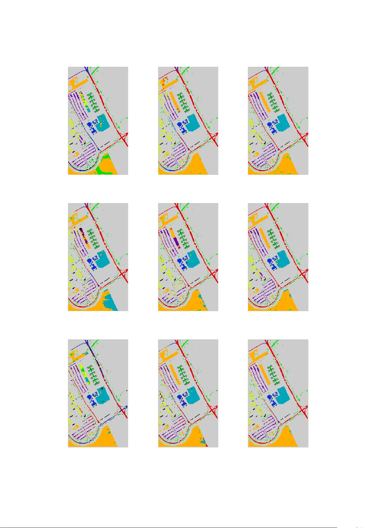
Effectiv e training of deep con v olutional neural net w orks for h yp ersp ectral image classification through artificial lab eling W o jciech Masarczyk, Przemysła w Głom b, Bartosz Grabowski, Mateusz Ostaszewski Institute of Theoretical and Applied Informatics, Polish Academ y of Sciences Bałtyc k a 5, 44-100 Gliwice, Poland Email: {wmasarczyk,przemg,bgrabowski,mostaszewski}@iitis.pl T elephone: +48 32 2317319 Abstract Hyp erspectral imaging is a rich source of data, allo wing for multitude of effectiv e appli- cations. Ho wev er, suc h imaging remains c hallenging b ecause of large data dimension and, t ypically , small p ool of av ailable training examples. While deep learning approaches hav e b een sho wn to b e successful in providing effective classification solutions, esp ecially for high dimensional problems, unfortunately they work best with a lot of lab elled examples av ailable. T o alleviate the second requirement for a particular dataset the transfer learning approach can b e used: first the netw ork is pre-trained on some dataset with large amount of training lab els av ailable, then the actual dataset is used to fine-tune the netw ork. This strategy is not straightforw ard to apply with h yp ersp ectral images, as it is often the case that only one particular image of some type or characteristic is av ailable. In this pap er, we prop ose and inv estigate a simple and effective strategy of transfer learning that uses unsup ervised pre-training step without lab el information. This approach can b e applied to many of the h yp ersp ectral classification problems. Performed exp erimen ts show that it is very effective at improving the classification accuracy without b eing restricted to a particular image type or neural netw ork architecture. The exp erimen ts were carried out on several deep neural net work arc hitectures and v arious sizes of lab eled training sets. The greatest improv emen t in o verall accuracy on the Indian Pines and Pa via Universit y datasets is ov er 21 and 13 p ercen tage p oints, resp ectiv ely . An additional adv antage of the prop osed approach is the unsup ervised nature of the pre-training step, which can be done immediately after image acquisition, without the need of the p oten tially costly expert’s time. Keyw ords: h yp ersp ectral image classification; deep learning; conv olutional neural netw orks; transfer learning; unsup ervised training sample selection 1 In tro duction Classification of h yp ersp ectral images (HSI) has many p oten tial applications, e.g. land co ver segmen tation [1], mineral identification [2], or anomaly detection [3]. The classification algo- rithms used include b oth general mo dels, e.g. the SVM [4], and dedicated approaches, taking in to account sp ectral prop erties or spatial class distribution [5]. Recently there hav e b een at- tempts to use Deep Learning Neural Netw orks (DLNN) for HSI classification. The motiv ation is that such metho ds hav e gained attention after achieving state of the art in natural image 1 pro cessing tasks [6]. Their unique ability to pro cess an image using a hierarchical comp osition of simple features learned during training makes them a p o w erful to ol in areas where manipulation of high-dimensional data is needed. While DLNN can achiev e very go od accuracy scores, they hav e the drawbac k of requiring a large amount of training data for estimation of mo del parameters. Such data is not alwa ys a v ailable, as it is common to ha ve a single HSI with just a handful of training lab els av ailable. T o bridge a gap b et ween this realistic scenario and DLNN netw ork requirements, we prop ose an approach that trains the DLNN in tw o stages, with the first – pre-training – stage using artificial lab els. In the remainder of this section, w e discuss the relev ant related, and in tro duce the motiv ation of our approach and state the hypothesis that is the base of our metho d. A num ber of DLNN architectures hav e b een prop osed, inspired by mathematical deriv ations and/or neuroscience studies. The Conv olutional Neural Netw orks (CNN) [7] are a sp ecial case of deep neural netw orks which were originally developed to pro cess images, but are also used for other types of data like audio. They combine traditional neural netw orks with biologically inspired structure in to a very effective learning algorithm. They scan m ultidimensional input piece by piece with a conv olutional window, which is a set of neurons with common weigh ts. Con volution windo w processes lo cal dependencies (features) in the input data. The output corresp onding to one conv olutional window is called a feature map and it can b e interpreted as a map of activit y of the given feature on the whole input. The CNN remain one of the most p opular arc hitectures for DLNN classification in use to da y . Other approaches include the generative architectures, e.g. the Restricted Boltzmann Ma- c hine (RBM) [8, 9], Auto encoders (AE) [10] or Deep Belief Netw ork (DBN) [11, 12]. Y et another p opular architecture is the Recurrent Neural Netw ork (RNN) whic h, through directed cycles b et w een units, has the p oten tial of representing the state of pro cessed sequence. They are ap- plicable e.g. for time series prediction or outlier detection. The most p opular types of RNN are Long Short-T erm Memory (LSTM) netw orks [13] and Gated Recurrent Units (GRUs) [14]. They improv e the original RNN architecture by dealing with explo ding and v anishing gradien t problem. F or classification of HSI data, the CNN is the most p opular arc hitecture chosen. In [15] the simple CNN architecture is adapted to HSI classification; the lac k of training labels is mitigated b y adding geometric transformations to a v ailable training data p oints. In [16] authors use three kinds of conv olutional windows: t wo of them are 3D conv olutions which analyse s patial and sp ectral dep endencies in the input picture, while the third is the 1D k ernel. Next the feature maps from these three types of con v olutions are stac ked one after the other and create join t output of this first part of the netw ork. The follo wing lay ers consist only of the one dimensional conv olutional kernels and residual connections. The authors of [17] in tro duce a parallel stream of pro cessing with an original approach for spatial enhancement of hypersp ectral data. The authors of [18] design a deep net work that reduces the effect of Hughes phenomenon (curse of dimensionality) and use additional unlabelled sample p ool to impro ve p erformance. In [19] authors propose an alternativ e arc hitecture called RPNet based on prefixed con volutional kernels. It com bines shallow and deep features for classification. Another architecture (MugNet) is prop osed in [20] with a fo cus on simplicit y of pro cessing for classification of hypersp ectral data with few training samples and reduced num b er of h yp erparameters. A yet another arc hitecture approach is used in [21] where a m ulti-branch fusion netw ork is introduced, whic h uses merging multiple branc hes on an ordinary CNN. An additional L2 regularization step is introduced to improv e the generalization ability with limited num b er of training samples. The work [22] prop oses a strategy based on m ultiple con volutional lay ers fusion. T wo distinct netw orks, comp osed of similar mo dules but different organization, are examined. Other architectures are also used. F or example in [23] authors utilize th e sequential nature 2 of hypersp ectral pixels and use some v ariations of recurrent neural netw orks – Gated Recurrent Unit (GR U) and Long-Short T erm Memory (LSTM) net w orks. Moreov er, in [24] one dimensional con volutional lay ers follow ed b y LSTM units were used. Chen et. al. [25] use artificial neural net works for feature extraction. They utilize stack ed auto enco ders (SAE) for feature extraction from pixels, and PCA for reduction of the sp ectral dimensionality of the training segments taken from the picture. Next, the logistic regression is p erformed on this spectral (SAE) and spatial (PCA) extracted information. Another approach [26] uses stack ed SAE for an application study – detection of a rice eating insect. RNN architectures are also employ ed, as they are suitable for pro cessing the sp ectral vector data. The work [27] applies sequen tial sp ectral pro cessing of h yp ersp ectral data, using a RNN supp orted by a guided filter. In [28] authors use the multi- scale hierarc hical recurrent neural net works (MHRNNs) to learn the spatial dep endency of non- adjacen t image patches in the tw o-dimension (2D) spatial domain. Another idea to analysing HSI is spatial–spectral metho d in which net w ork takes information not only from spectrum bands but also from spatial dep endencies of image [16]. A significant problem in practical h yp erspectral classification is the small num b er of training samples. It is related to the difficulty of obtaining verified lab els [1], as often each pixel must b e individually ev aluated b efore lab elling. Therefore, a reference hypersp ectral classification exp erimen t may assume num b er as lo w as 1% av ailable samples per class [2]. A n um b er of approac hes has b een exploited to deal with this difficulty , e.g. including combining spatial and sp ectral features [29], additional training sample generation [30], extending the classification algorithm with segmentation [31], or employing Activ e Learning [32]. F or the DLNN classification, the lac k of high volume of training data is a serious complication, as they typically require a lot of data to achiev e high efficiency . Optimal use of DLNN in HSI classification w ould require learning them with just a few lab elled samples. This ma y b e obtained b y searching for well-tailored architecture for sp ecific task [15], how ever such approach requires relativ ely big v alidation set to obtain meaningful results. The other approach is to expand the a v ailable training set. It may be achiev ed either by artificially augmen ting training set or using differen t dataset as a source for pre-training [33]. Another approach is to add a regularization step to impro ve the generalization abilit y with limited n umber of training samples [21]. A simplification of the netw ork architecture for classification with few training samples is employ ed in the MugNet netw ork [20]. Finally , where p ossible, the transfer learning approach is used, e.g. [34]. The transfer learning [35] uses training samples from tw o domains, whic h share common c haracteristics. A netw ork is first pre-trained on the first domain, whic h has plentiful supply of training samples but do es not solve the problem at hand. Then, the training is up dated with the second domain, which adapts the weigh ts to the actual problem. T ransfer learning is simple to apply in the case of conv olutional neural netw orks (CNNs). In [36], authors compared different versions of transfer learning for CNNs in the case of natural images classification. They studied its effects dep ending on the num b er of transferred lay ers and whether they were fine tuned or not as well as dep ending on the differences b et ween the considered datasets. In [37], authors used transfer learning on CNNs to recognize emotions from the pictures of faces. Other uses include ev aluating the level of p o vert y in a region given its remote sensing images [38] and computer-aided detection using CT scans [39]. There hav e b een applications of transfer learning in the general remote sensing (not-hypersp ectral) images. In [40] deep learned features are transferred for effective target detection; negative b oot- strapping is used for impro ving the conv ergence of the detector. A similar approac h is applied in [41] where RNN net work trained on m ultisp ectral city images is used to derive features for studying urban d ynamics across seasonal, spatial and annual v ariance. The authors of [42] study the p erformance of transfer learning in tw o remote sensing scene classifications. The results show 3 that features generalize w ell to high resolution remote sensing images. As the work [43] sho ws, transfer learning can b e applied in remote sensing using RNN arc hitectures also. Recen tly , transfer learning has b een also applied to the HSI data. In [34], authors applied it for CNNs originally used for classifying well kno wn remote sensing hypersp ectral images to clas- sify images acquired from field-based platforms and regarding a differen t domain. The authors of [44] use a in termediate step of sup ervised similarit y learning for anomaly detection in unla- b elled h yp ersp ectral image. A different approach to transfer learning is prop osed in [45] which explores the high lev el feature correlation of tw o HSI. A new training principle simultaneously pro cesses b oth images, to estimate a common feature space for b oth images. A yet another approac h is prop osed in [46] where HS I sup erresolution is achiev ed using supp orted high reso- lution natural image. This natural image is used as a training reference, which is later adapted to HSI domain. In [47], iterative pro cess com bines training and up dating the currently used training lab el set. T wo sp ecialized architectures (for spatial and sp ectral pro cessing) are used. The training iteratively extends the current lab el set, starting from the initial exp ert’s labels. The ab o ve approaches do not apply to the arguably most p opular practical scenario, where only a single HSI with a handful of lab els is av ailable. Moreov er, getting the training lab els often requires additional resources (e.g. exp ert consultation and/or site visit). It is thus desirable to ha ve unsup ervised metho ds for realization of the pre-training step. Authors of [48] use outlier detection and segmentation to provide candidates for training of target detector in HSI. This information is used to construct a subspace for target detection by transfer learning theory . This shows the p oten tial of using an unsup ervised approach, how ever limited to separation of target/anomaly p oin ts from the background. In the w ork of [33], a separate clustering step is used for generation of pseudo-lab els, using Dirichlet pro cess mixture mo del. The netw ork is trained on the pseudo-lab els, then the all but last lay ers are extracted, and the final netw ork is trained on the originally provided training lab els. While this scheme is shown to b e effectiv e in the presented results, it relies on a complex non-neural prepro cessing and tailoring the DLNN configuration to each dataset separately . Also, the effect of size of lab el areas and effects on differen t arc hitectures are not in vestigated. W e show that similar gains can b e made with a simpler prepro cessing, independent of the DLNN architecture chosen. The authors of [49] prop ose to use a sparse co ding to estimate high level features from unlab elled data from different sources. This approach do es not require training data, but is tailored to the case where multiple inputs are av ailable, preferably with diverse con tents. T o close the gap b et ween data inefficient deep learning mo dels and practical applications of HSI we prop ose a metho d which takes adv an tage of abundan t unlab elled data p oin ts present on HSI images. Precisely , w e state a hypothesis: Spatial similarity of unlab elled data p oin ts can b e utilized to gain accuracy in hypersp ectral classification. T o corrob orate our h yp othesis, w e construct a simple clustering metho d that assigns artificial lab el to each pixel on the image based on its spatial lo cation. This artificial dataset is used to pre-train deep learning classifier. Next the model is fine-tuned with original dataset. Through series of exp eriments we show sup eriorit y of the prop osed approach o ver the standard learning pro cedure. Our approach is motiv ated by tw o kno wn phenomena: cluster assumption [50] and regularization effect of noise in classes [51, 52, 53]. W e note that many of remote sensing images share common prop erties, most notably the ‘cluster assumption’ – pixels that are close to one another or form a distinct cluster or group frequently share the class lab el. Additionally , due to the simplistic form of our clustering metho d, w e purp osefully introduce noise in lab els used during pre-training phase, ho wev er as shown in [51] this lab el noise has little to no effect on final accuracy , as long as n umber of prop erly lab elled examples scales prop ortionally whic h is our case. 4 2 Materials & Metho ds Our metho d is to b e applied in the following case: 1. Classification of pixels from a remote sensing hypersp ectral image; 2. Neural netw orks used as a classifier; 3. F ew training lab els av ailable. In such situation, we prop ose to augment the training with a pre-training step that uses artificial lab els, which are indep enden t of the training lab els. Inclusion of this pre-training step can b e view ed as a mo dification of a transfer learning approach. Conv en tional transfer learning in this case would use a related dataset (source domain) with abundance of lab els to pre-train, then the current dataset (target domain) to fine-tune. In our case, the source domain consists of ev ery p oint in the h yp erspectral image, while the target domain is comp osed of only the labelled samples. In the remainder of this Section w e discuss: the spatial structure of hypersp ectral images and the characteristics of neural netw ork that make this approach feasible, and the details of its application. W e also describ e the exp erimen ts used to test the prop osed approach. 2.1 Spatial structure of h yp ersp ectral images It is well-kno wn that remote sensing h yp ersp ectral images con tain spatial structure, that can b e exploited to impro ve clas sification scores when only a few training samples are av ailable [54, 31, 5, 55, 30]. A segmentation can b e applied to prop ose candidate pixels for lab elling with high confidence [54] or identify connected components for label assignmen t [31]. Class training samples can b e extended through mo derated region growing [5] or spatial filtering combined with spatial- sp ectral Lab el Propagation [55]. Finally , disagreement b et ween spatial and sp ectral classifiers can b e used to prop ose new samples [30]. A qualitative in vestigation of this phenomenon shows that h yp ersp ectral pixels close to one another, whether spatially or sp ectrally , are lik ely to hav e the same class lab el, th us fulfilling the ‘cluster assumption’ [50]. This effect often leads to a blob- lik e structure of a hypersp ectral dataset, observ ed in many hypersp ectral classification problems (e.g. land cov er lab elling in remote sensing, paint iden tification in heritage science, scene analysis in forensics). A single class with samples in differen t parts of an image can b e made of a n umber of blobs, which differ from each other b ecause of, e.g., non-uniformity in class structure (e.g. the same class can contain differing crop types), sp ectral v ariations (e.g. same crop in tw o areas can ha ve differing prop erties due to sunlight exp osure, soil type) or acquisition conditions (e.g. level of lighting, shado ws). 2.2 Emergence of data-dep enden t filters in neural net work training During training, subsequen t lay ers of a deep neural netw ork form a represen tation of a lo cal input data structure [56]. Given a data source, this representation, esp ecially on low er lay ers, can b e remark ably similar across different dataset. F or example, in the problem of natural image classification the learned k ernels resemble a Gab or filter bank [6, 57], indep enden t of class set. This form of a filter can b e shown to arise indep endently when indep enden t comp onen ts [58] or an effective sparse co de [59] for natural images is estimated. Another case where data-dep enden t filters emerge is the pretext task approac h, e.g. [60, 61], where the netw ork first learns to predict the input sequence without class lab els, which are introduced at a fine-tune stage for to get the final classification mo del. Apparen tly the deep neural net works are able, at le ast in part, to extract an efficient class-indep enden t data representation. This phenomenon has not b een 5 studied for hypersp ectral images, how ever, it can be argued that similar class-indep endent but data-dep enden t representation is b eing learned in training for hypersp ectral image classification. 2.3 Metho ds used for prop osed artificial lab elling approach Our metho d for creating artificial lab els for the pre-training step is a simple segmentation al- gorithm whic h assumes the lo cal homogeneity of samples’ sp ectral characteristics. It works by dividing the considered image in to k rectangles, where eac h of these rectangles has its o wn lab el. F or an image of height h and width w , w e divide its heigh t into m roughly equal parts and its width in to n roughly equal parts, so that k = m · n . W e then get k rectangles, where eac h one’s height equals appro ximately h/m , while its width equals approximately w/n . Each of these rectangles defines a different artificial class with a different lab el. A schematic is presented in Figure 1. The function of artificial lab els is for the net work to learn class-indep endent blob patterns presen t in the data. This fo cuses the netw ork training in the fine tuning on the actual training lab els, with the netw ork ‘orien ted’ to wards the features of the current image. It can also b e of adv antage in situations when a class is comp osed of multiple blobs, and not all of them hav e samples in the training set. In that case sufficien tly correct lab elling is unlikely to be obtained [62] with just the training samples, but the prop osed grid structure forces the net work to es timate features for the whole image. An additional adv an tage of this approach is to shift the p oten tially time consuming pre-training from the exp ert lab elling moment to the acquisition momen t. In other w ords, netw ork training do es not need to be held bac k un til the exp ert’s labels are a v ailable, but can commence right after the image is recorded. 2.4 Selected netw ork architectures In our exp eriments three architectures were tested, based on [16, 15, 63]. All three share a com- mon approach to exploit lo cal homogeneity of hypersp ectral images, how ever each one has its unique strengths and weaknesses making them an interesting testb ed for the universalit y of the prop osed metho d. The first architecture [16] features relativ ely high num b er of conv olutional la yers which mi gh t b e helpful in transfer learning application. The second architecture [15], to the b est of authors knowledge, is one of the b est netw orks that are trained on limited num b er of samples p er class. How ev er due to its constrained capacity , it may not b enefit as muc h from the pre-training phase. The last of the considered con volutional neural netw orks [63] is concep- tually the simplest of the three, which allo ws us to test our approac h using more conv entional con volutional arc hitecture. 2.5 Exp erimen ts This subsection describ es the exp erimen ts ev aluating the prop osed approach. W e inv estigate the p erformance of the artificial lab el pre-training in the following four exp erimen ts: 1. Exp erimen t 1 ev aluates the accuracy improv ement ac hieved b y using the metho d. 2. Exp erimen t 2 inv estigates the v ariabilit y introduce d by the size and shap e of the patc hes used to define artificial classes, using one of the datasets from Exp erimen t 1. 3. Exp erimen t 3 is an additional inv estigation of the observed phenomenon that big patches (larger area, smaller total n umber of classes) p erform worse than little ones (smaller area, larger total num b er of classes), done using a different dataset. 6 Pre t ra i n i n g Ev a l u a t i o n F i n e - t u n i n g P r e t ra i n i n g r e s u l t F i n a l re su l t A r t i f i ci a l l a b e l s T ru e l a b e l s T r a i n i n g l a b e l s su b se t H y p e r sp e ct ra l d a t a N e t w o rk a r ch i t e ct u re , h y p e rp a ra m e t e r s Figure 1: The ov erview of the unsup ervised pretraining algorithm prop osed in this work. First, the netw ork is pretrained on grid-based scheme of artificially assigned lab els. The netw ork weigh ts are then fine-tuned on a limited set of training samples selected from true lab els, consistent with t ypical hypersp ectral classification scenario. 4. Exp erimen t 4 is an examination of a claim ab out the emergence of data-indep endent rep- resen tations during neural net work training using prop osed artificial lab elling sc heme. In the following subsections, the detailed descriptions of the conducted exp erimen ts are given, while in the Section 3 we present the results of the exp erimen ts. 2.5.1 Exp erimen t 1 In this exp erimen t, the prop osed approach is ev aluated using different hypersp ectral images and neural netw ork architectures to prov e its robustness. F or the exp erimen t, we hav e used tw o w ell-known hypersp ectral datasets: Indian Pines and P avia Univ ersity . The Indian Pines dataset was collected by the A VIRIS sensor ov er the Northw est Indiana area. The image consists of 145 × 145 pixels. Each pixel has 220 sp ectral bands in the frequency range 0.4–2.5 × 10 − 6 m. Channels affected by noise and/or w ater absorption were remov ed (i.e. [104–108], [150–163], 220), bringing the total image dimension to 200 bands. The reference ground truth contains 16 classes representing mostly different t yp es of crops. T o b e consistent with exp erimen ts p erformed in [16], we c ho ose only 8 classes. 7 The Pa via Univ ersity dataset w as collected by the ROSIS sensor ov er the urban area of the Univ ersity of Pa via in Italy . This image consist of 610 × 340 pixels. It has 115 sp ectral bands in the frequency range from 0.43 to 0.86 × 10 − 6 m. The noisiest 12 bands were remo ved, and remained 103 w ere utilized in the exp erimen ts. Ground truth includes 9 classes, corresp onding mostly to different building materials. The tw o datasets w ere sub jected to a feature transformation. F or a given dataset, the mean m b of each hypersp ectral band b were calculated. In the case of eac h dataset, and for each given pixel x and band b , the corresp onding mean m b w as subtracted, x ( b ) := x ( b ) − m b . F or this exp erimen t, all three of the previously introduced neural netw ork architectures were used. As discussed previously , the training w as divided into pre-training and fine-tuning stages. In pre-training, the data was lab elled through assigning an artificial class to eac h blo c k within a grid of dimensions 5 × 5 . No ground truth data was used at this stage. In the fine-tuning stage, a selected n umber of ground truth lab els w as used. The num b er of training samples from eac h class w as set at n = 5 , 15 , 50 . This allow ed to observe the p erformance b oth in typical hypersp ectral scenarios (small num ber of classes used) and deep netw ork scenarios (larger num b er of samples p er class av ailable). Because the classification accuracy dep ends on the training set used in fine-tuning each exp erimen t was rep eated n = 15 times for error rep orting. The p erformance is rep orted in Overall Accuracy (O A) after fine tuning. Additionally , A v erage Accuracy (AA) and κ co efficien t were insp ected and improv ements verified with statistical tests. 2.5.2 Exp erimen t 2 The second experiment inv estigates the v ariability introduced b y the size and shape of the patc hes used in artificial lab elling. F or this exp erimen t only the Indian Pines image introduced in Exp erimen t 1 was used, as it is the more challenging of the t wo in tro duced datasets. As was the case with the previous exp erimen t, the mean w as subtracted. The netw ork in vestigated is the architecture based on [16], c hosen b ecause it has the most p otential to b e affected by the transfer learning pro cess. In this exp erimen t, first the grid size was inv estigated. The dimensions of the patches, v aries from 2 × 2 , which equals 4 artificial classes, up to 72 × 72 , 5184 artificial classes. F urthermore, another w ay of creating artificial labels is considered. The image is divided into the giv en n umber of vertical stripes. Visualisation of different artificial lab elings is presented in Figure 2. The inv estigated patches were created by dividing horizontal and vertical side of an image in to w = 2 , 3 , 5 , 7 , 9 , 15 , 19 , 25 , 29 , 36 , 39 , 48 , 72 equal parts. The vertical strip es were created by dividing horizontal side of an image in to s = 2 , 5 , 9 , 16 , 25 , 36 , 49 , 81 equal parts (so in the case of s = 2 , there are only 2 classes lo cated to the right and left of a single vertical line). The vertical strip es w ere included to observe whether the pixel distance affects the p erformance – for patc hes, all the pixels share similar neigh b ourho od; for strip es, the top and b ottom pixels ha ve a notable spatial separation and, arguably , the distant pixels should not b e marked with the same class lab el without prior knowledge of spatial class distribution. Note that in case of patches made b y dividing eac h side of an image into w = 29 , 36 , 39 , 48 , 72 equal parts the size of a square patch is smaller than the size of a pro cessing window 5 × 5 in teste d architecture. That means no sample fed to a netw ork during pre-training phase has a coherent class representation (i.e. a single class presen t in the window). This exp erimen t w as p erformed with 5 training samples p er class and 50 exp erimen t runs for each grid density and the n umber of strip es. 2.5.3 Exp erimen t 3 In this exp erimen t, we test the hypothesis that the more numerous patc hes’ division pro duces a b etter pre-training set than the less n umerous ones. W e in vestigate this using a sp ecially designed 8 (a) Grid 3 × 3 (b) Strip es 5 Figure 2: Scheme of creating artificial classes on Indian Pines dataset. F rom left: grid of 9 artificial classes (a) , v ertical strip es with 5 artificial classes (b) . Artificial classes for P a via Univ ersity dataset were created analogically . h yp ersp ectral test image. In this exp erimen t, w e use the image of pain ts from museum’s collection. This dataset [64] w as collected b y the SPECIM hypersp ectral system in the Lab oratory of Analysis and Nondestructiv e In vestigation of Heritage Ob jects (LANBOZ) in National Museum in Krakó w. This image consist of 455 × 310 pixels. Each pixel has 256 spectral bands in the frequency range from 1000 to 2500 nm. Ground truth consists of manual annotations of differen t green pigments used in the mixture of paints for v arious painting regions. The image of oil paints on pap er was used, selected from four av ailable, as it was considered one of the more challenging of the images. The lay out of classes present in this image was esp ecially designed to verify hypersp ectral classifiers. The different chemical comp ositions of the paints used introduce v ariations of class sp ectra, yet at the same time all paints are v ariations of the green pigment with more or less greenish h ue. The classification problem is th us difficult, but not exceedingly so. Regular grid la yout, with different thickness of paints and fragments where one pigment ov erpaints another, in tro duce spatial diversit y in the sp ectra. Since the image is artificially created, ground truth can b e precisely marked. The original purp ose of the image w as to ev aluate iden tification of copp er pigmen ts, difficult to differentiate by other (non-hypersp ectral) sensors. Here we tak e adv antage of its regularity by complementing the original ground truth ( n GT = 5 classes) with a joined set ( n GT − 2 = 2 classes) and split set ( n GT − 10 = 10 classes). Those tw o sets of mo dified ground truth allow us to compare the prop osed grid scheme, as tested in exp erimen ts 1 and 2, with a ground truth based pre-training with more and less classes than the original set. W e argue that the regular la yout of this image is more suited for this exp eriment than e.g. Indian Pines or P avia Univ ersity images; usage of additional dataset allows us to further verify the generalization p oten tial of our approach. In the case of this dataset, the mean was subtracted as in the case of the previous exp eriments. A dditionally , the standard deviation σ b of each hypersp ectral band b was calculated and then all pixels were divided by the corresp onding standard deviation v alue σ b , x ( b ) := x ( b ) σ b . In this exp erimen t, as in the previous one, the neural netw ork based on [16] was used. T raining size was equal to 5 training samples p er class and there were 50 exp erimen t runs for each examined case. The following cases were in vestigated: 9 (a) Pain ting (b) GT (c) GT-2 (d) GT-10 Figure 3: Sc heme of creating artificial classes on Pigmen t dataset. F rom left: false-colour RGB (bands 50, 27, 17) image of the painting (a) , original class lab els (b) , classes artificially joined in to 2 sets (c) , classes artificially split into 10 sets (d) . Dark rectangles denote background, excluded from the exp erimen t. 1. The p erformance of DLNN with pre-training p erformed with 2 classes prepared from joining the ground truth classes (GT-2). 2. The p erformance of DLNN with pre-training p erformed with 10 classes prepared by split- ting the ground truth classes (GT-10). 3. The p erformance of DLNN without pre-training (GT). 4. The performance of DLNN with pre-training with artificial patches of size 5 × 5 , 20 × 20 , 30 × 30 . 2.5.4 Exp erimen t 4 In this exp erimen t, we examine the claims from subsection 2.2 ab out the emergence of data- dep eneden t represen tations during neural netw ork training using prop osed artificial labelling sc heme with noisy labels. T o this end, we visualised in ternal net work parameters resulting from net work training using t-SNE algorithm [65]. In the exp erimen t, we used neural netw ork arc hitecture based on [16] and the Indian Pines dataset describ ed in subsection 2.5.1. W e trained the netw ork on the dataset using the following scenarios: 1. The netw ork w as trained using 1600 lab elled samples, with 200 samples p er class. This scenario represents the neural netw ork trained with abundant information ab out the data – unrealistic, but conv enien t from the p oin t of netw ork’s requiremen ts. 2. The netw ork was trained using 40 lab elled samples, with 5 samples p er class. This scenario represen ts the neural netw ork trained with v ery limited information about the data – realistic, but difficult learning problem. 3. The netw ork was trained using only the artificial lab els created as explained in subsec- tion 2.3. Therefore, the netw ork did not ’see’ the true lab els and could create the internal represenations only based on the noisy lab els provided for training. 4. The netw ork was trained using the complete pretraining-finetuning scheme introduced in this section. That is, first it was pretrained using artificial lab els as in p oint 3, and then 10 all lay ers except the last was finetune using the training set analogous to the one from p oin t 2. This scenario was introduced to help explain the impact of the finetuning step in our approach. As a result, we obtain 4 trained neural netw orks. As a next step, using v alidation dataset w e extract the activ ations of the next-to-last lay ers of the considered netw orks, and use t-SNE algorithm, which is used to visualise high-dimensional data, to learn if the la yers right b efore the classification lay ers of the netw orks did learn useful data representations. 3 Results This Section presents the results of exp erimen ts introduced in subsection 2.5. 3.1 Exp erimen t 1 The first exp eriment’s results are presented in T able 1. Each column presents the result for one t yp e of netw ork, each ro w for a set dataset and the n umber of training examples. Each table cell presen ts the results with and without pre-training, in p ercen t of Overall Accuracy , including the standard deviation of the result. The results from T able 1 were computed from a batch of n = 15 indep enden t runs for each case. The sp ecific v alue of n was chosen to provide robust result, after a set of preliminary runs with different n v alues. A Mann–Whitney U test was p erformed on the results to confirm statistical significance of the improv emen t gained with the prop osed metho d. As Overall Accuracy can b e sensitive to class imbalances, A verage Accuracy and κ co efficient w ere computed for additional verification, and were inspected for negative p erformance. The presented results sho w that application of the prop osed metho d leads to definite and consisten t improv ement in accuracy across different images, num b er of ground truth lab els used and netw ork arc hitectures. In all but one case, the improv ement is statistically significan t, and in some cases approac hes 20 p ercen tage p oin ts. The most challenging is scenario with 5 training samples p er class. Even a verage o verall accuracy ac hieved b y architecture originally examined on small training set [15] do es not exceed 67% on Indian Pines dataset. After the application of the proposed metho d, p erformance improv es up to 72.8% OA. The most improv ement is seen in the architecture [16], namely on IP dataset with only 5 training samples p er class in fine- tuning pro cedure, it improv es from a verage 52.62 OA to 74.04 O A. This is to b e exp ected as this arc hitecture has the most p oten tial to b enefit from additional training samples. Considering these improv emen ts, it can b e summarized that the results of the exp eriment supp ort stated h yp othesis and the v alidity of the prop osed approac h. The qualitativ e ev aluation of selected realizations (corresp onding to the median score) is presented in Figures 4 and 5. 3.2 Exp erimen t 2 The results of the exp erimen t are presen ted in T able 2. F or eac h grid size or the num b er of strip es, the ov erall accuracy and the standard deviation are giv en. These statistics are based on 50 exp erimen t runs for each artificial lab elling scheme. It can b e seen that the the score rises sharply until the num b er of artificial classes reaches appro ximately the num b er of original classes (at 5 × 5 , note that the original IP ground truth lea ves a sizeable p ortion of bac kground unmarked, whic h most probably would con tribute some additional classes if marked). After that v alue, there’s a declining trend. It can b e noted that the scores are higher with smaller patches. It seems viable to form a conclusion that when the original class n umber is unknown, it is b etter to o verestimate than underestimate their num b er. 11 T able 1: The result of the first exp erimen t. Each row presents Overall A ccuracy (O A), A v erage Accuracy (AA) and Cohen’s k appa ( κ ) for given scenario. IP denotes the Indian Pines dataset, PU the P a via Univ ersity; further differentiation is for num b er of samples p er class in fine-tuning. Accuracies are given as av erages with standard deviations with and without pretraining for the three in v estigated net w ork arc hitectures. arc hitecture [16] arc hitecture [15] arc hitecture [63] no pretraining pretraining no pretraining pretraining no pretraining pretraining IP 5/class O A: 52 . 62 ± 4 . 4 74 . 04 ± 4 . 1 † 66 . 15 ± 4 . 5 72 . 80 ± 3 . 2 † 50 . 05 ± 5 . 1 63 . 52 ± 4 . 2 † AA: 58 . 15 ± 2 . 9 78 . 83 ± 2 . 6 † 71 . 42 ± 3 . 9 78 . 60 ± 3 . 0 † 53 . 66 ± 3 . 0 65 . 86 ± 3 . 6 † κ : 0 . 45 ± 0 . 04 0 . 69 ± 0 . 05 † 0 . 60 ± 0 . 05 0 . 68 ± 0 . 04 † 0 . 41 ± 0 . 05 0 . 57 ± 0 . 05 † IP 15/class O A: 67 . 58 ± 3 . 2 87 . 04 ± 2 . 4 † 82 . 61 ± 2 . 8 87 . 04 ± 2 . 1 † 64 . 18 ± 2 . 8 75 . 30 ± 1 . 7 † AA: 73 . 82 ± 2 . 7 90 . 41 ± 1 . 5 † 87 . 07 ± 1 . 8 90 . 97 ± 1 . 5 † 67 . 54 ± 2 . 5 78 . 40 ± 2 . 1 † κ : 0 . 62 ± 0 . 03 0 . 85 ± 0 . 03 † 0 . 79 ± 0 . 03 0 . 85 ± 0 . 02 † 0 . 58 ± 0 . 03 0 . 71 ± 0 . 02 † IP 50/class O A: 80 . 51 ± 4 . 8 93 . 66 ± 1 . 3 † 93 . 75 ± 1 . 2 94 . 65 ± 1 . 0 81 . 39 ± 1 . 1 87 . 06 ± 0 . 9 † AA: 87 . 48 ± 2 . 6 95 . 81 ± 0 . 8 † 95 . 86 ± 0 . 7 96 . 62 ± 0 . 8 † 85 . 10 ± 0 . 9 90 . 38 ± 1 . 1 † κ : 0 . 77 ± 0 . 05 0 . 92 ± 0 . 02 † 0 . 92 ± 0 . 01 0 . 94 ± 0 . 01 0 . 78 ± 0 . 01 0 . 85 ± 0 . 01 † PU 5/class O A: 67 . 47 ± 6 . 5 80 . 08 ± 7 . 0 † 73 . 31 ± 4 . 1 80 . 33 ± 5 . 2 † 65 . 55 ± 3 . 8 74 . 34 ± 7 . 0 † AA: 76 . 56 ± 3 . 1 87 . 66 ± 2 . 9 † 84 . 67 ± 2 . 6 88 . 86 ± 3 . 2 † 64 . 39 ± 2 . 4 76 . 92 ± 3 . 7 † κ : 0 . 60 ± 0 . 07 0 . 75 ± 0 . 08 † 0 . 67 ± 0 . 05 0 . 76 ± 0 . 06 † 0 . 56 ± 0 . 04 0 . 68 ± 0 . 08 † PU 15/class O A: 83 . 63 ± 2 . 7 91 . 87 ± 3 . 3 † 88 . 21 ± 2 . 9 91 . 96 ± 2 . 6 † 75 . 50 ± 2 . 4 89 . 33 ± 3 . 4 † AA: 89 . 48 ± 1 . 1 94 . 65 ± 1 . 0 † 93 . 40 ± 1 . 1 95 . 01 ± 0 . 8 † 77 . 59 ± 1 . 2 89 . 95 ± 1 . 8 † κ : 0 . 79 ± 0 . 03 0 . 90 ± 0 . 04 † 0 . 85 ± 0 . 04 0 . 90 ± 0 . 03 † 0 . 69 ± 0 . 03 0 . 86 ± 0 . 04 † PU 50/class O A: 93 . 40 ± 1 . 4 97 . 86 ± 0 . 5 † 96 . 08 ± 0 . 9 96 . 84 ± 1 . 2 ‡ 87 . 79 ± 1 . 7 96 . 55 ± 0 . 5 † AA: 95 . 47 ± 0 . 7 98 . 13 ± 0 . 3 † 97 . 09 ± 0 . 5 97 . 90 ± 0 . 4 † 89 . 05 ± 0 . 9 96 . 37 ± 0 . 3 † κ : 0 . 91 ± 0 . 02 0 . 97 ± 0 . 01 † 0 . 95 ± 0 . 01 0 . 96 ± 0 . 02 ‡ 0 . 84 ± 0 . 02 0 . 95 ± 0 . 01 † † , ‡ Statistically significant improv ement, ev aluated with Mann–Whitney U test, with P < 0 . 01 ( † ) or P < 0 . 05 ( ‡ ). In the latter case, it is p ossible that even a chance guess w ould pro vide a satisfactory performance. The strip es do not form as go od a training set as rectangular grid, which confirms the initial supp osition that artificial classes should b e confined to lo cal areas. Some improv emen t how ev er is still seen, which supp orts our ov erall prop osition, that general artificial lab elling can b e used for improving the DLNN p erformance without precise estimation of the artificial class patch size. 3.3 Exp erimen t 3 T able 3 presents the results of the third exp erimen t. The ov erall accuracy w as calculated based on n = 50 runs for eac h examined scenario. Here, the original p erformance (GT) can b e significan tly improv ed by the grid-based artificial lab elling (see results for 5 × 5 , 20 × 20 , 30 × 30 ). How ev er, in this case the p erformance gain can b e confronted with a lab el dataset created from ground truth data (GT-2, GT-10). As can b e exp ected, the ground truth data provides a higher p erformance; how ev er, the artificial lab elling pro vides half of that gain with no prior information needed. The ground truth exp erimen ts GT-2 and GT-10 also confirm the observ ation that classes split is a b etter option than joining. The latter observ ation provides an additional supp ort to the conclusion that more small classes (dense grid) is preferable than few large ones (sparse grid). 12 T able 2: The second exp erimen t results. Grid density describ es num b er of rectangular patches which represent artificial lab els for pre-training phase. Num of strip es denotes num b er of vertical strip es which represent artificial lab els for pre-training phase. Accuracies are giv en as Overall A ccuracy for learning of the net work based on [16] with transfer learning on the Indian Pines dataset. Grid density / mo del O A Num of strip es / mo del O A (2x2) 61 . 88 ± 4 . 5 2 58 . 53 ± 4 . 9 (3x3) 64 . 45 ± 4 . 1 5 67 . 68 ± 4 . 4 (5x5) 75 . 05 ± 4 . 3 9 68 . 58 ± 3 . 9 (7x7) 72 . 33 ± 4 . 4 16 69 . 25 ± 3 . 7 (9x9) 74 . 06 ± 3 . 6 25 69 . 09 ± 3 . 6 (14x14) 74 . 13 ± 3 . 7 36 69 . 23 ± 3 . 3 (19x19) 73 . 24 ± 3 . 9 49 70 . 08 ± 4 . 0 (24x24) 73 . 43 ± 4 . 0 81 68 . 41 ± 4 . 3 (29x29) 70 . 19 ± 4 . 6 (36x36) 69 . 88 ± 4 . 3 (39x39) 68 . 69 ± 4 . 4 (48x48) 69 . 25 ± 3 . 2 (72x72) 66 . 70 ± 3 . 3 T able 3: The third exp erimen t results. Ev aluation of pretraining on Pig- men ts dataset using the prop osed approach and classes created from ground truth. The ob jective w as to collate the p erformance of artificial lab els of differen t sizes with those created through splitting or joining the ground truth. Exp erimen t setting GT a (5x5) b (20x20) b (30x30) b GT-2 c GT-10 c O A 61.15% 68.35% 75.70% 73.99% 75.70% 85.40% a No pretraining. b Pretraining with artificial classes (prop osed metho d). c Pretraining with mo dified ground truth classes (verification). 3.4 Exp erimen t 4 The results of the exp erimen t are presen ted in Figure 6. As exp ected, the net work trained using 1600 true-lab eled samples generated go o d in ternal represen tations, whic h can b e seen b y the go od separability of the classes. In contrast, neural netw ork trained using only 5 samples p er class did not generate representations allo wing the separation of samples of different classes. In the case of scenario 3, we can clearly see that the classes were b etter separated when compared with scenario 2, though of course not as go od as in scenario 1. Moreov er, the authors did not observ e any noticeable differences b et ween scenarios 3 and 4. W e argue that the presen ted results provide some suggestion that during neural netw ork training using prop osed artificial lab elling scheme there is an emergence of useful data-related represen tations even b efore the fine-tuning step. 13 4 Discussion Our results confirm the v alidit y of our prop osition: a simple artificial lab elling through grouping of the samples based on a lo cal neighbourho o d provides an efficient transfer learning scheme. It brings significant improv ements of accuracy across datasets and DLNN configurations. The re- sults for differen t datasets, which ha ve distinctive ground truth lay outs suggest that it is not the random alignment with the regularity of a particular ground truth pattern. It is also seen that the local structure is important, as seen in the adv antage of grid division o ver strip e division. The generally b etter p erformance of higher ov er low er num b er of artificial classes suggests an expla- nation in that for transfer learning, it is not as imp ortan t to lo cate the exact num b er of classes, but to isolate and learn their comp onents, p erhaps for b etter in ternal feature representation. W e view the main adv antage of the prop osed metho d as enhancing the training of a neu- ral netw ork for hypersp ectral remote sensing classification. The prop osed pre-training offers a n umber of b enefits: 1. Enhance the training of neural netw orks in h yp erspectral classification scenario. With low n umber of training samples in typical scenarios (e.g. 5 − 15 /class, sometimes even less) the num b er of netw ork free parameters can b e several orders of magnitude higher than the training data, which p oses a risk of ov ertraining. 2. Through splitting the training into tw o phases, it can b e used to shift some of the com- putational burden of netw ork training to the time b efore an exp ert is called in to p erform lab elling, and make more effective use of his or hers time. 3. Larger num b er of training samples av ailable can b e of use in case differen t netw ork archi- tectures are compared for the same problem, or during the searching the h yp erparameter space. An op en question is whether a clustering algorithm, lik e [33] or outlier segmentation [48] could b e adapted here leading to greater efficiency . It is probable that a more complex artificial lab elling algorithm could outp erform the prop osed solution; ho wev er even in that case, a simple, generally applicable heuristic that improv es p erformance can b e of v alue. Our approach has common motiv ation with self-taugh t learning [49], where we w ant the classifier to derive high- lev el input represen tation from the unlab elled data; ho wev er w e use the same data for b oth training stages and instead c hange the lab el set. It also av oids com bining neural and non-neural approac hes, and preven ts introducing additional assumptions through the manual selection of the latter. A qualitative examination of the pre-training results shows that some class structure is visible after pre-training (see examples in Figure 7). No iden tifiable features of this structure ha ve b een noticed when in vestigating pre-training images when asso ciated with b etter or worse final (after fine-tuning) results. Ho wev er, the general level of structure visible after pre-training relates to the final p erformance. The net work architecture based on the work [63] is b est in learning the artificial classes grid and also the w orst at the final classification. The other tw o netw orks based on the w orks [16, 15] hav e more complex pre-training results and corresp ondingly b etter final results. This suggests that the training scheme and/or netw ork architecture functions as a form of regularization that preven ts o vertraining, and that the pre-training classification result can b e p ossibly used to con trol pre-training and av oid ov ertraining to o. The emergence of partial class structure in the pre-training phase – which do es not use ground truth, hence can b e viewed as unsup ervised pro cessing – also suggests that this approach can b e adapted to solve unsup ervised tasks, e.g. clustering or anomaly detection. 14 T o provide additional v erification, we’v e analysed p er-class classification scores for b oth datasets, us ing the data from exp erimen t one, and the same Mann–Whitney U with P < 0 . 05 . As could b e exp ected, p erformance gains are unequal, as classes differ with their ov erlap and general difficult y of classification. How ev er, the individual classes show ed improv ement in most of the cases. A cross 198 tests 1 , in 104 cases the improv emen t was statistically significant; for the remaining cases, in 39 cases the accuracy of 100 % was achiev ed irresp ective of pre-training, in 32 cases pre-training improv ed the mean of the class score. In the remaining cases where pre-training score mean was low er that the reference, the av erage difference was b elo w tw o p er- cen tage p oin ts. The prop osed metho d thus can b e viewed as ‘not damaging’ to individual class scores. A dditionally , a batch of exp eriments were p erformed for sensitivity analysis of small v aria- tions of h yp erparameter setting; the results were very similar to those presented. A separate exp erimen t was conducted analysing time-requirements when training the netw orks. The results of the exp eriments are presen ted in Figure 8. The results show that it is more imp ortant to train the netw ork during pre-training stage than during the fine-tuning stage (one can clearly see the results getting b etter when moving vertically within a grid from Figure 8, as opp osed to moving horizon tally). As one can see, in the case of the low er n um b er of pre-training iterations (10k-50k), ev en mo derate increase leads to definite impro vemen t in the accuracy of the classification. The results also suggest that it could b e p ossible to reduce the time of training in b oth of the stages without sacrificing the effectiveness of classification. Moreov er, it can b e presumed that choosing a different num b er of iterations of the pre-training and fine-tuning stages could lead to ac hieving ev en b etter results than the ones presented in this work (for example, when training the netw ork for 90k iterations in the pre-training stage, and 20k iterations in the fine-tuning stage, it was p ossible to achiev e the accuracy of 81.34%). Analysing the results from the T able 1, one can notice that pre-training improv es accuracy in some net works more than in others. W e susp ect that an imp ortan t factor determining such differences is the capacity of neural netw orks. W e argue this with fact that artificial neural net work with greater num b er of parameters is able to b etter pro cess information contained in the entire image, which we utilize in the pre-training phase. Therefore, the arc hitecture [15] with the smallest n umber of parameters achiev es a smaller increment of the accuracy in comparison to other tw o net works. Ho wev er, one must to b e aw are that there are a num b er of other factors that affect netw ork p erformance. In particular, architectures [16, 15] were designed for the task of HSI classification. With an emphasis on the architecture [15], whic h has b een studied on a small training data sets, and therefore has comp etitiv e accuracy ev en without pre-training. On the other hand, arc hitecture [63] was designed for a slightly different training regimen, which may explain the fact that it achiev es worse results than the other tw o. Our approach could be used for semi-automatic systems lik e [66], whic h use only a part of the annotation, and could b e made fully unsup ervised. F urthermore, we believe this is one approac h for self-taugh t learning [49], that can b e helpful in diverse application of deep learning mo dels. W e note, how ever, that optimization w ould require further studies to address the issue of which lay ers b enefit most of this scheme, i.e. similar to [36]. Our exp erimen ts show that the prop osed scheme is largely resistant to the incorrect estimation of the num b er of classes, hence its parametrization can b e considered low-cost. It can b e also viewed as a confirmation of traditional softw are developmen t principle of ‘divide and conquer’, as of ev en older prov erb, ‘divide et imp era’. 1 T en classes for Indian Pines, 11 for P avia Universit y , each rep eated across 9 pairs of net work architecture and sample p er class num b er. 15 5 Conclusions W e hav e presented and verified a simple metho d pre-training of DLNN for hypersp ectral classi- fication based on the hypothesis that spatial similarity of unlab elled data p oin ts can b e utilized to gain accuracy in h yp ersp ectral classification. In the first exp erimen t, we show ed that for all three neural netw ork architectures tested, and for the all t wo reference datasets, the prop osed pro cedure leads to an improv emen t of classification efficiency for small num b er of training sam- ples. In the second and third exp erimen ts, we analysed the prop erties of prop osed metho d; the obtained results suggest that the n umber and shap e of the pixel blobs hav e an impact on the effectiv eness of the metho d. Sp ecifically , w e conclude from the second exp erimen t that it is safer to underestimate the size of a lab el cluster rather than ov erestimate and simultaneously reduce c hance of joining separate classes. This conclusion is in line with results of the third exp eriment, from which w e also conclude that it is b etter to split ground truth classes than join them. The absence of training lab els requirement provides an imp ortan t adv antage: it shifts the need of exp ert’s participation and data labelling from the start of the data analysis pro cess to its late stages. This allo ws for the use of the p otentially long time from the acquisition to the start of data interpretation stage for pre-training the netw ork, and decreases the delay b et ween exp ert’s lab elling to getting the classification result. Considering the length of time required to train deep neural net works, this is a significan t adv antage for their applications. An additional b enefit is that multiple unannotated images can b e used in the pre-training stage, p oten tially increasing the robustness of the result. A c kno wledgemen ts This work has b een partially supp orted by the pro jects: ‘Represen tation of dynamic 3D scenes using the Atomic Shap es Netw ork model’ financed by the National Science Cen tre, decision DEC-2011/03/D/ST6/03753 and ‘Application of transfer learning metho ds in the problem of h yp ersp ectral images classification using conv olutional neural netw orks’ funded from the P olish budget funds for science in the years 2018-2022, as a scientific pro ject unde r the „Diamond Gran t” program, no. DI2017 013847. M.O. ac knowledges supp ort from Polish National Science Cen ter sc holarship 2018/28/T/ST6/00429. This researc h was supp orted in part by PLGrid Infrastructure. The authors would like to thank Lab oratory of Analysis and Nondestructive In vestigation of Heritage Ob jects (LANBOZ) in National Museum in Krak ów for pro viding the pigmen ts dataset, in particular to Janna Simone Mostert for her help in the preparation of paintings and Agata Mendys for acquisition of the dataset. The authors also thank Zbigniew Puchała for help in carrying out statistical analysis of the results. Additionally authors thank Y u et al [15] for sharing the co de. References [1] J.M. Bioucas-Dias, A. Plaza, G. Camps-V alls, P . Scheunders, N.M. Nasrabadi, and J. Chanussot. Hyp ersp ectral remote sensing data analysis and future c hallenges. IEEE Geoscience and Remote Sensing Magazine, 1(2):6–36, 2013. [2] P . Ghamisi, J. Plaza, Y. Chen, J. Li, and A. J. Plaza. Adv anced sp ectral classifiers for h yp ersp ectral images: A review. IEEE Geoscience and Remote Sensing Magazine, 5(1):8– 32, 2017. 16 [3] Chein-I Chang. Hyp erspectral Imaging: T echniques for Spectral Detection and Classification. Springer, Boston, MA, 2003. [4] F. Melgani and L. Bruzzone. Classification of h yp erspectral remote sensing images with Sup- p ort V ector Machines. IEEE T ransactions on Geoscience and Remote Sensing, 42(8):1778– 1790, 2004. [5] Mic hał Romaszewski, Przem ysła w Głomb, and Michał Cholew a. Semi-sup ervised hyper- sp ectral classification from a small n umber of training samples using a co-training approach. ISPRS Journal of Photogrammetry and Remote Sensing, 121:60 – 76, 2016. [6] Alex Krizhevsky , Ilya Sutskev er, and Geoffrey E Hin ton. Imagenet classification with deep con volutional neural netw orks. In F. Pereira, C. J. C. Burges, L. Bottou, and K. Q. W ein- b erger, editors, A dv ances in Neural Information Pro cessing Systems 25, pages 1097–1105. Curran Asso ciates, Inc., 2012. [7] Y ann LeCun, Y oshua Bengio, et al. Conv olutional netw orks for images, sp eec h, and time series. The handb o ok of brain theory and neural netw orks, 3361(10):1995, 1995. [8] P aul Smolensky . Information pro cessing in dynamical systems: F oundations of harmony theory . T ec hnical rep ort, Colorado Univ at Boulder Dept of Computer Science, 1986. [9] Da vid H Ac kley , Geoffrey E Hinton, and T errence J Sejnowski. A learning algorithm for b oltzmann mac hines. Cognitive science, 9(1):147–169, 1985. [10] Geoffrey E Hinton and Ruslan R Salakhutdino v. Reducing the dimensionality of data with neural netw orks. science, 313(5786):504–507, 2006. [11] Geoffrey E Hinton. Deep b elief netw orks. Scholarpedia, 4(5):5947, 2009. [12] Geoffrey E Hin ton, Simon Osindero, and Y ee-Why e T eh. A fast learning algorithm for deep b elief nets. Neural computation, 18(7):1527–1554, 2006. [13] Sepp Ho c hreiter and Jürgen Schmidh ub er. Long short-term memory . Neural computation, 9(8):1735–1780, 1997. [14] Rah ul Dey and F athi M Salem t. Gate-v ariants of gated recurrent unit (gru) neural netw orks. In 2017 IEEE 60th In ternational Midwest Symposium on Circuits and Systems (MWSCAS), pages 1597–1600. IEEE, 2017. [15] Shiqi Y u, Sen Jia, and Chun y an Xu. Con volutional neural netw orks for h yp ersp ectral image classification. Neuro computing, 219:88–98, 2017. [16] Hyungtae Lee and Heesung Kw on. Going deeper with contextual cnn for hypersp ectral image classification. IEEE T ransactions on Image Pro cessing, 26(10):4843–4855, 2017. [17] Mengxin Han, Runmin Cong, Xinyu Li, Huazhu F u, and Jianjun Lei. Join t spatial- sp ectral hypersp ectral image classification based on conv olutional neural netw ork. P attern Recognition Letters, 2018. [18] Xic huan Zhou, Nian Liu, F ang T ang, Ying jun Zhao, Kai Qin, Lei Zhang, and Dong Li. A deep manifold learning approach for spatial-sp ectral classification with limited lab eled training samples. Neuro computing, 331:138 – 149, 2019. 17 [19] Y onghao Xu, Bo Du, F an Zhang, and Liangp ei Zhang. Hyp erspectral image classification via a random patches netw ork. ISPRS Journal of Photogrammetry and Remote Sensing, 142:344 – 357, 2018. [20] Bin Pan, Zhenw ei Shi, and Xia Xu. Mugnet: Deep learning for hypersp ectral image clas- sification using limited samples. ISPRS Journal of Photogrammetry and Remote Sensing, 145:108 – 119, 2018. Deep Learning RS Data. [21] Hongmin Gao, Y ao Y ang, Sheng Lei, Chenming Li, Hui Zhou, and Xiaoyu Qu. Multi-branch fusion netw ork for hypersp ectral image classification. Knowledge-Based Systems, 167:11 – 25, 2019. [22] Guangzhe Zhao, Guangyun Liu, Leyuan F ang, Bing T u, and P edram Ghamisi. Multiple con- v olutional lay ers fusion framework for hypersp ectral image classification. Neuro computing, 2019. [23] Lic hao Mou, Pedram Ghamisi, and Xiao Xiang Zhu. Deep recurrent neural netw orks for h yp ersp ectral image classification. IEEE T ransactions on Geoscience and Remote Sensing, 2017. [24] Hao W u and Saurabh Prasad. Conv olutional recurren t neural netw orks for hypersp ectral data classification. Remote Sensing, 9(3):298, 2017. [25] Y ushi Chen, Zhouhan Lin, Xing Zhao, Gang W ang, and Y anfeng Gu. Deep learning- based classification of hypersp ectral data. IEEE Journal of Selected topics in applied earth observ ations and remote sensing, 7(6):2094–2107, 2014. [26] Y angy ang F an, Ch u Zhang, Ziyi Liu, Zheng jun Qiu, and Y ong He. Cost-sensitiv e stack ed sparse auto-enco der mo dels to detect strip ed stem b orer infestation on rice based on hyper- sp ectral imaging. Knowledge-Based Systems, 168:49 – 58, 2019. [27] Y anh ui Guo, Siming Han, Han Cao, Y u Zhang, and Qian W ang. Guided filter based deep recurren t neural netw orks for hypersp ectral image classification. Pro cedia Computer Science, 129:219 – 223, 2018. 2017 INTERNA TIONAL CONFERENCE ON IDENTIFICA- TION,INF ORMA TION AND KNOWLEDGEIN THE INTERNET OF THINGS. [28] Cheng Shi and Chi-Man Pun. Multi-scale hierarc hical recurrent neural netw orks for hyper- sp ectral image classification. Neuro computing, 294:82 – 93, 2018. [29] An tonio Plaza, Jon Atli Benediktsson, Joseph W Boardman, Jason Brazile, Lorenzo Bruz- zone, Gustav o Camps-V alls, Jo celyn Chan ussot, Mathieu F auvel, Paolo Gamba, Anthon y Gualtieri, et al. Recent adv ances in tec hniques for hypersp ectral image pro cessing. Remote sensing of environmen t, 113:S110–S122, 2009. [30] M. Cholewa, P . Głomb, and M. Romaszewski. A spatial-sp ectral disagreement-based sample selection with an application to hypersp ectral data classification. IEEE Geoscience and Remote Sensing Letters, 16(3):467–471, 2019. [31] Y uliy a T arabalk a, Jo celyn Chan ussot, and Jón A tli Benediktsson. Segmentation and classi- fication of hypersp ectral images using minim um spanning forest gro wn from automatically selected markers. Systems, Man, and Cyb ernetics, P art B: Cyb ernetics, IEEE T ransactions on, 40(5):1267–1279, 2010. 18 [32] Inmaculada Dópido, Jun Li, An tonio Plaza, and P aolo Gamba. Semi-sup ervised classifi- cation of urban hypersp ectral data using sp ectral unmixing concepts. In Urban Remote Sensing Even t (JURSE), 2013 Joint, pages 186–189. IEEE, 2013. [33] H. W u and S. Prasad. Semi-sup ervised deep learning using pseudo lab els for hypersp ectral image classification. IEEE T ransactions on Image Pro cessing, 27(3):1259–1270, 2018. [34] L. Windrim, A. Melkum yan, R. J. Murphy , A. Chlingaryan, and R. Ramakrishnan. Pre- training for hypersp ectral conv olutional neural netw ork classification. IEEE T ransactions on Geoscience and Remote Sensing, 56(5):2798–2810, 2018. [35] S. J. Pan and Q. Y ang. A surv ey on transfer learning. IEEE T ransactions on Knowledge and Data Engineering, 22(10):1345–1359, 2010. [36] Jason Y osinski, Jeff Clune, Y oshua Bengio, and Ho d Lipson. How transferable are features in deep neural netw orks? In Pro ceedings of the 27th International Conference on Neural Information Pro cessing Systems - V olume 2, NIPS’14, pages 3320–3328, Cam bridge, MA, USA, 2014. MIT Press. [37] Hong-W ei Ng, Viet Dung Nguyen, V assilios V onik akis, and Stefan Winkler. Deep learning for emotion recognition on small datasets using transfer learning. In Pro ceedings of the 2015 A CM on International Conference on Multimo dal In teraction, ICMI ’15, pages 443–449. A CM, 2015. [38] M. Xie, N. Jean, M. Burke, D. Lob ell, and S. Ermon. T ransfer Learning from Deep F eatures for Remote Sensing and Po vert y Mapping. ArXiv e-prints, 2015. [39] H.-C. Shin, H. R. Roth, M. Gao, L. Lu, Z. Xu, I. Nogues, J. Y ao, D. Mollura, and R. M. Summers. Deep Con volutional Neural Netw orks for Computer-Aided Detection: CNN Ar- c hitectures, Dataset Characteristics and T ransfer Learning. ArXiv e-prints, 2016. [40] P eicheng Zhou, Gong Cheng, Zhenbao Liu, Shuh ui Bu, and Xintao Hu. W eakly sup ervised target detection in remote sensing images base d on transferred deep features and negativ e b ootstrapping. Multidimensional Systems and Signal Pro cessing, 27(4):925–944, 2016. [41] H. Lyu and H. Lu. A deep information based transfer learning method to detect annual urban dynamics of b eijing and newyork from 1984–2016. In 2017 IEEE International Geoscience and Remote Sensing Symp osium (IGARSS), pages 1958–1961, 2017. [42] F an Hu, Gui-Song Xia, Jingwen Hu, and Liangp ei Zhang. T ransferring deep conv olu- tional neural netw orks for the scene classification of high-resolution remote sensing imagery . Remote Sensing, 7(11):14680–14707, 2015. [43] Haob o Lyu, Hui Lu, and Lic hao Mou. Learning a transferable change rule from a recurrent neural netw ork for land cov er change detection. Remote Sensing, 8(6), 2016. [44] W. Li, G . W u, and Q. Du. T ransferred deep learning for anomaly detection in h yp ersp ectral imagery . IEEE Geoscience and Remote Sensing Letters, 14(5):597–601, 2017. [45] J. Lin, R. W ard, and Z. J. W ang. Deep transfer learning for hypersp ectral image classifica- tion. In 2018 IEEE 20th International W orkshop on Multimedia Signal Pro cessing (MMSP), pages 1–5, 2018. 19 [46] Y. Y uan, X. Zheng, and X. Lu. Hypersp ectral image sup erresolution by transfer learn- ing. IEEE Journal of Selected T opics in Applied Earth Observ ations and Remote Sensing, 10(5):1963–1974, 2017. [47] Bei F ang, Ying Li, Haokui Zhang, and Jonathan Cheung-W ai Chan. Semi-sup ervised deep learning classification for h yp ersp ectral image based on dual-strategy sample selec- tion. Remote Sensing, 10(4), 2018. [48] Bo Du, Liangp ei Zhang, Dacheng T ao, and Dengyi Zhang. Unsup ervised transfer learning for target detection from hypersp ectral images. Neuro computing, 120:72 – 82, 2013. Image F eature Detection and Description. [49] Ra jat Raina, Alexis Battle, Honglak Lee, Benjamin Pac k er, and Andrew Y. Ng. Self-taught learning: T ransfer learning from unlab eled data. In Pro ceedings of the 24th International Conference on Machine Learning, ICML ’07, pages 759–766. ACM, 2007. [50] Olivier Chap elle, Bernhard Sc holkopf, and Alexander Zien. Semi-Sup ervised Learning. The MIT Press, 2006. [51] Da vid Rolnick, Andreas V eit, Serge Belongie, and Nir Shavit. Deep learning is robust to massiv e lab el noise, 2018. [52] Geoffrey Hinton, Oriol Viny als, and Jeff Dean. Distilling the knowledge in a neural netw ork, 2015. [53] Tim Salimans, Ian Go odfellow, W o jciech Zaremba, Vicki Cheung, Alec Radford, Xi Chen, and Xi Chen. Improv ed techniques for training gans. In D. D. Lee, M. Sugiyama, U. V. Luxburg, I. Guyon, and R. Garnett, editors, Adv ances in Neural Information Pro cessing Systems 29, pages 2234–2242. Curran Asso ciates, Inc., 2016. [54] Kun T an, Erzhu Li, Qian Du, and P eijun Du. An efficient semi-sup ervised classification ap- proac h for hypersp ectral imagery . ISPRS Journal of Photogrammetry and Remote Sensing, 97:36–45, 2014. [55] Liguo W ang, Siyuan Hao, Qunming W ang, and Ying W ang. Semi-supervised classification for h yp ersp ectral imagery based on spatial-sp ectral Lab el Propagation. ISPRS Journal of Photogrammetry and Remote Sensing, 97:123–137, 2014. [56] Ian Go odfellow, Y osh ua Bengio, and Aaron Courville. Deep Learning. MIT Press, 2016. http://www.deeplearningbook.org . [57] Honglak Lee, Roger Grosse, Ra jesh Ranganath, and Andrew Y. Ng. Con v olutional deep b elief netw orks for scalable unsup ervised learning of hierarchical representations. In Pro ceedings of the 26th Annual In ternational Conference on Machine Learning, ICML ’09, page 609–616, New Y ork, NY, USA, 2009. Asso ciation for Computing Machinery . [58] An thony J. Bell and T errence J. Sejnowski. The “indep enden t comp onen ts” of natural scenes are edge filters. Vision Research, 37(23):3327 – 3338, 1997. [59] Bruno A. Olshausen and David J. Field. Emergence of simple-cell receptive field prop erties b y learning a sparse co de for natural images. Nature, 381(6583):607–609, Jun 1996. [60] Andrew M Dai and Quo c V Le. Semi-supervised sequence learning. In C. Cortes, N. D. La wrence, D. D. Lee, M. Sugiyama, and R. Garnett, editors, A dv ances in Neural Information Pro cessing Systems 28, pages 3079–3087. Curran Asso ciates, Inc., 2015. 20 [61] Jerem y How ard and Sebastian Ru der. Universal language mo del fine-tuning for text classi- fication. In C. Cortes, N. D. Lawrence, D. D. Lee, M. Sugiyama, and R. Garnett, editors, Pro ceedings of the 56th Ann ual Meeting of the Asso ciation for Computational Linguistics, page 328–339. Asso ciation for Computational Linguistics, 2018. [62] W ei W ang and Zhi-Hua Zhou. A new analysis of co-training. In Pro ceedings of the 27th in ternational conference on mac hine learning (ICML-10), pages 1135–1142, 2010. [63] B. Liu, X. Y u, P . Zhang, A. Y u, Q. F u, and X. W ei. Sup ervised deep feature extraction for h yp ersp ectral image classification. IEEE T ransactions on Geoscience and Remote Sensing, 56(4):1909–1921, April 2018. [64] Bartosz Grab o wski, W o jciech Masarczyk, Przemysła w Głomb, and Agata Mendys. Auto- matic pigmen t identification from h ypersp ectral data. Journal of Cultural Heritage, 31:1–12, 2018. [65] Laurens v an der Maaten and Geoffrey Hinton. Visualizing data using t-SNE. Journal of Mac hine Learning Research, 9:2579–2605, 2008. [66] Ross Girshick, Jeff Donah ue, T revor Darrell, and Jitendra Malik. Rich feature hierarchies for accurate ob ject detection and semantic segmentation. In Pro ceedings of the 2014 IEEE Conference on Computer Vision and Pattern Recognition, CVPR ’14, pages 580–587. IEEE Computer So ciet y , 2014. 21 (a) 5s/A9 OA 76 . 1 % AA 79 . 5 % κ 0 . 71 (b) 15s/A9 OA 88 . 3 % AA 91 . 1 % κ 0 . 86 (c) 50s/A9 OA 94 . 2 % AA 96 . 0 % κ 0 . 93 (d) 5s/A3 O A 66 . 3 % AA 71 . 2 % κ 0 . 61 (e) 15s/A3 OA 87 . 0 % AA 91 . 5 % κ 0 . 84 (f ) 50s/A3 OA 94 . 8 % AA 96 . 9 % κ 0 . 94 (g) 5s/A5 OA 65 . 8 % AA 68 . 9 % κ 0 . 59 (h) 15s/A5 OA 75 . 4 % AA 76 . 7 % κ 0 . 71 (i) 50s/A5 OA 87 . 3 % AA 90 . 1 % κ 0 . 84 Figure 4: Sample results from exp erimen t one, Indian Pines dataset. Ro ws present the three examined architectures, where A9, A3 and A5 corresp onds to architectures [16], [15] and [63] resp ectiv ely . Columns present the three cases of n umber of true training samples p er class in fine-tuning (5s, 15s and 50s). F or each result, the Ov erall Accuracy (OA), A verage Accuracy (AA) and κ co efficien t are rep orted. Isolated grey points mark lo cations of the training samples, and are excluded from the ev aluation. 22 (a) 5s/A9 OA 79 . 7 % AA 88 . 4 % κ 0 . 75 (b) 15s/A9 O A 91 . 3 . 3 % AA 93 . 8 % κ 0 . 89 (c) 50s/A9 OA 97 . 8 % AA 98 . 2 % κ 0 . 97 (d) 5s/A3 O A 81 . 7 % AA 91 . 0 % κ 0 . 77 (e) 15s/A3 OA 92 . 3 % AA 94 . 7 % κ 0 . 90 (f ) 50s/A3 OA 97 . 4 % AA 97 . 3 % κ 0 . 97 (g) 5s/A5 OA 77 . 1 % AA 79 . 8 % κ 0 . 71 (h) 15s/A5 OA 90 . 4 % AA 88 . 6 % κ 0 . 88 (i) 50s/A5 OA 96 . 6 % AA 96 . 4 % κ 0 . 96 Figure 5: Sample results from exp erimen t one, Pa via Univ ersity dataset. The scheme is identical to the Figure 4. 23 (a) Activ ations from netw ork trained using 200 sam- ples/class (b) Activ ations from netw ork trained using 5 sam- ples/class (c) Activ ations from netw ork trained using artificial la- bels only (d) A ctiv ations from netw ork trained with fine-tuning (artificial followed b y training lab els) Figure 6: The visualisation of the learned parameters for four netw orks introduced in subsec- tion 2.5.4. Each p oin t represents given sample’s activ ations transformed to the 2-dimensional space using t-SNE algorithm. Different colors represent different classes present on the image. 24 (a) dataset: IP/architecture: [16] (b) dataset: IP/architecture: [15] (c) dataset: IP/architecture: [63] (d) dataset: PU/architecture: [16] (e) dataset: PU/architecture: [15] (f ) dataset: PU/architecture: [63] Figure 7: Sample pre-training results. T op ro w Indian Pines, bottom ro w P a via Univ ersity datasets. Columns present the three architectures studied (based on the works [16, 15, 63]). Some class structure is visible dep ending on the dataset and net work selected. 25 10k 20k 30k 40k 50k 60k 70k 80k 90k 100k Fine-tuning iterations 10k 20k 30k 40k 50k 60k 70k 80k 90k 100k Pre-training iterations 62.96 63.0 66.51 64.77 62.54 62.87 64.93 65.73 65.37 66.69 71.91 70.31 67.78 71.35 73.8 69.92 70.4 70.88 73.11 68.03 74.74 76.34 74.41 71.95 69.7 73.74 73.06 74.06 70.18 71.22 74.21 76.94 73.71 73.11 76.33 73.29 75.39 74.87 75.4 75.09 75.64 73.98 72.62 78.85 76.44 77.55 76.85 77.92 78.5 74.64 73.98 78.54 77.86 76.47 77.0 76.31 76.19 73.87 71.94 76.81 78.29 75.46 76.32 75.3 77.24 75.0 73.35 72.85 75.1 78.49 77.59 75.31 76.68 74.81 74.66 75.14 74.56 79.2 76.39 79.2 75.29 81.34 73.69 78.34 78.17 80.44 74.07 76.6 78.69 80.38 73.5 74.47 76.71 75.2 74.12 76.28 75.05 78.39 74.93 75.96 Figure 8: The classification accuracies of the netw orks trained on 5 samples/class and tested with the rest of the image using the Indian Pines dataset and neural net work based on [16]. On the y-axis, the num b er of ep ochs for the pre-training stage is written, while on the x-axis the n umber of ep ochs for the fine-tuning stage is written. The resuts suggest the relative imp ortance of the pre-training stage in comparison to the fine-tuning stage. 26