Continuous Meta-Learning without Tasks

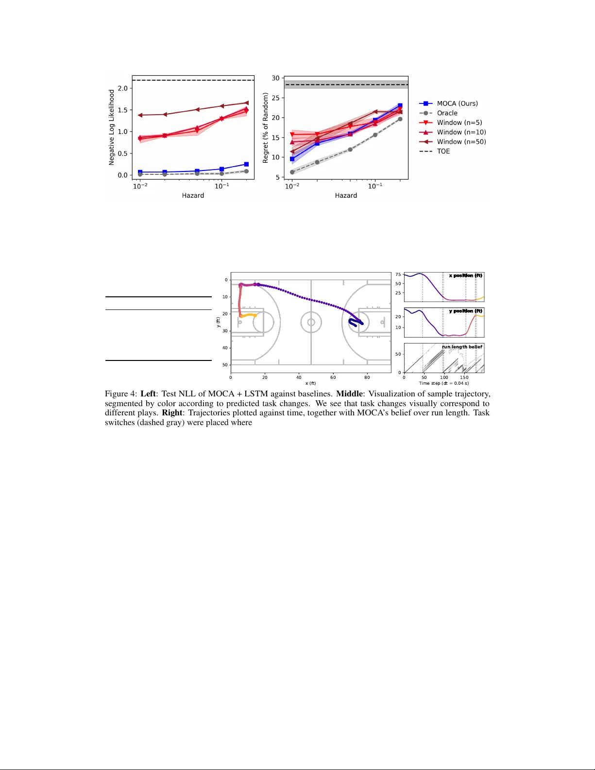
Continuous Meta-Lear ning without T asks James Harrison, A poorv a Sharma, Chelsea Finn, Mar co Pa vone Stanford Univ ersity , Stanford, CA {jharrison, apoorva, cbfinn, pavone}@stanford.edu Abstract Meta-learning is a promising strategy for learning to efﬁciently learn using data gathered from a distrib ution of tasks. Howe v er , the meta-learning literature thus far has focused on the task se gmented setting, where at train-time, of ﬂine data is assumed to be split according to the underlying task, and at test-time, the algorithms are optimized to learn in a single task. In this work, we enable the application of generic meta-learning algorithms to settings where this task segmentation is unav ailable, such as continual online learning with unse gmented time series data. W e present meta-learning via online changepoint analysis (MOCA), an approach which augments a meta-learning algorithm with a differentiable Bayesian change- point detection scheme. The framework allo ws both training and testing directly on time series data without se gmenting it into discrete tasks. W e demonstrate the utility of this approach on three nonlinear meta-regression benchmarks as well as two meta-image-classiﬁcation benchmarks. 1 Introduction Meta-learning methods ha ve recently sho wn promise as an ef fective strate gy for enabling efﬁcient few-shot learning in complex domains from image classiﬁcation to nonlinear regression [ 10 , 40 ]. These methods le verage an ofﬂine meta-learning phase, in which data from a collection of learning tasks is used to learn priors and update rules for more efﬁcient learning on ne w related tasks. Meta-learning algorithms hav e thus far solely focused on settings with task se gmentation , where the learning agent knows when the latent task changes. At meta-train time, these algorithms assume access to a meta-dataset of datasets from indi vidual tasks, and at meta-test time, the learner is ev aluated on a single task. Howe ver , there are many applications where task segmentation is unav ailable, which hav e been under-addressed in the meta-learning literature. For e xample, environmental f actors may change during a robot’ s deployment, and these changes may not be directly observed. Furthermore, crafting a meta-dataset from an existing stream of experience may require a difﬁcult or expensi ve process of detecting switches in the task. In this work, we aim to enable meta-learning in task-unse gmented settings, operating directly on time series data in which the latent task undergoes discrete, unobserved switches, rather than requiring a pre-segmented meta-dataset. Equiv alently , from the perspectiv e of online learning, we wish to optimize an online learning algorithm using past data sequences to perform well in a sequential prediction setting wherein the underlying data generating process (i.e. the task) may vary with time. Contributions. Our primary contrib ution is an algorithmic framework for task unsegmented meta- learning which we refer to as meta-learning via online changepoint analysis (MOCA). MOCA wraps arbitrary meta-learning algorithms in a differentiable Bayesian changepoint estimation scheme, enabling their application to problems that require continual learning on time series data. By backpropagating through the changepoint estimation framew ork, MOCA learns both a rapidly adaptiv e underlying predictiv e model (the meta-learning model), as well as an ef fectiv e changepoint detection algorithm, optimized to work together . MOCA is a generic frame work which works with 34th Conference on Neural Information Processing Systems (NeurIPS 2020), V ancouv er, Canada. many existing meta-learning algorithms. W e demonstrate MOCA on both regression and classiﬁcation settings with unobserved task switches. 2 Problem Statement Our goal is to enable meta-learning in the general setting of sequential prediction, in which we observe a sequence of inputs x t and their corresponding labels y t . In this setting, the learning agent makes probabilistic predictions o ver the labels, le veraging past observ ations: p θ ( ˆ y t | x 1: t , y 1: t − 1 ) , where θ are the parameters of the learning agent. W e assume the data are drawn from an underlying generativ e model; thus, given a training sequence from this model D train = ( x 1: N , y 1: N ) , we can optimize θ to perform well on another sample sequence from the same model at test time. W e assume data is drawn according to a latent (unobserved) task T t , that is x t , y t ∼ p ( x , y | T t ) . Further , we assume that ev ery so often, the task switches to a new task sampled from some distrib ution p ( T ) . At each timestep, the task changes with probability λ , which we refer to as the hazard rate. W e ev aluate the learning algorithm in terms of a log likelihood, leading to the follo wing objective: min θ E " ∞ X t =1 − log p θ ( y t | x 1: t , y 1: t − 1 ) # (1) subj. to x t , y t ∼ p ( x , y | T t ) , T t =  T t − 1 w .p. 1 − λ T t, new w .p. λ , T 1 ∼ p ( T ) , T t, new ∼ p ( T ) Giv en D train , we can approximate this expectation and thus learn θ at train time. Note that just as in standard meta-learning, we lev erage data drawn from a di verse collection of tasks in order to optimize a learning agent to do well on ne w tasks at test time. Howe ver , there are three key dif ferences from standard meta-learning: • The learning agent continually adapts as it is e valuated on its predictions, rather than only adapting on k labeled examples, as is common in fe w-shot learning. • At train time, data is unsegmented , i.e. not grouped by the latent task T . • Similarly , at test time, the task changes with time, so the agent must infer which past data are drawn from the current task when making predictions. Thus, the setting we consider here can be considered a generalization of the standard meta-learning setting, relaxing the requirement of task segmentation at train and test time. Both our problem setting and an illustration of the MOCA algorithm are presented in Fig. 1. 3 Preliminaries Meta-Learning . The core idea of meta-learning is to directly optimize the few-shot learning performance of a machine learning model over a distribution of learning tasks, such that this learning performance generalizes to other tasks from this distribution. A meta-learning method consists of two phases: meta-training and online adaptation. Let θ be the parameters of this model learned in meta-training. During online adaptation, the model uses context data D t = ( x 1: t , y 1: t ) from within one task to compute statistics η t = f θ ( D t ) , where f is a function parameterized by θ . For example, in MAML [ 10 ], the statistics are the neural network weights after gradient updates computed using D t . For recurrent netw ork-based meta-learning algorithms, these statistics correspond to the hidden state of the network. For a simple nearest-neighbors model, η may simply be the context data. The model then performs predictions by using these statistics to deﬁne a conditional distribution on y giv en new inputs x , which we write y | x , D t ∼ p θ ( y | x , η t ) . Adopting a Bayesian perspectiv e, we refer to p θ ( y | x , η t ) as the posterior predictiv e distribution. The performance of this model on this task can be ev aluated through the log-likelihood of task data under this posterior predictiv e distribution L ( D t , θ ) = E x , y ∼ p ( · , ·|T i ) [ − log p θ ( y | x , f θ ( D t ))] . Meta-learning algorithms, broadly , aim to optimize the parameters θ such that the model performs well across a distribution of tasks, min θ E T i ∼ p ( T ) [ E D t ∼T i [ L ( D t , θ )]] . Across most meta-learning algorithms, both the update rule f θ ( · ) and the prediction function are chosen to be differentiable operations, such that the parameters can be optimized via stochastic gradient descent. Giv en a dataset 2 Figure 1: An illustration of a simpliﬁed version of our problem setting and of the MOCA algorithm. An agent sequentially observes an input x (e.g, an image), makes a probabilistic prediction, and recei ves the true label y (here, class 1 or 2). An unobserv ed change in the task (a “changepoint”) results in a change in the generativ e model of x and/or y . In the abov e image, the images corresponding to label 1 switch from sailboats to school buses, while the images corresponding to label 2 switch from sloths to geese. MOCA recursively estimates the time since the last changepoint, and conditions an underlying meta-learning model only on data that is rele vant to the current task to optimize its predictions. pre-segmented into groups of data from individual tasks, standard meta-learning algorithms can estimate this expectation by ﬁrst sampling a group for which T is ﬁxed, then treating one part as context data D t , and sampling from the remainder to obtain test points from the same task. While this strategy is ef fectiv e for few-shot learning, it fails for settings like sequential prediction, where the latent task may change over time and segmenting data by task is dif ﬁcult. Our goal is to bring meta-learning tools to such settings. Bayesian Online Changepoint Detection . T o enable meta-learning without task segmentation, we build upon Bayesian online changepoint detection [ 1 ], an approach for detecting discrete changes in a data stream (i.e. task switches), originally presented in an unconditional density estimation context. BOCPD operates by maintaining a belief distribution over run lengths , i.e. how many past data points were generated under the current task. A run length r t = 0 implies that the task has switched at time t , and so the current datapoint y t was drawn from a new task T 0 ∼ p ( T ) . W e denote this belief distribution at time t as b t ( r t ) = p ( r t | y 1: t − 1 ) . W e can reason about the overall posterior predicti ve by mar ginalizing over the run length r t according to b t ( r t ) , p ( y t | y 1: t − 1 ) = P t − 1 τ =0 p ( y t | y 1: t − 1 , r t = τ ) b t ( τ ) , Gi ven r t = τ , we kno w the past τ data points all correspond to the current task, so p ( y t | y 1: t − 1 , r t = τ ) can be computed as the posterior predictiv e of an underlying predictive model (UPM), conditioning on the past τ data points. BOCPD recursi vely computes posterior predictive densities using this UPM for each value of r t ∈ { 0 , . . . , t − 1 } , and then e valuates new datapoints y t +1 under these posterior predictiv e densities to update the belief distribution b ( r t ) . In this work, we extend these techniques to conditional density estimation, deriving update rules which use meta-learning models as the UPM. 4 Meta-Learning via Online Changepoint Analysis W e now present MOCA 1 , which enables meta-learning in settings without task segmentation, both at train and test time. In the following subsections, we ﬁrst e xtend BOCPD to deri ve a recursive Bayesian ﬁltering algorithm for run length, lev eraging a base meta-learning algorithm as the underlying predicti ve model (UPM). W e then outline ho w the full framework allo ws both training and ev aluating meta-learning models on time series without task segmentation. 4.1 Bayesian T ask Duration Estimation As in BOCPD, MOCA maintains a belief over possible run lengths r t . Throughout this paper , we use b t to refer to the belief befor e observing data at that timestep, ( x t , y t ) . Note that b t is a discrete distribution with support over r t ∈ { 0 , ..., t − 1 } . MOCA also maintains a version of the base meta-learning algorithm’ s posterior parameters η for ev ery possible run length. W e write η t [ r ] to refer to the posterior parameters produced by the meta-learning algorithm after adapting to the past r 1 Code is av ailable at https://github.com/StanfordASL/moca 3 Algorithm 1 Meta-Learning via Online Changepoint Analysis Require: Training data x 1: n , y 1: n , number of training iterations N , initial model parameters θ 1: for i = 1 to N do 2: Sample training batch x 1: T , y 1: T from the full timeseries. 3: Initialize run length belief b 1 ( r 1 = 0) = 1 , posterior statistics η 0 [ r = 0] according to θ 4: for t = 1 to T do 5: Observe x t , compute b t ( r t | x t ) via (2) 6: Predict p θ ( ˆ y t | x 1: t , y 1: t − 1 ) via (5) 7: Observe y t and incur NLL loss ` t = − log p θ ( y t | x 1: t , y 1: t − 1 ) 8: Compute updated posteriors η t [ r t ] for all r t via (6) 9: Compute b t ( r t | x t , y t ) via (3) 10: Compute updated belief ov er run length b t +1 via (4) 11: end for 12: Compute ∇ θ P k + T t = k ` t and take gradient descent step to update θ 13: end for datapoints, ( x t − r +1: t , y t − r +1: t ) . Giv en this collection of posteriors, we can compute the likelihood of observing data giv en the run length r . This allows us to apply rules from Bayesian ﬁltering to update the run length belief in closed form. These updates in volve three steps: If the base meta-learning algorithm maintains a posterior distribution of inputs p θ ( x t | η t − 1 ) , then MOCA can update the belief b t directly after observing x t , as follows b t ( r t | x t ) := p ( r t | x 1: t , y 1: t − 1 ) ∝ p θ ( x t | η t − 1 [ r t ]) b t ( r t ) (2) which can be normalized by summing ov er the ﬁnite support of b t . This step relies on maintaining a generativ e model of the input variable, which is atypical for most regression models and is not done for discriminativ e classiﬁcation models. While this ﬁltering step is optional, it allows MOCA to detect task switches based on a changes in the input distribution when possible. Next, upon observing the label y t , we can use the base meta-learning algorithm’ s conditional posterior predictiv e p θ ( y t | x t , η t − 1 ) to again update the belief ov er run length: b t ( r t | x t , y t ) := p ( r t | x 1: t , y 1: t ) ∝ p θ ( y t | x t , η t − 1 [ r t ]) b t ( r t | x t ) , (3) which can similarly be normalized. Finally , to push the run length belief forward in time, we note that we assume that the task switches with probability λ at ev ery timestep, and so the task remains ﬁxed with probability 1 − λ . This yields the update b t +1 ( r t +1 = k ) =  λ if k = 0 (1 − λ ) b t ( r t = k − 1 | x t , y t ) if k > 0 . (4) For more details on the deri vation of these updates, we refer the reader to Appendix A. 4.2 Meta Learning without T ask Segmentation By taking a Bayesian ﬁltering approach to changepoint detection, we avoid hard assignments of changepoints and instead perform a soft selection over run lengths. In this way , MOCA is able to backpropagate through the changepoint detection and directly optimize the underlying predictiv e model, which may be any meta-learning model that admits a probabilistic interpretation. MOCA processes a time series sequentially . W e initialize b 1 ( r 1 = 0) = 1 , and initialize the posterior statistics for η 0 [ r 1 = 0] as speciﬁed by the parameters θ of the meta learning algorithm. Then, at timestep t , we ﬁrst observe inputs x t and compute b t ( r t | x t ) according to (2) . Next, we marginalize to make a probabilistic prediction for the label, p θ ( ˆ y t | x 1: t , y 1: t − 1 ) equal to t − 1 X r t =0 b t ( r t | x t ) p θ ( ˆ y t | x t , η t − 1 [ r t ]) (5) W e then observe the label y t and incur the corresponding loss. W e can also use the label both to compute b t ( r t | x t , y t ) according to (3) , as well as to update the posterior statistics for all the run 4 lengths using the labeled example. Many meta-learning algorithms admit a recursiv e update rule which allows these parameters to be computed ef ﬁciently using the past values of η , η t [ r ] = h ( x t , y t , η t − 1 [ r − 1]) ∀ r = 1 , . . . , t. (6) While MOCA could work without such a recursi ve update rule, this would require storing data online and running the non-recursi ve posterior computation η t = f θ (( x t − r t +1: t , y t − r t +1: t )) for e very r t , which in volv es t operations using datasets of sizes from 0 to t , and thus can be an O ( t 2 ) operation. In contrast, the recursiv e updates in volve t operations in volving just the latest datapoint, yielding O ( t ) complexity . Finally , we propagate the belief over run length forward in time to obtain b t ( r t +1 ) to be ready to process the next data point in the timeseries. Since all these operations are differentiable, giv en a training time series in which there are task switches D train , we can run this procedure, sum the negati ve log likelihood (NLL) losses incurred at each step, and use backpropagation within a standard automatic differentiation framework to optimize the parameters of the base learning algorithm, θ . Algorithm 1 outlines this training procedure. In practice, we sample shorter time series of length T from the training data to ease computational requirements during training; we discuss implications of this in Appendix D. If av ailable, a user can input various le vels of kno wledge on task segmentation by manually updating b ( r t ) at any time; further details and empirical validation of this task semi-segmented use case are also provided in Appendix D 4.3 Making your MOCA: Model Instantiations Thus far , we hav e presented MOCA at an abstract lev el, highlighting the fact that it can be used with any meta-learning model that admits the probabilistic interpretation as the UPM. Practically , as MOCA maintains sev eral copies of the posterior statistics η , meta-learning algorithms with lower -dimensional posterior statistics which admit recursive updates yield better computational efﬁcienc y . W ith this in mind, for our e xperiments we implemented MOCA using a v ariety of base meta-learners: an LSTM-based meta-learning approach [ 21 ], as well as meta-learning algorithms based on Bayesian modeling which e xploit conjugate prior/likelihood models allo wing for closed- form recursiv e posterior updates, speciﬁcally ALPaCA [ 16 ] for regression and a novel algorithm in a similar vein which we call PCOC, for probabilistic clustering for online classiﬁcation, for classiﬁcation. Further details on all methods are provided in Appendix B. LSTM Meta-learner . The LSTM meta-learning approach encodes the information in the observ ed samples using hidden state h t of an LSTM [ 20 ], and subsequently uses this hidden state to make predictions. Speciﬁcally , we follow the architecture proposed in [ 21 ], wherein an encoding of the current input z t = φ ( x t , w ) as well as the pre vious label y t − 1 are fed as input to the LSTM cell to update the hidden state h t and cell state c t . For regression, the mean and variance of a Gaussian posterior predictiv e distribution are output as a function of the hidden state and encoded input [ µ, Σ] = f ( h t , z t ; w f ) . The function f is a feedforward network in both cases, with weights w f . W ithin the MOCA framework, the posterior statistics for this model are η t = { h t , c t , y t } . ALPaCA: Bayesian Meta-Lear ning for Regr ession. ALPaCA is a meta-learning approach which performs Bayesian linear regression in a learned feature space, such that y | x ∼ N ( K T φ ( x , w ) , Σ  ) where φ ( x , w ) is a feed-forward neural network with weights w mapping inputs x to a n φ - dimensional feature space. ALP aCA maintains a matrix-normal distribution over K , and thus results in a matrix-normal posterior distribution o ver K . This posterior inference may be performed exactly , and computed recursively . The matrix-normal distribution on the last layer results in a Gaussian posterior predicti ve density . Note that, as is typical in regression, ALP aCA only models the conditional density p ( y | x ) , and assumes that p ( x ) is independent of the underlying task. The algorithm parameters θ are the prior on the last layer, as well as the weights w of the neural network feature network φ . The posterior statistics η encode the mean and variance of the Gaussian posterior distribution on the last layer weights. PCOC: Bayesian Meta-Learning f or Classiﬁcation. In the classiﬁcation setting, one can obtain a similar Bayesian meta-learning algorithm by performing Gaussian discriminant analysis in a learned feature space. W e refer to this novel approach to meta-learning for classiﬁcation as probabilistic clustering for online classiﬁcation (PCOC). Labeled input/class pairs ( x t , y t ) are processed by encoding the input through an embedding network z t = φ ( x t ; w ) , and performing Bayesian density estimation in this feature space for ev ery class. Speciﬁcally , we assume a Categorical-Gaussian generativ e model in this embedding space, and impose the conjugate Dirichlet prior o ver the class 5 0 20 40 60 80 Time step 0 20 40 Run length t=20 t=67 Figure 2: MOCA with ALPaCA on the sinusoid re gression problem. Left: The belief ov er run length versus time. The intensity of each point in the plot corresponds to the belief in run length at the associated time. The red lines sho w the true changepoints. Middle, Right: V isualizations of the posterior predicti ve density at the times marked by blue lines in the left ﬁgure. The red line denotes the current function (task), and red points denote data from the current task. Green points denote data from previous tasks, where more faint points are older . By reasoning about task run-length, MOCA ﬁts the current sinusoid while avoiding ne gative transfer from past data, and resets to prior predictions when tasks switch. probabilities and a Gaussian prior o ver the mean for each class. This ensures the posterior remains Dirichlet-Gaussian, whose parameters can be updated recursively . The posterior parameters η for this algorithm are the mean and cov ariance of the posterior distribution on each class mean, as well as the counts of observations per class. The learner parameters θ are the weights of the encoding network w , the prior parameters, and the cov ariance assumed for the observation noise. PCOC can be thought of a Bayesian analogue of prototypical networks [40]. 5 Related W ork Online Learning, Continuous Lear ning, and Concept Drift Adaptation. A substantial literature exists on online, continual and lifelong learning [ 18 , 6 ]. These ﬁelds all consider learning within a streaming series of tasks, wherein it is desirable to re-use information from pre vious tasks while av oiding negati ve transfer [ 12 , 42 ]. T ypically , continual learning assumes access to task segmentation information, whereas online learning does not [ 3 ]. Regularization approaches [ 26 , 18 , 28 ] hav e been sho wn to be an effecti ve method for a voiding for getting in continual learning. By augmenting the loss function for a ne w task with a penalty for de viation from the parameters learned for pre vious tasks, the regularizing ef fects of a prior are mimicked; in contrast we explicitly learn a prior ov er task weights that is meta-trained to be rapidly adaptiv e. Thus, MOCA is capable of av oiding substantial negati ve transfer by detecting task change, and rapidly adapting to ne w tasks. [ 3 ] loosen the assumption of task segmentation in continual learning and operate in a similar setting to that addressed herein, b ut they aim to optimize one model for all tasks simultaneously; in contrast, our work takes a meta-learning approach and aims to optimize a learning algorithm to quickly adapt to changing tasks. Meta-Learning f or Continuous and Online Learning. In response to the slow adaption of contin- ual learning algorithms, there has been substantial interest in applying ideas from meta-learning to continual learning to enable rapid adaptation to ne w tasks. T o handle streaming data, sev eral works [ 31 , 19 ] use a sliding window approach, wherein a ﬁx ed amount of past data is used to condition the meta-learned model. As this window length is not reacti ve to task change, these models risk suf fering from negati ve transfer . Indeed, MOCA may be interpreted as sliding window model, that acti vely infers the optimal window length. [ 32 ] and [ 24 ] aim to detect task changes online by combining mean estimation of the labels with MAML. Ho wever , these models are less expressi ve than MOCA (which maintains a full Bayesian posterior), and require task segmentation as test time. [ 36 ] employ gradient-based meta-learning to improv e transfer between tasks in continual learning; in contrast MOCA works with any meta-learning algorithm. Empirical Bayes f or Changepoint Models. Follo w-on work to BOCPD [ 1 ] and the similar simulta- neous work of [ 9 ] has considered applying empirical Bayes to optimize the underlying predictiv e model, a similar problem to that addressed herein. In particular , [ 33 ] de velop a forward-backward algorithm that allows closed-form max likelihood estimation of the prior for simple distributions via EM. [ 43 ] deri ve general-purpose gradients for h yperparameter optimization within the BOCPD model. MOCA pairs these ideas with neural network meta-learning models, and thus can le verage recent advances in automatic dif ferentiation for gradient computation. 6 Figure 3: Performance of MOCA with ALPaCA versus baselines in sinusoid regression ( left ) and the switching wheel contextual bandit problem ( right ). In the bandit problem, we ev aluate performance as the regret of the model (compared to an optimal decision maker with perfect knowledge of switch times) as a percentage of the regret of the random agent, follo wing previous w ork [ 37 ]. In both problems, lo wer is better . Conﬁdence interv als in this ﬁgure and throughout are 95%. Model T est NLL TOE 0 . 889 ± 0 . 073 SW5 − 3 . 032 ± 0 . 058 SW10 − 3 . 049 ± 0 . 054 SW50 − 3 . 061 ± 0 . 054 COE − 3 . 044 ± 0 . 059 MOCA − 3 . 291 ± 0 . 074 0 20 40 60 80 x (ft) 0 10 20 30 40 50 y (ft) 25 50 75 x position (ft) x position (ft) x position (ft) x position (ft) x position (ft) x position (ft) x position (ft) 10 20 y position (ft) y position (ft) y position (ft) y position (ft) y position (ft) y position (ft) y position (ft) 0 50 100 150 Time step (dt = 0.04 s) 0 50 run length belief Figure 4: Left : T est NLL of MOCA + LSTM against baselines. Middle : V isualization of sample trajectory , segmented by color according to predicted task changes. W e see that task changes visually correspond to different plays. Right : T rajectories plotted against time, together with MOCA ’ s belief over run length. T ask switches (dashed gray) were placed where the MAP run length drops to a value less than 5. 6 Experimental Results W e in vestigate the performance of MOCA in ﬁv e problem settings: three in regression and two in classiﬁcation. Our primary goal is to characterize how ef fectiv ely MOCA can enable meta-learning algorithms to perform without access to task segmentation. W e compare against baseline sliding window models, which again use the same meta-learning algorithm, but always condition on the last n data points, for n ∈ { 5 , 10 , 50 } . These baselines are a competitive approach to learning in time-v arying data streams [ 13 ] and ha ve been applied meta-learning in time-v arying settings [ 31 ]. W e also compare to a “train on e verything” model, which only learns a prior and does not adapt online, corresponding to a standard supervised learning approach. Finally , where possible, we compare MOCA against an “oracle” model that uses the same base meta-learning algorithm, but has access to exact task se gmentation at train and test time, to explicitly characterize the utility of task se gmentation. Due to space constraints, this section contains only core numerical results for each problem setting; further experiments and ablations are presented in the appendix. W e ﬁnd by explicitly reasoning about task run-length, MOCA is able to outperform baselines across all the domains with a variety of base meta-learning algorithms and provide interpretable estimates of task-switches at test time. Sinusoid Regression . T o characterize MOCA in the regression setting, we inv estigate the perfor- mance on a switching sinusoid problem adapted from [10], in which a task change corresponds to a re-sampled sinusoid phase and amplitude. Qualitativ e results are visualized for the sinusoid in Fig. 2. In this problem we pair MOCA with ALPaCA as it outperforms LSTM-based meta-learners. MOCA is capable of accurate and calibrated posterior inference with only a handful of data points, and is capable of rapidly identifying task change. T ypically , it identiﬁes task change in one timestep, unless the datapoint happens to ha ve high lik elihood under the previous task as in Fig. 2d. Performance of MOCA against baselines is presented in Fig. 3 for all problem domains. For sinusoid (left), MOCA 7 Figure 5: Performance of MOCA with PCOC on rainbow MNIST ( left ) and miniImageNet ( right ). In both problems, higher is better . achiev es performance close to the oracle model and substantially outperforms the sliding window approaches for all hazard rates. Wheel Bandit . Bandit problems hav e seen recent highly fruitful application of meta-learning algorithms [ 4 , 45 , 15 ]. W e inv estigate the performance of MOCA (paired with ALPaCA) in the switching bandit problem, in which the rew ard function of the bandit undergoes discrete changes [ 14 , 17 , 30 ]. W e extend the wheel bandit problem [ 37 ], a common benchmark for meta-learning algorithms [ 15 , 34 ]. Details of the full bandit problem are provided in the appendix. In this problem, changepoint identiﬁcation is difﬁcult, as only a small subset of states contains information about whether the rew ard function has changes. Follo wing [ 30 ], we use Thompson sampling for action selection. W e use the notion of regret deﬁned in [ 14 ], in which the chosen action is compared to the action with the best mean rew ard at each time, with perfect knowledge of switches. As shown in [ 14 ], the sliding window baselines have strong theoretical guarantees on regret, as well as good empirical performance. Performance is plotted in Fig. 3. MOCA outperforms baselines for lower hazard rates. Detecting task switches requires observing a state close to the (changing) high-re ward boundary , and at high hazard rates, the rapid task changes make identiﬁcation of changepoints difﬁcult, and we see that MOCA performance matches all the sliding windows in this re gime. NB A Player Movement . T o test MOCA on a real-w orld data with an unobserved switching latent task, we test it on predicting the mo vement of NB A players, whose intent may switch o ver time, from, e.g., running to wards a position on the three-point line, to moving inside the ke y to recover a rebound. This changing latent state has made it a common benchmark for recurrent predictive models [ 22 , 29 ]. In our experiments, the input x is an indi vidual player’ s current position on the court ( x t , y t ) , and the label y t = x t +1 − x t is the step the player takes at that time. For this problem, we pair MOCA with the LSTM meta-learner , since recurrent models are well suited to this task and we sa w better performance relativ e to ALPaCA. W e add a “condition on ev erything” (COE) baseline which updates a single set of posterior statistics η using all a vailable data, as the LSTM can theoretically learn to only consider relev ant data. Nevertheless, we ﬁnd that that MOCA’ s explicit reasoning over task length yields better performance over COE and other baselines, as shown in Fig. 4. While true task segmentation is una vailable for this data, we see in the ﬁgure that MOCA’ s predictions of task changes correspond intuitiv ely to changes in the player’ s intent. Rainbow MNIST . In the classiﬁcation setting, we apply MOCA with PCOC to the Rainbo w MNIST dataset of [ 11 ]. In this dataset, MNIST digits ha ve been perturbed via a color change, rotation, and scaling; each task corresponds to a unique combination of these transformations. Relative to baselines, MOCA approaches oracle performance for lo w hazard rates, due in part to the fact that task change can usually be detected prior to prediction via a change in digit color . Sev en colors were used, so with probability 6 / 7 , MOCA has a strong indicator of task change before observing the image class. miniImageNet . Finally , we in vestigate the performance of MOCA with PCOC on the miniImageNet benchmark task [ 44 ]. This dataset consists of 100 ImageNet categories [ 7 ], each with 600 RGB images of resolution 84 × 84 . In our continual learning setting, we associate each class with a semantic label that is consistent between tasks. As ﬁve-w ay classiﬁcation is standard for miniImageNet [ 44 , 40 ], we split the miniImageNet dataset in to ﬁ ve approximately balanced “super-classes." F or example, 8 one super-class is dog breeds, while another is food, kitchen and clothing items; details are provided in the appendix. Each ne w task corresponds to resampling a particular class from each super -class from which to draw inputs x ; the labels y remain the ﬁve super-classes, enabling knowledge re- use between classes. This corresponds to a continual learning scenario in which each super-class experiences distributional shift over time. Fig. 5 shows that MOCA outperforms baselines for all hazard rates. 7 Discussion and Conclusions Future W ork. In this work, we address the case in which tasks are sampled i.i.d. from a (typically continuous) distribution, and thus kno wledge re-use adds marginal v alue. Ho wev er , many domains may hav e tasks that can reoccur , or temporal dynamics to task ev olution and thus data efﬁcienc y may be improv ed by re-using information for pre vious tasks. Previous work [ 32 , 24 , 27 ] has addressed the case in which tasks reoccur in both meta-learning and the BOCPD framew ork, and thus knowledge (in the form of a posterior estimate) may be re-used. Broadly , moving beyond the assumption of i.i.d. tasks to tasks having associated dynamics [2] represents a promising future direction. Conclusions. MOCA enables the application of existing meta-learning algorithms to problems without task segmentation, such as the problem setting of continual learning. W e ﬁnd that by lev eraging a Bayesian perspectiv e on meta-learning algorithms and augmenting these algorithms with a Bayesian changepoint detection scheme to automatically detect task switches within time series, we can achie ve similar predictiv e performance when compared to the standard task-segmented meta-learning setting, without the often prohibitiv e requirement of supervised task segmentation. Funding Disclosure and Ackno wledgments James Harrison was supported in part by the Stanford Graduate Fello wship and the National Sciences and Engineering Research Council of Canada (NSERC). The authors were partially supported by an Early Stage Innovations grant from NASA ’ s Space T echnology Research Grants Program, and by D ARP A, Assured Autonomy program. The authors wish to thank Matteo Zallio for help in the design of ﬁgures. Broader Impact Our work provides a method to e xtend meta-learning algorithms beyond the task-se gmented case, to the time series series domain. Equiv alently , our work extends core methods in changepoint detection, enabling the use of highly expressiv e predicti ve models via empirical Bayes. This work has the potential to extend the domain of applicability of both of these methods. Standard meta-learning relies on a collection of datasets, each corresponding to discrete tasks. A natural question is ho w such datasets are constructed; in many cases, these datasets rely on se gmentation of time series data by experts. Thus, our work has the potential to make meta-learning algorithms applicable to problems that, pre viously , would hav e been too expensi ve or impossible to segment. Moreover , our work has the potential to impro ve the applicability of changepoint detection methods to difﬁcult time series forecasting problems. While MOCA has the potential to expand the domain of problems addressable via meta-learning, this has the effect of amplifying the risks associated with these methods. Meta-learning enables efﬁcient learning for individual members of a population via leveraging empirical priors. There are clear risks in few-shot learning generally: for example, ef ﬁcient facial recognition from a handful of images has clear negati ve implications for pri vac y . Moreover , while there is promising initial work on f airness for meta-learning [ 39 ], we belie ve considerable future research is required to understand the degree to which meta-learning algorithms increase undesirable bias or decrease fairness. While it is plausible that ﬁne-tuning to the indi vidual results in reduced bias, there are potential unforeseen risks associated with the adaptation process, and future research should address how bias is potentially introduced in this process. Relativ e to decision making rules that are ﬁxed across a population, algorithms which ﬁne-tune decision making to the indi vidual present unique challenges in analyzing fairness. Further research is required to ensure that the adaptiv e learning enabled by algorithms such as MOCA do not lead to unfair outcomes. 9 References [1] Ryan Prescott Adams and David JC MacKay . Bayesian online changepoint detection. arXiv:0710.3742 , 2007. [2] Maruan Al-Shediv at, Trapit Bansal, Y uri Burda, Ilya Sutskev er , Igor Mordatch, and Pieter Abbeel. Continuous adaptation via meta-learning in nonstationary and competiti ve environments. International Confer ence on Learning Representations (ICLR) , 2018. [3] Rahaf Aljundi, Klaas Kelchtermans, and T inne Tuytelaars. T ask-free continual learning. Com- puter V ision and P attern Recognition (CVPR) , 2019. [4] Leonardo Cella, Alessandro Lazaric, and Massimiliano Pontil. Meta-learning with stochastic linear bandits. , 2020. [5] W ei-Y u Chen, Y en-Cheng Liu, Zsolt Kira, Y u-Chiang Frank W ang, and Jia-Bin Huang. A closer look at few-shot classiﬁcation. International Confer ence on Learning Representations (ICLR) , 2019. [6] Zhiyuan Chen and Bing Liu. Lifelong machine learning. Synthesis Lectures on Artiﬁcial Intelligence and Machine Learning , 2016. [7] J. Deng, W . Dong, R. Socher , L.-J. Li, K. Li, and L. Fei-Fei. ImageNet: A Large-Scale Hierarchical Image Database. Computer V ision and P attern Recognition (CVPR) , 2009. [8] Bradley Efron and Carl Morris. Stein’ s estimation rule and its competitors—an empirical Bayes approach. Journal of the American Statistical Association , 1973. [9] Paul Fearnhead and Zhen Liu. On-line inference for multiple changepoint problems. Journal of the Royal Statistical Society: Series B (Statistical Methodology) , 2007. [10] Chelsea Finn, Pieter Abbeel, and Sergey Le vine. Model-agnostic meta-learning for fast adapta- tion of deep networks. International Conference on Mac hine Learning (ICML) , 2017. [11] Chelsea Finn, Ara vind Rajeswaran, Sham Kakade, and Ser gey Levine. Online meta-learning. International Confer ence on Machine Learning (ICML) , 2019. [12] Robert M French. Catastrophic forgetting in connectionist networks. T r ends in cognitive sciences , 1999. [13] João Gama, Indr ˙ e Žliobait ˙ e, Albert Bifet, Mykola Pechenizkiy , and Abdelhamid Bouchachia. A surve y on concept drift adaptation. ACM computing surve ys (CSUR) , 2014. [14] Aurélien Garivier and Eric Moulines. On upper-conﬁdence bound policies for switching bandit problems. International Confer ence on Algorithmic Learning Theory , 2011. [15] Marta Garnelo, Jonathan Schwarz, Dan Rosenbaum, Fabio V iola, Danilo J. Rezende, S.M. Ali Eslami, and Y ee Whye T eh. Neural processes. International Conference on Mac hine Learning (ICML) , 2018. [16] James Harrison, Apoorva Sharma, and Marco P avone. Meta-learning priors for efﬁcient online Bayesian regression. W orkshop on the Algorithmic F oundations of Robotics (W AFR) , 2018. [17] Cédric Hartland, Nicolas Baskiotis, Sylv ain Gelly , Michèle Sebag, and Oli vier T eytaud. Change point detection and meta-bandits for online learning in dynamic en vironments. 2007. [18] Elad Hazan. Introduction to online conv ex optimization. F oundations and T r ends ® in Opti- mization , 2016. [19] Xu He, Jakub Sygnowski, Ale xandre Galashov , Andrei A Rusu, Y ee Whye T eh, and Razvan Pascanu. T ask agnostic continual learning via meta learning. arXiv pr eprint arXiv:1906.05201 , 2019. [20] Sepp Hochreiter and Jürgen Schmidhuber . Long short-term memory . Neur al computation , 1997. [21] Sepp Hochreiter, A Stev en Y ounger, and Peter R Conwell. Learning to learn using gradient descent. International Confer ence on Artiﬁcial Neural Networks (ICANN , 2001. [22] Boris Ivano vic, Edward Schmerling, Karen Leung, and Marco Pav one. Generative modeling of multimodal multi-human beha vior . IEEE International Confer ence on Intelligent Robots and Systems (IR OS) , 2018. [23] Khurram Ja ved and Martha White. Meta-learning representations for continual learning. Neural Information Pr ocessing Systems (NeurIPS) , 2019. 10 [24] Ghassen Jerfel, Erin Grant, Thomas L Grif ﬁths, and Katherine Heller . Online gradient-based mixtures for transfer modulation in meta-learning. Neural Information Pr ocessing Systems (NeurIPS) , 2019. [25] Diederik P Kingma and Jimmy Ba. Adam: A method for stochastic optimization. International Confer ence on Learning Representations (ICLR) , 2015. [26] James Kirkpatrick, Razv an Pascanu, Neil Rabinowitz, Joel V eness, Guillaume Desjardins, Andrei A Rusu, Kieran Milan, John Quan, T iago Ramalho, Agnieszka Grabska-Barwinska, et al. Overcoming catastrophic for getting in neural networks. Pr oceedings of the National Academy of Sciences (PN AS) , 2017. [27] Jeremias Knoblauch and Theodoros Damoulas. Spatio-temporal bayesian on-line changepoint detection with model selection. International Confer ence on Machine Learning (ICML) , 2018. [28] Zhizhong Li and Derek Hoiem. Learning without forgetting. IEEE T ransactions on P attern Analysis & Machine Intelligence , 2017. [29] Scott W Linderman, Andrew C Miller , Ryan P Adams, David M Blei, Liam Paninski, and Matthew J Johnson. Recurrent switching linear dynamical systems. , 2016. [30] Joseph Mellor and Jonathan Shapiro. Thompson sampling in switching en vironments with bayesian online change detection. Artiﬁcial Intelligence and Statistics (AIST ATS) , 2013. [31] Anusha Nagabandi, Ignasi Clav era, Simin Liu, Ronald S Fearing, Pieter Abbeel, Sergey Le vine, and Chelsea Finn. Learning to adapt in dynamic, real-world environments through meta- reinforcement learning. International Confer ence on Learning Representations (ICLR) , 2019. [32] Anusha Nagabandi, Chelsea Finn, and Serge y Levine. Deep online learning via meta-learning: Continual adaptation for model-based RL. International Confer ence on Learning Representa- tions (ICLR) , 2019. [33] Ulrich Paquet. Empirical Bayesian change point detection. Graphical Models , 2007. [34] Sachin Ravi and Ale x Beatson. Amortized bayesian meta-learning. International Confer ence on Learning Repr esentations (ICLR) , 2018. [35] Mengye Ren, Eleni Triantaﬁllou, Sachin Ravi, Jake Snell, Ke vin Swersky , Joshua B T enen- baum, Hugo Larochelle, and Richard S Zemel. Meta-learning for semi-supervised few-shot classiﬁcation. International Confer ence on Learning Representations (ICLR) , 2018. [36] Matthew Riemer , Ignacio Cases, Robert Ajemian, Miao Liu, Irina Rish, Y uhai Tu, and Ger- ald T esauro. Learning to learn without forgetting by maximizing transfer and minimizing interference. International Confer ence on Learning Representations (ICLR) , 2019. [37] Carlos Riquelme, George T ucker , and Jasper Snoek. Deep bayesian bandits showdo wn: An em- pirical comparison of bayesian deep networks for thompson sampling. International Confer ence on Learning Repr esentations (ICLR) , 2018. [38] Y Saatci, R T urner , and CE Rasmussen. Gaussian process change point models. International Confer ence on Machine Learning (ICML) , 2010. [39] Dylan Slack, Sorelle Friedler , and Emile Giv ental. Fair meta-learning: Learning how to learn fairly . , 2019. [40] Jake Snell, K evin Swersk y , and Richard Zemel. Prototypical networks for fe w-shot learning. Neural Information Pr ocessing Systems (NeurIPS) , 2017. [41] Charles Stein. Inadmissibility of the usual estimator for the mean of a multiv ariate normal distribution. Thir d Berkeley symposium on Mathematical statistics and Pr obability , 1956. [42] Sebastian Thrun and Lorien Pratt. Learning to learn . Springer, 2012. [43] Ryan T urner , Y unus Saatci, and Carl Edward Rasmussen. Adapti ve sequential Bayesian change point detection. NeurIPS W orkshop on Nonparametric Bayes , 2009. [44] Oriol V inyals, Charles Blundell, T imothy Lillicrap, Daan W ierstra, et al. Matching networks for one shot learning. Neural Information Pr ocessing Systems (NeurIPS) , 2016. [45] Jane X W ang, Zeb Kurth-Nelson, Dhruv a Tirumala, Hubert Soyer , Joel Z Leibo, Remi Munos, Charles Blundell, Dharshan Kumaran, and Matt Botvinick. Learning to reinforcement learn. arXiv:1611.05763 , 2016. [46] Robert C W ilson, Matthew R Nassar , and Joshua I Gold. Bayesian online learning of the hazard rate in change-point problems. Neural Computation , 2010. 11 A MOCA Algorithmic Details In this section, we deri ve the Bayesian belief updates used in MOCA. As in the paper , we will use b t to refer to the belief before observing data at that timestep, ( x t , y t ) . Note that b t is a discrete distribution with support o ver r t ∈ { 0 , ..., t − 1 } . W e write η t [ r ] to refer to the posterior parameters of the meta-learning algorithm conditioned on the past r data points, ( x t − r +1: t , y t − r +1: t ) . At time t , the agent ﬁrst observes the input x t , then makes a prediction p ( y t | x 1: t , y 1: t − 1 ) , and subsequently observes y t . Generally , the latent task can inﬂuence both the mar ginal distribution of the input, p ( x t | x 1: t − 1 , y 1: t − 1 ) as well as the conditional distribution p ( y t | x 1: t , y 1: t − 1 ) . Thus, the agent can update its belief over run lengths once after observing the input x t , and again after observing the label y t . W e will use b t ( r t | x t ) = p ( r t | x 1: t , y 1: t − 1 ) to represent the updated belief ov er run length after observing only x t , and b t ( r t | x t , y t ) = p ( r t | x 1: t , y 1: t ) to represent the fully updated belief ov er r t after observing y t . Finally , we will propagate this forward in time according to our assumptions on task dynamics to compute b t +1 ( r t +1 ) , which is used in the subsequent timestep. T o deri ve the Bayesian update rules, we start by noting that the updated posterior is proportional to the joint density , b t ( r t | x t ) = p ( r t | x 1: t , y 1: t − 1 ) (7) = Z − 1 p ( r t , x t | x 1: t − 1 , y 1: t − 1 ) = Z − 1 p ( x t | x 1: t − 1 , y 1: t − 1 , r t ) b t ( r t ) (8) where the normalization constant Z can be computed by summing over the ﬁnite support of b t − 1 ( r t ) . Importantly , this update requires p θ ( x t | η t − 1 [ r t ]) , the base meta-learning algorithm’ s posterior predicti ve density o ver the inputs. Within classiﬁcation, this density is a vailable for generati ve models, and thus a generati ve approach is fa vorable to a discriminati ve approach within MOCA. In re gression, it is uncommon to estimate the distribution of the independent v ariable. W e take the same approach in this work and assume that x t is independent of the task for regression problems, in which case b t ( r t | x t ) = b t ( r t ) . Next, upon observing y t , we can similarly factor the belief ov er run lengths for the next timestep, b t ( r t | x t , y t ) ∝ p θ ( y t | x t , η t − 1 [ r t ]) b t ( r t | x t ) , (9) which can again easily be normalized. Finally , we must propagate this belief forward in time: b t +1 ( r t +1 ) = p ( r t +1 | x 1: t , y 1: t ) = X r t p ( r t +1 , r t | x 1: t , y 1: t ) = X r t p ( r t +1 | r t ) b t ( r t | x t , y t ) . where we have exploited the assumption that the changes in task, and hence the ev olution of run length r t , happen independently of the data generation process. The conditional run-length distribution p ( r t +1 | r t ) is deﬁned by our model of task ev olution. Recall that we assume that the task switches with ﬁx ed probability λ , the hazard rate. Thus, p ( r t +1 = 0 | r t ) = λ for all r t , implying b t +1 ( r t +1 = 0) = λ . Conditioned on the task remaining the same, r t +1 = k > 0 and r t = k − 1 . Thus, p ( r t +1 = k | r t ) = (1 − λ ) 1 { r t = k − 1 } implying b t +1 ( r t +1 = k ) = (1 − λ ) b t ( r t = k − 1 | x t , y t ) . (10) This giv es the time-propagation update step, as in equation (4), used by MOCA. B Base Meta-Learning Algorithm Details In the following subsections, we describe ho w each of the base meta-learning algorithms we use for the experiments ﬁt into the MOCA framework. Speciﬁcally , we highlight (1) which parameters θ are optimized, (2) the statistics η for each algorithm, (3) how these statistics deﬁne a posterior predictiv e distribution p θ ( ˆ y t +1 | x 1: t +1 , y 1: t ) , and ﬁnally (4) the recursiv e update rule η t = h ( η t − 1 , x t , y t ) used to incorporate a new labeled e xample. 12 B.1 LSTM Meta-Learner For our LSTM meta-learner , we follo w the architecture of [ 21 ]. The LSTM input is the concatenation of the current encoded input z t = φ ( x t , w ) and the label from the past timestep y t − 1 . In this way , through the LSTM update process, the hidden state can process a sequence of input/label pairs and encode statistics of the posterior distribution in the hidden state. Thus, the necessary statistics to make predictions after observing x 1: t and y 1: t are η t = [ h t , c t , y t ] . Giv en a new example x , y , and the posterior at time t , the updated posterior can be computed recursi vely h t +1 , c t +1 = LSTM([ x , y t ] , h t , c t ) (11) y t +1 = y (12) where LSTM([ x , y t ] , h , c ) carries out the LSTM update rules for hidden and cell states given input [ x , y t ] . W e depart from the architecture proposed in [ 21 ] and include both the hidden state h t and the current encoded input z t as input to the decoder f which outputs the statistics of the posterior predictiv e distribution ˆ y t ∼ N ( µ t , Σ t ) . µ t , s t = f ( h t , z t , w f ) (13) Σ = diag (exp( s t )) (14) where f is a single hidden layer feed-forward network with weights w f . This functional form ensures that the cov ariance matrix of the posterior predictiv e remains positive deﬁnite. By including z t as input to the decoder, we lessen the information that needs to be stored in the hidden state, as it no longer needs to also encode the posterior predictive density for y | x t , just the posterior on the latent task. This was found to substantially improv e performance and learning stability . The parameters that are optimized during meta-training are the weights of the encoder and decoder w , w f , as well as the parameters of the LSTM gates. The LSTM meta-learner makes fe w assumptions on the structure of the probabilistic model of the unobserved task parameter . For example, it does not by design satisfy the e xchangeability criterion ensuring that the order of the context data does not change the posterior . This makes it a ﬂexible algorithm that, e.g., can handle unobserved latent states that ha ve dynamics (both slo w varying and switching beha vior, in theory). Howe ver , empirically we ﬁnd the lack of this structure can make these models harder to train. Indeed, the more structured algorithms introduced in the following sections outperformed the LSTM meta-learner on many of our e xperiments. B.2 ALPaCA ALPaCA [ 16 ] is a meta-learning approach for which the base learning model is Bayesian linear regression in a learned feature space, such that y | x ∼ N ( K T φ ( x , w ) , Σ  ) . W e ﬁx the prior K ∼ MN ( ¯ K 0 , Σ  , Λ − 1 0 ) . In this matrix-normal prior , ¯ K 0 ∈ R n φ × n y is the prior mean and Λ 0 is a n φ × n φ precision matrix (in verse of the cov ariance). Giv en this prior and data model, the posterior may be recursi vely computed as follo ws. First, we deﬁne Q t = Λ − 1 t ¯ K t . Then, the one step posterior update is Λ − 1 t +1 = Λ − 1 t − (Λ − 1 t φ ( x t +1 ))(Λ − 1 t φ ( x t +1 )) T 1 + φ T ( x t +1 )Λ − 1 t φ ( x t +1 ) , (15) Q t +1 = y t +1 φ T ( x t +1 ) + Q t (16) and the posterior predictiv e distribution is p θ ( ˆ y t +1 | x 1: t +1 , y 1: t ) = N ( µ ( x t +1 ) , Σ( x t +1 )) , (17) where µ ( x t +1 ) = (Λ − 1 t Q t ) T φ ( x t +1 ) and Σ( x t +1 ) = (1 + φ T ( x t +1 )Λ − 1 t φ ( x t +1 ))Σ  . T o summarize, ALPaCA is a meta learning model for which the posterior statistics are η t = { Q t , Λ − 1 t } , and the recursive update rule h ( x , y , η ) is giv en by (16) . The parameters that are meta-learned are the prior statistics, the feature network weights, and the noise cov ariance: θ = { ¯ K 0 , Λ 0 , w , Σ  } . Note that, as is typical in regression, ALPaCA only models the conditional density p ( y | x ) , assuming that p ( x ) is independent of the underlying task. 13 B.3 PCOC In PCOC we process labeled input/class pairs ( x t , y t ) by encoding the input through an embedding network z t = φ ( x t ; w ) , and performing Bayesian density estimation for e very class. Speciﬁcally , we assume a Categorical-Gaussian generati ve model in this embedding space, and impose the conjugate Dirichlet prior ov er the class probabilities and a Gaussian prior over the mean for each class, y t ∼ Cat( p 1 , . . . , p n y ) , p 1 , . . . , p n y ∼ Dir( α 0 ) , z t | y t ∼ N ( ¯ z y t , Σ ,y t ) , ¯ z y t ∼ N ( µ y t , 0 , Λ − 1 y t , 0 ) . Giv en labeled context data ( x t , y t ) , the algorithm updates its belief ov er the Gaussian mean for the corresponding class, as well as its belief over the probability of each class. As with ALPaCA, these posterior computations can be performed through closed form recursiv e updates. Deﬁning q i,t = Λ i,t µ i,t , we hav e α t = α t − 1 + 1 y t , q y t ,t = q y t ,t − 1 + Σ − 1 ,y t φ ( x t ) , Λ y t ,t = Λ y t ,t − 1 + Σ − 1 ,y t (18) where 1 i denotes a one-hot vector with a one at index i . T erms not related to class y t are left unchanged in this recursi ve update. Giv en this set of posterior parameters η t = { α t , q 1: J,t , Λ 1: J,t } , the posterior predictiv e density in the embedding space can be computed as p ( y | η t ) = α y ,t / ( P J i =1 α i,t ) p ( z , y | η t ) = p ( y | η t ) N ( z ; Λ − 1 y ,t q y ,t , Λ − 1 y ,t + Σ ,y ) where N ( z ; µ, Σ) denotes the Gaussian pdf with mean µ and cov ariance Σ ev aluated at z . Applying Bayes rule, the posterior predictiv e on y t +1 giv en z t +1 is p ( ˆ y | x 1: t +1 , y 1: t ) = p ( z t +1 , ˆ y | η t ) P y 0 p ( z t +1 , y 0 | η t ) , (19) where z t +1 = φ ( x t +1 ) . This generativ e modeling approach also allows computing p ( z t +1 | η t ) by simply marginalizing out y from the joint density of p ( z , y ) , p ( z t +1 | η t ) = J X y =1 p ( y ) N ( z t +1 ; µ t , Λ − 1 y ,t + Σ ,y ) As this only depends on the input x , we can use this likelihood within MOCA to update the run length belief upon seeing x t and before predicting ˆ y t . In summary , PCOC lev erages Bayesian Gaussian discriminant analysis, meta-learning the parameters θ = { α 0 , q 1: J, 0 , Λ 1: J, 0 , w , Σ , 1: J } for efﬁcient few-shot online classiﬁcation. In practice, we assume that all the cov ariances are diagonal to limit memory footprint of the posterior parameters. Discussion . PCOC extends a line of work on meta-classiﬁcation based on prototypical networks [ 40 ]. This framew ork maps the context data to an embedding space, after which it computes the centroid for each class. For a new data point, it models the probability of belonging to each class as the softmax of the distances between the embedded point and the class centroids, for some distance metric. For Euclidean distances (which the authors focus on), this corresponds to performing frequentist estimation of class means, under the assumption that the variance matrix for each class is the identity matrix 2 . Indeed, this corresponds to the cheapest-to-ev aluate simpliﬁcation of PCOC. [ 35 ] propose adding a class-dependent length scale (which is a scalar), which corresponds to meta- learning a frequentist estimate of the v ariance for each class. Moreover , it corresponds to assuming a variance that takes the form of a scaled identity matrix. Indeed, assuming diagonality of the cov ariance matrix results in substantial performance improvement as the matrix inv erse may be performed element-wise. This reduces the numerical complexity of this operation in the (frequently high-dimensional) embedding space from cubic to linear . In our implementation of MOCA, we assume diagonal cov ariances throughout, resulting in comparable computational comple xity to the different ﬂav ors of prototypical networks. If one were to use dense co variances, the computational performance decreases substantially (due to the necessity of expensiv e matrix inv ersions), especially in high dimensional embedding spaces. 2 [ 40 ] discuss this correspondence, as they outline how the choice of metric corresponds to a different assumptions on the distributions in the embedding space. 14 In contrast to this previous work, PCOC has se veral desirable features. First, both [ 40 ] and [ 35 ] make the implicit assumption that the classes are balanced, whereas we perform online estimation of class probabilities via Dirichlet posterior inference. Beyond this, our approach is explicitly Bayesian, and we maintain priors over the parameters that we estimate online. This is critical for utilization in the MOCA framew ork. Existence of these priors allows “zero-shot” learning—it enables a model to classify incoming data to a certain class, e ven if no data belonging to that class has been observed within the current task. Finally , because the posteriors concentrate (the predictive variance decreases as more data is observ ed), we may better estimate when a change in the task has occurred. W e also note that maximum likelihood estimation of Gaussian means is dominated by the James-Stein estimator [ 41 ], which shrinks the least squares estimator to ward some prior . Moreover , the James-Stein estimator paired with empirical Bayesian estimation of the prior—which is the basis for Bayesian meta-learning approaches such as ALP aCA and PCOC—has been shown to be a very effecti ve estimator in this problem setting [8]. C Experimental Details C.1 Problem Settings Sinusoid . T o test the performance of the MOCA framework combined with ALPaCA for the regression setting, we in vestigate a switching sinusoid regression problem. The standard sinusoid regression problem, in which randomly sampled phase and amplitude constitute a task, is a standard benchmark in meta-learning [ 10 ]. Moreover , a switching sinusoid problem is a popular benchmark in continuous learning [ 19 , 23 ]. Each task consists of a randomly sampled phase in the range [0 , π ] and amplitude in [0 . 1 , 5] . This task was in vestigated for varying hazard rates. For the experiments in this paper , samples from the sinusoid had additiv e zero-mean Gaussian noise of variance 0.05. Wheel Bandit . As a second, more practical re gression example, we in vestigate a modiﬁed v ersion of the wheel bandit presented in [ 37 ]. This bandit has been used to ev aluate sev eral Bayesian meta- learning algorithms [ 15 , 34 ], due to the f act that the problem requires effecti ve e xploration (which itself relies on an accurate model of the posterior). W e will outline the standard problem, and then discuss our modiﬁed version. The wheel problem is a contextual bandit problem in which a state x = [ x 1 , x 2 ] T is sampled uniformly from the unit ball. The unit ball is split into tw o regions according to a radius δ ∈ [0 , 1] , and into four quadrants (for details, see [ 37 ]). There are ﬁve actions, a 0 , . . . , a 4 . The ﬁrst, a 0 always results in reward r m . The other four actions each hav e one associated quadrant. F or state x in quadrant 1, with k x k > δ , a 1 returns r h , and all other actions return rew ard r l . Actions a 2 , a 3 , a 4 all return r l . If k x k ≤ δ , a 1 also returns r l . In quadratic 2, a 2 returns r h for x > δ , and so on. Critically , E [ r l ] < E [ r m ] < E [ r h ] . In summary , a 0 always returns a medium re ward, whereas actions a 1 , . . . , a 4 return high re ward for the correct quadrant outside of the (unkno wn) radius δ , and otherwise return low re ward. W e make se veral modiﬁcations to the setting to be better suited to the switching bandit setting. The standard wheel bandit problem is focused on e xploration over long horizons. In the standard problem, the radius of the wheel is ﬁxed, and an algorithm must both learn the structure of the problem and infer the radius. In meta-learning-based inv estigations of the problem, a collection of wheel bandit problems with different radii are provided for training. Then, at test time, a new problem with a previously unseen radius is pro vided, an the decision-making agent must correctly infer the radius. In our switching setting, the radius of the wheel changes sharply , randomly in time. The radius was sampled δ ∼ U [0 , 1] in pre vious work [ 15 , 34 ]. In our setting, with probability λ at each time step (the hazard), the radius is re-sampled from this uniform distribution. Thus, the agent must constantly be inferring the current radius. Note that in this problem, only a small subset of states allo w for meaningful exploration. Indeed, if the problem switches from radius δ 1 to δ 2 , only x such that k x k ∈ [ δ 1 , δ 2 ] provides information about the switch. Thus, this problem provides an interesting domain in which changepoint detection is difﬁcult and necessarily temporally delayed. In addition to changing the sampling of the radius, we also change the re ward function. As in [ 37 ], the rewards are deﬁned as r i ∼ N ( µ i , σ 2 ) for i = l , m, h . In [ 37 , 15 , 34 ], µ l = 1 . 0 , µ m = 1 . 2 , and µ 3 = 50 . 0 ; σ = 0 . 01 . This reward design results in agents necessarily needing to accurately identifying the radius of the problem, as for states outside of this value the y may take the high reward action, and otherwise the agent tak es action a 0 , resulting in re ward of (approximately) 1 . 2 . While this results in an interesting e xploration versus exploitaion problems in the long horizon, the relati vely 15 greedy strategy of always choosing the action corresponding the quadrant of the state (potentially yielding high re ward) performs well over short horizons. Thus, we modiﬁed the rew ard structure to make the shorter horizon problem associated with the switching bandit more interesting. In particular , we set µ l = 0 . 0 , µ m = 1 . 0 , µ 3 = 2 . 0 and σ = 0 . 5 . Thus, while the long horizon exploration problem is less interesting, a greedy agent performs worse ov er the short horizon. Moreover , the substantially higher noise variance increases the dif ﬁculty of the radius inference problem as well as the changepoint inference problem. NB A Player Movement . The behavior of basketball players is well described as a sequence of distinct plays ("tasks"), e.g. running across the court or driving in tow ards the basket. As such, predicting a player’ s movement requires T o generate data, we extracted 8 second trajectories of player mov ement sampled at 12.5 Hz from games from the 2015-2016 NB A season 3 . For the training data, we used trajectories from two games randomly sampled from the dataset: the November 11th, 2015 game between the Orlando Magic and the Chicago Bulls, and the December 12, 2015 game between the Ne w Orleans Pelicans and the Chicago Bulls. The validation data was e xtracted from the Nov ember 7th, 2015 game between the New Orleans Pelicans and the Dallas Mavericks. The test set was trajectories from the No vember 6th game between the Milw aukee Bucks and the New Y ork Knicks. The input x t was the player’ s ( x, y ) position at time t , scaled do wn by a factor of 50. The labels were the unscaled changes in position, y t = 50( x t +1 − x t ) . The scaling was performed to con vert the inputs, with units of feet and taking on v alues ranging from 0-100, to v alues that are more amenable for training with standard network initialization. Rainbow MNIST . The Rainbow MNIST dataset (introduced in [ 11 ]) contains 56 different color/scale/rotation transformations of the MNIST dataset, where one transformation constitutes a task. W e split this dataset into a train s et of 49 transformations and a test set of 7. For hyperparameter optimization, we split the train set into a training set of 42 transformations and a validation of 7. Howe ver , because the dataset represents a fairly small amount of tasks (relativ e to the sinusoid problem, which has inﬁnite), after hyperparameters were set we trained on all 49 tasks. W e found this notably improv ed performance. Note that the same approach was used in [40]. miniImageNet . W e use the miniImageNet dataset of [ 44 ], a standard benchmark in fe w-shot learning. Howe ver , the standard few-shot learning problem does not require data points to be assigned to a certain class label. Instead, giv en context data, the goal is to associated the test data with the correct context data. W e argue that this problem setting is implausible for the continual learning setting: while observing a data stream, you are also inferring the set of possible labels. Moreover , after a task change, there is no conte xt data to associate a ne w point with. Therefore we instead assume a kno wn set of classes. W e group the 100 classes of miniImageNet in to ﬁ ve super -classes, and perform ﬁv e-way classiﬁcation gi ven these. These super-classes v ary in intra-class div ersity of sub-classes: for example, one of the super-class is entirely composed of sub-classes that are breeds of dogs, while another corresponds to buildings, furniture, and household objects. Thus, the strength of the prior information for each super-class varies. Moreover , the intra-class similarities are quite weak, and thus generalization from the train set to the test set is difﬁcult and fe w-shot learning is still necessary and beneﬁcial. The super-classes are detailed in table 1. The super-classes are roughly balanced in terms of number of classes contained. Each task correspond to sampling a class from within each super-class, which was ﬁx ed for the duration of that task. Each super-class w as sampled with equal probability . C.2 Baselines Four baselines were used, described belo w: • T rain on Everything : This baseline consists of ignoring task v ariation and treating the train- ing timeseries as one dataset. Note that many datasets contain latent temporal information that is ignored, and so this approach is effecti vely common practice. • Condition on Everything : This baseline maintains only one set of posterior statistics and continuously updates them with all past data, η t = f ( x 1: t , y 1: t ) . For recurrent network based meta-learning algorithms lik e the LSTM meta-learner , it is possible that the LSTM can learn to detect a task switch and reset automatically . Thus, we use this baseline only in experiments with the LSTM meta-learner to highlight ho w MOCA ’ s principled Bayesian 3 The data w as accessed and processed using the scripts provided here: https://github.com/ sealneaward/nba- movement- data 16 Class Description T rain/V al/T est Synsets 1 Non-dog animals T rain n01532829, n01558993, n01704323, n01749939, n01770081, n01843383, n01910747, n02074367, n02165456, n02457408, n02606052, n04275548 V alidation n01855672, n02138441, n02174001 T est n01930112, n01981276, n02129165, n02219486, n02443484 2 Dogs, foxes, wolves T rain n02089867, n02091831, n02101006, n02105505, n02108089, n02108551, n02108915, n02111277, n02113712, n02120079 V alidation n02091244, n02114548 T est n02099601, n02110063, n02110341, n02116738 3 V ehicles, musical instruments, nature/outdoors T rain n02687172, n02966193, n03017168, n03838899, n03854065, n04251144, n04389033, n04509417, n04515003, n04612504, n09246464, n13054560 V alidation n02950826, n02981792, n03417042, n03584254, n03773504, n09256479 T est n03272010, n04146614 4 Food, kitchen equipment, clothing T rain n02747177, n02795169, n02823428, n03047690, n03062245, n03207743, n03337140, n03400231, n03476684, n03527444, n03676483, n04596742, n07584110, n07697537, n07747607, n13133613 V alidation n03770439, n03980874 T est n03146219, n03775546, n04522168, n07613480 5 Building, furniture, household items T rain n03220513, n03347037, n03888605, n03908618, n03924679, n03998194, n04067472, n04243546, n04258138, n04296562, n04435653, n04443257, n04604644, n06794110 V alidation n02971356, n03075370, n03535780 T est n02871525, n03127925, n03544143, n04149813, n04418357 T able 1: Our super-class groupings for miniImageNet experiments. runlength estimation serves to add a useful inducti ve bias in settings with switching tasks, and leads to improved performance e ven in models that may theoretically learn the same behavior . • Oracle : In this baseline, the same ALPaCA and PCOC models were used as in MOCA, but with exact knowledge of the task switch times. Note that within a regret setting, one typically compares to the best achiev able performance. The oracle actually outperforms the best achiev eable performance in this problem setting, as it takes at least one data point (and the associated prediction, on which loss is incurred) to become aware of the task v ariation. • Sliding Window : The sliding window approach is commonly used within problems that exhibit time variation, both within meta-learning [ 31 ] and continual learning [ 19 , 13 ]. In this approach, the last n data points are used for conditioning, under the expectation that the most recent data is the most predictiv e of the observations in the near future. T ypically , some form of v alidation is used to choose the window length, n . As MOCA is performing a form of adapti ve windowing, it should ideally outperform any ﬁxed windo w length. W e compare to three windo w lengths ( n = 5 , 10 , 50 ), each of which are well-suited to part of the range of hazard rates that we consider . C.3 T raining Details The training details are described below for each problem. For all problems, we used the Adam [ 25 ] optimizer . Sinusoid . A standard feedforward network consisting of tw o hidden layers of 128 units was used with ReLU nonlinearities. These layers were follo wed by a 32 units layer and another tanh nonlinearity . Finally , the output layer (for which we learn a prior) was of size 32 × 1 . The same architecture was used for all baselines. This is the same architecture for sinusoid regression as was used in [ 16 ] (with the exception of using ReLU nonlinearities instead of all tanh nonlinearities) . The following parameters were used for training: • Learning rate: 0.02 17 • Batch size: 50 • Batch length: 100 • Train iterations: 7500 Batch length here corresponds to the number of timesteps in each training batch. Note that longer batch lengths are necessary to achiev e good performance on lo w hazard rates, as short batch lengths artiﬁcially increase the hazard rate as a result of the assumption that each batch be gins with a new task. The learning rate was decayed e very 1000 training iterations. W e allowed the noise variance to be learned by the model. This, counter-intuiti vely , resulted in a substantial performance improv ement ov er a ﬁxed (accurate) noise variance. This is due to a curriculum ef fect, where the model early one increases the noise v ariance and learns roughly accurate features, followed by slo wly decreasing the noise variance to the correct v alue. Wheel Bandit . For all models, a feedforward network consisting of four hidden layers with ReLU nonlinearities was used. Each of these layers had 64 units, and the output dimension of the network was 100. There was no activ ation used on the last layer of the network. The actions were encoded as one-hot and passed in with the two dimensional state as the input to the network (seven dimensional input in total). The following parameters were used for training: • Learning rate: 0.005 • Batch size: 15 • Batch length: 100 • Train iterations: 2000 and the learning rate was decayed ev ery 500 training iterations. W e allow the noise variance to be learned by the model. W e use the same amount of training data as was used in [ 15 ]: 64 × 562 samples. In [ 15 ], this was 64 different bandits, each with 562 data points. W e use the same amount of data, b ut generated as one continuous stream with the bandit switching according to the hazard rate. W e use a validation set of size 16 × 562 , also generated as one trajectory , but did not use an y form of early termination based on the v alidation set. In [ 37 , 15 ] data was collected by random action sampling. T o generate a dataset that matches the test conditions slightly better , we instead sample a random action with probability 0 . 5 , and otherwise sample the action correspond to the quadrant in which the state was sampled. This results in more training data in which high rew ards are achiev ed. This primarily resulted in smoother training. The combined MOCA and ALPaCA models provide a posterior belief ov er the rew ard. This posterior must be mapped to an action selection at each time that sufﬁciently trades off greedy exploitation (maximizing reward) and exploration (information gathering actions). A common and ef fective heuristic in the bandit literature is Thompson sampling, in which a reward function is sampled from the posterior distribution at each time, and this sampled function is optimized ov er actions. This approach was applied in the changing bandit setting by [ 30 ]. Other common approaches to action selection typically rely on some form of optimism , in which the agent aims to explore possible re ward functions that may perform better than the expectation of the posterior . These methods typically use concentration inequalities to deri ve an upper bound on the re ward function. These methods ha ve been applied in switching bandits in [14] and others. W e follow [ 30 ] and use Thompson sampling the main experimental results, primarily due to its simplicity (and thus ease of reproduction, for the sake of comparison). Howe ver , because the switching rate between rew ard functions is relativ ely high, it is likely that optimistic methods (which typically hav e a short-term bias) would outperform Thompson sampling. As the action sampling is not a core contribution of the paper , we use Thompson sampling for simplicity . Moreover , this approach meshes well with the Gaussian mixture posterior predictiv e (which is easily sampled from). For completeness, we present experiments in section D in which we inv estigate optimistic action selection methods. NB A Player Movement . For this experiment, we used the LSTM meta-learner , with the encoder φ ( x , w ) deﬁned as a 3 hidden layer feedforward network with a hidden layer size of 128, and a feature dimension n φ = 32 . The LSTM had a dimension of 64 , and used a single hidden layer feedforward network as the decoder . ALPaCA did not perform as well as the LSTM model here; we hypothesize that this is due to the LSTM model being able to account for unobserved state v ariables that change with time, in contrast to ALPaCA, which assumes all unobserved state v ariables are task parameters and hence static for the duration of a task. 18 Figure 6: The performance of MOCA with ALPaCA on the sinusoid re gression problem. Bottom: The belief ov er run length versus time. The intensity of each point in the plot corresponds to the belief in run length at the associated time. The red lines show the true changepoints. T op: V isualizations of the posterior predictiv e density at the times marked by blue dotted lines in the bottom ﬁgure. The red line denotes the current function (task), and red points denote data from the current task. Green points denote data from previous tasks, where more f aint points are older . a) A visualization of the posterior at an arbitrary time. b) The posterior for a case in which MOCA did not successfully detect the changepoint. In this case, it is because the pre- and post-change tasks (corresponding to ﬁgure a and b) are very similar . c) An instance of a multimodal posterior . d) The changepoint is initially missed due to the data generated from the ne w task ha ving high likelihood under the previous posterior . e) After an unlikely data point, the model increases its uncertainty as the changepoint is detected. The following parameters were used for training: • Learning rate: 0.01 • Batch size: 25 • Batch length: 150 • Train iterations: 5000 The learning rate was decayed e very 1000 training iterations. Rainbow MNIST . In our experiments, we used the same architecture as was used as in [ 40 , 44 ]. It is often unclear in recent work on fe w-shot learning whether performance improvements are due to improv ements in the meta-learning scheme or the network architecture used (although these things are not easily disentangled). As such, the architecture we use in this e xperiment provides fair comparison to previous fe w-shot learning work. This architecture consists of four blocks of 64 3 × 3 con volution ﬁlters, followed by a batchnorm, ReLU nonlinearity and 2 × 2 max pool. On the last conv black, we remov ed the batchnorm and the nonlinearity . For the 28 × 28 Rainbow MNIST dataset, this encoder leads to a 64 dimensional embedding space. For the “train on ev erything” baseline, we used the same architecture followed by a fully connected layer and a softmax. This architecture is standard for image classiﬁcation and has a comparable number of parameters to our model. W e used a diagonal cov ariance factorization within PCOC, substantially reducing the number of terms in the cov ariance matrix for each class and improving the performance of the model (due to the necessary in version of the posterior predictiv e covariance). W e learned a prior mean and variance for each class, as well as a noise cov ariance for each class (again, diagonal). W e also ﬁxed the Dirichlet priors to be large, ef fectiv ely imbuing the model with the kno wledge that the classes were balanced. The following parameters were used for training: 19 Figure 7: Left : A visualization of samples from the reward function for randomly sampled states and action a 1 . Middle : The mean of the reward function posterior predicti ve distribution at time t = 135 in an ev aluation run (hazard 0 . 02 ). Right : The run length belief for the same ev aluation run. Red lines denote the true changepoints. • Learning rate: 0.02 • Batch size: 10 • Batch length: 100 • Train iterations: 5000 The learning rate was decayed e very 1500 training iterations. miniImageNet . Finally , for miniImageNet, we used six conv olution blocks, each as previously described. This resulted in a 64 dimensional embedding space. W e initially attempted to use the same four-con v backbone as for Rainbow MNIST , but the resulting 1600 dimensional embedding space had unreasonable memory requirements for batches lengths of 100. Again, for the “train on ev erything” baseline, we used the same architectures with one fully connected layer follo wed by a softmax. The following parameters were used for training: • Learning rate: 0.002 • Batch size: 10 • Batch length: 100 • Train iterations: 3000 The learning rate was decayed e very 1000 training iterations. W e used the validation set to monitor performance, and as in [ 5 ], we used the highest validation accuracy iteration for test. W e also performed data augmentation as in [ 5 ] by adding random reﬂections and color jitter to the training data. C.4 T est details. For sinusoid, rainbo w MNIST , and miniImageNet, a test horizon of 400 was used. Again, the longest possible test horizon was used to av oid artiﬁcial distortion of the test hazard rate. For these problems, a batch of 200 e valuations was performed. For the bandit, we e valuated on 10 trials of length 1000. For the NB A dataset, we obtained quantitative results by e valuated on 200 sequences of horizon 150. W e chose a sequence of length 200 for qualitati ve visualization. D Further Experimental Results In this section we present a collection of e xperimental results inv estigating task and computational performance of MOCA, as well as hyperparameters of the algorithm and modiﬁed problem settings. D.1 V isualizing MOCA Posteriors Posteriors for the sinusoid and the bandit problem are provided in Fig. 6 and Fig. 7. These are visualized as they represents two ends of the spectrum; identifying changes in the sinusoid model is extremely easy , as a large amount of information is provided on possible changes for every datapoint. On the other hand, as discussed pre viously , only a small subset of points in the bandit problem are informativ e about the possible occurance of a changepoint. Accordingly , the run length belief in Fig. 6 is nearly exactly correct are concentrated on a particular run length. In contrast to this, the run length belief in Fig. 7 is less concentrated. Indeed, highly multimodal beliefs can be seen as well as the model placing a non-tri vial amount of weight on many hypotheses. Finally , while some 20 Figure 8: Regret compared to optimal action selection for optimistic action selection with three samples ( left ) and ﬁv e ( right ) samples. Figure 9: Performance change from augmenting a model trained with MOCA with task supervision at test time (violet) and from using changepoint estimation at test time for a model trained with task-supervision (teal), for sinusoid ( left ), Rainbow MNIST ( middle ), and miniImageNet ( right ). changepoints are detected near immediately in the bandit problem, some take a handful of timesteps passing before the changepoint is detected. Interestingly , because MOCA maintains a belief over all possible run lengths, changepoints which are initially misse d may be retrospecti vely identiﬁed, as can partially be seen starting around time 65 in Fig. 7. D.2 Action Selection Schemes in the Wheel Bandit In the body of the paper , we used Thompson sampling for action selection due to the simplicity of the method, as well as fa vorable perforamance in previous work on switching bandits [ 30 ]. Howe ver , optimism-based methods hav e also been effecti ve in the switching bandit problem [ 14 ]. The MOCA posterior is a mixture of Gaussians, and thus many existing optimism-based bandit methods are not directly applicable. T o inv estigate optimism-based action selection methods, we in vestigate a method in which we sample a collection of re ward functions from the posterior , and choose the best action across all sampled rew ard models. Fig. 8 shows regret versus hazard for sampling three and ﬁv e rew ard functions, respectively . The performance difference between MOCA and sliding window methods at low hazards is similar for Thompson sampling and for optimistic methods, as is the rev ersion of near-identical performance at high hazards. Compared to a standard (non-switching) bandit problem, the posterior will not concentrate to a point in the limit of inﬁnite timesteps as there is always some weight on the prior (as the problem could switch at any timestep). This impacts optimism-based exploration methods: in the limit of a large number of samples, the prior will dominate for all states. Efﬁcient e xploration methods in the switching bandit remain an activ e research topic, especially paired with changepoint detection methods [30, 14, 17]. D.3 MOCA with Differing T rain/T est T ask Supervision T o more closely analyze the difference between MOCA performance, which must infer task switches both at train-time and at test-time, and the oracle model, which has task segmentation information in 21 Figure 10: T est negativ e log likelihood of MOCA on the sinusoid problem with partial task se gmentation. The partial segmentation during training results in negligible performance increase, while partial supervision at test time uniformly improv es performance. Note that each column corresponds to one trained model, and thus the randomly v arying performance across train supervision rates may be e xplained by simply results of minor differences in indi vidual models. both phases, we also compared against performance when task se gmentation was provided at only one of these phases. W e discuss the results of these comparisons for each of the experiments for which oracle task supervision was a vailable belo w . Sinusoid . Fig. 9 shows the performance of MOCA when augmented with task segmentation at test time (violet), compared to unsegmented (blue), as well as the oracle model without test segmentation (teal) compared to with test segmentation (gray). W e ﬁnd that as the hazard rate increases, the value of both train-time and test-time se gmentation increases steadily . Because our regression version of MOCA only models the conditional density , it is not able to detect a changepoint before incurring the loss associated with an incorrect prediction. Thus, for high hazard rates with many changepoints, the beneﬁts of test-time task segmentation are increased. Interestingly and counter-intuiti vely , the model trained with MOCA outperforms the model trained with task segmentation when both are given task segmentation at test time. W e hypothesize that this is due to MOCA ha ving improv ed training dynamics. Early in training, an oracle model may produce posteriors that are highly concentrated but incorrect, yielding very large losses that can destabilize training. In contrast, MOCA always places a non-zero weight on the prior , mitigating these effects. W e ﬁnd that we can match MOCA’ s performance by artiﬁcially augmenting to the oracle model’ s loss with a small weight (down to 10 − 16 ) on the prior likelihood, supporting this hypothesis. Rainbow MNIST . In Fig. 9, the relative ef fect of the train and test segmentation is visible. Looking at the effect of train-time segmentation in isolation, comparing blue to teal and violet to gray , we see that the beneﬁt of train-time segmentation is most pronounced at higher hazard rates. The effect of test segmentation (comparing blue to violet and teal to gray) is minimal, indicating MOCA is effecti vely able to detect task switches prior to making predictions. miniImageNet . Fig. 9 shows that, in contrast to the Rainbow MNIST experiment, there is a large and constant (with respect to hazard rate) performance decrease moving from oracle to MOCA at test time. Interestingly , while one would expect the performance decrease with increasing hazard rate to be attributable primarily to lack of test-time se gmentation, this trend is primarily a consequence of MOCA training, consistent with the Rainbow MNIS T experiments. This is likely a consequence of the limited amount of data, as the trend is not apparent for the sinusoid experiment. D.4 MOCA with P artial T ask Segmentation Since MOCA explicitly reasons about a belief over run-lengths, it can operate anywhere in the spectrum of the task-unsegmented case as presented so far , to the fully task-segmented setting of standard meta-learning. At ev ery time step t , the user can override the belief b t ( r t ) to provide a degree of supervision. At known changepoints, for example, the user can override b t ( r t ) to hav e 22 Figure 11: T ime per iteration v ersus iteration number at test time. Note that the right hand side of the curve sho ws the expected linear complexity e xpected of MOCA. Note that for these experiments, no hypothesis pruning was performed, and thus at test time performance could be constant time as opposed to linear . This ﬁgure shows 95% conﬁdence intervals for 10 trials, but the repeatability of the computation time is consistent enough that they are not visible. all its mass on r t = 0 . If the task is known not to change at the given time, the user can set the hazard probability to 0 when updating the belief for the next timestep. If a user applies both of these ov errides, it amounts to effecti vely sidestepping the Bayesian reasoning ov er changepoints and re vealing this information to the meta-learning algorithm. If the user only applies the former , the user effecti vely indicates to the algorithm when kno wn changepoints occur , but the algorithm is free to propagate this belief forward in time according to the update rules, and detect further changepoints that were not known to the user . Finally , the Bayesian framework allo ws a supervisor to provide their belief over a changepoint, which may not have probability mass entirely at r t = 0 . Thus, MOCA ﬂexibly incorporates an y type of task supervision available to a system designer . Fig. 10 shows the performance of partial task segmentation at both train and test for the sinusoid problem, for the hazard rate 0.2. This problem was chosen as the results were highly repeatable and thus the trend is more readily observed. Here, we label a changepoint with some probability , which we refer to as the supervision rate. W e do not provide supervision for any non-changepoint timesteps, and thus a supervision rate of 1 corresponds to labeling e very changepoint b ut is not equiv alent to the oracle. Speciﬁcally , the model may still have false positive changepoints, but is incapable of false negati ves. This ﬁgure shows that the performance monotonically improves with increasing train supervision rate, but is largely in variant under varying train supervision. This performance improv ement agrees with Fig. 9, which sho ws that for the sinusoid problem, performance is improv ed by full online se gmentation. Indeed, these results sho w that training with MOCA results in models with comparable test performance to those with supervised changepoints, and thus there is little marginal v alue to task segmentation during training. D.5 Computational P erformance Fig. 11 shows the computational performance at test time on the sinusoid problem. Note that the right hand side of the curve sho ws a linear trend that is expected from the gro wing run length belief vector . Howe ver , even for 25000 iterations, the execution time is approximately 7ms for one iteration. These experiments were performed on an Nvidia T itan Xp GPU. Interestingly , on the left hand side of the curve, the time per iteration is ef fectiv ely constant until the number of iterations approaches approximately 4500. Based on our code proﬁling, we hypothesize that this is an artifact of ov erhead in matrix multiplication computations done on the GPU. D.6 Batch T raining MOCA In practice, we sample batches of length T from the full training time series, and train on these com- ponents. While this artiﬁcially increases the observed hazard rate (as a result of the initial belief ov er 23 Figure 12: Performance versus the training horizon ( T ) for the sinusoid with hazard 0.01. The lowest hazard was used to increase the effects of the short training horizon. A minor decrease in performance is visible for very small training horizons (around 20), but ﬂattens of f around 100 and abov e. It is expected that these diminishing marginal returns will occur for all systems and hazard rates. run length being 0 with probability 1), it substantially reduces the computational b urden of training. Because MOCA maintains a posterior for each possible run length, computational requirements grow linearly with T . Iterating over the whole training time series without any hypothesis pruning can be prohibiti vely e xpensive. While a variety of dif ferent pruning methods within BOCPD have been proposed [ 46 , 38 ], we require a pruning method which does not break model dif ferentiability . Note that at test-time, we no longer require differentiability and so pre viously developed pruning methods may be applied. Empirically , we observe diminishing mar ginal returns when training on longer sequences. Fig. 12 shows the performance of MOCA for varying training sequence lengths ( T ). In all experiments presented in the body of the paper , we use T = 100 . As discussed, small T values artiﬁcially inﬂate the observed hazard rate, so we expect to see performance improve with larger T values. Fig. 12 shows that this ef fect results in diminishing marginal returns, with little performance improv ement beyond T = 100 . Longer training sequences lead to increased computation per iteration (as MOCA is linear in the runlength), as well as an increased memory burden (especially during training, when the computation graph must be retained by automatic differentiation frame works). Thus, we believ e it is best to train on the shortest possible sequences, and propose T = 1 /λ (where λ is the hazard rate) as a rough rule of thumb . 24

Continuous Meta-Learning without Tasks

Original Paper

Comments & Academic Discussion

Leave a Comment

Original Paper

Related Papers

Comments & Academic Discussion

Leave a Comment