A binary-activation, multi-level weight RNN and training algorithm for ADC-/DAC-free and noise-resilient processing-in-memory inference with eNVM

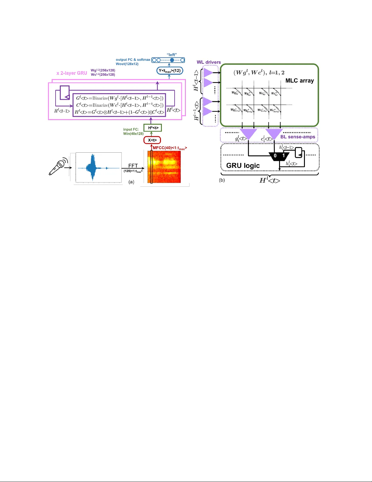
A binar y-activation, multi-level weight RNN and training algorithm for ADC-/D A C-free and noise-resilient processing-in-memory inference with eN VM Siming Ma Harvard University simingma@g.harvard.edu David Brooks Harvard University dbrooks@eecs.har var d.e du Gu- Y eon W ei Harvard University gywei@g.harvard.edu ABSTRA CT W e propose a new algorithm for training neural networks with binary activations and multi-level weights, which enables ecient processing-in-memory circuits with embedded nonvolatile mem- ories (eNVM). Binary activations obviate costly D ACs and ADCs. Multi-level weights le verage multi-level eN VM cells. Compared to existing algorithms, our method not only w orks for fee d-forward networks (e.g., fully-connected and convolutional), but also achieves higher accuracy and noise resilience for recurrent netw orks. In par- ticular , w e present an RNN-based trigger-word detection PIM accel- erator , with detailed hardware noise models and circu it co-design techniques, and validate our algorithm’s high inference accuracy and robustness against a variety of real hardwar e non-idealities. 1 IN TRODUCTION Processing-in-memory (PIM) architectures for hardware neural network (NN) inference have gained incr easing traction as they solve the memory b ottleneck of traditional von Neumann archi- tectures [ 32 ]. While PIM architectures apply to dierent types of memories, including SRAM and eDRAM, it is especially advan- tageous to use emb edded non-volatile memories (eNVM), due to their higher storage density and multi-level-cell (MLC) capability [ 3 , 20 , 33 ]. Moreover , their non-v olatility and p ower eciency are especially well suited for inference tasks that require relatively xed NN parameters. PIM with eN VMs not only avoids high-energy , long- latency , o-chip DRAM accesses by densely storing all NN parame- ters on-chip, it also minimizes inecient on-chip data mov ement and intermediate data generation by embedding critical multipli- cation and accumulation (MA C) computations within the memory arrays. The resulting highly-ecient MA C computations within the memory arrays are, howev er , analog in nature, which raises some issues. First, analog computations are sensitive to noise fr om the memory devices and circuits. Luckily , inherent noise r esilience of NN models ought to ameliorate this concern. Se cond and more importantly , typical NNs use high-precision neuron activations that require D ACs and ADCs in order to feed inputs to and resolve MA C outputs from the memor y arrays, respectively . These circuit blocks introduce signicant ar ea, power , and latency overheads. For example, the die photo in [ 40 ] shows the area of 5-bit input D ACs consume more than one thir d of the area of the SRAM PIM array . This translates to even greater relative overhead for an eN VM- based PIM. Thorough design space exploration of a ReRAM PIM architecture in [ 32 ] sho ws the optimal conguration is to shar e one 8-bit ADC across all 128 columns of a 128x128 memristor array . Y et, this single ADC still occupies 48 times the area and consumes 6.7 times the energy of the entire memristor array . In fact, given this high cost of ADCs and DA Cs, many PIM designs resort to feeding and/or resolving activations one bit at a time in a sequential fashion, which then r esults in large latency penalties [ 32 , 34 ]. Either way , the high overhead introduced by ADCs and DA Cs defeats the original goal of attaining speed, power , and area eciency by using PIM, which has recently drawn wide attention across the device, circuit, and algorithm communities [ 15 , 35 , 38 ]. Thirdly , weights of conventional NNs usually require higher resolution (e.g., 8 bits) than are available in typical MLCs (e.g., 2 or 3 bits), which requires each weight to b e across multiple memory cells and further degrades area eciency . Reducing bit precision of b oth activations and weights can miti- gate D AC and ADC overhead and reduce the number of cells ne eded for each weight. Hence, some PIM designs implement binar y neural networks (BNN), with both binary weights and binar y activations, obviating D ACs and ADCs entir ely , and only needing one single- level cell (SLC) p er weight [ 16 ]. How ever , BNNs ar e not optimal for two reasons. First, the most popular BNN training algorithms use the straight-through estimator (STE) to get around BNN’s indier- entiability problem during backpropagation [ 4 , 11 , 28 ]. Howev er , as we will show in Sections 4.1 and 4.2, STE for binarizing activations is eective for training feedforward NNs, such as fully-connecte d (FC) and convolutional NNs (CNN), but works po orly for recurrent NNs (RNN). Second, binary weights in BNNs ar e too stringent to maintain high inference accuracy and do not take full advantage of the MLC capabilities of eNVMs. This paper proposes an ADC-/DA C-free PIM architecture using dense MLC eNVMs (Figure 1(c)), which addresses all of the afore- mentioned issues of prior PIM designs. The major contributions of this work are: • T o enable this optimal PIM architecture, w e present a new noisy neuron annealing (NNA) algorithm to train NNs with binary activations (BA) and multi-level weights (MLW) that take full advantage of dense MLCs. This algorithm achieves higher inference accuracy than using STE to train BA-MLW RNNs. • W e design an ADC-/DA C-free trigger word detection PIM ac- celerator with MLC eN VM, using a BA-MLW gated recurrent unit (GRU). Simulation r esults demonstrate superior infer- ence accuracy and noise resilience compared to alternative algorithms. • Using detailed hardware noise models and circuit co-design techniques, we validate our NNA training algorithm yields high inference accuracy and robustness against a variety of real hardware noise sour ces. Siming Ma, David Brooks, and Gu-Y eon W ei X i X i + 1 Y j = ∑ i X i ⋅ W i , j Y j + 1 = ∑ i X i ⋅ W i , j + 1 ˜ Y j = f ( Y j ) ˜ Y j + 1 = f ( Y j + 1 ) DAC DAC ADC ADC f ( ⋅ ) f ( ⋅ ) WL-DACs BL-ADCs each high resolution weight may use a combination of many cells X i X i + 1 ˜ Y j ˜ Y j + 1 1/0 1/0 BL sense-amps (comparators) each multi-level weight uses a pair of MLC WL-drivers (a) (c) W + i , j W − i , j W + i + 1, j W − i + 1, j W + i , j + 1 W − i , j + 1 W + i + 1, j + 1 W − i + 1, j + 1 Y j = ∑ i X i ⋅ W i , j Y j + 1 = ∑ i X i ⋅ W i , j + 1 W i , j + 1 W i , j W i + 1, j W i + 1, j + 1 X i X i + 1 ˜ Y j ˜ Y j + 1 1/0 1/0 BL sense-amps (comparators) each binary weight uses a SLC WL-drivers (b) -1/+1 -1/+1 -1/+1 -1/+1 Y j = ∑ i X i ⋅ W i , j Y j + 1 = ∑ i X i ⋅ W i , j + 1 Figure 1: (a) The conventional PIM architecture with DA Cs and ADCs for high-precision activations and a combination of many cells for each high-resolution weight. ( b) an ADC-/DA C-free PIM architecture implementing BNNs, using SLCs for binary weights, and (c) the optimal ADC-/DA C-free PIM architecture implementing our BA-MLW NNs, using a pair of MLCs for each MLW . • W e further demonstrate the generality of our NNA algorithm by also applying it to feedfor ward networks. 2 BA CKGROUND MLC eNVM for PIM. Before we introduce the PIM architecture, it is important to rst review the technologies available for its critical building block – the memory array . Although the memory array can be built with conventional SRAM cells, it is more advantageous to use eN VM, including traditional embe dded Flash (eFlash) [ 8 ], or emerging resistive RAM (ReRAM) [ 33 ] and phase change memory (PCM) [ 3 ], or more r e cently , the purely-CMOS MLC eN VM (CMOS- MLC) [ 20 ]. Compared with SRAM, which is inherently binary (sin- gle level cells, SLC), eNVM’s SLCs oer much higher area eciency . Moreover , eNVM is often analog in nature that enables MLC capa- bility for even higher storage density . Programming eN VM typically involves a continuous change in the conductivity of the memory devices, enabling them to store multiple levels of transister channel current in the cases of eFlash and CMOS-MLC, or multiple le vels of resistor conductivity in the cases of ReRAM and PCM. The pro- gramming speed of eN VM is much slower than SRAM, but NN parameters are typically written infrequently and held constant during inference, rendering programming spee d non-critical for inference-only applications. In fact, eNVM’s non-volatility oers energy savings and obviates reloading weights at power-up . PIM for NN inference. A conv entional PIM architecture for NN inference is shown in Figure 1a [ 32 ]. The weight matrix of a NN is directly mapped into the memory array and, because weights for NNs typically r e quire high r esolution (e.g., ≥ 8 bits), multiple low er- resolution memory cells are often combined to represent one weight. This PIM structure can perform a matrix-vector multiplication in one step. Each input activation (i.e., 𝑋 𝑖 , 𝑋 𝑖 + 1 , . . . ) is simultaneously fed into individual wordlines as an analog voltage signal via a wordline D AC (WL-D A C), which then b ecomes a current through each memory cell proportional to the product of the input voltage and memory-cell conductance. MAC results are accumulated along corresponding sets of parallel bitlines (BLs) and resolved by column ADCs before being sent to digital nonlinear activation function units. A pair of columns are used to supp ort both p ositive and negative weight values and each column pair corresponds to a single neuron. Again, as discussed in Section 1, while these D ACs and ADCs support high-resolution activation, they impose large area and power ov erheads. Quantization and BNN. Many dierent NN quantization al- gorithms have been proposed to reduce the bit widths of w eights and/or activations while maximizing accuracy [ 11 , 19 , 28 ], in order to reduce storage and computation. For PIM, aggressiv e quantiza- tion can further relieve AD/D A resolution requirements for activa- tions. In particular , BNNs with 1-bit activations and weights, can translate into much simpler PIM circuits, as sho wn in Figure 1b (compared to the conventional PIM architecture in Figure 1a). Since the activations are binar y , WL-DA Cs and BL- ADCs in Figure 1a can be replaced by digital WL-drivers and conventional sense-amp comparators, respectively , both of which are compact peripheral components in standard memories. However , PIM implementations of BNNs have two major drawbacks. First, as shown in Figure 1b, bi- nary weights use eNVM cells as 1-bit SLCs, not taking advantage of their MLC capability . Second, the most popular existing algorithm for training binary activations uses STE [ 4 , 11 ], which is eective for feedfor ward NNs, but performs poorly on RNNs. 3 TRAINING BA-MLW NNS FOR OPTIMAL PIM IMPLEMEN T A TION T o avoid D ACs and ADCs and fully le verage MLCs, we propose a BA -MLW NN structure, shown in Figure 1c, as an optimal design for PIM. For simplicity , memory devices are illustrated as resis- tor cells (omitting access transistors), corresponding to ReRAM or PCM, with multi-level weights encodes via their conductance val- ues; other eNMV technologies, such as eFLASH and CMOS-MLC, directly encode weights into access transistor channel currents. The current dierence acr oss a pair of cells represent one postive or negative weight value. Moreover , binary activation (BA) only requires digital WL-drivers and sense-amps, obviating expensive D ACs and ADCs. In order to ee ctively train BA-MLW NNs, we propose a new algorithm that achieves high accuracy and resilience to quantization and noise for both fe edfor ward and recurrent NNs. A binary-activation, multi-level weight RNN and training algorithm for ADC-/DA C-free and noise-resilient processing-in-memory inference with eNVM 3.1 Training binary activations (BA) Binarizing the activations while maintaining high performance is challenging, be cause it not only restricts the expressive capacity of the neurons, but also introduces discrete computation no des that preclude gradient pr opagation during training. W e rst review the STE algorithm prior to introducing our proposed BA training algorithm. Reviewing STE. STE applies to a stochastic binary neur on (SBN) [ 4 ]. During forward pr opagation of training, each neuron generates a binary output from a Bernoulli sample 𝑥 SBN = ( 1 , with probability 𝑝 = sigmoid ( 𝑠 · 𝑥 ) 0 , with probability 1 − 𝑝 (1) in which 𝑥 is a pre-activation from the linear MAC and the logistic sigmoid function has a tunable slope 𝑠 [ 7 ]. The SBN function is discrete with random sampling and, thus, does not have a well- dened gradient. Hence, STE simply passes through the gradient of the continuous sigmoid function during backpropagation 𝜕𝐿 𝜕𝑥 = 𝜕𝐿 𝜕𝑥 SBN · sigmoid ′ ( 𝑠 · 𝑥 ) (2) in which 𝐿 is the loss function. In other words, it ignores the random discrete sampling process, and pretends the for ward propagation im- plements a sigmoid function. The issue with STE is that propagating gradients w .r .t. the sample-independent mean ( 𝑥 SBN = sigmoid ( 𝑠 · 𝑥 ) ) while ignoring the random sampling outcome can cause discrepan- cies b etween the forward and backward passes [ 12 ]. In fact, STE is a biased estimator of the expe cted gradient, which cannot even guar- antee the correct sign when back-pr opagating through multiple hidden layers [ 4 ]. Nonetheless, STE has been found to work better in practice than other more complicate d gradient estimators for feedfor ward NNs [ 4 ], which we also verify in Section 4.2. Howev er , as shown in Section 4.1, STE performs poorly when training RNNs with BAs. Proposed noisy neuron annealing (NNA) algorithm. W e use the following noisy continuous neuron (NCN) function during the forward pass of training 𝑥 NCN = sigmoid ( 𝑥 + 𝑛 train 𝜏 ) (3) in which we add an i.i.d. zero-mean Gaussian random variable (RV) 𝑛 train ∼ 𝑁 ( 0 , 𝜎 2 train ) to each pre-activation before passing into a continuous sigmoid function with temperature 𝜏 . Equation 3 can b e broken down into two steps: (i) a noise inje ction step, ˜ 𝑥 = 𝑥 + 𝑛 train , and (ii) a continuous r elaxing step, 𝑥 NCN = sigmoid ( ˜ 𝑥 / 𝜏 ) . This noise injection step – random noise added into pre-activations – corresponds to quantization noise, due to binarizing activations and quantizing weights, that ows for ward through the MA C. Therefore, if we train the NN with noise explicitly added into pre-activations, the NN would develop r esilience to these quantization errors. The continuous relaxing step is inspired by the Gumbel-softmax trick [ 12 , 21 ], which uses a sharpened sigmoid to appro ximate the binar y step function while still allowing smooth gradients to ow . As Section 4.1 will show , it is important to start fr om a large value of the hyperparameter 𝜎 train to begin training with large noise and then anneal down to a smaller value, hence , the name of our training strategy – “noisy neuron annealing” (NNA) algorithm. Related to the additive noise in variational auto encoders, the Gaussian noise distribution complies to the “mean and variance” form required by the re-parameterization trick [ 21 ]. This has a nice Gaussian gradient identity property [ 30 ] that allows reversing the order between taking the expectation and taking the derivative . Combined with the continuous relaxation step, backpropagation through the entire NCN function does not encounter any discrete or sampling nodes: 𝜕𝐿 𝜕𝑥 = 𝜕𝐿 𝜕𝑥 NCN · sigmoid ′ ( 𝑥 + 𝑛 train 𝜏 ) (4) During inference, we use the following noisy binar y neuron (NBN) function: 𝑥 NBN = ( 1 , if 𝑥 + 𝑛 eval > 0 0 , otherwise (5) which also has an additive i.i.d. Gaussian RV 𝑛 eval ∼ 𝑁 ( 0 , 𝜎 2 eval ) , but replaces the continuous sigmoid in NCN with a discrete step func- tion. In Sections 4.1 and 4.2, we evaluate the noise resilience of trained NNs by sweeping 𝜎 eval . Prior work has studied the regularization eect of noise injection regarding its impact on NN generalization and noise resilience [ 1 , 13 , 25 , 29 ]. They use T aylor expansion of the loss function to show that adding Gaussian noise is akin to adding an extra regularization penalty term to the original loss function 𝐿 , such that the eective loss becomes ˜ 𝐿 = 𝐿 + 𝑃 = 𝐿 + 1 2 𝜎 2 train  𝑖 ( 𝜕𝐿 𝜕𝑥 𝑖 ) 2 (6) where 𝑥 𝑖 refers to a certain noise-injected node. In our case, 𝑥 𝑖 in- cludes all pre-activations. The regularization term, 𝑃 , penalizes large gradients of 𝐿 w .r .t. noise-injected nodes, encouraging these nodes to nd “atter regions” of the solution space that are less sensitive to noise perturbations. Hyp erparameter 𝜎 train controls the tradeo between reducing the raw error 𝐿 and enhancing noise resilience. Specically , for NCN activations to counteract the noise, they tend to give up the highly-expressiv e but noise-prone transition region of the sigmoid and, instead, dev elop a bimodal pre-activation dis- tribution to push them into the saturated regions, close to 1 or 0, that are highly immune to noise [ 31 ]. Equation 6 also provides a quantitative metric to estimate the noise resilience a NN acquir es during training. W e derive a detailed form to calculate this penalty term in Section 4.1 to compare amongst dierent NNs. T able 1: An example mapping 7-le vel weights into the 𝐼 + cell and 𝐼 − cell current magnitudes of a pair of 4-level cells. 𝐼 fs is the full-scale current that corresponds to 𝛼 . weight − 𝛼 − 2 3 𝛼 − 1 3 𝛼 0 1 3 𝛼 2 3 𝛼 𝛼 𝐼 − cell 𝐼 fs 2 3 𝐼 fs 1 3 𝐼 fs 0 0 0 0 𝐼 + cell 0 0 0 0 1 3 𝐼 fs 2 3 𝐼 fs 𝐼 fs Siming Ma, David Brooks, and Gu-Y eon W ei Figure 2: (a) BA -MLW GRU architecture with an input FC and 2 GRU layers and (b) the PIM implementation of a GRU layer . 3.2 Training multi-level weights (MLW) Our NNA algorithm not only endows the NN with high resilience to binarizing activations, but also enables MLW s to leverage dense MLCs with high inference accuracy . Each weight can be quantized down to a small number of levels capable of encoding with one pair of MLCs (Figure 1c), as opposed to ne eding to combine multiple memory cells for high-resolution weights (Figure 1a). T o quantize MLW s from full-precision (FP) weights, we rst determine a suitable clipping range [ − 𝛼 , 𝛼 ] for each weight matrix based on the weight distribution statistics from pre-training with FP weights. Then during ne-tuning with weight quantizations, w e clip each weight matrix into [ − 𝛼 , 𝛼 ] prior to quantizing the weights into evenly-spaced levels within this range. W e follow the same practice as [ 11 ] for training, i.e., we use the quantized w eights in the forward pass, but still keep the FP weights and accumulate gradients onto FP weights in the backward pass. After training is complete, the FP weights can be discarded and only the quantized weights are used for inference. For the special cases of 3- and 2-level weights, we use the training algorithm in [ 19 ] for 3-level (ternary) and [28] for 2-level (binary) weights. T able 1 shows how to represent a 7-level w eight via the current dierential across a pair of 4-level (2-bit) MLCs. Following the same principle, a 15-level w eight can b e encoded with a pair of 8-level (3-bit) MLCs, while a 3-level weight can use a pair of binary cells (1-bit, SLC). 4 APPLICA TION CASE ST UDIES W e present two case studies that apply our NNA algorithm to (1) an RNN for a trigger word detection task and (2) a feedforward NN for handwritten digit recognition. W e focus on the rst case study to thoroughly demonstrate the merits of a BA -MLW RNN trained using the NNA algorithm. The second case study conrms the algorithm further generalizes to feedfor ward NNs. 4.1 A trigger wor d detection PIM accelerator using BA-MLW GRU with MLC eN VM Trigger wor d detection is an important always-ON task for spe ech- activated edge devices, for which power and cost eciency is para- mount. W e use the Sp eech Commands dataset from [ 36 ], which consists of ov er 105,000 audio clips of various wor ds uttered by thousands of dierent people, with a total of 12 classication cate- gories: 10 designated keywords, silence, and unkno wn words. W e rst present the architectural designs of the NN and PIM accelerator (Section 4.1.1), then elaborate on the software training results using dierent training methods (Section 4.1.2), and nally e valuate ex- pected hardware performance with detaile d noise models (Section 4.1.3). 4.1.1 The architecture of the NN and PIM accelerator. The NN model structure. RNNs are well-suited to this spe ech-recognition task. Figure 2a illustrates a 2-layer gated recurrent unit ( GRU) [ 6 ] with BA and MLW . W e rst perform FFT (window=16ms, stride=8ms) on the raw audio signals and then extract 40 Mel-frequency cepstral coecients (MFCC) per 8ms timestep. Each MFCC vector passes through an input FC layer that encodes it into a 128 dimensional binary vector as the input to the rst layer of a 2-lay er stacked GRU (both layers use 128 dimensional vectors). W e use the following modied version of GRU equations [26]: e 𝐺 𝑙 < 𝑡 > = 𝑊 𝑔 𝑙 · [ 𝐻 𝑙 < 𝑡 − 1 > , 𝐻 𝑙 − 1 < 𝑡 > ] (7) 𝐺 𝑙 < 𝑡 > = 𝑓 ( e 𝐺 𝑙 < 𝑡 > ) (8) e 𝐶 𝑙 < 𝑡 > = 𝑊 𝑐 𝑙 · [ 𝐻 𝑙 < 𝑡 − 1 > , 𝐻 𝑙 − 1 < 𝑡 > ] (9) 𝐶 𝑙 < 𝑡 > = 𝑓 ( e 𝐶 𝑙 < 𝑡 > ) (10) 𝐻 𝑙 < 𝑡 > = 𝐺 𝑙 < 𝑡 > ⊗ 𝐻 𝑙 < 𝑡 − 1 > + ( 1 − 𝐺 𝑙 < 𝑡 > ) ⊗ 𝐶 𝑙 < 𝑡 > (11) where 𝑡 denotes the timestep, 𝑙 is the layer number , and the gate 𝐺 𝑙 < 𝑡 > ( 𝑙 = 1 , 2 ), candidate 𝐶 𝑙 < 𝑡 > ( 𝑙 = 1 , 2 ), hidden state 𝐻 𝑙 < 𝑡 > ( 𝑙 = 1 , 2 ), A binary-activation, multi-level weight RNN and training algorithm for ADC-/DA C-free and noise-resilient processing-in-memory inference with eNVM and the input encoding 𝐻 0 < 𝑡 > are all 128 dimensional activation vectors, trained using our NNA algorithm. The activation function 𝑓 refers to NCN (Equation 3) during training, and NBN (Equation 5) for evaluation, and simply uses the binar y step function for PIM deployment (Figure 2a and 2b). Compared with the original GRU equations from [ 6 ], we remove the reset gate since it has minimal eect on the accuracy of this task, but greatly simplifes circuit design (Figure 2b). After the GRU processes inputs from all timesteps, the nal timestep output of the top layer feeds into an output FC layer followed by a 12-way softmax that yields the classication. PIM circuit design for the GRU. The BA-MLW GRU equations can be mapped into compact PIM circuits shown in Figure 2b . The MLC array implements MA C computations and the column sense- amps resolve the binarized 𝐺 𝑙 < 𝑡 > and 𝐶 𝑙 < 𝑡 > . 𝐺 𝑙 < 𝑡 > serves as the multiplexer selection signal (since 1 − 𝐺 𝑙 < 𝑡 > = ! 𝐺 𝑙 < 𝑡 > in Equation 11 for binary signals) to cho ose either to keep the binary hidden state saved from the pre vious timestep or to update it with the current binary candidate state. Since all analog MA C signals are encapsu- lated inside the MLC array , all input/output interface signals are binary , and the GRU logic outside the array is totally digital, this PIM design do es not require any ADCs or DA Cs . Noise-induced loss penalty terms for GRU. For the GRU , we can deriv e the noise-induced regularization penalty term 𝑃 in Equa- tion 6 by taking the derivatives of loss 𝐿 w .r .t. the pre-activations of candidates ( e 𝐶 𝑙 < 𝑡 > ) and gates ( e 𝐺 𝑙 < 𝑡 > ). 𝑃 = 1 2 𝜎 2 𝑡 𝑟 𝑎𝑖𝑛  𝑖 ,𝑡 ,𝑙 ( 𝜕𝐿 𝜕ℎ 𝑙 𝑖 < 𝑡 > ) 2 · { 𝑃 𝑔 + 𝑃 𝑐 } (12) 𝑃 𝑔 = [ ( ℎ 𝑙 𝑖 < 𝑡 − 1 > − 𝑐 𝑙 𝑖 < 𝑡 > ) · sigmoid ′ ( e 𝑔 𝑙 𝑖 < 𝑡 > ) ] 2 (13) 𝑃 𝑐 = [ ( 1 − 𝑔 𝑙 𝑖 < 𝑡 > ) · sigmoid ′ ( e 𝑐 𝑙 𝑖 < 𝑡 > ) ] 2 (14) where a lower case letter with subscript 𝑖 = 0 ∼ 127 denotes one ele- ment of the corresponding uppercase vector , and 𝑃 𝑔 and 𝑃 𝑐 regu- larize gates and candidates, respectively . The forms of Equations 13 and 14 have intuitive interpr etations when minimizing them during training. T o minimize 𝑃 𝑔 , one way is to reduce the derivative of the gate ( sigmoid ′ ( e 𝑔 𝑙 𝑖 < 𝑡 > ) ) by pushing e 𝑔 𝑙 𝑖 < 𝑡 > away from zero (the steep slope region of sigmoid), so that the gate is rmly ON or rmly OFF; alternatively , it can try to make the candidate of the current timestep 𝑐 𝑙 𝑖 < 𝑡 > equal to the hidden state of the previous timestep ℎ 𝑙 𝑖 < 𝑡 − 1 > , such that the new hidden state ℎ 𝑙 𝑖 < 𝑡 > would be the same regardless of e 𝑔 𝑙 𝑖 < 𝑡 > . Either way , minimizing 𝑃 𝑔 makes ℎ 𝑙 𝑖 < 𝑡 > immune to noise injected into e 𝑔 𝑙 𝑖 < 𝑡 > . T o minimize 𝑃 𝑐 , train- ing will either reduce the gradient of candidate ( sigmoid ′ ( e 𝑐 𝑙 𝑖 < 𝑡 > ) ), by pushing e 𝑐 𝑙 𝑖 < 𝑡 > into the saturated at regions of sigmoid, or try to turn on the gate 𝑔 𝑙 𝑖 < 𝑡 > to preser ve the hidden state from the previous timestep ℎ 𝑙 𝑖 < 𝑡 − 1 > disregarding the new candidate 𝑐 𝑙 𝑖 < 𝑡 > . Either way , it desensitizes ℎ 𝑙 𝑖 < 𝑡 > to noise injected into e 𝑐 𝑙 𝑖 < 𝑡 > . Equa- tions 12–14 provide a quantitative metric to assess the resilience to quantization and noise in a traine d GRU, which we use to compare dierent training schemes. 4.1.2 Soware training results. T o quantitatively compare NN accu- racy and noise-resilience trained with dierent methods, we inject T able 2: Loss penalty terms of the 4 NNs in Figure 3a. Network FP baseline NNA( 𝜎 𝐿 ) NNA( 𝜎 𝐿 → 𝜎 𝑆 ) NNA( 𝜎 𝑆 ) Pg+Pc 1.0000 0.5034 0.5018 0.8272 the same type of Gaussian training noise during inference and sweep the noise sigma – a common practice adopted in previous NN noise-resilience studies [ 5 , 10 , 17 , 24 , 39 ]. W e rst compare dierent methods of binarizing activations, then explore dier ent quantization levels for the weights, and, nally , compare RNN train- ing performance using our NNA algorithm versus the popular STE algorithm. Results are summarized in Figure 3. Comparing training schemes for binarizing activations. As a full-precision (FP) baseline, w e rst train the NN with FP sig- moid activations and FP weights, without noise injection or quan- tization. During inference, we add noise 𝑛 eval ∼ 𝑁 ( 0 , 𝜎 2 eval ) to its pre-activations and evaluate it with b oth FP sigmoid activations (baseline- 𝐴 FP - 𝑊 FP , black), and binarized activations (baseline- 𝐵𝐴 - 𝑊 FP , yellow ), shown in Figure 3a. Trained without noise injection, baseline- 𝐴 FP - 𝑊 FP cannot maintain its high accuracy at large 𝜎 eval , making it vulnerable to quantization errors, leading to the po or performance of baseline- 𝐵𝐴 - 𝑊 FP . T o endow the NN with resilience to quantization errors, we use our NNA algorithm and retrain from the FP sigmoid baseline (which is a good initialization point to sp eed up retraining). Initially , we use large training noise 𝜎 train = 𝜎 𝐿 = 1 . 6 , and plot the inference accuracy with BAs and 7-lev el weights (NNA( 𝜎 𝐿 )- 𝐵𝐴 - 𝑊 7 , purple) in Figure 3a. Results show high accuracy across a wider range of 𝜎 eval than baseline- 𝐵𝐴 - 𝑊 FP , demonstrating stronger resilience to quantization errors. How ever , the accuracy peaks at a large 𝜎 eval around 𝜎 𝐿 , and lower at small 𝜎 eval , because it is traine d to minimize its loss in the presence of this large additiv e noise. This noise-resilience prole might suit certain noisy cir cuit environments, e.g., noisy power supply . In order to also achieve high accuracy at small 𝜎 eval , we anneal 𝜎 train down to a small 𝜎 train = 𝜎 𝑆 and further retrain. As shown in Figure 3a (NNA( 𝜎 𝐿 → 𝜎 𝑆 )- 𝐵𝐴 - 𝑊 7 , red), peak accuracy is achieved at smaller 𝜎 eval , demonstrating the ecacy of NNA with annealing (from 𝜎 𝐿 to 𝜎 𝑆 ). In comparison, directly retraining with 𝜎 𝑆 from the baseline (NNA( 𝜎 𝑆 )- 𝐵𝐴 - 𝑊 7 , green), without the intermediate 𝜎 𝐿 stage, results in much worse accuracy and noise tolerance than NNA with annealing. In practice, we nd the choices of the hyperparameter 𝜎 train quite exible. For the initial large noise, we use a 𝜎 𝐿 to be about 20% of the standard deviation (STD) of the inher ent pre-activation distribution, corresponding to 𝜎 𝐿 = 1 . 6 for this GRU, though a wide range of values all work similarly well; for the annealed noise, we nd 𝜎 𝑆 = 0 ∼ 0 . 5 all achieves optimal results. For temp erature 𝜏 in NCN, we nd 0 . 3 to b e optimal: If too small, RNN’s gradient explodes. If too large, BA is not suciently approximated. Loss penalty term interpretations. T o understand why the an- nealing procedure of NNA is critical, we compare the loss penalty terms ( 𝑃 𝑔 + 𝑃 𝑐 from Equation 13 and 14) of the four networks in Figure 3a. Sho wn in T able 2, we normalize them by the penalty value of baseline- 𝐴 FP - 𝑊 FP , since only the relative values matter for comparison. After retraining with 𝜎 𝐿 , NNA( 𝜎 𝐿 )- 𝐵𝐴 - 𝑊 7 ’s penalty Siming Ma, David Brooks, and Gu-Y eon W ei 0 . 0 0 . 5 1 . 0 1 . 5 2 . 0 2 . 5 3 . 0 3 . 5 sigma of additive G aussian noise during inference 20 40 60 80 inference accuracy ( training stage trajecto ries-OursRed baseline- A FP - W FP baseline- BA - W FP NNA(  S )- BA - W FP NNA(  L )- BA - W 7 NNA(  L !  S )- BA - W 7 0 . 0 0 . 5 1 . 0 1 . 5 2 . 0 2 . 5 3 . 0 3 . 5 sigma of additive G aussian noise during inference 20 40 60 80 inference accuracy ( Our algo rithm with di ↵ erent w eight quantization levels-OursRed NNA(  L !  S )- BA - W FP NNA(  L !  S )- BA - W 7 NNA(  L !  S )- BA - W 5 NNA(  L !  S )- BA - W 3 NNA(  L !  S )- BA - W 2 0 . 0 0 . 5 1 . 0 1 . 5 2 . 0 2 . 5 3 . 0 3 . 5 sigma of additive G aussian noise during inference 20 40 60 80 inference accuracy ( Our metho d vs straight-through-estimato r algo rithm-OursRed NNA(  L !  S )- BA - W 7 STE( s =1 )- BA - W FP STE( s =3 )- BA - W FP STE( s =1 ! 3 )- BA - W FP Inference accuracy (%) σ e va l Evaluation noise σ e va l Evaluation noise σ e va l Evaluation noise (a) (b) (c) 0 0.25 0.5 0.75 1. 0 86 88 90 92 94 Zoom 0 . 0 0 . 5 1 . 0 1 . 5 2 . 0 2 . 5 3 . 0 3 . 5 sigma of additive G aussian noise during inference 20 40 60 80 inference accuracy ( training stage trajecto ries-OursRed baseline- A FP - W FP baseline- BA - W FP NNA(  S )- BA - W FP NNA(  L )- BA - W 7 NNA(  L !  S )- BA - W 7 0 . 0 0 . 5 1 . 0 1 . 5 2 . 0 2 . 5 3 . 0 3 . 5 sigma of additive G aussian noise during inference 20 40 60 80 inference accuracy ( Our algo rithm with di ↵ erent w eight quantization levels-OursRed NNA(  L !  S )- BA - W FP NNA(  L !  S )- BA - W 7 NNA(  L !  S )- BA - W 5 NNA(  L !  S )- BA - W 3 NNA(  L !  S )- BA - W 2 94 92 90 88 86 0.25 0.5 0.75 1.0 0 0 . 0 0 . 5 1 . 0 1 . 5 2 . 0 2 . 5 3 . 0 3 . 5 sigma of additive G aussian noise during inference 20 40 60 80 inference accuracy ( Our metho d vs straight-through-estimato r algo rithm-OursRed NNA(  L !  S )- BA - W 7 STE( s =1 )- BA - W FP STE( s =3 )- BA - W FP STE( s =1 ! 3 )- BA - W FP Figure 3: Inference accuracy vs 𝜎 𝑒 𝑣𝑎𝑙 of evaluation noise of GRUs trained with dierent metho ds (plotting the mean accuracy surrounded with the ranges of mean ± STD and max/min). (a) compares 4 networks trained through dierent stages, in which the baseline network is evaluated with both FP activations and BAs, (b) compares dierent weight quantization levels, using NNA algorithm, and (c) compares NNA with STE algorithm. Except for baseline- 𝐴 𝐹 𝑃 - 𝑊 𝐹 𝑃 that uses FP activations, all the other curves are evaluated with BAs using NBN Equation 5. term reduces to half of the baseline penalty , e xplaining its higher resilience to noise and quantization errors. After further retrain- ing with annealed 𝜎 𝑆 , NNA( 𝜎 𝐿 → 𝜎 𝑆 )- 𝐵𝐴 - 𝑊 7 maintains this small penalty value, even though 𝜎 𝑆 provides less regularization eect – the smaller multiplier 𝜎 2 𝑆 in Equation 12 ( compared to previous 𝜎 2 𝐿 ) makes the retraining prioritize reducing the raw error (thus higher peak accuracy) over enhancing noise resilience. This means the network can still “memorize ” its previous large-noise training regularization eect even after annealing to ne-tune with smaller noise. In contrast, without the intermediate “e xp erience” of large noise training, NNA( 𝜎 𝑆 )- 𝐵𝐴 - 𝑊 7 has much less regularization eect to reduce its loss penalty . It should also be pointed out that if e valuate d with FP activations and zero noise, all these networks achie ve similarly high accuracy as the purely FP sigmoid network, but their accuracy and noise resilience are dramatically dier ent after using binar y activations. This implies that trained through dierent stages, the 4 networks in Figure 3a nd distinct regions in the global solution space: re- training with 𝜎 𝐿 nds a promising solution region that’s insensitive to quantization errors, while the further ne-tuning with 𝜎 𝑆 only does a lo cal search to optimize accuracy at the small noise range; in contrast, training without noise injection or only with small noise will not discover the solution region that’s resilient to noise and quantization due to lack of regularization penalty . W eight quantization levels. Figure 3b shows the GRU’s per- formance across dierent numbers of weight quantization levels and conrms the high resilience to weight quantization oered by our NNA algorithm. The r esulting performance of 7-level (imple- mented with a pair of 4-level cells) and 5-level (a pair of 3-level cells) quantization are almost the same as using FP weights. GRUs with 7-le vel weights achieve the highest peak accuracy at the lower end of 𝜎 eval range. Accuracy for GRUs with ternary weights (a pair of 2-level cells) degrades more quickly as 𝜎 eval increases. In contrast, GRUs with binary weights, which can be implemented with SRAMs), suer the most accuracy degradation across the en- tire 𝜎 eval range. Our NNA algorithm’s high resilience to weight quantization makes it possible to use a pair of 3 or 4-level MLCs to achieve performance comparable to GRUs with FP w eights. Even GRUs with tenar y weights can achieve relatively high inference accuracy for applications with small 𝜎 eval . Therefore, our optimal PIM architecture (Figur e 1c) avoids combining multiple cells to achieve high-resolution weights (Figure 1a, [ 32 ]), thereby saving area and simplifying circuit design. NNA vs STE. W e also experiment with SBN trained with STE, and compare its p erformance with our NNA algorithm in Figure 3c. W e tr y 3 dierent settings for slope 𝑠 : 𝑠 = 1 (yello w), 𝑠 = 3 (blue), and annealing 𝑠 from 1 to 3 ( 𝑠 = 1 → 3 , green) [7]. Even with FP weights, all three GRUs trained with STE achieve worse inference accuracy compared to using NNA (NNA( 𝜎 𝐿 → 𝜎 𝑆 )- 𝐵𝐴 - 𝑊 7 , red). W e should also p oint out an important distinction between the forms of SBN (Equation 1) and our NCN (Equation 3): SBN only has one parameter 𝑠 , whereas NCN has two degrees of freedom using 𝜏 and 𝜎 𝑡 𝑟 𝑎𝑖𝑛 . On one hand, SBN uses 𝑠 to control the sigmoid slope (corresponding to 1 / 𝜏 in NCN), and similar to 𝜏 , we nd 𝑠 needs to be no greater than about 3, in or der not to run into exploding gradient problem. On the other hand, 𝑠 also contr ols the stochasticity of the Bernoulli sampling: a smaller 𝑠 introduces more randomness thus a higher noise resilience range, as can be se en from Figure 3c, comparing 𝑠 = 1 , 𝑠 = 3 and 𝑠 = 1 → 3 . Howev er , SBN cannot seperately control the the sigmoid slope and the sto chasticity . In contrast, our NCN has independent controls: 𝜏 is chosen to approximate binary outputs while avoiding exploding gradients, whereas the magnitude of noise injection is seperately controlled by 𝜎 𝑡 𝑟 𝑎𝑖𝑛 . This exiblity enables us to eectively implement NNA algorithm’s annealing procedure using NCN. From a mathematical rigor p oint of view , in contrast to the Gauss- ian RV s use d in NCN, the Bernoulli RV s used in SBN do not comply with the “location-scale ” distribution required for using the repa- rameterization trick [ 21 ]. Therefore, it is mathematically illegal for STE to change the order between taking expectation and taking derivative for Bernoulli RV s (Equation 2). Increasing the slope 𝑠 can alleviate the discrepancy between the forward and backward pass of SBN (making the math less wrong, which explains the higher accuracy with 𝑠 = 3 in Figure 3c), but due to the lack of separate con- trols, changing 𝑠 inevitably changes both the sampling randomness A binary-activation, multi-level weight RNN and training algorithm for ADC-/DA C-free and noise-resilient processing-in-memory inference with eNVM and sigmoid’s gradient, and 𝑠 cannot be too large which will cause exploding gradients. 4.1.3 Hardware noise model and validation results . Need for accurate hardware noise models. So far we have used the same type of additive random Gaussian noise for both training and inference as 𝑁 train and 𝑁 eval in Figure 3, consistent with prior work that evaluate and compar e NN noise resilience [ 5 , 10 , 17 , 24 , 39 ]. While prior hardware noise mo deling work generally over- simplify by lumping all the noise sources into a single random Gaussian RV , real circuits have a variety of noise sources with properties dierent from these additiv e Gaussian RV s, mandating realistic mo dels to faithfully evaluate their impact on hardware inference accuracy . T o evaluate how real cir cuit noise impacts inference accuracy , we account for the detailed proles of three important sources of physical noise in PIM circuits shown in Figure 4: (1) the weight noise 𝑁 MLC due to variability of eNVM devices, (2) an oset error 𝑁 OS due to de vice mismatch in the sensing circuitr y , and (3) a white noise source 𝑁 white from thermal and shot noise of the circuits. In the follo wing subsections, we rst elaborate on the distinctive char- acteristics of these three noise sources and present our simulation methodology of the overall noise model; then we introduce the devices and circuit designs of the PIM implementation used for deriving the statistics to build the noise model; nally , we present the hardware validation experiment results. Figure 4: Illustration of detailed circuit-lev el noise sour ces in PIM hardware. (1) 𝑁 MLC comes from eN VM device manufacturing and program- ming variability , modeled as noise in programmed MLC weight levels, i.e., p er-cell static weight error 𝛿𝑊 + 𝑘 ,𝑖 or 𝛿𝑊 − 𝑘 ,𝑖 deviating from the intended/ideal value 𝑊 + 𝑘 ,𝑖 or 𝑊 − 𝑘 ,𝑖 (Figure 4). Depend- ing on input activations of each timestep, each cell’s weight error selectively contributes noise to the total w eight noise of 𝑁 MLC = Σ 𝑘 ( 𝛿𝑊 + 𝑘 ,𝑖 − 𝛿𝑊 − 𝑘 ,𝑖 ) · 𝑋 𝑡 𝑘 added to each corr esponding element of MA C pre-activations. (2) 𝑁 OS models transistor-mismatch-induced oset as a sense- amp input-referred static error . Each sense-amp ’s random oset is determined after fabrication, which adds a xed asymmetric bias term into the MA C computation associated with the comparisons of each sense-amp. This oset prov es to be detrimental to inference accuracy due to its lack of dynamic randomness, but most prior noise-modeling studies overlook this important source of error . Among the few papers that address this oset error , [ 24 ] simpli- es it into a Gaussian RV , lumped with other noise sources by adding their variances together , and proposes p er-chip, post-fabrication retraining; [ 2 ] uses on-chip digital calibration circuitry to cancel the oset after fabrication. In contrast, we de dicate the realistic static noise model 𝑁 OS to each oset error , and le verage a simple yet eective circuit technique that avoids the need for individ- ual retraining or the overhead of oset calibration. Our solution is to randomly ip the polarity of the added 𝑁 OS using a set of switches controlled by a pseudo random number generator (PRNG), as shown in Figure 4, such that each xed 𝑁 OS magnitude is pre- sented to each element of pre-activations with a random polarity per sense-amp comparison p er timestep, thereby converting the eect of each sense-amp oset into a Bernoulli RV . Compared with the smooth “bell-shape d” Gaussian noise with which our NNs are trained, Bernoulli distributions have very dierent forms, but they can guarantee p er-element zero-mean and dynamic randomness across timesteps. These are the traits of noise that NNs trained with our NNA algorithm are surprisingly r esilient to, as we will show in our validation experiments. (3) 𝑁 white represents thermal and shot noise from the cir cuits, which are dynamic random white noise, modeled as an input- referred Gaussian noise source at each sense-amp. This is the only truly random and dynamic source of hardware noise, with exactly the same properties as the Gaussian noise used for training. The overall noise mo del accounts for the three aforementioned noise sources, such that the total noise added into each element of pre-activations at each timestep is: 𝑁 MLC ± 𝑁 OS + 𝑁 white = Σ 𝑘 ( 𝛿𝑊 + 𝑘 ,𝑖 − 𝛿𝑊 − 𝑘 ,𝑖 ) · 𝑋 𝑡 𝑘 + ( − 1 ) polarity · 𝑁 OS + 𝑁 white . When simulating the inference performance of a single chip, 𝑁 OS , 𝛿𝑊 + 𝑘 ,𝑖 and 𝛿𝑊 − 𝑘 ,𝑖 are determined/static after fabrication and weight pr ogramming, so we only randomly sample them once and x them during inference on all validation examples; 𝑁 white is dynamic and so we randomly generate a new sample for each sense-amp comparison; the PRNG dynamically generates a random selection of 𝑝𝑜 𝑙 𝑎𝑟 𝑖 𝑡 𝑦 to add or subtract the xed 𝑁 OS magnitude for each corresponding sense-amp compari- son. W e validate hardware performance at the presence of all these noise sources by simulating cycle-accurate inference across GRU timesteps. Device mo dels and circuit simulations. For eNVM de vices, we evaluate three promising emerging eNVMs (ReRAM, PCM, and CMOS-MLC) and model their corresponding 𝑁 MLC based on mea- sured data from [ 33 ], [ 3 ], and [ 20 ], respectively . W e design and simulate all peripheral cir cuits targeting a 16nm FinFET technology [ 37 ]. The sensing circuits that resolve BAs adopt the dynamic bitline discharge technique commonly used in memory reading circuitry , Siming Ma, David Brooks, and Gu-Y eon W ei T able 3: Summary of hardware noise validation results. Impact of 𝑁 OS (w/o 𝑁 MLC ) 𝑁 white -only (baseline) 𝑁 white + 𝑁 OS xed polarities 𝑁 white + 𝑁 OS ipping polarities Accuracy range (%) 91 . 76 ± 0 . 23 91 . 26 ± 0 . 22 91 . 86 ± 0 . 24 Impact of eNVM (w/ all noise sources) PCM ReRAM CMOS-MLC Accuracy range (%) 91 . 60 ± 0 . 34 91 . 71 ± 0 . 27 91 . 60 ± 0 . 29 with the self-timed StrongArm-type sense-amp from [ 23 ]. Sensing via variable bitline discharge time automatically handles the wide statistical range of bitline currents resulting from PIM-based MA C computations. Transistor sizes in the sense-amp pose a tradeo between ar ea versus 𝑁 OS , i.e., enlarging the transistor sizes can reduce 𝑁 OS at the expense of a larger sense-amp area overhead. W e use Monte Carlo simulations to measure the 𝑁 OS of a range of sense-amp sizes, and evaluate their impacts on infer ence accuracy . Figure 5: Hardwar e inference accuracy distributions of the trigger word detection PIM accelerator using three promis- ing eNVM technologies, validated with the detailed noise models in Figure 4. V alidation results are summarized in T able 3 and Figure 5. W e choose NNA( 𝜎 𝐿 → 𝜎 𝑆 )- 𝐵𝐴 - 𝑊 7 as the optimal design target for circuit implementation and evaluation of the NNA algorithm’s resilience to hardware noise . W e establish a baseline accuracy ( 𝑚𝑒 𝑎𝑛 ± STD = ( 91 . 76 ± 0 . 23 ) %) corresponding to when only 𝑁 white is present and both 𝑁 OS and 𝑁 MLC are zero . This baseline accuracy is on par with the peak software inference accuracy in Figure 3. The magnitude of 𝑁 white for r eal circuits turns out to be too small to have measurable impacts on accuracy . W e rst fo cus on exploring the performance impact of 𝑁 OS and the polarity ipping circuit technique. W e then simulate with the entir e noise model across three promising eN VM technologies. As summarized by the upper two rows of T able 3, when we inject the modeled 𝑁 OS but x their polarities, the validation accu- racy drops to 𝑚𝑒 𝑎𝑛 ± STD = ( 91 . 26 ± 0 . 22 ) %. Howev er , by randomly ipping the p olarity of each 𝑁 OS using the PRNG, validation ac- curacy of the NN recovers to 𝑚𝑒 𝑎𝑛 ± STD = ( 91 . 86 ± 0 . 24 ) %, proving the eectiveness of this simple random polarity-ipping technique. The mo deled statistical magnitudes of 𝑁 OS are derived from our sensing circuitry design with a reasonable sense-amp sizing choice that requires no more than 8 ns of minimum-length FinFET s for each input dierential pair transistor . Therefore , our PIM accelera- tor design ensures minimal peripheral sensing circuitry ov erhead (mostly from sense-amps) thanks to BA s, in contrast to area- and power-consuming ADCs otherwise ne eded for higher-precision activations. These validation results also reveal that our NNA al- gorithm results in NNs that are r esilient to noise proles beyond the additive Gaussian noise with which they ar e trained (consistent with discoveries in [ 14 , 22 ]) and they are particularly tolerant to dynamic random zero-mean noise, whereas the e xact shap e of the distribution is less important (no need to be smo oth or b ell-shaped). Finally , we evaluate inference performance for PIM designs with binary activations and 7-level weights (each weight implemented with a pair of 2-bit (4-level) MLCs) using the three promising eNVM te chnologies (PCM, ReRAM, and CMOS-MLC) and with all three types of noise sources (plus random polarity ipping). Figure 5 and the lower two rows of T able 3 summarize the vali- dation results. PCM, ReRAM, and CMOS-MLC achie ve hardware inference accuracy of 𝑚𝑒 𝑎𝑛 ± STD = ( 91 . 60 ± 0 . 34 )%, ( 91 . 71 ± 0 . 27 )%, and ( 91 . 60 ± 0 . 29 )%, respectively , validating that PIM circuits with all three eN VM technologies can achieve performance comparable to the software accuracy (Figure 3) even in the presence of realistic device and circuit non-idealities. 4.2 Training feedfor ward BA -MLW NN: LeNet5 for MNIST T o demonstrate the generalizability of our NNA algorithm to feed- forward networks, we use the MNIST dataset and train BA -MLW networks using the LeNet5 architecture that comprises 2 CNN lay- ers followed by 3 FC layers [ 18 ]. W e compar e the accuracy and noise resilience of the FP baseline with our NNA algorithm and STE, and the results are shown in Figure 5. Both STE and NNA are resilient to binarizing activations, and achie ve peak accuracy comparable to the FP network and tolerate a wide range of 𝜎 eval , with STE slightly outperforming NNA (Figure 5a). Both STE and NNA are also resilient to weight quantization (Figure 5b and 5c), with no loss of accuracy when quantizing weights do wn to 15 levels (a pair of 8-lev el cells), but slight accuracy degradation with 7-level weights. Compared with the GRU in Section 4.1, LeNet5 needs more quantization levels due to its wider weight distribution ranges and smaller numbers of parameters in the CNN layers (especially the rst CNN layer). Although not elaborated in this pap er , layer-wise customized choices of quantization levels should further optimize performance. Results of these two case studies show that the eectiveness of STE on fe edfor ward networks does not easily translate to RNNs. While on the other hand, our NNA algorithm works well for both RNN and feedfor ward networks. 5 RELA TED W ORK Most prior quantization studies have been fo cused on fee dforward networks, wher eas quantizing RNNs turns out to be mor e chal- lenging. Consistent with our results, quantization techniques that work w ell for feedforward NNs ( e.g., STE) have been found to work A binary-activation, multi-level weight RNN and training algorithm for ADC-/DA C-free and noise-resilient processing-in-memory inference with eNVM σ e v a l Evaluation noise Inference accuracy (%) σ e v a l Evaluation noise σ e v a l Evaluation noise (a) (b) (c) Figure 6: Comparisons of inference accuracy (showing 𝑚𝑒 𝑎𝑛 ± STD and max/min ranges) vs 𝜎 eval of evaluation noise of LeNet5 trained with: (a) FP baseline (evaluated with both FP activations and BAs) vs NNA algorithm with BAs and STE algorithm with BAs, dierent weight quantization levels (b) with NNA, and (c) with STE. poorly for RNNs [ 11 ]. Existing RNN quantization studies nd that to maintain accuracy , more bits are required for RNNs than for feedfor ward networks, especially for the activations. Hence, prior work either use FP activations [ 27 ], or need multiple bits p er ac- tivation [ 9 , 11 ], which would require costly DA Cs and ADCs for PIM implementations. In contrast, our work not only quantizes the weights but also binarizes activations of RNNs, enabling the optimal BA -MLW RNN structure for ecient PIM implementation. Our NNA algorithm is largely inspired by the reparameteriza- tion trick [ 30 ] and the Gumbel-softmax trick [ 12 , 21 ]. Introduced in the context of variational inference, the reparameterization trick reformulates the sampling pr o cess of certain probability distribu- tions (e.g., those having a “location-scale ” form), which allows the expected gradient w .r .t. parameters of these distributions to propa- gate. Gumbel-softmax uses the Gumbel RV s to attain an equivalent sampling pr o cess from categorical distributions. Moreover , it uses a continuous relaxation trick to solve the gradient propagation prob- lem of sampling from discrete distributions. [ 1 , 13 , 25 , 29 ] study the generalization eects of noise inje ction to NNs’ inputs, weights, or activations. Additive Gaussian noise has also been used for learn- ing binary enco dings of documents with a multi-layer feedforward autoencoder [ 31 ]. Our paper dierentiates from these works in that we apply these te chniques (noise inje ction and methods of prop- agating gradients through stochastic sampling nodes) to training BA -MLW RNNs in order to yield an optimal PIM circuit implemen- tation that obviates DA Cs and ADCs. Moreov er , we propose an eective noise annealing procedure in our NNA algorithm and use noise injection’s regularization penalty eects to explain why our new algorithm enables high resilience to quantization and noise. A notable recent work that pr op oses an end-to-end analog NN implementation also strives to address the issues of AD/D A over- head and device/circuit non-idealities that have been plaguing NNs’ PIM implementations [ 15 , 35 ]. Their solution exclusively applies to energy-based NN models that leverage the physical Kirchho ’s current law complied by a memristive crossbar network to nd the corresponding NN model’s mathematical minimal energy solution that is naturally represented by neurons’ analog v oltages, thereby avoiding ADC or DA C for hidden neurons during inference. T o tackle device/circuit non-idealities, the y adopt “chip-in-the-loop” training to tailor the NN model to each individual chip’s variability after fabrication. In contrast, our approach targets the commonly used feedforward and recurrent NN models, rather than energy- base models. The BA-MLW NN models trained with our proposed NNA algorithm not only eliminate AD/D A overhead, but also are resilient to a wide range and variety of hardware noise proles. As we have sho wn in the hardware validation section, the same pre- trained model can achieve high performance across dierent chips, which avoids the overhead of post-fabrication on-chip training or calibration. 6 CONCLUSIONS AND F U T URE W ORK There are tw o critical road blocks towards ecient PIM imple- mentations of NN inference: the overwhelming power , area, and speed overhead from peripheral AD/D A circuitry , and inference ac- curacy degradation due to device and circuit non-idealities. W e pro- pose solving both problems by co-designing highly noise-resilient BA -MLW NN models ( whose BAs obviate ADCs and D A Cs), trained using our novel NNA algorithm. The proposed noise injection and annealing based training procedure endows our NNs with not only high resilience to heavy quantizations, but also strong robustness against a variety of noise sources. Compared with a FP baseline and an alternative quantization algorithm (i.e., STE), our NNA al- gorithm achieves superior accuracy and noise resilience especially when applied to RNNs. W e demonstrate the architectural and circuit designs of a trig- ger word dete cting PIM accelerator that implements a BA -MLW GRU trained with our NNA algorithm, and design detailed circuit noise models to evaluate its impact on inference performance. As- sisted with a simple yet eective oset polarity random ipping circuit technique, our NNs maintain software-equivalent inference accuracy in the presence of the wide range and variety of noise encountered in real PIM circuits, revealing our NNs’ surprisingly strong resilience to noise proles even beyond the additive Gaussian RV s with which they are trained. Our proposed circuit and algo- rithm co-design strategies can help pave the path towards more ecient PIM implementations of NNs. Siming Ma, David Brooks, and Gu-Y eon W ei REFERENCES [1] G. An. 1996. The eects of adding noise during backpropagation training on a generalization performance. Neural computation 8, 3 (1996), 643–674. [2] D. Bankman, L. Y ang, B. Moons, M. V erhelst, and B. Murmann. 2019. An Always- On 3.8 𝜇 J/86% CIF AR-10 Mixed-Signal Binary CNN Processor With All Memory on Chip in 28-nm CMOS. IEEE Journal of Solid-State Circuits 54, 1 (2019), 158–172. [3] F. Bedeschi et al . 2008. A bipolar-selected phase change memory featuring multi-level cell storage. IEEE JSSC 44, 1 (2008), 217–227. [4] Y . Bengio et al . 2013. Estimating or propagating gradients through stochastic neurons for conditional computation. arXiv:1308.3432 (2013). [5] Christopher H Bennett, T Patrick Xiao, Ryan Dellana, Ben Feinberg, Sapan Agarwal, Matthew J Marinella, Vineet Agrawal, V enkatraman Prabhakar , Krish- naswamy Ramkumar , Long Hinh, et al . 2020. Device-aware inference operations in SONOS nonvolatile memory arrays. In 2020 IEEE International Reliability Physics Symposium (IRPS) . IEEE, 1–6. [6] K. Cho et al . 2014. Learning phrase representations using RNN encoder-decoder for statistical machine translation. arXiv:1406.1078 (2014). [7] J. Chung et al . 2016. Hierarchical multiscale recurrent neural networks. arXiv:1609.01704 (2016). [8] L. Fick et al . 2017. Analog in-memor y subthreshold deep neural network acceler- ator . In IEEE CICC . 1–4. [9] Q. He et al . 2016. Eective quantization methods for recurrent neural networks. arXiv:1611.10176 (2016). [10] Zhezhi He, Jie Lin, Rickard Ewetz, Jiann-Shiun Yuan, and Deliang Fan. 2019. Noise injection adaption: End-to-end ReRAM crossbar non-ideal eect adaption for neural netw ork mapping. In Proceedings of the 56th Annual Design A utomation Conference 2019 . 1–6. [11] I. Hubara et al . 2017. Quantize d neural networks: Training neural netw orks with low precision weights and activations. The Journal of Machine Learning Research 18, 1 (2017), 6869–6898. [12] E. Jang et al . 2016. Categorical reparameterization with Gumbel-softmax. arXiv:1611.01144 (2016). [13] K.-C. Jim et al . 1996. An analysis of noise in recurrent neural networks: con- vergence and generalization. IEEE Transactions on neural networks 7, 6 (1996), 1424–1438. [14] Vinay Joshi, Manuel Le Gallo, Simon Haefeli, Ir em Boybat, Sasidharan Rajalek- shmi Nandakumar , Christophe Piveteau, Martino Dazzi, Bipin Rajendran, Abu Sebastian, and Evangelos Eleftheriou. 2020. Accurate deep neural network infer- ence using computational phase-change memory . Nature Communications 11, 1 (2020), 1–13. [15] Jack Kendall, Ross Pantone, K alpana Manickavasagam, Y oshua Bengio, and Ben- jamin Scellier . 2020. Training End-to-End Analog Neural Networks with Equilib- rium Propagation. arXiv:cs.NE/2006.01981 [16] W .-S. Khwa et al . 2018. A 65nm 4Kb algorithm-dependent computing-in-memory SRAM unit-macro with 2.3 ns and 55.8 TOPS/W fully parallel product-sum operation for binary DNN edge processors. In IEEE ISSCC . 496–498. [17] Michael Klachko, Mohammad Reza Mahmoodi, and Dmitri Strukov . 2019. Im- proving noise tolerance of mixed-signal neural netw orks. In 2019 International Joint Conference on Neural Networks (IJCNN) . IEEE, 1–8. [18] Y . LeCun et al . 1998. Gradient-based learning applied to document recognition. Proc. IEEE 86, 11 (1998), 2278–2324. [19] F. Li et al. 2016. T ernar y weight networks. arXiv:1605.04711 (2016). [20] Siming Ma, Marco Donato, Sae K yu Lee, David Brooks, and Gu- Y eon W ei. 2019. Fully-CMOS Multi-Level Embedded Non- V olatile Memory Devices With Reliable Long- T erm Retention for Ecient Storage of Neural Network W eights. IEEE Electron Device Letters 40, 9 (2019), 1403–1406. [21] C. J. Maddison et al . 2016. The concrete distribution: A continuous relaxation of discrete random variables. arXiv:1611.00712 (2016). [22] Paul Merolla, Rathinakumar Appuswamy , John Arthur , Steve K Esser, and Dhar- mendra Modha. 2016. Deep neural networks are robust to weight binarization and other non-linear distortions. arXiv preprint arXiv:1606.01981 (2016). [23] Masaya Miyahara, Y usuke Asada, Daehwa Paik, and Akira Matsuzawa. 2008. A low-noise self-calibrating dynamic comparator for high-sp eed ADCs. In 2008 IEEE Asian Solid-State Circuits Conference . IEEE, 269–272. [24] Suhong Moon, K wanghyun Shin, and Dongsuk Jeon. 2019. Enhancing reliability of analog neural network processors. IEEE Transactions on Very Large Scale Integration (VLSI) Systems 27, 6 (2019), 1455–1459. [25] A. Murray et al . 1994. Enhanced MLP performance and fault tolerance resulting from synaptic weight noise during training. IEEE Transactions on neural networks 5, 5 (1994), 792–802. [26] A. Ng et al . 2018. Recurrent neural network: gated recurrent unit (GRU). https: //www.y outub e.com/watch?v=xSCy3q2ts44 [27] J. Ott et al . 2016. Re current neural networks with limited numerical pr e cision. arXiv:1608.06902 (2016). [28] M. Rastegari et al . 2016. Xnor-net: Imagenet classication using binary convo- lutional neural networks. In European Conference on Computer Vision . Springer, 525–542. [29] R. Reed et al . 1995. Similarities of error regularization, sigmoid gain scaling, target smoothing, and training with jitter . IEEE Transactions on Neural Networks 6, 3 (1995), 529–538. [30] D. Rezende et al . 2014. Sto chastic backpropagation and approximate inference in deep generative models. arXiv:1401.4082 (2014). [31] R. Salakhutdinov et al . 2009. Semantic hashing. International Journal of A pproxi- mate Reasoning 50, 7 (2009), 969–978. [32] A. Shaee et al. 2016. ISAAC: A conv olutional neural network accelerator with in-situ analog arithmetic in crossbars. ACM SIGARCH Computer A rchitecture News 44, 3 (2016), 14–26. [33] S.-S. Sheu et al . 2011. A 4Mb embe dded SLC resistive-RAM macro with 7.2 ns read-write random-access time and 160ns MLC-access capability . In IEEE ISSCC . 200–202. [34] L. Song et al . 2017. Pipelayer: A pip elined ReRAM-based accelerator for deep learning. In IEEE HPCA . 541–552. [35] Sally W ard-Foxton. 2020. Research Proves End-to-End Analog Chips for AI Computation Possible. EETimes (2020). https: // ww w.eetimes. com/ research- breakthrough- promises- end- to- end- analog- chips- for- ai- computation/ [36] P. W arden. 2018. Speech commands: A dataset for limited-vocabular y speech recognition. arXiv:1804.03209 (2018). [37] S.- Y. Wu et al . 2014. An enhanced 16nm CMOS technology featuring 2 nd generation FinFET transistors and advanced Cu/low-k interconnect for low power and high performance applications. In IEEE IEDM . IEEE, 3–1. [38] T Patrick Xiao, Christopher H Bennett, Ben Feinberg, Sapan Agarwal, and Matthew J Marinella. 2020. Analog architectures for neural network acceleration based on non-volatile memory . Applied Physics Reviews 7, 3 (2020), 031301. [39] Tien-Ju Y ang and Vivienne Sze. 2019. Design Considerations for Ecient Deep Neural Networks on Processing-in-Memory Accelerators. In 2019 IEEE Interna- tional Electron Devices Meeting (IEDM) . IEEE, 22–1. [40] J. Zhang et al . 2016. A machine-learning classier implemented in a standard 6T SRAM array . In IEEE VLSI-Circuits . 1–2.