Unsupervised Domain Adversarial Self-Calibration for Electromyographic-based Gesture Recognition

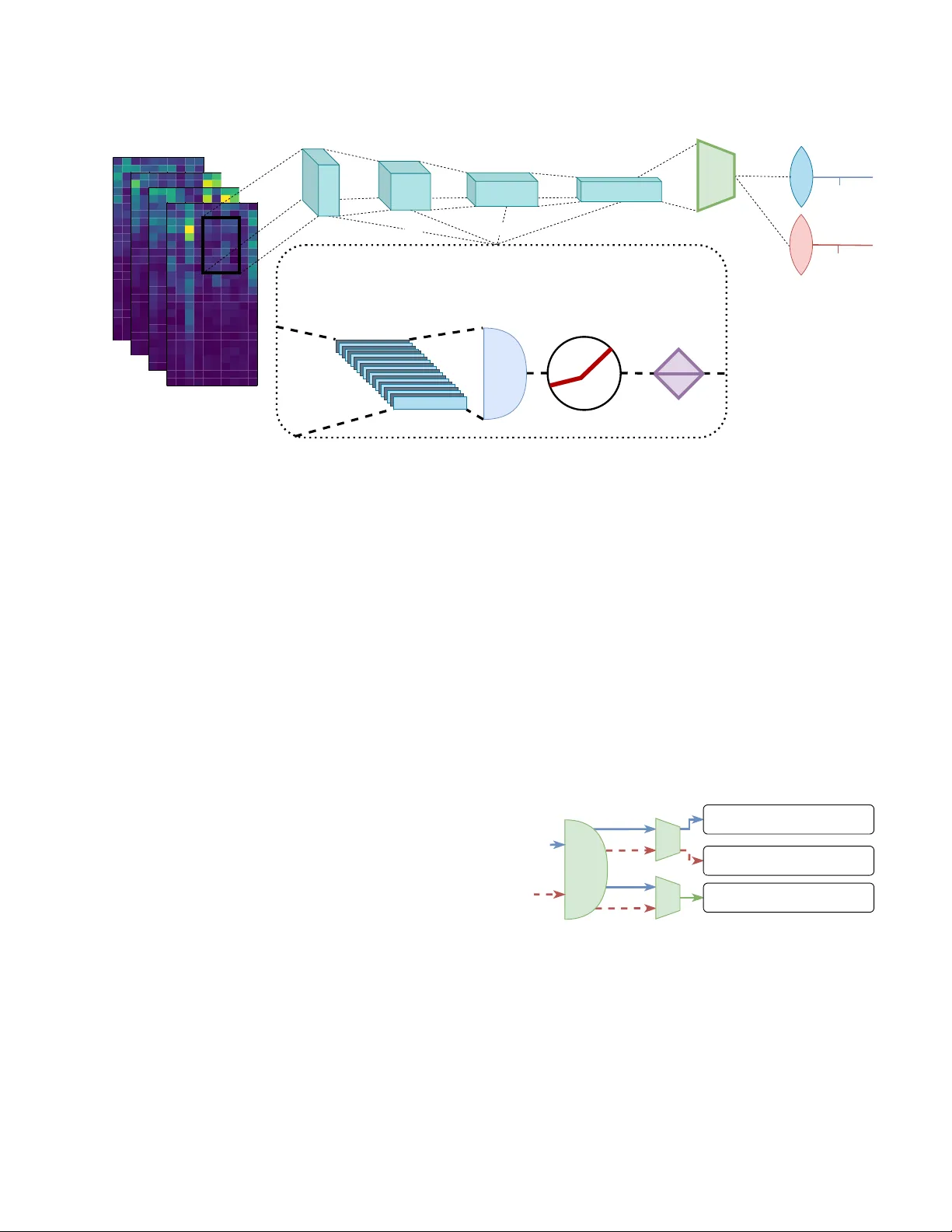
1 Unsupervised Domain Adv ersarial Self-Calibration for Electromyography-based Gesture Recognition Ulysse C ˆ ot ´ e-Allard, Gabriel Gagnon-T urcotte, Angkoon Phin yomark, K yrre Glette, Erik Scheme † , Franc ¸ ois Laviolette † , and Benoit Gosselin † Abstract —Surface electromy ography (sEMG) pr ovides an intu- itive and non-inv asive interface from which to control machines. Howev er , preser ving the myoelectric contr ol system’ s perfor - mance over multiple days is challenging, due to the transient nature of the signals obtained with this recording technique. In practice, if the system is to remain usable, a time-consuming and periodic recalibration is necessary . In the case where the sEMG interface is employed every few days, the user might need to do this r ecalibration bef or e e very use. Thus, sever ely limiting the practicality of such a control method. Consequently , this paper proposes tackling the especially challenging task of unsupervised adaptation of sEMG signals, when multiple days hav e elapsed between each recording, by introducing Self-Calibrating Asyn- chronous Domain Adversarial Neural Network (SCAD ANN). SCAD ANN is compared with two state-of-the-art self-calibrating algorithms developed speciﬁcally for deep learning within the context of EMG-based gesture recognition and three state-of-the- art domain adversarial algorithms. The comparison is made both on an ofﬂine and a dynamic dataset (20 participants per dataset), using two different deep network architectur es with two different input modalities (temporal-spatial descriptors and spectrograms). Overall, SCADANN is shown to substantially and systematically impro ves classiﬁcation performances over no recalibration and obtains the highest av erage accuracy for all tested cases across all methods. Index T erms —EMG, Myoelectric Contr ol, Domain Adaptation, Self-Calibration, Domain Adversarial, Gesture Recognition. I . I N T R O D U C T I O N Robots ha ve become increasingly prominent in the li ves of human beings. As a result, the way in which people interact with machines is constantly ev olving towards a better synergy between human intention and machine action. The ease of transcribing intention into commands is highly dependent on the type of interface and its implementations [1]. Within this context, muscle activity offers an attractiv e and intuiti ve way to perform gesture recognition as a guidance method [2], [3]. Such activity can be recorded from surface electromyography (sEMG), a non-in v asiv e technique widely adopted both for prosthetic control and in research as a way to seamlessly interact with machines [4], [5]. Artiﬁcial intelligence can then be lev eraged as the bridge between these biological signals and a robot’ s input guidance. Current state-of-the-art algorithms in gesture recognition routinely achie ve accuracies abo ve 95% for the classiﬁca- tion of ofﬂine, within-day datasets [6], [7]. Howe ver , many practical issues still need to be solved before implementing these types of algorithms into functional applications [4], [8]. † These authors share senior authorship Electrode shift and the transient nature of the sEMG signals are among the main obstacles to a robust and widespread imple- mentation of real-time sEMG-based gesture recognition [4]. In practice, this means that users of current myoelectric systems need to perform periodic recalibration of their device so as to retain their usability . T o address the issue of real-time myoelectric control, researchers have proposed rejection-based methods where a gesture is predicted only when a suf ﬁcient lev el of certainty is achieved [9], [10]. While this type of method have been sho wn to increase online usability , they do not directly address the inherent decline in performance of the classiﬁer over time. One way to tackle this challenge is to lev erage transfer learning algorithms to periodically recalibrate the system with less data than normally required [11], [12]. Though this reduces the burden placed on the user, said user will still need to periodically record new labeled data. This work focuses on the problem of across-day sEMG- based gesture recognition both within an ofﬂine and dynamic setting. In particular, this work considers the situation where sev eral days ha ve elapsed between each recording session. Such a setting naturally arises when sEMG-based gesture recognition is used for video games, artistic performances or , simply , to control devices of sporadic use [13], [5], [2]. In contrast to within-day or even day-to-day adaptation, this work’ s setting is especially challenging as the change in the signal between two sessions is expected to be substantially greater and no intermediary data is av ailable to bridge this gap. The goal is then for the classiﬁer to be able to adapt over -time using the unlabe led data obtained from the myoelectric system. Such a problem can be framed within an unsupervised domain adaptation setting [14] where there exists an initial labeled dataset on which to train, but the classiﬁer then has to adapt to unlabeled data from a different, but similar distribution. An additional dif ﬁculty of the setting considered in this work is that real-time myoelectric control imposes strict limi- tations in relation to the amount of temporal data which can be accumulated before each new prediction. The window’ s length requirement has a direct negati ve impact on the performance of classiﬁers [15], [10]. This is due to the fact that tempo- rally neighboring segments most likely belong to the same class [16], [17]. In other words, provided that predictions can be deferred, it should be possible to generate a classiﬁcation algorithm with impro ved accuracy (compared to the real- time classiﬁer) by looking at a wider temporal context of the data [10]. Consequently , one possibility to cope with electrode shift and the non-stationary nature of EMG signals for gesture recognition is for the classiﬁer to self-calibrate using pseudo- 2 labels generated from this improved classiﬁcation scheme. The most natural way of performing this relabeling is using a majority v ote around each classiﬁer’ s prediction. Xiaolong et al. [17] hav e shown that such a recalibration strategy signiﬁcantly improves intra-day accuracy on an ofﬂine dataset for both amputees and able-bodied subjects (tested on the NinaPro DB2 and DB3 datasets [18]). Howe ver for real-time control, such a majority vote strategy will increase latency , as transitions between gestures inevitably take longer to be detected. Additionally , as the domain div ergence, over multiple days, is expected to be substantially greater than within a single day , ignoring this gap before generating the pseudo- labels might negati vely impact the self-recalibrated classiﬁer . Finally , trying to re-label ev ery segment, ev en when there is no clear gesture detected by the classiﬁer , will necessarily introduce undesirable noise in the pseudo-labels. T o address these issues, the main contrib ution of this paper is the in- troduction of SCAD ANN (for Self-Calibrating Asynchronous Domain Adversarial Neural Network), a deep learning-based algorithm, which lev erages the domain adaptation setting and the unique properties of real-time myoelectric control for inter- day self-recalibration. This paper is org anized as follows. An overvie w of the related work is gi ven in Section II. The datasets and the deep network architecture employed in this work is provided in Section III. Section IV presents the domain adaptation algorithm considered in this work, while Section V thoroughly describes SCAD ANN alongside the two most popular sEMG- based unsupervised adaptation algorithms. Finally , these three algorithms are compared alongside the domain adaptation algorithms and the vanilla networks in Section VI and their associated discussions are sho wn in Section VII. I I . R E L A T E D W O R K Myoelectric control systems naturally generate large amounts of unlabeled data. Howe ver , ov er time, due to the electrode shift and transient change in the signal, the data generated div erges from the one used for training the classiﬁer . Huang et al. [19] proposes using this setting to update a modiﬁed Support V ector Machine, by replacing some of the key examples (referred to as representative particles (RP)) from the training set, with new unlabeled examples when they are sufﬁciently close (i.e. small distance within the feature space) to the RP . Other authors [20] propose to periodically retrain a Linear Discriminant Analysis (LD A), by updating the training dataset itself. The idea is to replace the oldest examples with new , near ones. Such methods, howe ver , are inherently restricted to single-day use as they rely on smooth and small signal drift to update the classiﬁer . Additionally , these types of methods do not leverage the potentially large quantity of unlabeled data generated. In contrast, deep learning algorithms are well suited to scale to lar ge amounts of data and were shown to be more robust to between-day signal drift than LD A, especially as the amount of training data increases [21]. W ithin the ﬁeld of image recognition, deep learning-based unsupervised domain adaptation has been extensiv ely studied. A popular approach to this problem is domain adversarial training popularized by D ANN [14], [22]. The idea behind D ANN is to learn a feature representation which fav ors class separability of the labeled dataset, while simultaneously hindering domain separability (i.e. differentiation between the labeled and unlabeled examples). See Section IV for details. Building on D ANN, the V AD A (for V irtual Adversarial Do- main Adaptation) algorithm [23] proposes to also minimize the cluster assumption violations on the unlabeled dataset [24] (i.e. decision boundary should av oid area of high data density). Another state-of-the-art algorithm, but this time for non- conservati v e unsupervised domain adaptation (i.e. the ﬁnal model might not be good at classifying the original data), is DIR T -T (for Decision-boundary Iterative Reﬁnement Training with a T eacher), which starting from the output of V AD A, remov es the labeled data and iterativ ely tries to continue minimizing the cluster assumption. A detailed explanation of D ANN, V AD A and DIR T -T is given in Section IV. These three state-of-the-art domain adversarial algorithms achiev e a two-digit accuracy increase on se veral difﬁcult image recog- nition benchmarks [23] compared to the non-adapted deep network. This work thus proposes to test these algorithms on the challenging problem of multiple-day sEMG-based gesture recognition both within an ofﬂine and dynamic setting (see Section VI). I I I . D A TA S E T S A N D N E T W O R K ’ S A R C H I T E C T U R E This work employs the 3DC Dataset [25] for architecture building and hyperparameter optimization and the Long-term 3DC Dataset [12] for training and testing the different al- gorithms considered. Both datasets were recorded using the 3DC Armband [25]; a wireless, 10-channel, dry-electrode, 3D printed sEMG armband. The device samples data at 1000 Hz per channel, allo wing to take adv antage of the full spectra of sEMG signals [26]. As stated in [25], [12], the data acquisition protocol of the 3DC Dataset and Long-term 3DC Dataset were approved by the Comit ´ es d’ ´ Ethique de la Recherche av ec des ˆ etres humains de l’Universit ´ e Laval (approv al number: 2017-0256 A-1/10- 09-2018 and 2017-026 A2-R2/26-06-2019 respectiv ely), and informed consent was obtained from all participants. A. Long-term 3DC Dataset The Long-term 3DC Dataset features 20 able-bodied partic- ipants (5F/15M) aged between 18 and 34 years old (av erage 26 ± 4 years old) performing elev en gestures (shown in Fig- ure 1). Each participant performed three recording sessions ov er a period of fourteen days (in sev en-day increments). Each recording session is divided into a T raining Recor ding and two Evaluation Recordings . For each new session, the participants were the ones placing the armband on their forearm at the beginning of each session (introducing small electrode shift between each session). The Long-term 3DC Dataset was recorded within a virtual reality environment in conjunction with the leap motion cam- era. The usefulness of the VR environment was three fold. First, it allowed to more intuitiv ely communicate requested gesture intensity and position to the participant. Second, it 3 allowed to replace the arm of the participant with a virtual pr osthetic , which provided direct and intuiti ve feedback (ges- ture held, intensity and position) to the participant. Third, it allowed the gamiﬁcation of the experimental protocol, which greatly facilitated both recruitment and participant retention. During recording, the leap motion, in conjunction with an image-based con volutional network, served as the real-time controller and as a way to provide feedback without biasing the dataset to a particular EMG-based classiﬁer . The dataset is thoroughly described alongside a detailed explanation of the VR system and the contributions of the leap motion camera in [12]. A brief overvie w of the dataset is provided in the following subsections. A video showing the recording protocol in action is also a vailable at the following link: https://www .youtube.com/watch?v=BnDwcw8ol6U. Neutral Radial Deviation Wrist Flexion Ulnar Deviation Wrist Extension Supination Pronation Power Grip Open Hand Chuck Grip Pinch Grip Reduced Gesture Dataset 2042.0000000000018 2042.0000000000018 Fig. 1. The elev en hand/wrist gestures recorded in the Long-term 3DC dataset and the 3DC Dataset . The gestures included within the Reduced Long-term 3DC Dataset are encompassed within the green line (7 gestures totals). 1) T raining Recor ding: During the T raining Recording, each participant was standing and held their forearm, unsup- ported, parallel to the ﬂoor , with their hand relaxed (neutral position). Starting from this neutral position, each participant was asked to perform and hold each gesture for a period of ﬁve seconds. This was referred to as a cycle . T wo more such cycles were recorded. In this work, the ﬁrst two cycles are used for training, while the last one is used for testing (unless speciﬁed otherwise). Note that in the original dataset, four cycles are recorded for each participant, with the second one recording the participant performing each gesture with maximal intensity . This second cycle was removed for this work to reduce confounding factors. In other words, cycle two and three in this work correspond to cycle three and four in the original dataset. In addition to the elev en gestures considered in the Long- term 3DC Dataset, a reduced dataset from the original Long- term Dataset containing sev en gestures is also employed. This Reduced Long-term 3DC Dataset is considered as it could more realistically be implemented on a real-world system giv en the current state of the art of EMG-based hand gesture recognition. The follo wing gestures form the reduced dataset: neutral, open hand, po wer grip, radial/ulnar deviation and wrist ﬂexion/e xtension. These gestures were selected as they were shown to be sufﬁcient in conjunction with orientation data to control a 6 degree-of-freedom robotic arm in real-time [2]. 2) Evaluation Recor ding: During the Evaluation Record- ings, the participants were asked to perform a speciﬁc gesture at a speciﬁc intensity (lo w , medium and high intensity based on their corresponding maximal gesture intensity) and at a random position (a point within reach of the participant’ s extended arm at a maximum angle of ± 45 and ± 70 degrees in pitch and yaw respecti vely). A ne w gesture, intensity and position were randomly asked ev ery ﬁve seconds. Each Evaluation Recording lasted three and a half minutes and two such recordings were performed by each participant for each recording session (total of six Evaluation Recordings per participant). The Evaluation Recordings provide a dynamic dataset which includes the transitions between the different gestures and the four main dynamic factors [4] (i.e. con- traction intensity , inter-day recording, electrode shifts and limb position) in sEMG-based gesture recognition. Note that while the participants recei ved visual feedback within the VR en vironment in relation to the held gesture, limb position and gesture intensity , the performed gestures were classiﬁed using the leap motion camera [27] in order to av oid bias in the dataset tow ards a particular EMG-based classiﬁer . In other words, the controller used by the participants during the Evaluation Recordings is distinct and independent from the sEMG-based gesture recognition algorithms considered in this manuscript, which is the main difference between the dynamic dataset considered and a real-time dataset. In this work, the ﬁrst ev aluation recording of a gi ven session was employed as the unlabeled training dataset for the algorithms presented in Section IV and V, while the second e valuation recording was used for testing. 3) Data Pre-pr ocessing: This work aims at studying un- supervised recalibration of myoelectric control systems. Con- sequently , the input latency is a critical factor to consider . The optimal guidance latency was found to be between 150 and 250 ms [15]. As such, the data from each participant is segmented into 150 ms frames with an overlap of 100 ms. Each segment thus contains 10 × 150 ( channel × time ) data points. The segmented data is then band-pass ﬁltered between 20-495 Hz using a fourth-order butterworth ﬁlter . Giv en a segment, the spectrogram for each sEMG channel are then computed using a 48 points Hann window with an ov erlap of 14 yielding a matrix of 4 × 25 ( time × f r eq uency ). The ﬁrst frequency band is then removed in an effort to reduce baseline drift and motion artifacts. Finally , following [28], the time and channel axis are swapped such that an example is of the shape 4 × 10 × 24 ( time × channel × f r eq uency ). Spec- trograms were selected as inputs for the Con vNet presented in Section III-C, as they hav e been sho wn to obtain competitive performance on a wide variety of datasets [6], [17], [25] and in the control of a robotic arm in real-time [2]. In addition, they are relatively inexpensiv e to compute and allow for faster training of a Con vNet when compared to the raw sEMG signal due to the relati vely low dimensionality of the obtained input images from the spectrograms. B. 3DC Dataset The 3DC Dataset features 22 able-bodied participants and is employed for architecture building and hyperparameter selection. This dataset, presented in [25], includes the same elev en gestures as the Long-term 3DC Dataset. Its recording 4 protocol closely matches the T raining Recording description (Section III-A), with the difference being that two such record- ings were taken for each participant (within the same day). This dataset was preprocessed as described in Section III-A3. C. Convolutional Network’s Arc hitectur e A small and simple Con vNet’ s architecture inspired from [29] and presented in Figure 2 was selected to reduce potential confounding factors. The ConvNet’ s architecture con- tains four blocks followed by a global av erage pooling and two heads. The ﬁrst head is used to predict the gesture held by the participant. The second head is only activ ated when employing domain adversarial algorithms (see Section IV and V for details). Each block encapsulates a con v olutional layer [30], followed by batch normalization [31], leaky ReLU [32] and dropout (set to p=0.5) [33]. AD AM [34] is employed for the Con vNet’ s optimization with batch size of 512. The learning rate (lr=0.001316) was selected with the 3DC Dataset by random search [35] using a uniform random distribution on a logarithmic scale between 10 − 5 and 10 1 and 100 candidates (each candidate was e val- uated 5 times). Early stopping, with a patience of 10 epochs, is also applied by using 10% of the training dataset as a validation set. Additionally , learning rate annealing, with a factor of ﬁv e and a patience of ﬁv e, was also used. W ithin this paper , this classiﬁer will be refered to as Spectrogram Con vNet. Note that the Con vNet’ s architecture implementation, writ- ten with PyT orch [36], is made readily av ailable here (https://github .com/UlysseCoteAllard/LongT ermEMG). D. T emporal-Spatial Descriptors Deep Network Due to the ubiquity of handcrafted feature sets within the ﬁeld of EMG-based gesture recognition, a deep network taking T emporal-Spatial Descriptors (TSD) as input is also considered. TSD is a handcrafted feature set proposed by Khushaba et al. [37] which achiev ed state-of-the-art results in EMG-based gesture classiﬁcation. A short ov ervie w of this feature set is giv en in Appendix A and the interested reader is encouraged to consult [37] for a detailed description. Note that before computing the gesture, the data is preprocessed as described in Section III-A3 (without the spectrogram part). The deep network architecture was again selected to be as simple as possible and is comprised of 3 fully connected layers each 200 neurons wide. Each layer also applies batch normalization, leak y ReLU (slope 0.1) as the activ ation func- tion and dropout (p=0.5). The training procedure is the same as for the Spectrogram Con vNet. AD AM is also employed with a learning rate of 0.002515 (found by cross-v alidation on the 3DC Dataset using the same hyperparameter as the Spectrogram Con vNet). The PyT orch implementation of the Deep Network, which will be referred to as TSD DNN for the remainder of this paper, is also made readily av ailable here (https://github .com/UlysseCoteAllard/LongT ermEMG). E. Calibration Methods This work considers three types of calibration for long-term classiﬁcation of sEMG signals: No Calibration, Recalibration and Unsupervised Calibration. In the ﬁrst case, the network is trained solely from the data of the ﬁrst session. In the Recalibration case, the model is re-trained at each new session with the new labeled data. Unsupervised Calibration is similar to Recalibration, but the dataset used for recalibration is unla- beled. Section IV and V presents the unsupervised calibration algorithms considered in this work. I V . U N S U P E RV I S E D D O M A I N A D A P TA T I O N Domain adaptation is an area in machine learning which aims at learning a discriminativ e predictor from two datasets (source and target datasets) coming from two different, but related, distributions [22] (referred to as D s and D t ). In the unsupervised case, one of the datasets is labeled (and comes from D s ), while the second is unlabeled (and comes from D t ). W ithin the context of myoelectric control systems, labeled data is obtained through a user’ s conscious calibration session. Howe v er , due to the transient nature of sEMG signals [4], [38], classiﬁcation performance tends to degrade over time. This naturally creates a burden for the user who needs to periodi- cally recalibrate the system to maintain its usability [38], [39]. During normal usage, howe ver , unlabeled data is constantly generated. Consequently , the unsupervised domain adaptation setting naturally arises by deﬁning the sour ce dataset as the labeled data of the calibration session and the targ et dataset as the unlabeled data generated by the user during control. The PyT orch implementation of the domain adversarial algorithms is mainly based on [40]. A. Domain-Adversarial T raining of Neural Networks The Domain-Adversarial Neural Network (D ANN) algo- rithm proposes to predict on the target dataset by learning a representation from the source dataset that makes it hard to distinguish examples from either distribution [14], [22]. T o achiev e this objective, DANN adds a second head (which may be comprised of one or more layers) to the network. This head, referred to as the domain classiﬁcation head , receives the features from the last feature extraction layer of the network (in this work case; from the global av erage pooling layer). The goal of this second head is to learn to discriminate between the two domains (source and target). Howe ver , during back- propagation, the gradient computed from the domain loss is multiplied by a negati ve constant (-1 in this work). This gradi- ent rev ersal explicitly forces the feature distribution of the do- mains to be similar . The backpropagation algorithm proceeds normally for the original head (classiﬁcation head). The two losses are combined as follows: L y ( θ ; D s ) + λ d L d ( θ ; D s , D t ) , where θ is the classiﬁer’ s parametrization, L y and L d are the prediction and domain loss respectiv ely . λ d is a scalar that weights the domain loss (set to 0 . 1 in this work). B. Decision-boundary Iterative Reﬁnement T raining with a T eacher Decision-boundary Iterativ e Reﬁnement Training with a T eacher (DIR T -T) is a two-step domain-adversarial training 5 Spectrograms Input Example 4x10x24 Leaky ReLU slope=0.1 Bi, i ∈ {0,1,2,3} Conv {16,32,64,128} @{4x7, 3x7, 3x7, 3x6} Batch Norm Dropout p=0.5 Gesture Output 1 1 Softmax Global Average Pooling 64 32x5x12 64x5x6 128x3x1 16x7x18 B0 B1 B2 B3 Softmax Domain Output 2 Fig. 2. The ConvNet’ s architecture employing 206 548 learnable parameters. In this ﬁgure, B i refers to the ith block ( i ∈ { 0 , 1 , 2 , 3 } ). Con v refers to a con volutional layer . When working with the reduced dataset, the number of output neurons from the gesture-head are reduced to seven. algorithm which achiev es state-of-the-art results on a variety of domain adaptation benchmarks [23]. 1) Fir st step: During the ﬁrst step, referred to as V AD A (for V irtual Adversarial Domain Adaptation) [23]), training is done using D ANN as described previously (i.e. using a second head to discriminate between domains). Ho wev er , with V AD A, the network is also penalized when it violates the cluster assumption on the target. This assumption states that data belonging to the same cluster in the feature space share the same class. Consequently , decision boundaries should av oid crossing dense regions. As shown in [41], this behavior can be achiev ed by minimizing the conditional entropy with respect to the target distribution: L c ( θ ; D t ) = E x ∼D t  h θ ( x ) T ln( h θ ( x ))  (1) Where θ is the parametrization of a classiﬁer h . In practice, L c must be estimated from the av ailable data. Howe v er , as noted by [41], such an approximation breaks if the classiﬁer h is not locally-Lipschitz (i.e. an arbitrary small change in the classiﬁer’ s input produces an arbitrarily large change in the classiﬁer’ s output). T o remedy this, V AD A pro- poses to explicitly incorporate the locally-Lipschitz constraint during training via V irtual Adversarial T raining (V A T) [42]. V A T generates new ”virtual” examples at each training batch by applying small perturbation to the original data. The av er- age maximal Kullback-Leibler diver gence ( D KL ) [43] is then minimized between the real and virtual examples to enforce the locally-Lipschitz constraint. In other words, V A T adds the following function to minimize during training: L v ( θ ; D ) = E x ∼D  max || r ||≤  D KL ( h θ ( x ) || h θ ( x + r ))  (2) As V A T can be seen as a form of regularization, it is also applied for the source data. In summary , the combined loss function to minimize during V AD A training is: min θ L y ( θ ; D s ) + λ d L d ( θ ; D s , D t ) + λ v s L v ( θ ; D s )+ λ v t L v ( θ ; D t ) + λ c L c ( θ ; D t ) (3) Where the importance of each additional loss function is weighted with a hyperparameter ( λ d , λ v s , λ v t , λ c ) . A diagram of V AD A is provided in Figure 3. {x s ,y s } {x t } Domain Divergence Cross-Entropy + V A T Conditional Entropy + V A T Features Extraction Domain head Classiﬁcation head Fig. 3. The V ADA algorithm which simultaneously tries to reduce the div ergence between the labeled source ( { x s , y s } ) and unlabeled target ( { x t } ) dataset while also penalizing violation of the cluster assumption on the target dataset. 2) Second Step: During the second step, the signal from the source is removed. The idea is then to ﬁnd a ne w parametriza- tion that further minimizes the target cluster assumption vio- lation while remaining close to the classiﬁer found during the ﬁrst step. This process can then be repeated by updating the original classiﬁer with the classiﬁer’ s parametrization found at 6 each iteration. The combined loss function to minimize during the n th iteration thus becomes: min θ n β E  D KL ( h θ n − 1 ( x ) || h θ n ( x ))  + λ v t L v ( θ ; D t ) + λ c L c ( θ ; D t ) (4) Where β is a hyperparameter which weighs the importance of remaining close to h θ n − 1 . In practice, the optimization prob- lem of Eq. 4 can be approximately solved with a ﬁnite number of stochastic gradient descent steps [23]. Following [23], the hyperparameters values are set to λ d = 10 − 2 , λ v s = 1 , λ v t = 10 − 2 , λ c = 10 − 2 , β = 10 − 2 . Note that, both D ANN and V AD A were conservati ve do- main adaptation algorithms (i.e. the training algorithms try to generate a classiﬁer that is able to discriminate between classes from both the source and target simultaneously). In contrast, DIR T -T is non-conservati ve as it ignores the source’ s signal during training. In the case where the gap between the source and the target is important, this type of non-conservati ve algorithm is expected to perform better than its conservati ve counterparts [23]. C. Unsupervised Adaptation - Hyperparameters Selection One challenge in applying unsupervised domain adaptation algorithms is the selection of the hyperparameters associated with the loss functions’ weights. This is due to the absence of labeled data on the target dataset, which in practice prohibits performing standard hyperparameter selection. One possible solution is to perform the adaptation without explicitly min- imizing the distance between the source and target, so that this distance can be used as a measure of adaptation perfor- mance [44]. Howe ver , such a solution precludes algorithms like the ones considered in this work and so the question of how to best perform hyperparameters selection remains a difﬁcult and open question. In their work introducing V AD A and DIR T -T [23], Shu et al. observed that extensiv e hyperparameter tuning was not necessary to achiev e state-of-the-art performance on the datasets they were using. Consequently , following this obser- vation, the hyperparameters associated with the unsupervised domain adversarial algorithms described in this section used the defaults weights recommended in their respectiv e paper . V . U N S U P E RV I S E D S E L F - C A L I B R AT I O N W ithin an unsupervised domain adaptation setting, the clas- siﬁer’ s performance is limited by the unav ailability of labeled data from the target domain. Howe ver , real-time EMG-based gesture recognition offers a particular situation from which pseudo-labels can be generated from the recorded data by looking at the prediction’ s context. These pseudo-labels can then be used as a way for the classiﬁer to perform self- recalibration. Zhai et al. [17] proposed to le verage this context by relabeling the network’ s predictions. Let P ( i, j ) be the softmax value of the network’ s output for the j th gesture (associated with the j th output neuron) of the i th example of a sequence. The heuristic considers an array composed of the t segments surrounding example i (included). For each j , the median softmax v alue ov er this array is computed: ˜ P ( i, j ) = median ( P ( i − t, j ) , P ( i − t + 1 , j ) , ..., P ( i, j ) , ..., P ( i + t, j )) (5) The pseudo-label of i then becomes the gesture j associated with the maximal ˜ P ( i, j ) . The median of the softmax’ s outputs is used instead of the prediction’ s mean to reduce the impact of outliers [17]. This self-calibrating heuristic will be referred to as MV (for Multiple V otes) from now on. As it was the best performing setting, the All-Session recalibration setting (i.e. using all a vailable unlabeled data across sessions) [17] is employed for MV . The hyperparameter t was set to 1 second, as recommended in [17]. This work proposes to improve on MV with a new self- calibrating algorithm, named SCADANN, which can be di- vided into three steps: 1) Apply D ANN to the network using the labeled and newly acquired unlabeled data. 2) Using the adapted network, perform the relabeling scheme described in Section V -A. 3) Starting from the adapted network, train the network with the pseudo-labeled data and labeled data while con- tinuing to apply D ANN to minimize domain di vergence. The ﬁrst step aims at reducing the domain di vergence be- tween the labeled recording session and the unlabeled record- ing to improv e classiﬁcation performance of the network. The second step uses the pseudo-labeling heuristic described in Section V -A. In addition to using the prediction’ s context to enhance the relabeling process, the proposed heuristic introduces two improvements compared to [17]: First, the heuristic tries to detect transition from one gesture to another . Then, already relabeled predictions falling within the transition period are vetted and possibly relabeled to better reﬂect when the actual transition occurred. This improvement aims at addressing two problems. First, the added latency introduced by majority-voting pseudo-labeling is remov ed. Second, this relabeling can provide the training algorithm with gesture transition examples. This is of particular interest as labeled transition examples are simply too time consuming to produce, especially considering the current need for periodic recalibration ( g gestures create g × ( g − 1) transitions to record). Introducing pseudo-labeled transition examples within the target dataset, could allow the network to detect transitions more rapidly and thus reduce the system latenc y . In turn, due to this latency’ s reduction, windo w’ s length could be increases to improv e the ov erall system’ s performance. The second improv ement, introduces the notion of stability to the network’ s predictions. Using this notion, the heuristic remov es e xamples that are more likely to be relabeled falsely from the pseudo-labeled dataset. This second improv ement is essential for a realistic implementation of self-calibrating algo- rithms, as otherwise the pseudo-labeled dataset would rapidly be ﬁlled with an important quantity of noise. This would result in a rapidly degenerating network as self-calibration is performed iterati vely . 7 The third step re-calibrates the network using the labeled and pseudo-labeled dataset in conjunction. D ANN is again employed to try to obtain a similar feature representation between the source and target datasets. The source dataset contains the labeled dataset alongside all the pseudo-labeled data from prior sessions, while the target dataset contains the pseudo-labeled data from the current session. The dif ference with SCAD ANN’ s ﬁrst step is that the network’ s weights are also optimized in relation to the cross-entropy loss calculated from the newly generated pseudo-labels. If only the pseudo- labeled dataset was employed for recalibration, the network performance would rapidly degrade from being trained only with noisy labels and possibly without certain gestures (i.e. nothing ensure that the pseudo-labeled dataset is balanced or ev en contains all the gestures). Early stopping is performed using part of the ne wly generated pseudo-labels. A. Proposed Pseudo-labels Generating Heuristic For concision’ s sake, the pseudo-code for the proposed rela- beling heuristic is presented in Appendix B-Algorithm 1. Note also that a python implementation of SCADANN (alongside the pseudo-labeling heuristic) is a vailable in the previously mentioned online repository. The main idea behind the heuristic is that if the ne w pre- diction is different than the previous one, the state goes from stable to unstable . During the stable state, the prediction of the considered segment is added to the pseudo-label array . During the unstable state, all the network’ s output (after the softmax layer) are instead accumulated in a second array . When this second array contains enough segments (hyperparameter sets to 1.5s), the class associated with the output neuron with the highest median value is deﬁned as the ne w possible stable class. The new possible stable class is conﬁrmed if the median percentage of this class (compared with the other classes) is abov e a certain threshold (85% and 65% for the seven and elev en gestures dataset respectiv ely (selected using the 3DC dataset)). If this threshold is not achiev ed, the oldest element in the second array is removed and replaced with the next element. Note that the computation of the new possible stable class using the median is identical to MV . When the new possible class is conﬁrmed, the heuristic ﬁrst veriﬁes if it was in the unstable state for too long (2s in this work). If it was, all the predictions accumulated during the unstable state are removed. Otherwise, if the ne w stable state class is different than before it means that a gesture’ s transition probably occurred. Consequently , the heuristic goes back in time before the instability began (maximum of 0.5s in this work) and looks at the deriv ati ve of the entropy calculated from the network’ s softmax output to determine when the network started to be affected by the gesture’ s transition. All the segments from this instability period (and adding the relev ant segments from the look-back step) are then relabeled as the new stable state class found. If instead the ne w stable state class is identical to the previous one, only the segments from the instability period are relabeled. The heuristic then returns to its stable state. B. SCADANN - Hyperparameters Selection On the surface, SCAD ANN introduces sev eral hyperpa- rameters whose selection, within an unsupervised domain adaptation paradigm, is not straightforward. The majority of the introduced hyperparameters, howe ver , have a meaningful interpretation within the context of EMG-based gesture recog- nition. In other words, reasonable values can be assigned to them without performing detailed data-driven hyperparameter selection. In addition, because these newly introduced hyper- parameters are solely related to the pseudo-labeling aspect of the work, a labeled dataset (in this work case the 3DC Dataset) can be le veraged to perform hyperparameter selection. C. Adaptive Batch Normalization For the sake of completeness, in addition to the ﬁ ve previously mentioned adaptation algorithms, this work also considers Adaptiv e Batch Normalization (AdaBN) [45], [39]. AdaBN is an unsupervised domain adaptation algorithm which was successfully applied to EMG-based gesture recognition in [39]. The hypothesis behind AdaBN is that the label- related information (the difference between gestures) can be encapsulated within the weights of the network, while the domain-related information (the difference between sessions) are contained within the batch normalization (BN) statistics. In practice, this means that the adaptation is done by feeding the unlabeled examples from the target dataset to the network to update the BN statistics. Note that within this work’ s setting, as only one session is contained within the source dataset and inter-user classiﬁcation is not considered, the multi-stream aspect proposed in [39] cannot be applied. V I . E X P E R I M E N T S A N D R E S U LT S As suggested in [46], a two-step statistical procedure is used whenev er multiple algorithms are compared against each other . First, Friedman’ s test ranks the algorithms amongst each other . Then, Holm’ s post-hoc test is applied ( n = 20 ) using the No Calibration setting as a comparison basis. Additionally , Cohen’ s D z [47] is employed to determine the effect size of using one of the self-supervised algorithm over the No Cali- bration setting. T o better contextualize the performance of the basic Spectrogram Con vNet used in this work, a comparison between the Spectrogram Con vNet and 6 widely used features ensembles within the ﬁeld of sEMG-based gesture recognition is performed. For the sake of concision, this comparison is giv en in Appendix A. A. T raining Recor ding In this subsection, all training was performed using the ﬁrst and second cycles of the relev ant T raining Recording, while the third cycle was employed for testing. All 20 participants completed three Training Recordings and only the labels from the ﬁrst Training Recording are used (the data from the other T raining Recordings are used without labels for the unsupervised recalibrations algorithms when relev ant). The time-gap between each Training Recording was around se ven days (14-day gap between session 1 and 3). Note that for the ﬁrst session, all algorithms are equiv alent to the No Calibration scheme and consequently perform the same. 8 1) Ofﬂine Seven Gestures Reduced Dataset: T able I shows a comparison of the No Calibration setting alongside the three D A algorithms, AdaBN, MV and SCAD ANN for both the Spectrogram Con vNet and the TSD DNN. T ABLE I O FFL I N E A C C U R A C Y F O R S E V E N G E S T U R E S Spectrogram Con vNet No Cal DANN V ADA Dirt-T AdaBN MV SCADANN Session 0 STD 93.58% 4.58% N \ A N \ A N \ A N \ A N \ A N \ A N \ A N \ A N \ A N \ A N \ A N \ A Session 1 STD Friedman Rank H0 Cohen’ s Dz 71.10% 22.90% 4.85 N \ A N \ A 72.76% 26.00% 4.73 1 0.19 73.35% 25.48% 4.25 1 0.24 74.28% 24.42% 3.70 1 0.36 72.61% 25.95% 5.23 1 0.16 74.45% 24.03% 2.78 0 (0.01193) 0.62 75.50% 25.41% 2.48 0 (0.00305) 0.52 Session 2 STD Friedman Rank H0 Cohen’ s Dz 68.75% 22.58% 5.60 N \ A N \ A 74.49% 22.73% 4.40 1 0.73 75.55% 22.76% 4.03 1 0.77 75.52% 23.55% 3.40 0 (0.00512) 0.70 76.02% 23.10% 2.95 0 (0.00063) 0.79 70.01% 24.82% 4.68 1 0.22 77.22% 22.50% 2.95 0 (0.00063) 0.92 TSD DNN No Cal DANN V ADA Dirt-T AdaBN MV SCADANN Session 0 STD 96.39% 3.20% N \ A N \ A N \ A N \ A N \ A N \ A N \ A N \ A N \ A N \ A N \ A N \ A Session 1 STD Friedman Rank H0 Cohen’ s Dz 78.14% 18.49% 5.45 N \ A N \ A 83.15% 15.47% 4.03 1 0.90 80.90% 15.46% 4.95 1 0.37 80.94% 14.06% 4.68 1 0.22 84.37% 14.64% 3.00 0 (0.00168) 0.88 83.01% 19.43% 3.48 0 (0.01536) 0.86 84.91% 16.09% 2.43 0 (0.00006) 0.84 Session 2 STD Friedman Rank H0 Cohen’ s Dz 79.78% 19.06% 5.20 N \ A N \ A 84.73% 19.38% 3.93 1 0.55 84.50% 17.37% 4.20 1 0.52 82.16% 17.68% 5.18 1 0.28 85.91% 19.06% 3.23 0 (0.01919) 0.61 81.47% 19.23% 4.15 1 0.48 88.20% 17.55% 2.13 0 (0.00004) 0.81 2) Ofﬂine Eleven Gesture Dataset: T able II compares the No Calibration setting with the three DA algorithms, AdaBN, MV and SCAD ANN for both networks. Figure 4 shows a histogram of the accuracy obtained by the TSD DNN for the No Calibration, SCAD ANN and the Recalibration methods. T ABLE II O FFL I N E A C C U R A C Y F O R E L E V E N G E S T U R E S Spectrogram ConvNet No Cal DANN V ADA Dirt-T AdaBN MV SCADANN Session 0 STD 84.19% 9.12% N \ A N \ A N \ A N \ A N \ A N \ A N \ A N \ A N \ A N \ A N \ A N \ A Session 1 STD Friedman Rank H0 Cohen’ s Dz 58.29% 25.33% 5.50 N \ A N \ A 62.27% 24.86% 3.85 0 (0.04626) 0.63 62.45% 25.00% 3.83 0 (0.04626) 0.63 62.35% 24.99% 3.78 0 (0.04626) 0.57 61.83% 25.42% 4.05 0 (0.04626) 0.49 60.75% 26.38% 3.55 0 (0.02155) 0.93 63.00% 24.84% 3.45 0 (0.01615) 0.71 Session 2 STD Friedman Rank H0 Cohen’ s Dz 56.69% 23.04% 5.43 N \ A N \ A 62.08% 22.84% 3.95 1 0.75 62.40% 22.77% 3.65 0 (0.04684) 0.77 62.43% 22.69% 3.68 0 (0.04684) 0.75 62.49% 22.98% 3.80 1 0.78 58.27% 23.26% 4.45 1 0.53 63.43% 23.03% 3.05 0 (0.00305) 0.68 TSD DNN No Cal DANN V ADA Dirt-T AdaBN MV SCADANN Session 0 STD 89.95% 8.37% N \ A N \ A N \ A N \ A N \ A N \ A N \ A N \ A N \ A N \ A N \ A N \ A Session 1 STD Friedman Rank H0 Cohen’ s Dz 66.16% 22.66% 5.65 N \ A N \ A 72.44% 20.58% 3.83 0 (0.02265) 0.76 69.25% 19.51% 4.75 1 0.36 69.14% 16.64% 4.88 1 0.26 73.63% 19.79% 3.18 0 (0.00146) 0.87 71.34% 23.41% 3.33 0 (0.00266) 0.92 75.40% 20.06% 2.40 0 (0.00001) 1.10 Session 2 STD Friedman Rank H0 Cohen’ s Dz 66.84% 20.53% 6.15 N \ A N \ A 74.30% 20.57% 4.13 0 (0.00607) 0.82 73.61% 18.65% 3.75 0 (0.00177) 0.71 73.71% 17.26% 3.95 0 (0.00384) 0.63 74.99% 21.97% 2.98 0 (0.00002) 0.80 69.94% 20.19% 4.70 0 (0.03379) 1.02 77.65% 19.52% 2.35 0 ( < 0.00001) 1.12 B. Evaluation Recording 1) Eleven Gestures - Dynamic Dataset, ofﬂine adaptation: T able III compares the No Calibration setting with the three D A algorithms, AdaBN, MV and SCAD ANN for both net- works on the second Ev aluation Recording of each session, when the labeled and unlabeled data lev eraged for training comes from the T raining Recordings (as in Section VI-A2). 2) Eleven Gestur es - Adaptation on the Dynamic Dataset: T able IV presents the comparison between the No Calibration setting and using the ﬁrst Evaluation Recording of each experiment’ s session as the unlabeled dataset for the three DA algorithms, AdaBN, MV and SCAD ANN.                  Fig. 4. Ofﬂine accuracy using the TSD DNN for the elev en gestures in respect to time. The values on the x-axis represent the a verage number of days elapsed across participants since the ﬁrst session. T ABLE III D Y N A M I C D A TAS E T ’ S AC C U R AC Y F O R E L E V E N G E S T U R E S U S I N G T R A I N I N G R E C O R D I N G S A S U N L A B E L E D DAT A Spectrogram ConvNet No Cal D ANN V ADA Dirt-T AdaBN MV SCAD ANN Session 0 STD 47.81% 10.94% N \ A N \ A N \ A N \ A N \ A N \ A N \ A N \ A N \ A N \ A N \ A N \ A Session 1 STD Friedman Rank H0 Cohen’ s Dz 38.39% 16.65% 4.80 N \ A N \ A 39.64% 17.37% 3.78 1 0.45 39.52% 17.66% 4.10 1 0.32 39.07% 17.56% 4.70 1 0.16 38.99 17.16% 4.33 1 0.17 39.70% 17.75% 3.30 1 0.54 40.80% 17.77% 3.00 1 0.63 Session 2 STD Friedman Rank H0 Cohen’ s Dz 38.54% 14.65% 5.50 N \ A N \ A 39.87% 15.32% 4.20 1 0.33 40.07% 15.81% 3.60 0 (0.02166) 0.35 39.59% 15.43% 4.45 1 0.25 39.53% 15.59% 4.30 1 0.22 40.98% 15.18% 3.35 0 (0.00824) 0.84 42.26% 16.34% 2.60 0 (0.00013) 0.65 TSD DNN No Cal D ANN V ADA Dirt-T AdaBN MV SCAD ANN Session 0 STD 53.08% 11.48% N \ A N \ A N \ A N \ A N \ A N \ A N \ A N \ A N \ A N \ A N \ A N \ A Session 1 STD Friedman Rank H0 Cohen’ s Dz 46.09% 14.70% 4.50 N \ A N \ A 48.07% 14.59% 3.00 1 0.55 43.92% 13.45% 5.40 1 -0.37 42.75% 12.65% 5.80 1 -0.49 47.11% 14.11% 3.75 1 0.21 48.36% 14.30% 2.85 1 1.08 49.09% 14.68% 2.70 1 0.67 Session 2 STD Friedman Rank H0 Cohen’ s Dz 46.01% 15.72% 4.90 N \ A N \ A 48.50% 15.80% 3.85 1 0.50 45.69% 14.21% 4.80 1 -0.05 45.48% 13.26% 5.00 1 -0.08 48.35% 16.17% 3.73 1 0.42 48.17% 17.06% 3.78 1 0.60 50.90% 16.64% 1.95 0 (0.00009) 0.91 A histogram of the dynamic dataset’ s accuracy of the No Calibration, Recalibrated, SCAD ANN and Recalibrated SCAD ANN methods, trained on the TSD DNN, using the ﬁrst Ev aluation Recording of each experimental session as unlabeled data is sho wn in Figure 5. The Recalibration SCAD ANN scheme systematically and signiﬁcantly (p < 0.05) outperforms the Recalibration scheme for all three sessions for both networks, using the Wilcoxon signed rank-test [48], [46], as can be seen from T able V. V I I . D I S C U S S I O N The task of performing adaptation when multiple days hav e elapsed is especially challenging. As a comparison, on the within-day adaptation task presented in [17], MV was able to enhance classiﬁcation accuracy by 10% on av erage compared to the No Calibration scheme. W ithin this work ho wev er , the greatest improvement achieved by MV was 3.35% for the Spectrogram Con vNet and 5.18% for the TSD DNN. Overall, the best improv ement in this paper was 8.47% and 10.81% both achie ved by SCADANN with the Spectrogram Con vNet and TSD DNN respectively . All three tested domain 9 T ABLE IV D Y N A M I C D A TAS E T ’ S AC C U R AC Y F O R E L E V E N G E S T U R E S U S I N G T H E FI R S T E V A L UATI O N R E C O R D I N G A S U N L A B E L E D D A TA Spectrogram ConvNet No Cal DANN V ADA Dirt-T AdaBN MV SCADANN Session 0 STD Friedman Rank H0 Cohen’ s Dz 47.81% 10.94% 4.75 N \ A N \ A 49.37% 11.24% 3.80 1 0.64 49.36% 11.04% 3.78 1 0.60 49.48% 11.21% 3.38 1 0.53 47.33% 10.45% 4.95 1 -0.11 47.68% 11.27% 4.80 1 -0.07 49.89% 11.25% 2.55 0 (0.00490) 0.73 Session 1 STD Friedman Rank H0 Cohen’ s Dz 38.39% 16.65% 5.15 N \ A N \ A 40.92% 18.51% 3.10 0 (0.02643) 0.56 40.73% 18.55% 3.63 1 0.53 40.66% 18.38% 3.85 1 0.49 40.36% 17.77% 4.25 1 0.41 38.60% 17.13% 4.83 1 0.13 41.07% 19.11% 3.20 0 (0.02643) 0.52 Session 2 STD Friedman Rank H0 Cohen’ s Dz 38.54% 14.65% 5.10 N \ A N \ A 40.78% 16.05% 2.78 0 (0.00063) 0.50 40.82% 16.05% 3.28 0 (0.00266) 0.48 41.01% 16.29% 2.95 0 (0.00063) 0.51 38.15% 15.36% 5.60 1 -0.07 40.02% 15.42% 4.10 1 0.79 41.41% 16.45% 3.50 0 (0.00633) 0.48 TSD DNN No Cal DANN V ADA Dirt-T AdaBN MV SCADANN Session 0 STD Friedman Rank H0 Cohen’ s Dz 53.08% 11.48% 4.10 N \ A N \ A 55.29% 12.09% 2.60 1 0.71 50.42% 10.67% 5.80 1 -0.81 53.59% 11.51% 4.00 1 0.13 49.98% 10.90% 5.50 1 -0.60 53.67% 11.51% 3.70 1 0.30 55.69% 12.37% 2.30 1 0.67 Session 1 STD Friedman Rank H0 Cohen’ s Dz 46.09% 14.70% 5.50 N \ A N \ A 50.65% 14.55% 2.30 0 (0.00001) 1.35 46.10% 13.66% 5.55 1 < 0.01 49.30% 13.81% 3.50 0 (0.01366) 0.73 48.12% 14.14% 4.60 1 0.36 47.34% 16.16% 4.40 1 0.46 51.41% 15.46% 2.15 0 (0.00001) 1.17 Session 2 STD Friedman Rank H0 Cohen’ s Dz 46.01% 15.72% 5.40 N \ A N \ A 50.91% 15.88% 2.65 0 (0.00028) 0.98 48.33% 14.12% 4.20 1 0.46 50.27% 14.60% 3.15 0 (0.00396) 0.84 44.22% 14.58% 5.90 1 -0.28 46.90% 16.31% 4.50 1 0.37 52.01% 17.17% 2.20 0 (0.00002) 1.32                     Fig. 5. TSD DNN dynamic dataset’ s accuracy for ele ven gestures in respect to time. Training is performed ofﬂine with the ﬁrst T raining Recording session. Adaptation takes place on the ﬁrst Evaluation Recording of the corresponding tested session, while the test set comes from the second Evaluation Recording of the same tested session. The values on the x-axis represent the a verage number of days elapsed across participants since the ﬁrst session. adversarial algorithms were also able to consistently improve the netw ork’ s accuracy compared to the No Calibration scheme (the only exception being V AD A and Dirt-T for the TSD DNN in T able III). When used to adapt to dynamic unsupervised data, some were even able to achiev e a higher ov erall ranking than SCAD ANN using the Spectrogram ConvNet. Note ho w- ev er , that the improv ements they seem to allo w is o verall lo wer than when they are applied on image-based dataset such as MNIST and CIF AR [23]. Deep domain adversarial algorithms thus seems to be a promising avenue to explore further , by dev eloping adversarial algorithms speciﬁcally for the ﬁeld of sEMG-based gesture recognition. SCAD ANN could then easily be augmented by these new algorithms to improve T ABLE V A C C U R A C Y F O R T H E Recalibration A N D Recalibration SCADANN W I T H E L E V E N G E S T U R E S O N T H E DY NA M I C DAT A S E T U S I N G T H E FI R S T E V A L U ATI O N R E C O R D I N G A S U N L A B E L E D DAT A Spectrogram ConvNet TSD DNN Recalibration Recalibration SCAD ANN Recalibration Recalibration SCAD ANN Session 0 STD H0 Cohen’ s Dz 47.81% 10.94% 0 (0.00642) N \ A 49.89% 11.25% 0 (0.00642) 0.73 53.08% 11.48% 0 (0.01000) N \ A 55.69% 12.37% 0 (0.01000) 0.67 Session 1 STD H0 Cohen’ s Dz 49.54% 11.28% 0 (0.00455) N \ A 53.02% 11.18% 0 (0.00455) 0.88 53.51% 11.98% 0 (0.00014) N \ A 58.34% 11.82% 0 (0.00014) 1.25 Session 2 STD H0 Cohen’ s Dz 52.18% 10.66% 0 (0.00059) N \ A 55.19% 10.15% 0 (0.00059) 1.11 57.18% 11.12% 0 (0.00012) N \ A 60.81% 10.10% 0 (0.00012) 0.75 *W ilcoxon signed rank test. Null hypothesis rejected when H0=0 (p < 0.05). performance further . In T able IV, it can be seen that the performances of MV dropped substantially compared to the other experiments conducted within this paper . A possible explanation is that this was the ﬁrst time that MV had to adapt using the Dynamic Dataset data. In other words, instead of adapting to a well deﬁned series of examples grouped by gesture, MV had to contend with a continuous data stream including gesture tran- sitions. In contrast, SCAD ANN actually performed generally better in T able IV than in T able III, which is encouraging as T able IV showcased a more realistic setting for unsupervised recalibration. It is also important to note that both the general performance and the type of error that the classiﬁer makes can greatly affect the self-calibrating algorithms. While SCADANN partially address the ﬁrst consideration (by ignoring data that are more likely to be misclassiﬁed), the second consideration is harder to address. That is, when the classiﬁer is not only wrong, but is conﬁdent in its error and that error spans over a large amount of time, the pseudo-labeling heuristic cannot hope to re-label the segments correctly or ev en identify this segment of data as problematic. In an effort to address this issue, future works could explore the use of a hybrid IMU/EMG system, as they hav e been sho wn to improve gesture recognition accuracy [49], [50]. The use of accelerometer data within the ﬁeld is generally linked with mechanomyogram (MMG), which is strongly associated with EMG signals. Recent works [51] ho wev er , hav e sho wn that, within a human-computer interaction con- text, accelerometer data can also help recognize different gestures with high accuracy using the positional variance of the different gestures, which is uncharacteristic of MMG. The fusion of these two different modalities could reduce the likelihood of concurrent errors, enabling SCADANN’ s rela- beling heuristic to generate the pseudo-labels more accurately . Note that, using EMG signals alone, SCAD ANN’ s relabeling heuristic substantially enhanced the pseudo-labels accuracy compared to the one used with MV . As an example, consider the supervised Recalibrating classiﬁer (with the Spectrogram Con vNet) trained on all the training cycles of the rele v ant T raining Recording and tested on the Evaluation Recording. This classiﬁer achiev es an av erage accuracy of 49.84% over 544 263 examples. In comparison, the MV relabeling heuristic 10 achiev es 54.28% accuracy ov er the same number of examples, while the SCAD ANN relabeling heuristic obtains 61.89% and keeps 478 958 examples using the 65% threshold. When using a threshold of 85%, the accuracy reaches 68.21% and retains 372 567 examples. SCAD ANN’ s impro ved relabeling accuracy compared to MV is in part due to the look-back feature of the heuristic (when de-activ ated, SCAD ANN’ s relabeling accurac y drops to 65.23% for the 85% threshold) and its ability to remov e highly uncertain sub-sequences of predictions. The results presented in T able V are of particular inter- est as they show that SCAD ANN actually consistently and signiﬁcantly improv es the classiﬁer’ s performance ov er the recalibration scheme. In other words, SCAD ANN enhance classiﬁer’ s performance without increasing the training time for the participant. In addition, as SCAD ANN does not impact the classiﬁer’ s inference time, SCADANN seems to be an ov erall net beneﬁt for the classiﬁer’ s usability . A. Limitations of the study One major limitation of this work is that the participants were not reacting to the dif ferent classiﬁers being tested (in- stead using the leap-motion based controller) while performing the task from the Evaluation Recording. This limitation is the only difference between the Dynamic dataset and an online dataset. It is important to note that the participants generally became better at performing the requested task ov er time (see [12] and T able V). The extent to which this improv ement can be attrib uted to the user’ s adaptation to the leap-motion based controller and how much should be attributed to the participants learning how to complete the task better remains unclear . What is known is that the user’ s adaptation to the controller substantially affects the real-time control performance of the system [6], [52]. If and how much this adaptation changes in relation to the controller use, howe ver , remains an open question to the best of the authors’ kno wledge. Furthermore, this user adaptation would substantially alter the optimal rate of unsupervised calibration and the acceptable extent of said calibration. These new parameters might be better explored within a reinforcement learning [53] frame work. As a direct consequence of not having the adaptation algorithms tested in real-time, another limitation of this work is that the adaptation algorithms were not ev aluated using online metrics (e.g. throughput, completion rate, o vershoot) [54]. T o do so would require recording a separate long-term dataset, as extensi ve as the one used in this work, for each compared technique so that the different adaptiv e classiﬁer could be used by the participants in real-time. The difﬁculty of comparing different adaptation algorithms using online metrics was, in fact, the motiv ation behind the use of the Long-term 3DC Dataset [12] which allows for recording closer to an online set- ting (compared to ofﬂine datasets) without biasing the dataset to a particular EMG-based gesture classiﬁcation algorithms. Thus, allo wing comparison between multiple techniques on a single dataset. V I I I . C O N C L U S I O N This paper presents SCAD ANN, a self-calibrating domain adversarial algorithm for myoelectric control systems. Overall, SCAD ANN was shown to improve the network’ s performance compared to the No Calibration setting in all the tested cases and the difference was signiﬁcant across all experiments except for one single session. In addition, this work tested three widely used, state-of-the-art, unsupervised domain ad- versarial algorithms on the challenging task of EMG-based self-calibration. These three algorithms were also found to consistently improv e the classiﬁer’ s performance compared to the No Calibration setting. MV [17] and AdaBatch [39], two self-calibrating algorithms designed for EMG-based gesture recognition, were also compared to the three DA algorithms and SCADANN. Overall, SCAD ANN was sho wn to con- sistently obtain the best average accuracy amongst the six unsupervised adaptation methods considered in this work both using ofﬂine and dynamic datasets. Gi ven the results shown in this paper and considering that SCADANN has no computational ov erhead at prediction time, using it to adapt to never -before-seen data is a net beneﬁt both for long-term use but also right after recalibration (as sho wn in Figure 5). Future works will focus on implementing SCADANN to update in real-time while in use by participants. The interac- tion between human and machine adaptation and its impact on self-adaptiv e algorithms like SCADANN will be in vestigated by le veraging a reinforcement learning framework. A P P E N D I X A C O N V N E T ’ S C O M PA R I S O N W I T H H A N D C R A F T E D F E A T U R E S E T S T o better interpret the contrib utions of this manuscript, it is important to contextualize the ConvNet’ s classiﬁcation performances with respect to the state of the art in sEMG- based gesture recognition. The comparison considers the simple Con vNet employed throughout this work with six high performing feature sets presented in the following subsections. The python implementation of the different feature sets are av ailable on this work’ s repository: (https://github .com/UlysseCoteAllard/LongT ermEMG) and a detailed description of most of the features are giv en in [6]. Note that the hyperparameters associated with these feature sets employed the ones recommended in their respective original paper . A. Hudgin’s features Hudgin’ s features [55] are a set of four features all in the time-domain comprised of: Mean Absolute V alue, Zero Crossing, Slope Sign Changes and W av eform Length. As all the features are in the time-domain, this feature set is often referred to (and will be in this work) as TD. TD is arguably the most commonly employed feature set [8] and serves as a baseline when comparing dif ferent handcrafted feature sets. 11 B. NinaPro feature set The NinaPro feature [18], [56] set has been successfully employed on the div erse NinaPro datasets and consist of the concatenation of the TD features alongside Histogram and marginal Discrete W avelet Transform. C. SampEn pipeline The SampEn pipeline [57] consists of Sample Entropy , Cep- stral Coefﬁcients, Root Mean Square and W av eform Length. This feature set was found to be the best combination of features amongst the 50 considered in the original work (brute- force search). D. LSF9 LSF9 [58], [59] is a newly proposed feature set which was originally de veloped speciﬁcally for low sampling rate record- ing de vices (200 Hz ). Nev ertheless, this feature set also offers exceptional performance on higher sampling rate datasets. LSF9 consists of: L-scale, Maximum Fractal Length, Mean V alue of the Square Root, W illison Amplitude, Zero Crossing, Root Mean Square, Inte grated Absolute V alue, Dif ference Absolute Standard De viation V alue and V ariance. E. TDPSD TDPSD [60], [61] proposes to consider the EMG signal alongside their nonlinear cepstral representation. Then, one vector per representation is created by computing the: Root squared zero, second and fourth moments as well as Sparse- ness, Irregularity Factor and the W av eform Length Ratio. The ﬁnal vector used for classiﬁcation is obtained from the cosine similarity of the two previous vectors. The interested reader is encouraged to consult [60] for a detailed description of this feature set. F . TSD TSD [37] represents the ev olution of TDPSD. The idea of lev eraging the cosine similarity between two vectors of the same features computed from different representation of the signal remain. Howe ver , the features hav e been updated and now consist of: the Root squared zero, second and fourth moments as well as the Sparseness, Irregularity Factor , Coefﬁ- cient of V ariation and the T eager -Kaiser energy operator . Most importantly , this feature set not only considers the similarities between the signal of a particular channel and its nonlinear transformation but also considers these similarities across channels. The interested reader is encouraged to consult [37] for a detailed description of this feature set. G. Dataset and Classiﬁer A standard Linear Discriminant Analysis [8] is selected for classiﬁcation as it is widely employed in the ﬁeld and is a computationally and time efﬁcient classiﬁcation technique both at training and prediction time, while still achieving high classiﬁcation accuracy [8], [6], [57]. The Long-term 3DC Dataset is employed for comparison. For each T raining Recording of each participant (20 partic- ipants × 3 sessions). The ﬁrst two cycles are employed for training, while the last cycle is reserved for testing (total of 60 train/test per method). The comparison is done for both the se ven and ele ven gestures considered in this work. The Con vNet’ s architecture and hyperparameters are exactly as described in Section III-C. The LD A implementation is from scikit-learn [62] with its defaults parameters. H. Comparison of results T able VI presents the comparison between the ConvNet and the six feature sets. T ABLE VI C O M PAR I S O N B E T W E E N T H E C O N V N E T E M P L OY E D I N T H I S W O R K A N D H A N D C R A F T E D F E ATU R E S E T S ConvNet TD NinaPro SampEn Pipeline LSF9 TDPSD TSD 7 Gestures STD Friedman Rank H0 93.13% 6.44% 3.50 N \ A 89.18% 8.34% 5.86 0 ( < 0.00001) 89.48% 7.87% 5.61 0 ( < 0.00001) 91.03% 7.48% 4.42 0 (0.04023) 94.45% 5.89% 2.51 0 (0.03578) 92.67% 6.26% 3.98 1 95.01% 5.47% 2.13 0 (0.00196) 11 Gestures STD Friedman Rank H0 85.42% 9.69% 4.07 N \ A 81.11% 9.97% 5.70 0 (0.00017) 81.32% 9.80% 5.52 0 (0.00095) 83.57% 9.71% 4.41 1 87.94% 9.26% 2.69 0 (0.0.00147) 84.86% 9.61% 4.01 1 91.03% 8.73% 1.61 0 ( < 0.00001) When testing on the Evaluation Recording, the Con vNet obtained an average accuracy of 49.84% ± 10.93%, while TD obtained 48.90% ± 10.80%, TDPSD obtained 50.55% ± 10.89% and TSD obtained 56.50% ± 11.27%. The comparison shows that despite the simplicity of the ConvNet used in this work, it performs almost identically to TDPSD on av erage and similarly to the ﬁ ve other feature sets considered. A P P E N D I X B P S E U D O - L A B E L I N G H E U R I S T I C 12 Algorithm 1 Pseudo-labeling Heuristic 1: procedure G E N E R A T E P S E U D O L A B E L S ( unstable len , threshold stable , max len unstable , max look back , thr esh- old derivative ) 2: pseudo labels ← empty array 3: arr pr eds ← network’ s predictions 4: arr net out ← network’ s softmax output 5: be gin arr ← The unstable len ﬁrst elements of arr net out 6: stable ← TR UE arr unstable output g ets empty array 7: curr ent class ← The label associated with the output neuron with the highest median v alue in be gin arr 8: for i from 0.. arr pr eds length do 9: if curr ent class different than arr pr eds[i] AND stable TR UE then 10: stable ← F ALSE 11: ﬁrst index unstable ← i 12: arr unstable output ← empty array 13: if stable is F ALSE then 14: APPEND arr net out to arr unstable output 15: if length of arr unstable output is greater than unstable len then 16: REMO VE the oldest element of arr unstable output 17: if length of arr unstable output is greater or equal to unstable len then 18: arr median ← The median value in arr unstable output for each gesture 19: arr percentag e medians ← arr median / the sum of arr median 20: gestur e found ← The label associated with the gesture with the highest median percentage from arr percentag e medians 21: if arr percenta ge medians[gestur e found] greater than thr eshold stable then 22: stable ← TR UE 23: if curr ent class is gestur e found AND The time within instability is less than max len unstable then 24: Add the predictions which occurred during the unstable time to pseudo labels with the gestur e found 25: else if curr ent class is different than gestur e found AND The time within instability is less than max len unstable then 26: index start chang e ← GetIndexStartChange( arr net out , ﬁrst index unstable , max look back ) 27: Add the predictions which occurred during the unstable time to pseudo labels with the gestur e found label 28: Re-label the predictions from pseudo labels starting at index start change with the gestur e found label 29: curr ent class ← gestur e found 30: arr unstable output ← empty array 31: else 32: Add current prediction to pseudo labels with the curr ent class label retur n pseudo labels Algorithm 2 Find index start of transition heuristic 1: procedure G E T I N D E X S TA RT C H A N G E ( arr net out , ﬁrst index unstable , max look bac k , thr eshold derivative ) 2: data uncertain ← Populate the array with the elements from arr net out starting from the ﬁrst index unstable - max look back index to the ﬁrst index unstable index 3: discr ete entr opy derivative ← Calculate the entropy for each element of data uncertain and then create an array with their deri vati ves. 4: index transition start ← 0 5: for i from 0.. data uncertain length do 6: if discr ete entropy derivative[i] greater than thr eshold derivative then 7: index transition start ← i 8: Get out of the loop retur n ﬁrst index unstable + index transition start 13 R E F E R E N C E S [1] A. Campeau-Lecours, U. C ˆ ot ´ e-Allard, D.-S. V u, F . Routhier, B. Gos- selin, and C. Gosselin, “Intuiti ve adaptiv e orientation control for enhanced human–robot interaction, ” IEEE T ransactions on Robotics , vol. 35, no. 2, pp. 509–520, 2018. [2] U. C. Allard, F . Nougarou, C. L. Fall, P . Gigu ` ere, C. Gosselin, F . Lavi- olette, and B. Gosselin, “ A conv olutional neural network for robotic arm guidance using semg based frequency-features, ” in 2016 IEEE/RSJ International Conference on Intelligent Robots and Systems (IROS) . IEEE, 2016, pp. 2464–2470. [3] M. A. Oskoei and H. Hu, “Myoelectric control systems—a surve y , ” Biomedical signal processing and control , vol. 2, no. 4, pp. 275–294, 2007. [4] E. Scheme and K. Englehart, “Electromyogram pattern recognition for control of powered upper-limb prostheses: state of the art and challenges for clinical use. ” Journal of Rehabilitation Resear ch & Development , vol. 48, no. 6, 2011. [5] D. St-Onge, U. C ˆ ot ´ e-Allard, K. Glette, B. Gosselin, and G. Beltrame, “Engaging with robotic swarms: Commands from expressi ve motion, ” ACM T ransactions on Human-Robot Interaction (THRI) , vol. 8, no. 2, p. 11, 2019. [6] U. C ˆ ot ´ e-Allard, C. L. Fall, A. Drouin, A. Campeau-Lecours, C. Gosselin, K. Glette, F . Laviolette, and B. Gosselin, “Deep learning for electromyo- graphic hand gesture signal classiﬁcation using transfer learning, ” IEEE T ransactions on Neural Systems and Rehabilitation Engineering , v ol. 27, no. 4, pp. 760–771, 2019. [7] W . Geng, Y . Du, W . Jin, W . W ei, Y . Hu, and J. Li, “Gesture recognition by instantaneous surface emg images, ” Scientiﬁc r eports , vol. 6, p. 36571, 2016. [8] M. Hakonen, H. Piitulainen, and A. V isala, “Current state of digital signal processing in myoelectric interfaces and related applications, ” Biomedical Signal Pr ocessing and Control , vol. 18, pp. 334–359, 2015. [9] E. J. Scheme, B. S. Hudgins, and K. B. Englehart, “Conﬁdence-based rejection for improv ed pattern recognition myoelectric control, ” IEEE T ransactions on Biomedical Engineering , vol. 60, no. 6, pp. 1563–1570, 2013. [10] A. Al-Timemy , G. Bugmann, and J. Escudero, “ Adaptive windowing framew ork for surface electromyogram-based pattern recognition system for transradial amputees, ” Sensors , vol. 18, no. 8, p. 2402, 2018. [11] C. Prahm, B. Paassen, A. Schulz, B. Hammer , and O. Aszmann, “T ransfer learning for rapid re-calibration of a myoelectric prosthesis after electrode shift, ” in Conver ging clinical and engineering resear ch on neuror ehabilitation II . Springer , 2017, pp. 153–157. [12] U. C ˆ ot ´ e-Allard, G. Gagnon-T urcotte, A. Phinyomark, E. Scheme, F . Laviolette, and B. Gosselin, “Virtual reality to study the gap between ofﬂine and real-time emg-based gesture recognition, ” arXiv pr eprint , 2019. [13] A. T abor, S. Bateman, and E. Scheme, “Game-based myoelectric train- ing, ” in Pr oceedings of the 2016 Annual Symposium on Computer- Human Interaction in Play Companion Extended Abstracts . ACM, 2016, pp. 299–306. [14] H. Ajakan, P . Germain, H. Larochelle, F . Laviolette, and M. Marchand, “Domain-adversarial neural networks, ” arXiv pr eprint arXiv:1412.4446 , 2014. [15] L. H. Smith, L. J. Hargrov e, B. A. Lock, and T . A. Kuiken, “Determining the optimal window length for pattern recognition-based myoelectric control: balancing the competing effects of classiﬁcation error and con- troller delay , ” IEEE T ransactions on Neural Systems and Rehabilitation Engineering , vol. 19, no. 2, pp. 186–192, 2010. [16] S. Ams ¨ uss, P . M. Goebel, N. Jiang, B. Graimann, L. Paredes, and D. Fa- rina, “Self-correcting pattern recognition system of surface emg signals for upper limb prosthesis control, ” IEEE T ransactions on Biomedical Engineering , vol. 61, no. 4, pp. 1167–1176, 2013. [17] X. Zhai, B. Jelfs, R. H. Chan, and C. Tin, “Self-recalibrating surface emg pattern recognition for neuroprosthesis control based on con volutional neural network, ” Fr ontiers in neur oscience , vol. 11, p. 379, 2017. [18] M. Atzori, A. Gijsberts, C. Castellini, B. Caputo, A.-G. M. Hager, S. Elsig, G. Giatsidis, F . Bassetto, and H. M ¨ uller , “Electromyography data for non-in v asive naturally-controlled robotic hand prostheses, ” Scientiﬁc data , vol. 1, p. 140053, 2014. [19] Q. Huang, D. Y ang, L. Jiang, H. Zhang, H. Liu, and K. Kotani, “ A novel unsupervised adaptiv e learning method for long-term electromyography (emg) pattern recognition, ” Sensors , vol. 17, no. 6, p. 1370, 2017. [20] Y . Gu, D. Y ang, Q. Huang, W . Y ang, and H. Liu, “Robust emg pattern recognition in the presence of confounding factors: features, classiﬁers and adaptive learning, ” Expert Systems with Applications , vol. 96, pp. 208–217, 2018. [21] M. Zia ur Rehman, A. W aris, S. Gilani, M. Jochumsen, I. Niazi, M. Jamil, D. Farina, and E. Kamavuako, “Multiday emg-based classiﬁ- cation of hand motions with deep learning techniques, ” Sensors , vol. 18, no. 8, p. 2497, 2018. [22] Y . Ganin, E. Ustinova, H. Ajakan, P . Germain, H. Larochelle, F . Lavio- lette, M. Marchand, and V . Lempitsky , “Domain-adversarial training of neural networks, ” The Journal of Machine Learning Research , vol. 17, no. 1, pp. 2096–2030, 2016. [23] R. Shu, H. H. Bui, H. Narui, and S. Ermon, “ A dirt-t approach to unsupervised domain adaptation, ” arXiv pr eprint arXiv:1802.08735 , 2018. [24] X. Zhu and A. B. Goldberg, “Introduction to semi-supervised learning, ” Synthesis lectures on artiﬁcial intelligence and machine learning , vol. 3, no. 1, pp. 1–130, 2009. [25] U. C ˆ ot ´ e-Allard, G. Gagnon-T urcotte, F . Laviolette, and B. Gosselin, “ A low-cost, wireless, 3-d-printed custom armband for semg hand gesture recognition, ” Sensors , vol. 19, no. 12, p. 2811, 2019. [26] A. Phinyomark and E. Scheme, “ A feature extraction issue for myo- electric control based on wearable emg sensors, ” in 2018 IEEE Sensors Applications Symposium (SAS) . IEEE, 2018, pp. 1–6. [27] D. Holz, K. Hay , and M. Buckwald, “Electronic sensor, ” Apr . 14 2015, uS Patent App. 29/428,763. [28] U. Cote-Allard, C. L. Fall, A. Campeau-Lecours, C. Gosselin, F . Lavio- lette, and B. Gosselin, “Transfer learning for semg hand gestures recog- nition using convolutional neural networks, ” in 2017 IEEE International Confer ence on Systems, Man, and Cybernetics (SMC) . IEEE, 2017, pp. 1663–1668. [29] U. C ˆ ot ´ e-Allard, E. Campbell, A. Phinyomark, F . Laviolette, B. Gosselin, and E. Scheme, “Interpreting deep learning features for myoelectric control: A comparison with handcrafted features, ” F r ontiers in Bioengi- neering and Biotechnology , vol. 8, p. 158, 2020. [30] Y . LeCun, Y . Bengio, and G. Hinton, “Deep learning, ” nature , vol. 521, no. 7553, pp. 436–444, 2015. [31] S. Ioffe and C. Szegedy , “Batch normalization: Accelerating deep network training by reducing internal covariate shift, ” arXiv preprint arXiv:1502.03167 , 2015. [32] B. Xu, N. W ang, T . Chen, and M. Li, “Empirical ev aluation of rectiﬁed activ ations in conv olutional network, ” arXiv preprint , 2015. [33] Y . Gal and Z. Ghahramani, “Dropout as a bayesian approximation: Representing model uncertainty in deep learning, ” in international confer ence on machine learning , 2016, pp. 1050–1059. [34] D. P . Kingma and J. Ba, “ Adam: A method for stochastic optimization, ” arXiv preprint arXiv:1412.6980 , 2014. [35] J. Bergstra and Y . Bengio, “Random search for hyper-parameter opti- mization, ” Journal of machine learning resear ch , vol. 13, no. Feb, pp. 281–305, 2012. [36] A. Paszke, S. Gross, S. Chintala, G. Chanan, E. Y ang, Z. DeV ito, Z. Lin, A. Desmaison, L. Antiga, and A. Lerer, “ Automatic differentiation in pytorch, ” in NIPS-W , 2017. [37] R. N. Khushaba, A. H. Al-Timemy , A. Al-Ani, and A. Al-Jumaily , “ A framew ork of temporal-spatial descriptors-based feature extraction for improved myoelectric pattern recognition, ” IEEE T ransactions on Neur al Systems and Rehabilitation Engineering , vol. 25, no. 10, pp. 1821–1831, 2017. [38] J. Liu, X. Sheng, D. Zhang, J. He, and X. Zhu, “Reduced daily recalibra- tion of myoelectric prosthesis classiﬁers based on domain adaptation, ” IEEE journal of biomedical and health informatics , vol. 20, no. 1, pp. 166–176, 2014. [39] Y . Du, W . Jin, W . W ei, Y . Hu, and W . Geng, “Surface emg-based inter-session gesture recognition enhanced by deep domain adaptation, ” Sensors , vol. 17, no. 3, p. 458, 2017. [40] Ozan Ciga, “Github repository for pytorch implementation of a dirt-t approach to unsupervised domain adaptation, ” 2019. [Online]. A vailable: https://zenodo.org/record/3496237 [41] Y . Grandvalet and Y . Bengio, “Semi-supervised learning by entropy minimization, ” in Advances in neural information pr ocessing systems , 2005, pp. 529–536. [42] T . Miyato, S.-i. Maeda, M. Koyama, and S. Ishii, “V irtual adversarial training: a regularization method for supervised and semi-supervised learning, ” IEEE transactions on pattern analysis and machine intelli- gence , vol. 41, no. 8, pp. 1979–1993, 2018. [43] S. Kullback, Information theory and statistics . Courier Corporation, 1997. 14 [44] Y . Sun, E. Tzeng, T . Darrell, and A. A. Efros, “Unsupervised domain adaptation through self-supervision, ” arXiv preprint , 2019. [45] Y . Du, W . Jin, W . W ei, Y . Hu, and W . Geng, “Surface emg-based inter-session gesture recognition enhanced by deep domain adaptation, ” Sensors , vol. 17, no. 3, p. 458, 2017. [46] J. Dem ˇ sar , “Statistical comparisons of classiﬁers over multiple data sets, ” Journal of Machine learning r esearc h , vol. 7, no. Jan, pp. 1–30, 2006. [47] J. Cohen, Statistical power analysis for the behavioral sciences . Rout- ledge, 2013. [48] F . W ilcoxon, “Individual comparisons by ranking methods, ” in Br eak- thr oughs in statistics . Springer , 1992, pp. 196–202. [49] M. Georgi, C. Amma, and T . Schultz, “Recognizing hand and ﬁnger gestures with imu based motion and emg based muscle activity sensing. ” in Biosignals , 2015, pp. 99–108. [50] R. N. Khushaba, A. Al-Timemy , S. Kodagoda, and K. Nazarpour, “Combined inﬂuence of forearm orientation and muscular contraction on emg pattern recognition, ” Expert Systems with Applications , vol. 61, pp. 154–161, 2016. [51] E. Campbell, A. Phinyomark, and E. Scheme, “Differences in per- spectiv e on inertial measurement unit sensor integration in myoelectric control, ” arXiv preprint , 2020. [52] M. A. Powell, R. R. Kaliki, and N. V . Thakor, “User training for pattern recognition-based myoelectric prostheses: Improving phantom limb movement consistency and distinguishability , ” IEEE T ransactions on Neural Systems and Rehabilitation Engineering , vol. 22, no. 3, pp. 522–532, 2013. [53] R. S. Sutton, A. G. Barto et al. , Introduction to reinfor cement learning . MIT press Cambridge, 1998, vol. 135. [54] E. J. Scheme and K. B. Englehart, “V alidation of a selectiv e ensemble- based classiﬁcation scheme for myoelectric control using a three- dimensional ﬁtts’ law test, ” IEEE transactions on neural systems and r ehabilitation engineering , vol. 21, no. 4, pp. 616–623, 2012. [55] K. Englehart and B. Hudgins, “ A robust, real-time control scheme for multifunction myoelectric control, ” IEEE transactions on biomedical engineering , vol. 50, no. 7, pp. 848–854, 2003. [56] S. Pizzolato, L. T agliapietra, M. Cognolato, M. Reggiani, H. M ¨ uller , and M. Atzori, “Comparison of six electromyography acquisition setups on hand movement classiﬁcation tasks, ” PloS one , vol. 12, no. 10, 2017. [57] A. Phinyomark, F . Quaine, S. Charbonnier , C. Serviere, F . T arpin- Bernard, and Y . Laurillau, “Emg feature e valuation for improving myoelectric pattern recognition robustness, ” Expert Systems with ap- plications , vol. 40, no. 12, pp. 4832–4840, 2013. [58] A. Phinyomark, R. N Khushaba, and E. Scheme, “Feature extraction and selection for myoelectric control based on wearable emg sensors, ” Sensors , vol. 18, no. 5, p. 1615, 2018. [59] E. Campbell, A. Phinyomark, and E. Scheme, “Current trends and con- founding factors in myoelectric control: Limb position and contraction intensity , ” Sensors , vol. 20, no. 6, p. 1613, 2020. [60] A. H. Al-T imemy , R. N. Khushaba, G. Bugmann, and J. Escudero, “Improving the performance against force v ariation of emg controlled multifunctional upper-limb prostheses for transradial amputees, ” IEEE T ransactions on Neural Systems and Rehabilitation Engineering , v ol. 24, no. 6, pp. 650–661, 2015. [61] A. Phinyomark, R. N. Khushaba, E. Ib ´ a ˜ nez-Marcelo, A. Patania, E. Scheme, and G. Petri, “Navigating features: a topologically informed chart of electromyographic features space, ” Journal of The Royal Society Interface , vol. 14, no. 137, p. 20170734, 2017. [62] F . Pedregosa, G. V aroquaux, A. Gramfort, V . Michel, B. Thirion, O. Grisel, M. Blondel, P . Prettenhofer , R. W eiss, V . Dubourg, J. V an- derplas, A. Passos et al. , “Scikit-learn: Machine learning in Python, ” Journal of Machine Learning Resear ch , vol. 12, pp. 2825–2830, 2011. 15 Ulysse C ˆ ot ´ e-Allard received the Ph.D. degree in electrical engineering from Uni versit ´ e Lav al, Qu ´ ebec, QC, Canada, in 2020. He is currently com- pleting a Postdoctoral fellow at the Uni versity of Oslo, Oslo, Norway with the Robotics and Intelli- gent Systems research group. His main research interests include rehabilitation engineering, biosignal-based control, and human- robot interaction. Dr . C ˆ ot ´ e-Allard is the recipient of the Best Paper A ward from the IEEE Systems, Man, and Cybernetics conference. Gabriel Gagnon-T urcotte Gabriel Gagnon-T urcotte (S’15) received the Ph.D. degree in electrical en- gineering from Lav al University , Quebec city , QC, Canada, in 2019. He is currently working as a full time researcher in electrical engineering at the Biomedical Microsystems Laboratory , Lav al Univer- sity . His main research interests are neural com- pression algorithms, wireless implantable biomedi- cal systems, mixed-signal/analog IC design, system- lev el digital design, and VLSI signal processing. He has been a recipient of sev eral awards, including the BioCAS’15 Best Paper A ward (runner up), the Canadian Governor General’ s Academic Gold Medal, and the Brian L. Barge Microsystems Integration A ward. Angkoon Phinyomark Angkoon Phinyomark (M’09) was born in Thailand in 1986. He received the B.Eng. (Hons.) degree in computer engineering and the Ph.D. degree in electrical engineering from the Prince of Songkla University , Songkhla, Thailand, in 2008 and 2012, respectively . He was a Post-Doctoral Research Fellow with the GIPSA Laboratory and the LIG Laboratory , Univ ersity Joseph Fourier , Grenoble, France, from 2012 to 2013. Since 2013, he has been a Post-Doctoral Research Fellow with the Human Performance Laboratory , Univ ersity of Calgary , Calgary , AB, Canada. His current research interests include biomedical signal processing and pattern recognition notably electromyography signal, dimensionality reduction, machine learning, human movement, biomechanics, running gait analysis, musculoskeletal injury , wav elet analysis, and fractal analysis. He is currently a Senior Research Scientist at Institute of Biomedical Engineering at the University of New Brunswick. K yrre Glette received his Ph.D. in Computer Science from the University of Oslo, Norway in 2008. He is currently an Associate Professor at the Robotics and Intelligent Systems group (ROBIN), Dept. of Informatics, and a PI at the RITMO Centre for Interdisciplinary Studies in Rhythm, Time and Motion, University of Oslo. Glette has experience in artiﬁcial intelligence and adaptiv e systems, digital design, rapid prototyping, music technology , and robotics. His current research interests include al- gorithms for automatic adaptation and design of behaviors and shapes for robotic systems, transferring behaviors between simulation and reality , and robotic collectives. Erik J. Scheme receiv ed the B.Sc., M.Sc., and Ph.D. degrees in electrical engineering from the University of Ne w Brunswick (UNB), Fredericton, NB, Canada, in 2003, 2005, and 2013, respectively . He is an Assistant Professor with the Department of Elec- trical and Computer Engineering, UNB, the New Brunswick Innov ation Research Chair in Medical T echnologies with the Institute of Biomedical Engi- neering, an Adjunct Professor in Medical Education with Dalhousie Medicine New Brunswick, and the Director of the Health T echnologies Innovation Lab- oratory with UNB. His research interests include human–machine interfaces, biological signal processing, and diagnostics and predictive analytics for healthcare applications. Dr . Scheme is a Registered Member of the Association of Professional Engineers and Geoscientists of New Brunswick. Franc ¸ ois Laviolette Franc ¸ ois Laviolette recei ved his Ph.D. in mathematics from Uni versit ´ e de Montr ´ eal in 1997. His thesis solved a long-standing conjecture (60 years old) on graph theory and was among the sev en ﬁnalists of the 1998 Council of Graduate Schools/Univ ersity Microﬁlms International Distin- guished Dissertation A ward of W ashington, in the category Mathematics-Physic-Engineering. He then moved to Uni versit ´ e Lav al, where he works on Prob- abilistic V eriﬁcation of Systems, Bio-Informatics, and Machine Learning, with a particular interest in P A C-Bayesian analysis. Benoit Gosselin (S’02–M’08) obtained the Ph.D. degree in Electrical Eng. from ´ Ecole Polytechnique de Montr ´ eal in 2009, and he was an NSERC Post- doctoral Fellow at the Georgia Institute of T echnol- ogy in 2010. He is currently a Full Professor at the Depart. of ECE at Universit ´ e Lav al, where he holds the Canada Research Chair in Smart Biomed- ical Microsystems. His research interests include wireless microsystems for brain computer interfaces, analog/mixed-mode and RF integrated circuits for neural engineering, interface circuits of implantable sensors/actuators and point-of-care diagnostic microsystems for personalized healthcare. Dr Gosselin is an Associate Editor of the IEEE Transactions on Biomedical Circuits and Systems and he is Chair and Founder of the IEEE CAS/EMB Quebec Chapter (2015 Best Ne w Chapter A ward). He served on the committees of several int’l IEEE conferences including BIOCAS, NEWCAS, EMBC, LSC and ISCAS. Currently , he is Program Chair of EMBC 2020, the ﬁrst virtual EMBC in response to the CO VID-19 pandemic. His signiﬁcant contribution to biomedical microsystems research led to the commercialization of the ﬁrst wireless microelectronic platform to perform optogenetics and electrophysiology in parallel with his partner Doric Lenses Inc. He is Fellow of the Canadian Academy of Engineering, and he has received se veral awards, including the prestigious NSERC Brockhouse Canada Prize, and the Prix G ´ enie Innovation of the Quebec professional engineering association OIQ.

Unsupervised Domain Adversarial Self-Calibration for Electromyographic-based Gesture Recognition

Original Paper

Comments & Academic Discussion

Leave a Comment

Original Paper

Related Papers

Comments & Academic Discussion

Leave a Comment