How To Catch A Lion In The Desert -- On The Solution Of The Coverage Directed Generation (CDG) Problem

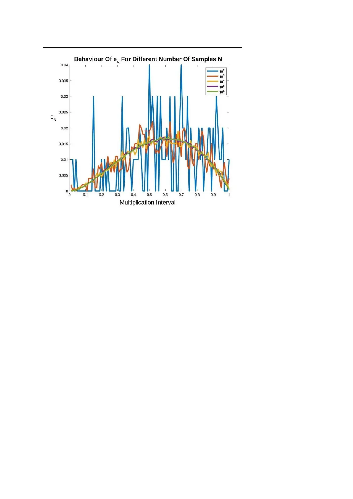
manuscript No. (will be inserted by the editor) How T o Catch A Lion In The Desert - On The Solution Of The Cov erage Directed Generation (CDG) Pr oblem Ravi v Gal · Eldad Haber · Brian Irwin* · Bilal Saleh · A vi Ziv Receiv ed: date / Accepted: date Abstract The testing and verification of a complex hardware or software system, such as modern integrated circuits (ICs) found in ev erything from smartphones to servers, can be a dif ficult process. One of the most dif ficult and time-consuming tasks a verification team faces is reaching coverage closure, or hitting all events in the cov erage space. Covera ge-dir ected-generation (CDG), or the automatic generation of tests that can hit hard-to-hit cov erage events, and thus provide cov erage closure, holds the potential to save verification teams significant simulation resources and time. In this paper , we propose a new approach to the CDG problem by formulating the CDG problem as a noisy deri vati ve free optimization (DFO) problem. Ho wev er , this formulation is complicated by the fact that deri vati ves of the objectiv e function are unav ailable, and the objective function ev aluations are corrupted by noise. W e solve this noisy optimization problem by utilizing techniques from direct optimiza- tion coupled with a rob ust noise estimator , and by le veraging techniques from in verse problems to estimate the gradient of the noisy objecti ve function. W e demonstrate the efficienc y and reliability of this ne w approach through numerical experiments with an abstract model of part of IBM’ s NorthStar processor , a superscalar in-order processor designed for servers. Keyw ords Hardware V erification · Co verage Directed Generation · Deri vati ve Free Optimization · Statistical Parameter Estimation · In verse Problems * Corresponding author . Ravi v Gal · Bilal Saleh · A vi Ziv IBM Research Laboratory in Haifa, Haifa, Israel E-mail: { RA VIVG, BILAL, AZIV } @il.ibm.com Eldad Haber · Brian Irwin Department of Earth and Ocean Science, The Univ ersity of British Columbia, V ancouver , BC, Canada E-mail: { haber , birwin } @eoas.ubc.ca 2 Ravi v Gal et al. 1 Introduction V erification of a complex hardware or software system, such as modern inte grated cir cuits (ICs), can be a challenge. In principle, one would like to test every state or ev ent that the system can reach, and observe that the system functions as intended. Howe ver , for comple x systems, this is impossible, as the number of possible states is so large that it is impractical to test each state indi vidually . T o this end, it is common to define a large, but finite, random set of tests or test instances , also referred to as test stimuli , that are drawn from the distribution of all possible tests, and apply them to the design-under-test (DUT) to be tested. This paper targets verification environments that utilize biased random stimuli generator s to generate test stimuli. The stimuli generator uses, as its input, test tem- plates that bias the generation to ward targeted areas and features of the verified de- sign. A test template comprises a set of parameters, or directives, where each param- eter is a set of weight-value pairs. W e refer to the output stimuli of the random stimuli generator as a test instance. Even with a smart choice of test stimuli, one may hav e great difficulty hitting a number of key events to be tested. These ev ents are often referred to as har d-to- hit ev ents. This is because the mapping from test parameters to events is unknown, and can be highly nontri vial. Therefore, one of the most difficult and time-consuming tasks a v erification team faces is reaching cov erage closure, or , in other words, hitting all cov erage events, including hard-to-hit ev ents. Understanding why certain ev ents are difficult to hit, and how the y can be hit, requires both verification expertise and a deep understanding of the design under test. Moreover , generating test instances that hit such ev ents is often an iterati ve trial and error process that consumes significant simulation resources and verification team time. Therefore, it is desirable to have an automatic solution for improving the probability of hitting hard-to-hit e vents. Covera ge-dir ected-generation (CDG), or the automatic generation of test instances, is a concept that has long been on the wish list of verification teams, and the tar get of a vast amount of research. Many techniques have been proposed to tackle the CDG problem, ranging from formal methods, via AI algorithms, to data analytics and ma- chine learning techniques (see [ 10 ], [ 12 ], [ 5 ] and references within). These techniques did not mature to be widely used in industry for v arious reasons, including the scala- bility of the solution, dif ficulty in applying it, and the quality of the proposed solution. As a result, reaching cov erage closure remains almost entirely a manual process. The goal of this work is to propose a new approach for the solution of the CDG problem and increasing the probability of hitting hard-to-hit events. Finding how to hit a low probability event in a large space is sometimes humourously referred to as finding “how to catch a lion in the desert”, originated by the seminal paper of P ´ etard [ 14 ]. W e propose a method that solves the problem by minimizing a cost function that increases the probability of hitting the hard-to-hit event(s). W e show that such an approach can lead to an efficient solution of the problem, especially if it is coupled with a robust and ef ficient optimization algorithm. The rest of the paper is or ganized as follows. In Section 2 , we gi ve a mathematical background to the proposed approach. In Section 3 , we discuss solution techniques for the problem. These techniques are based on direct optimization methods coupled How T o Catch A Lion In The Desert - On The Solution Of The CDG Problem 3 with a robust noise estimator . In Section 4 , we describe the main experimental en vi- ronment used to test the proposed approach. In Section 5 , we perform a number of experiments that demonstrate the ef ficiency of our approach, and we summarize the paper in Section 6 . 2 Mathematical Background Let us mathematically formalize the testing process. Let θ ( t ) denote a random v ari- able, referred to as a test instance of test template t , and representing a test to be run by the DUT . Using directives , the test template t can be represented as a vector t = [ d 1 , . . . , d n ] composed of n directive weight vectors d j , j = 1 , . . . , n . Each directiv e d j is parametrized by a weight vector d j , where the weight vector is normalized to present a probability distribution. The space of all possible test templates is denoted by T , and is also known as the test templates skeleton . It is important to note that, while each test instance θ ( t ) is random, the directives and the test templates are not . The directi ves and test templates are deterministic parameters that define the random space and control the distribution of the test instances. In the testing and verification process, the main goal is to hit ev ery ev ent in the covera ge space C = { c 1 , ..., c m } , or space of all ev ents. Gi ven a test instance θ ( t ) , chosen from a probability space defined by the vector t ∈ T , one runs a simulation to obtain a random vector , s ( θ ) = [ s 1 , . . . , s m ] , s j ∈ { 0 , 1 } ∀ j , that is defined as a hit covera ge vector . The entries of the hit cov erage vector s are binary . If a particular ev ent in the cov erage space was hit by the specific test instance θ , the entry of the corresponding index in s is 1, and it is 0 otherwise. Clearly , since the test instances are generated randomly in a manner dependent on the parameters of the test template t , the vector s is also random and depends on t . T o this end, let e ( t ) = E  s ( θ ( t ))  (1) be the expected v alue of the hit coverage v ector s , and let e N ( t ) = 1 N ∑ j s j (2) be the empirical expectation of the hit cov erage vector estimated using N test in- stances generated from test template t . Note that while s j ∈ { 0 , 1 } ∀ j , the vector e = [ e 1 , . . . , e m ] and its empirical v alues are r eal . The j -th value in e ( t ) , e j , represents the probability of hitting the event c j using a test instance θ generated according to the distrib ution defined by t . T o compute the empirical expectation e N ( t ) of a hit cov- erage v ector, giv en a test template t , we can run N simulations, obtain s j , j = 1 , . . . , N hit coverage vectors, and average them. Clearly , such a process is computationally expensi ve, especially if we are to estimate e ( t ) accurately . T o demonstrate the above definitions, let us consider the following simple, b ut concrete example. 4 Ravi v Gal et al. Example 1: T esting The Multiplication of T wo Numbers Assume that we build a calculator that can compute the product of two numbers in the interval [ 0 , 1 ] . In a test instance, we need to randomly pick two numbers within the interval and compute their product. In this case, we hav e two directiv e weight vectors, d 1 and d 2 , that define how we choose each of the two numbers. For simplicity , in this case we assume that d 1 = d 2 = d , and therefore the test template t is just the single directive weight vector t = d . Next, we choose the parametrization of the test template, which defines the numbers in the interval [ 0 , 1 ] . For simplicity , we assume that t = [ t 1 , . . . , t k ] are the probabilities of choosing a number in the interval [ 0 , 1 / k ] , . . . , ( 1 − 1 / k , 1 ] . Recall the space C is the space of all events, or coverage space. Let us define m = k different ev ents that correspond to the k cases that the output of the multiplication falls into one of the intervals [ 0 , 1 / k ] , . . . , ( 1 − 1 / k , 1 ] . Now , consider choosing the probability density parameterized by t . One tempting choice is to simply use the uniform distribution, setting t i = 1 / k , i = 1 , . . . , k . Clearly , this choice leads to less than optimal sampling of the cov erage space. For this case, it is easy see that e 1  e k If we further refine the intervals in the T and C spaces by letting k → ∞ , then the likelihood of hitting an ev ent that is at the right edge (close to 1) will approach 0, and therefore using a uniform distribution may not lead to a complete sampling of the cov- erage space, and we may end up with some unhit ev ents. Understanding this problem allows one to choose a sampling routine that gives a higher probability to numbers that are close to 1, and improv e the probability of sampling the whole co verage space. The above multiplication example can be clearly analyzed to obtain an optimal sampling scheme. Howe ver , in practice, this is very frequently not the case. The sys- tem under test may be highly nonlinear . In this case, one typically performs some probing of the space by randomly testing a number of sampling schemes, and then tries to improve the cov erage and sample as intelligently as possible. Howe ver , as previously discussed, hitting a hard-to-hit event may be difficult and require manual and labor intensiv e processes. Our goal is to improv e over such processes by auto- matically increasing the probability of hitting hard-to-hit ev ents. Obtaining e N ( t ) from t is an unkno wn function that is dictated by the simulator , and can be written as e N ( t ) = e ( t ) + ω ( t ) (3) Here, ω ( t ) is a noise vector that depends on the parameters, t . This noise vector ω gets a different value e very time we compute e N , giving us a noisy realization of the expected v alue of the hit coverage v ector . Let us define the tar get e vent(s), e tar ( t ) = P > e ( t ) . Depending on the specific prob- lem, e tar can be a vector or a number . For example, if we only want to hit the j -th ev ent, we can define P > as the j -th ro w of the identity matrix. In some cases, we aim to increase the probability of hitting a group of hard-to-hit e vents, and in this case P > corresponds to a few rows of the identity matrix. Maximizing the probability of How T o Catch A Lion In The Desert - On The Solution Of The CDG Problem 5 hitting the ev ents in e tar can now be formulated as the simple optimization problem max t  φ ( t ) = 1 > e tar ( t ) = E  1 > P > s ( θ ( t ))   (4) where 1 is a vector of all ones. There are a number of problems when attempting to solv e the maximization prob- lem defined by equation 4 . First, we do not hav e access to the objectiv e function directly . The objective function can only be ev aluated up to some unknown noise. Second, this noise is not necessarily stationary . That is, every time the objecti ve func- tion is called, a different noise v ector is generated, and, on top of that, the noise le vel can be different for different values of t . Third, for a fixed t , the noise corrupting the measurement of e ( t ) is likely different for each entry . In other words, the noise lev el is likely different for each ev ent e j . Fourth, a critical difference between this problem and the common problem of minimization under the expectation is that for the canonical stochastic programming problem, the random variable is dra wn from a fixed distribution. Here, the distribution is parameterized by t , and therefore, as we change the v alues of the parameters we optimize, we obtain a different distribution with a possibly different noise signature. T o illustrate the abov e, we continue with our discussion of Example 1. Example 1: T esting The Multiplication of T wo Numbers - Continued W e choose k = 100 segments, and choose the entries of t to grow quadratically in the interval [ 0 , 1 ] , and normalize such that they sum to 1. This implies that we hav e a higher probability of choosing larger numbers compared with smaller numbers. Giv en this test template, we compute the empirical hit cov erage vector , e N ( t ) , for N = 10 i , i = { 2 , 3 , 4 , 5 , 6 } . The results are plotted in Figure 1 . The results demonstrate how noisy the function can be when the number of realizations is small, and ho w the probability con verges as the number of samples grows. Also note how low the probability of choosing numbers close to 1 is, ev en when t is chosen to grow quadratically . T o find a t that further improv es the probability of hitting the rightmost element in the empirical hit coverage vector e N , by setting 1 > P > = [ 0 , . . . , 0 , 1 ] , one can compute an objectiv e function that maximizes the probability of hitting the rightmost element. 3 Solution T echniques The main problem under consideration here, the CDG problem, can be formulated as a deriv ative free optimization (DFO) problem where the objectiv e function un- der consideration is noisy . The topic has been considered by many authors, such as C.T . Kelle y , J. Nocedal, and K. Scheinberg, using dif ferent techniques, ranging from stochastic methods [ 4 ], direct search methods [ 9 ], and gradient based methods [ 1 ]. In this paper , we experiment with three optimization techniques: an implicit filter- ing based technique, a steepest descent based technique, and a Broyden-Fletcher- Goldfarb-Shanno (BFGS) based technique. While we have directly used an implicit filtering technique, we have modified existing steepest descent and BFGS techniques 6 Ravi v Gal et al. Fig. 1 Evaluation of e N for the values N = 10 i , i = { 2 , 3 , 4 , 5 , 6 } on the simple two number multiplication model problem. W e choose k = 100 segments, and choose the elements of t to gro w quadratically in the interval [ 0 , 1 ] , and normalize such that the y sum to 1. Note ho w noisy the function can be when the number of realizations is small, and how the probability conv erges as the number of samples grows. Also note the low probability of hitting e vents at either end (close to 0 or 1) of the multiplication interval. from non-noisy unconstrained optimization in order to better deal with the noise in the problem. Below , we describe the algorithmic framew ork we used to solve the problem. 3.1 Optimization Problem Setup Giv en an objectiv e function f ( t ) , we re write it as f ( t ) = φ ( t ) + ω ( t ) (5) W e assume that φ ( t ) is a smooth function, and that ω ( t ) is noise. The noise ω is assumed to be uncorrelated with zero mean, and some unknown standard deviation σ . W e assume that the standard deviation σ ( t ) changes slowly with respect to t . For the CDG problem, we are unable to obtain the deriv atives of φ with respect to t , and therefore we turn to DFO methods. While there are man y DFO meth- ods, we turn our attention to local methods that are based on the numerical esti- mation of the gradient. Such methods have been studied extensiv ely in the last 30 How T o Catch A Lion In The Desert - On The Solution Of The CDG Problem 7 years [ 18 ], yielding successful software packages such as MCS, TOMLAB/LGO, and NEWUO A [ 8 , 15 , 17 ] (also see references within). Howe ver , when experimenting with the problem, we found that standard ap- proaches based on gradient estimation methods fail or work poorly when the noise lev el is high. T o explain this problematic observation, we first revie w the standard approach to such problems. A typical algorithm for such problems is composed of the following steps. 1. Evaluate the function f , its gradient ∇ f , and its approximate Hessian B . 2. Compute a descent direction z . 3. Update the solution using some relaxed line search or trust region method. Function and gradient ev aluations are typically done using finite differences. Let us revie w the process at some depth. Assume that we would like to compute the di- rectional deriv ative of f ( t ) in the direction v . It is common to use a central finite difference approach computing v > ∇ f ( t ) ≈ f ( t + h v ) − f ( t − h v ) 2 h (6) which giv es v > ∇ f ( t ) ≈ v > ∇ φ ( t ) + ¯ ω 2 h + h 2 N ( φ ( t ) , v ) (7) where ¯ ω is a random v ariable generated by combining the zero mean errors in the function ev aluations. It is evident that the approximation for v > ∇ f ( t ) is polluted with two types of errors. The first type of error, corresponding to the second term in equation 7 , is the error due to the noisy estimation of the function, and the second type of error, corresponding to the third term in equation 7 , is an error due to the nonlinearity of φ ( t ) . Unfortunately , these error terms hav e contradicting behaviours. While the second term in equation 7 requires as large an h as possible to reduce the error , the third requires a small h to obtain the same goal. In some cases, when the noise is small, and it is possible to obtain an estimate of the magnitude of the nonlinear residual, one can balance these terms, choosing h =  σ 2 ¯ N  1 3 where ¯ N is an estimate of the nonlinear residual. This approximation can be used in order to obtain a reasonable estimate of the gradient. Howev er , ev en with this choice of approximation, the estimate of the gradient may not be sufficiently accurate. Furthermore, estimating the noise and the nonlinear errors can be computationally difficult, and require additional function ev aluations using different sized stencils. Such work was proposed in [ 11 ]. Howe ver , ev en with an optimal stencil size, the noise can still be significant (see, for e xample, Figure 1 ). Indeed, e ven for the optimal h (assuming that both ¯ N and σ are known), the error corrupting v > ∇ f ( t ) scales as σ 2 3 , which only marginally improves the problem presented by the noise for large values of σ . 8 Ravi v Gal et al. In this w ork, we introduce a dif ferent approach to the optimization problem. Rather than estimating the noise by further function ev aluations, we view the prob- lem as a statistical in verse problem, where the solution has to be e valuated from noisy data. In the next subsection, we show how to use standard techniques from inv erse problems to estimate the behaviour of the objecti ve function f , and its gradient ∇ f . 3.2 Function And Gradient Approximation As Statistical Parameter Estimation Let us provide a dif ferent interpretation of the process of ev aluating the gradient of a noisy function. Let us consider a general linear model of the form f ( t + h v i ) = ¯ φ ( t ) + h v > i g + ω i (8) with k v i k = 1 and ω i being noise. Here, g is an unkno wn vector that is to be computed from the values of the objective function in points around t . Note that this linear approximation is not necessarily the T aylor expansion. It can be any linear model that approximates the function for a gi ven step size h and direction v i . Clearly , for smooth functions, as h → 0, the approximation con ver ges to the T aylor expansion. Now , assume that we hav e n directions, v 1 , . . . , v n . Using these directions, we obtain the following set of equations    f 1 . . . f n    =   1 h v > 1 1 . . . 1 h v > n    ¯ φ g  +    ω 1 . . . ω n    (9) which we rewrite as the simple linear system f = V b g + ω . (10) where b g = [ ¯ φ , g > ] > . Estimating b g from the noisy data f is a corner stone of statis- tical in verse problems [ 19 ]. It is therefore straight forward to use inv erse problems techniques for the estimation of the av erage function value, ¯ φ , and gradient g . W e further assume that we hav e some prior estimate of b g , b g 0 . If no such estimate is a vailable, then we can choose b g 0 = 0 . Such an estimate can be obtained if we kno w something about the function f , or if we computed b g at a nearby point. For example, if b g was computed during a previous iteration, we can use this value from the previous iteration as b g 0 . A new estimate of b g can be obtained by solving the following ridge regression type minimization problem min b g  1 2 k V b g − f k 2 + α 2 k b g − b g 0 k 2  (11) Giv en the regularization parameter , α , the problem has the closed form solution b g α = ( V > V + α I ) − 1 ( V > f + α b g 0 ) (12) The regularization parameter α is chosen based on the noise lev el. When the noise lev el is unkno wn, as in our problem, the Generalized Cross V alidation (GCV) method How T o Catch A Lion In The Desert - On The Solution Of The CDG Problem 9 can be used to choose α , and obtain an unbiased estimate of the noise lev el [ 6 ]. This is done by minimizing the GCV function for this problem GCV ( α ) = k ( I − A ( α ))( f − V b g 0 ) k 2 trace ( I − A ( α )) 2 (13) where A ( α ) = V ( V > V + α I ) − 1 V > . Minimizing the GCV function in equation 13 in 1D can be done using a bisection method [ 3 ]. As we will later see in the numerical experiments section, the values obtained using the abov e approach can provide a significant advantage compared to the simple finite difference approximations employed in classical noisy optimization approaches. 3.3 Solution Algorithm Below , we present our solution algorithm in pseudocode. Algorithm 1 outlines the gradient based steepest descent technique and the BFGS approximation. As a comparison to our approach, we use implicit filtering as presented in [ 9 ]. The implicit filtering algorithm does not require any gradient approximations, and only relies on the noisy values of f itself. Our algorithm adapts standard descent methods for non-noisy problems by using the GCV estimated ¯ φ and g in place of the values of f and ∇ f at each point, and performs a simple line search procedure. A few comments are in order – Minimizing the GCV function is not, in general, a computationally cheap process. Howe ver , for the problem at hand, function ev aluation is very expensi ve and the number of v ariables does not exceed the few thousands. In this case, in vesting some work to obtain the best direction possible is justified. – For problems where function ev aluation is cheap, one may not find our approach attractiv e. – Efficient ways to minimize the GCV function that use stochastic trace estimators can make the process of solving the problem relativ ely fast. Here we have used the technique proposed in [ 7 ] to obtain the solution of the problem using Krylov space decomposition. Before presenting the results from numerical experiments using our approach, we first describe the system used for the numerical experiments: an abstract model of part of IBM’ s NorthStar processor . 4 The NorthStar Pipeline As a lightweight experimental environment, we employ a high-level software model of the two arithmetic pipes of the NorthStar superscalar in-order processor and the 10 Ravi v Gal et al. Algorithm 1 Gradient Based Steepest Descent T echnique procedur e D E SC E N T T E C H NI Q U E % Initialize minimization algorithm it er ← 0 % Iteration count µ l s ← 10 % Initialize line search parameter l s break ← False % Line search break flag t ← t init t o pt ← t init ¯ φ o pt ← ∞ Evaluate f ( t + h v ) in n random directions v Estimate ¯ φ and g by solving 12 using GCV Approximate the in verse Hessian, B (in the case of BFGS) or set B = I while T rue do it er ← it er + 1 t ol d ← t ¯ φ ol d ← ¯ φ g ol d ← g l sIt er ← 1 % Line search iteration count while T rue do t ← t ol d − µ l s Bg ol d Evaluate f ( t + h v ) in n directions v Estimate ¯ φ , g , and average noise le vel || ω || if ¯ φ < ¯ φ ol d + 2 || ω || then if ¯ φ < ¯ φ o pt then t o pt ← t ¯ φ o pt ← ¯ φ break µ l s ← µ l s / 2 % Shrink line search parameter l sIt er ← l sIt er + 1 if l sIt er > Max. # line search iterations then l s break ← T rue % Line search break break if l sIt er = 1 then µ l s ← 2 µ l s % Expand line search parameter % Check algorithm termination conditions if l s break = T rue then break if it er > Max. # iterations then break dispatch unit, also used in [ 5 ]. The NorthStar processor , also kno wn as the RS64-II or PowerPC A50, was released by IBM in the late 1990s, featuring a RISC instruction set architecture [ 2 ]. The high-le vel software model consists of two main components. First, a biased random stimuli generator that generates programs, and second, a soft- ware simulator of the NorthStar processor’ s dispatch unit and two arithmetic pipes that ex ecutes the randomly generated programs. The NorthStar has two pipes, one simple and one complex (see Figure 2 ). Each of the pipes comprises three stages: data fetch, execution, and write-back. One of the pipes, the simple pipe, handles only simple instructions, such as ad d . The other pipe, the complex pipe, handles complex instructions, such as mul . The complex pipe can also handle simple instructions when the simple pipe is busy . The model supports fiv e types of instructions: simple instructions S im , three types of complex How T o Catch A Lion In The Desert - On The Solution Of The CDG Problem 11 Fig. 2 Schematic of the simulated NorthStar pipeline. There are two pipes of 3 stages, one simple pipe S and one comple x pipe C . In addition, L/S represents the processor’ s load store unit, and BR the branch prediction unit. instructions Cm 1 , C m 2 , C m 3 that dif fer in the time they spend in the execution stage (1, 2, and 3 cycles respectiv ely), and N o p , which represents all instructions that are not ex ecuted in the arithmetic pipes. The actual ex ecution time can be longer due to data dependencies between instructions. T o maintain simplicity , we assume the processor has only eight registers and instructions use one source and one target register . In addition, the processor has a condition register C R , which some instructions read from and write to. In each cycle, up to two instructions are fetched, according to the instruction’ s type and the state of the pipes. T est templates t for the NorthStar software model are defined by four direc- tiv e weight vectors t = [ d 1 , d 2 , d 3 , d 4 ] , and control the distribution that the biased random stimuli generator component generates random programs from. Each direc- tiv e weight vector defines a probability distribution. The first directiv e weight vector d 1 = IW = [ W N o p , W Sim , W Cm 1 , W Cm 2 , W Cm 3 ] contains instruction set selection weights, and controls the mnemonic of the generated instructions. The second and third di- rectiv es af fect the behaviour of the source and target registers. The second directiv e weight vector d 2 = SW = [ W S 0 , ..., W S 7 ] contains source re gister weights, and the third directiv e weight v ector d 3 = T W = [ W T 0 , ..., W T 7 ] contains target register weights. The fourth directiv e weight vector d 4 = CW = [ W C 0 , W C 1 ] controls the conditional re gister . Thus, one can express a test template as the 23 entry v ector t = [ IW , S W , T W , CW ] . The cov erage space C is a cross-product [ 16 ] of the instructions in stage 0 of the complex and simple pipes (5 and 2 possible values respectiv ely), two indicators for whether stage 1 of each pipe is occupied, and an indicator for whether the instruction in S 1 is using the conditional re gister . An e vent is defined by assigning values to each coordinate. F or example, the e vent ( C 2 , S im , 0 , 0 , 0 ) means that C 2 and Sim are hosted 12 Ravi v Gal et al. at stage 0 of the complex and simple pipes, stage 1 of both pipes is not occupied, and the conditional re gister is not used. Clearly , the size of the coverage space size is | C 0 I nst × S 0 I nst × C 1 U sed × S 1 U sed × S 1 CR | = | 5 × 2 × 2 × 2 × 2 | = 80. Howe ver , out of this space, only 54 events are legal. For example, the 8 ev ents spanned by the subspace ( Sim , N o p , ∗ , ∗ , ∗ ) , where * indicates a wildcard that can be any value, are illegal because if S 0 is free, then the simple instruction should ha ve been fetched into the simple pipe. During simulation, cov erage is tracked for a time interval of 100 cycles, starting at c ycle 10. An ev ent is considered hit by the test instance if it was hit at least once during this time interval. 5 Numerical Experiments In this section, we compare the performance of the implicit filtering, steepest descent, and BFGS techniques numerically using the NorthStar pipeline simulator described abov e in section 4 . 5.1 Initial Exploration As an initial exploration of e ( t ) for the NorthStar, we first ran 5000 random test templates drawn from T according to the Dirichlet distribution Dir ( 1 ) . Using these 5000 test templates, we hit all events in the coverage space C at least once. W e also found the hardest ev ent to hit to be e vent c hard = ( C 2 , N o p , 0 , 1 , 0 ) . The single best test template hit e vent c hard with probability p ( c hard ) = 0 . 15. Based on applied domain knowledge, it was deduced that the test template defined by IW = ( 0 . 5 , 0 . 2 , 0 , 0 . 3 , 0 ) , S W = T W = ( 1 , 0 , 0 , 0 , 0 , 0 , 0 , 0 ) , and C R = ( 1 , 0 ) would yield the best chance of hitting ev ent c hard 1 . This test template t = [ 0 . 5 , 0 . 2 , 0 , 0 . 3 , 0 , 1 , 0 , 0 , 0 , 0 , 0 , 0 , 0 , 1 , 0 , 0 , 0 , 0 , 0 , 0 , 0 , 1 , 0 ] will giv e high weights to N o p , S im , and C m 2 , will create dependencies between the source and target registers, and will not use the condition register C R . Experimen- tally , by averaging over 100000 runs of the simulator , this template was observed to yield a hit probability of p ( c hard ) = 0 . 4. Below , we continue to use values averaged ov er 100000 runs of the simulator to define a high quality estimate, or “true” value of p ( c hard ) . Howe ver , as we show below , both the implicit filtering and steepest de- scent based techniques are able to automatically discov er test templates that achiev e p ( c hard ) = 0 . 4 or close to 0 . 4 with a modest budget of total runs of the NorthStar simulator . 5.2 Event c hard Objectiv e Function As w as the case when analyzing ho w to maximize the probability of hitting the right- most element in the empirical hit coverage vector for the two number multiplica- 1 There are many other templates with different v alues of S W and T W that achie ve the same probability . How T o Catch A Lion In The Desert - On The Solution Of The CDG Problem 13 Fig. 3 The landscape of the objectiv e function for maximizing the probability of hitting event c hard com- puted over two random directions y 1 and y 2 . Note the many local maxima, and the objective function’ s overall non-con vexity . Also, note the confusing ef fects of noise, such as overestimating probabilities when N is small. tion simulator in Section 2 , we can again choose P > to be a single ro w of the iden- tity matrix. Specifically , P > is now the row of the identity matrix corresponding to c hard . T o av oid explicity enforcing the constraint that the directiv e weight vectors IW , S W , T W , C W define properly normalized probability distributions, and thus solv- ing a constrained optimization problem, we instead pass the values obtained from the optimization algorithms through the standard softmax function to ensure valid prob- ability distributions before passing them to the program generator component of the NorthStar software model. In Figure 3 , we plot the objectiv e function for maximizing p ( c hard ) sliced over two random directions y 1 and y 2 , for N = 10 and N = 1000 simulator runs per point respectiv ely . The uniform test template t uni , defined by IW = ( 0 . 2 , 0 . 2 , 0 . 2 , 0 . 2 , 0 . 2 ) S W = T W = ( 0 . 125 , 0 . 125 , 0 . 125 , 0 . 125 , 0 . 125 , 0 . 125 , 0 . 125 , 0 . 125 ) C W = ( 0 . 5 , 0 . 5 ) defines the origin in Figure 3 , and is the starting point for all the optimization ex- periments in the follo wing subsections. Once again, e valuating the objectiv e function first consists of passing a vector in R 23 through standard softmax functions ov er the 1 st to 5 t h , 6 t h to 13 t h , 14 t h to 21 st , and 22 nd to 23 rd components. After using the stan- dard softmax function to ensure the 4 directive weight v ectors define valid probability distributions, we pass the template defined by these 4 directive weight vectors to the biased random stimuli generator , and track the coverage of the generated random pro- grams over 100 cycles. Note the many local minima, the objective function’ s overall non-con vexity , and how increasing the number of simulator runs per point does not substantially alleviate the non-con vexity . 5.3 Implicit Filtering T echnique W e use implicit filtering to maximize p ( c hard ) , which is equiv alent to minimizing − p ( c hard ) . T able 1 shows the results of a typical successful run of the implicit filter- ing algorithm. N denotes the number of simulator runs we use to estimate e N ( t ) at 14 Ravi v Gal et al. Fig. 4 V isualizing the ev olution of the hit probability estimators from T able 1 during the successful im- plicit filtering run. p ( c hard ) denotes the reference “true” value, which is calculated by averaging ov er 100000 runs of the simulator at a gi ven template t . The x-axis I is the iteration number . Note how f ∗ consistently ov erestimates the probability , whereas ¯ φ generally understimates the probability , but then con verges to the “true” v alue as the algorithm progresses. each template, and n is the number of random directions v . The algorithm was set to terminate after 50 iterations, or the stencil size h decreased belo w 1e-3. Ov erall, with a modest budget of 15000 total simulations 2 , we are able to automatically get within 0 . 01 of the best hit probability of p ( c hard ) = 0 . 4. Additionally , we also present the value of ¯ φ estimated by fitting the regularized linear model defined by equation 11 at each iteration. Figure 4 compares the behaviour of f ∗ , ¯ φ , and the “true” value of p ( c hard ) av eraged ov er 100000 simulator runs. It is worth noting that the fitted ¯ φ value appears to be a better estimator of p ( c hard ) than the values of f ∗ , which is not unexpected giv en it incorporates information from more runs of the simulator, and nearby points. T able 1 only shows a typical successful run of implicit filtering. The algorithm can also unsuccessfully terminate yielding templates achieving p o pt ( c hard ) = 0. As a result, we experiment with the expected performance of the algorithm for different parameter values in T able 2 . W e also in vestigate the tradeoff between the number of samples N used to estimate e N ( t ) at each template, and the number of random directions n , at each iteration. For each set of N and n values, we ensemble results ov er 25 independent runs, and, as in T able 1 , h init = 50, and the algorithm was set to terminate after 50 iterations, or the stencil size decreased below 1e-3. Overall, we see that the implicit filtering technique is not always very reliable. This is exemplified by the “Failures” column in T able 2 , which shows that e ven for relativ ely large per iteration budgets, the algorithm can still fail to ever hit the ev ent c hard . Specifically , a failure is defined as the algorithm terminating at a test template 2 (24 Iterations) × ( 25 Points Iteration ) × ( 25 Simulations Point ) = 15000 Simulations How T o Catch A Lion In The Desert - On The Solution Of The CDG Problem 15 Implicit Filtering History ( N = 25, n = 25, h init = 50) I f ∗ ¯ φ Update t o pt ? h p ( c hard ) 1 0 0 T rue 50 0.016 2 0 0 False 50 0 3 0.160 7.15e-5 T rue 25 0 4 0.080 8.62e-5 False 25 0.099 5 0.160 0.043 False 12.5 0.099 6 0.320 0.032 T rue 6.25 0.101 7 0.400 0.063 T rue 6.25 0.142 8 0.280 0.066 False 6.25 0.339 9 0.440 0.245 T rue 3.125 0.343 10 0.520 0.227 T rue 3.125 0.325 11 0.600 0.814 T rue 3.125 0.341 12 0.440 0.264 False 3.125 0.383 13 0.520 0.297 False 1.5625 0.385 14 0.560 0.270 False 7.8125e-1 0.382 15 0.640 0.350 T rue 3.90625e-1 0.388 16 0.520 0.390 False 3.90625e-1 0.363 17 0.560 0.346 False 1.953125e-1 0.364 18 0.480 0.346 False 9.765625e-2 0.363 19 0.520 0.346 False 4.8828125e-2 0.360 20 0.560 0.370 False 2.44140625e-2 0.365 21 0.520 0.335 False 1.220703125e-2 0.365 22 0.560 0.353 False 6.103515625e-3 0.363 23 0.520 0.353 False 3.0517578125e-3 0.364 24 0.480 0.353 False 1.52587890625e-3 0.362 Summary of Final Results T otal # of Simulations = 15000 IW o pt = [ 0 . 5790 , 0 . 2010 , 0 , 0 . 2151 , 0 . 0049 ] S W o pt = [ 0 , 1 , 0 , 0 , 0 , 0 , 0 , 0 ] T W o pt = [ 1 , 0 , 0 , 0 , 0 , 0 , 0 , 0 ] CW o pt = [ 1 , 0 ] f o pt = 0 . 64, ¯ φ o pt = 0 . 35, p o pt ( c hard ) = 0 . 39 T able 1 Summary of a successful run of the implicit filtering algorithm. The algorithm is able to auto- matically get within 0 . 01 of the best c hard hit probability of 0 . 4 using a modest budget of 15000 total simulations. The optimization w as initialized at the uniform template t uni , and was set to terminate after 50 iterations were exceeded, or the stencil size shrank belo w 1e-3. I is the iteration number . 16 Ravi v Gal et al. Per Iteration Budget = 100 N n I s 2 [ I ] f o pt s 2 [ f o pt ] p o pt ( c hard ) s 2 [ p o pt ( c hard )] max { p o pt ( c hard ) } Failures 5 20 17.2 0.4 0.040 0.027 0.015 0.005 0.367 23 25 10 10 17.2 0.8 0.048 0.028 0.022 0.006 0.335 23 25 20 5 17.4 1.8 0.062 0.031 0.033 0.009 0.352 22 25 Per Iteration Budget = 625 N n I s 2 [ I ] f o pt s 2 [ f o pt ] p o pt ( c hard ) s 2 [ p o pt ( c hard )] max { p o pt ( c hard ) } Failures 5 125 18.3 3.8 0.344 0.225 0.104 0.022 0.365 16 25 25 25 18.5 5.7 0.192 0.083 0.104 0.025 0.377 17 25 125 5 17.3 2.0 0.017 0.007 0.014 0.005 0.337 24 25 Per Iteration Budget = 1250 N n I s 2 [ I ] f o pt s 2 [ f o pt ] p o pt ( c hard ) s 2 [ p o pt ( c hard )] max { p o pt ( c hard ) } Failures 5 250 18.1 2.7 0.320 0.227 0.105 0.025 0.375 17 25 10 125 19.4 5.1 0.444 0.164 0.183 0.029 0.396 11 25 25 50 19.5 10.4 0.259 0.106 0.143 0.032 0.394 15 25 50 25 17.6 2.8 0.066 0.033 0.041 0.013 0.388 22 25 125 10 17.7 4.5 0.058 0.026 0.044 0.015 0.394 22 25 250 5 17.4 3.2 0.014 0.005 0.012 0.004 0.299 24 25 Per Iteration Budget = 2500 N n I s 2 [ I ] f o pt s 2 [ f o pt ] p o pt ( c hard ) s 2 [ p o pt ( c hard )] max { p o pt ( c hard ) } Failures 5 500 18.5 2.0 0.600 0.250 0.207 0.031 0.395 10 25 10 250 20.0 5.3 0.576 0.166 0.230 0.027 0.390 8 25 25 100 20.5 11.4 0.379 0.119 0.201 0.034 0.390 11 25 50 50 18.9 10.0 0.154 0.064 0.101 0.027 0.376 18 25 100 25 18.5 9.8 0.102 0.043 0.073 0.022 0.386 20 25 250 10 17.6 3.9 0.036 0.016 0.031 0.011 0.390 23 25 500 5 17.4 2.3 0.035 0.014 0.029 0.010 0.375 23 25 Per Iteration Budget = 5000 N n I s 2 [ I ] f o pt s 2 [ f o pt ] p o pt ( c hard ) s 2 [ p o pt ( c hard )] max { p o pt ( c hard ) } Failures 5 1000 19.7 1.1 0.912 0.077 0.281 0.010 0.389 2 25 10 500 20.8 4.0 0.748 0.113 0.285 0.018 0.395 4 25 25 200 20.8 5.8 0.539 0.080 0.276 0.021 0.393 5 25 50 100 21.3 12.5 0.404 0.081 0.246 0.030 0.389 8 25 100 50 20.7 13.7 0.294 0.072 0.204 0.034 0.392 11 25 200 25 19.0 12.8 0.131 0.046 0.103 0.029 0.394 18 25 500 10 18.6 11.5 0.084 0.030 0.074 0.023 0.397 20 25 1000 5 18.1 7.0 0.048 0.017 0.043 0.014 0.392 21 25 T able 2 Results of the implicit filtering based optimization technique compared over fixed per iteration budgets. Statistics are calculated o ver 25 independent runs for each combination of n and N , where a bar represents the sample a verage, and s 2 [ · ] represents the sample v ariance. N is equiv alent to simulator runs, and n is the number of directions in which we choose ne w test templates t . I is the number of iterations to termination, which occurs when the stencil size parameter reaches less than h = 0 . 001. A f ailure occurs when the algorithm terminates at a template with a “true” probability p o pt ( c hard ) = 0. How T o Catch A Lion In The Desert - On The Solution Of The CDG Problem 17 that has a p o pt ( c hard ) = 0, or in other words, e ven after averaging over 100000 sim- ulations at that template, event c hard was never hit. As expected, T able 2 sho ws the chances of a failure happening are reduced when the per iteration budget is increased, and the number of random directions n is increased. As a general trend, trading off simulation runs N for random directions n , given a fixed per iteration budget, is ben- eficial for the performance of implicit filtering. Only for very small values of N , such as N = 5, does this trend appear to break down. As it is undesirable for ho w many different parameter choices the algorithm fails more than half the time. W e now in- vestigate if a gradient-based algorithm performs better o verall. 5.4 Steepest Descent T echnique Now , we use Algorithm 1 to maximize p ( c hard ) , which is again equi valent to mini- mizing − p ( c hard ) . T able 3 shows the results of a typical successful run of the steepest descent algorithm. The algorithm was set to terminate after 50 iterations, or the line search break flag was set after 10 consecutiv e line search failures. The line search parameter µ l s was initialized to 10. Overall, with a modest budget of 21875 total simulations 3 , we are able to automatically get within 0 . 09 of the best hit probability of p ( c hard ) = 0 . 4. Note that the term “total iterations” refers to all the iterations re- quiring computations, including the failed line searches. For e xample, iteration 12 in T able 3 contributed 4 total iterations, as iteration 12 required 4 line search iterations. Figure 5 compares the behaviour of ¯ φ , and the “true” v alue of p ( c hard ) . In general, ¯ φ tracks p ( c hard ) closely , b ut with a tendenc y to v ary more slo wly . This is because of the av eraging effect of the algorithm. Similar to T able 2 , T able 4 in vestigates the expected performance of Algorithm 1 for different parameter values. Like with T able 2 , for each set of N and n values, we ensemble over 25 independent runs, and, as in T able 3 , h = 5 and µ l s is initialized to 10, and the algorithm was set to terminate after 50 iterations, or the line search break flag was set after 10 consecuti ve line search failures. Overall, the gradient based steepest descent technique appears much more reli- able than the implicit filtering technique. Algorithm 1 almost always terminates at a template that at least hits the e vent c hard a minimum of once in 100000 simulation runs. It is also worth noting that in most cases ¯ φ underestimates p ( c hard ) , sometimes by a large margin of up to almost 0.2. The authors conjecture this may be due to a relativ ely large choice of h , which is not refined during Algorithm 1 . The effects of a relativ ely large h should be especially pronounced if the optima are rather sharp, which gi ven domain knowledge, is not unlikely for this problem. Howe ver , as with the implicit filtering technique, the steepest descent algorithm’ s performance strongly benefits from trading off N for n , giv en a fixed per iteration budget. For both algo- rithms, it appears that in general, coarsely sampling many points is preferable to sampling a few points with high accurac y at each point. 3 (35 T otal Iterations) × ( 25 Points Iteration ) × ( 25 Simulations Point ) = 21875 Simulations 18 Ravi v Gal et al. Steepest Descent History ( N = 25, n = 25, h = 5) I ¯ φ k g k k ω k µ l s Update t o pt ? p ( c hard ) 1.1 0.018 0.0358 1.24e-3 10 T rue 0.017 2.1 0.029 0.1149 1.75e-4 20 T rue 0.022 3.4 0.030 0.0483 2.22e-4 5 T rue 0.022 4.1 0.027 0.0336 3.37e-3 5 F alse 0.022 5.1 0.027 0.0336 7.73e-3 10 False 0.025 6.1 0.021 0.0231 5.10e-3 20 False 0.028 7.1 0.021 0.0218 7.31e-3 40 False 0.040 8.1 0.026 0.0249 8.59e-3 80 False 0.062 9.1 0.030 0.0221 1.01e-2 160 False 0.088 10.1 0.034 0.0452 3.49e-3 320 True 0.027 11.3 0.145 0.1747 4.68e-3 160 True 0.333 12.4 0.147 0.1313 3.49e-2 20 True 0.339 13.1 0.155 0.1118 1.70e-2 20 True 0.331 14.3 0.241 0.2345 2.20e-4 10 True 0.312 15.10 0.031 0.2225 5.89e-4 1.953125e-2 False 0.314 Summary of Final Results T otal # of Simulations = 21875 IW o pt = [ 0 . 4377 , 0 . 1642 , 0 . 2597 , 0 . 1368 , 0 . 0015 ] S W o pt = [ 0 , 0 , 0 , 0 , 1 , 0 , 0 , 0 ] T W o pt = [ 0 , 1 , 0 , 0 , 0 , 0 , 0 , 0 ] CW o pt = [ 1 , 0 ] ¯ φ o pt = 0 . 24, p o pt ( c hard ) = 0 . 31 T able 3 Summary of a successful run of the steepest descent algorithm (Algorithm 1 ). The algorithm is able to automatically get within 0 . 09 of the best c hard hit probability of 0 . 4 using a modest budget of 21875 total simulations. The optimization w as initialized at the uniform template t uni , and was set to terminate after 50 main iterations were exceeded, or after 10 consecutiv e line search failures. I is the iteration number , formatted so the number after the decimal point represents the final line search iteration for the gi ven main iteration. 5.5 BFGS T echnique Finally , following the frame work of Algorithm 1 , we use BFGS to minimize − p ( c hard ) . Specifically , we use a limited-memory implementation of the BFGS method, also re- ferred to as L-BFGS. T o compute the BFGS directions, we use the L-BFGS two-loop recursion detailed on page 225 of [ 13 ]. W e set the initial in verse Hessian approxima- tion to be a scaled version of the identity matrix, where the scaling factor is gi ven by equation 9.6 on page 226 of [ 13 ]. As a result, a back tracking line search starting with µ l s = 1 at each iteration, and refining by a factor of two for each line search failure, How T o Catch A Lion In The Desert - On The Solution Of The CDG Problem 19 Per Iteration Budget = 100 N n I t s 2 [ I t ] ¯ φ o pt s 2 [ ¯ φ o pt ] p o pt ( c hard ) s 2 [ p o pt ( c hard )] max { p o pt ( c hard ) } Failures 5 20 82.5 290.2 0.164 0.013 0.124 0.016 0.375 0 25 10 10 81.7 1.04e3 0.041 7.13e-4 0.077 0.010 0.372 3 25 20 5 93.8 168.6 0.020 2.41e-4 0.022 0.002 0.165 12 25 Per Iteration Budget = 625 N n I t s 2 [ I t ] ¯ φ o pt s 2 [ ¯ φ o pt ] p o pt ( c hard ) s 2 [ p o pt ( c hard )] max { p o pt ( c hard ) } Failures 5 125 79.6 2.1 0.180 7.27e-5 0.355 0.001 0.397 0 25 25 25 47.7 645.9 0.337 0.085 0.163 0.017 0.367 0 25 125 5 94 246.0 0.020 1.47e-4 0.018 0.001 0.159 11 25 Per Iteration Budget = 1250 N n I t s 2 [ I t ] ¯ φ o pt s 2 [ ¯ φ o pt ] p o pt ( c hard ) s 2 [ p o pt ( c hard )] max { p o pt ( c hard ) } Failures 5 250 79.7 2.0 0.183 3.48e-5 0.375 3.44e-4 0.399 0 25 10 125 80.3 2.3 0.182 4.00e-5 0.362 8.63e-4 0.400 0 25 25 50 80.5 3.0 0.181 2.07e-4 0.340 0.001 0.384 0 25 50 25 43.5 646.3 0.211 0.024 0.151 0.019 0.394 0 25 125 10 71.2 951.2 0.061 0.003 0.118 0.011 0.379 0 25 250 5 98.0 336.5 0.019 8.95e-5 0.036 0.004 0.218 10 25 Per Iteration Budget = 2500 N n I t s 2 [ I t ] ¯ φ o pt s 2 [ ¯ φ o pt ] p o pt ( c hard ) s 2 [ p o pt ( c hard )] max { p o pt ( c hard ) } Failures 5 500 80.2 1.8 0.185 1.40e-5 0.381 2.15e-4 0.402 0 25 10 250 79.6 1.8 0.185 2.18e-5 0.381 2.00e-4 0.400 0 25 25 100 79.2 2.5 0.184 3.33e-5 0.358 0.001 0.397 0 25 50 50 79.4 1.8 0.183 1.04e-4 0.338 0.002 0.398 0 25 100 25 44.2 585.1 0.250 0.043 0.189 0.017 0.382 0 25 250 10 80.0 1.76e3 0.054 0.002 0.120 0.012 0.344 0 25 500 5 101.5 99.0 0.019 8.10e-5 0.044 0.006 0.331 7 25 Per Iteration Budget = 5000 N n I t s 2 [ I t ] ¯ φ o pt s 2 [ ¯ φ o pt ] p o pt ( c hard ) s 2 [ p o pt ( c hard )] max { p o pt ( c hard ) } Failures 5 1000 80.6 1.6 0.185 1.01e-5 0.385 2.02e-4 0.400 0 25 10 500 80.1 3.3 0.185 1.16e-5 0.387 8.26e-5 0.402 0 25 25 200 80.0 2.4 0.186 2.28e-5 0.378 5.03e-4 0.402 0 25 50 100 80.0 2.1 0.182 4.65e-5 0.364 7.69e-4 0.399 0 25 100 50 79.9 1.6 0.185 1.43e-4 0.354 0.002 0.395 0 25 200 25 46.7 442.7 0.207 0.012 0.177 0.018 0.376 0 25 500 10 89.1 1.65e3 0.057 0.001 0.126 0.015 0.384 2 25 1000 5 99.9 326.2 0.027 4.83e-4 0.052 0.005 0.213 7 25 T able 4 Results of the steepest descent based optimization technique compared over fixed per iteration budgets. Statistics are calculated o ver 25 independent runs for each combination of n and N , where a bar represents the sample a verage, and s 2 [ · ] represents the sample v ariance. N is equiv alent to simulator runs, and n is the number of directions in which we choose new test templates t . I t is the number of total iterations to termination, which includes all line searches. T ermination occurs after 50 iterations, or 10 consecutive failed line searches. A failure occurs when the algorithm terminates at a template with a “true” probability p ( c hard ) = 0. 20 Ravi v Gal et al. Fig. 5 V isualizing the ev olution of the hit probability estimators from T able 3 during the successful run of the steepest descent algorithm (Algorithm 1 ). p ( c hard ) denotes the reference “true” value, which is calculated by av eraging over 100000 runs of the simulator at a giv en template t . The x-axis shows the iteration number , where the v alue after the decimal point is the final line search iteration number for the giv en main iteration. Note how ¯ φ understimates the “true” probability , especially to wards the end of the run. was employed. Howe ver , we set the memory value, m , for our L-BFGS implemen- tation to m = 100, which was almost always greater than the number of iterations before termination. As a result, almost all of the time our L-BFGS implementation was equi valent to a standard BFGS implementation. Of the three algorithms we tested, the L-BFGS implementation had the most dif- ficulty obtaining test templates achieving close to p ( c hard ) = 0 . 4, and is not compet- itiv e with either implicit filtering or steepest descent. As with T ables 2 and 4 , T able 5 in vestigates the expected performance of BFGS for different parameter values. Like with T able 4 , for each set of N and n values, we ensemble over 25 independent runs, h = 5, and the algorithm was set to terminate after 50 iterations, or the line search break flag was set after 10 consecuti ve line search failures. Whereas T ables 2 and 4 sho w that with a budget of 625 simulations per iteration, n = 25, and N = 25, the implicit filtering and steepest descent techniques on average achiev e p o pt ( c hard ) = 0 . 104 and p o pt ( c hard ) = 0 . 163 respectively , T able 5 shows the L-BFGS method only achiev es p o pt ( c hard ) = 0 . 018 on a verage. Howe ver , as with the previous two algorithms, there is still a noticeable benefit from trading off N for n , giv en a fixed per iteration b udget, and increasing the per iteration b udget can improv e performance. The L-BFGS technique also fails much less frequently than the implicit filtering technique. Overall though, the ensemble results suggest this method is infe- rior to the steepest descent based approach, and that the standard BFGS technique may need further modifications to handle the noise in this problem. How T o Catch A Lion In The Desert - On The Solution Of The CDG Problem 21 Per Iteration Budget = 100 N n I t s 2 [ I t ] ¯ φ o pt s 2 [ ¯ φ o pt ] p o pt ( c hard ) s 2 [ p o pt ( c hard )] max { p o pt ( c hard ) } Failures 5 20 32.7 423.9 0.032 4.27e-4 0.017 4.37e-7 0.019 0 25 10 10 45.8 497.4 0.023 1.51e-4 0.017 1.08e-4 0.061 1 25 20 5 33.2 682.2 0.012 8.69e-5 0.017 2.56e-6 0.024 0 25 Per Iteration Budget = 625 N n I t s 2 [ I t ] ¯ φ o pt s 2 [ ¯ φ o pt ] p o pt ( c hard ) s 2 [ p o pt ( c hard )] max { p o pt ( c hard ) } Failures 5 125 45.0 407.1 0.018 1.39e-4 0.022 4.13e-4 0.119 0 25 25 25 37.0 255.1 0.072 0.001 0.018 3.02e-5 0.044 0 25 125 5 57.5 187.3 0.016 5.15e-5 0.016 1.14e-4 0.059 2 25 Per Iteration Budget = 1250 N n I t s 2 [ I t ] ¯ φ o pt s 2 [ ¯ φ o pt ] p o pt ( c hard ) s 2 [ p o pt ( c hard )] max { p o pt ( c hard ) } Failures 5 250 51.5 232.4 0.019 1.46e-4 0.025 3.79e-4 0.112 0 25 10 125 51.0 244.1 0.030 0.002 0.048 0.005 0.270 0 25 25 50 49.0 215.7 0.028 9.34e-4 0.032 0.001 0.169 0 25 50 25 35.0 361.3 0.065 0.003 0.030 0.004 0.337 0 25 125 10 51.7 315.7 0.018 1.54e-4 0.018 1.36e-4 0.059 1 25 250 5 53.9 275.1 0.018 1.75e-4 0.016 1.34e-4 0.050 3 25 Per Iteration Budget = 2500 N n I t s 2 [ I t ] ¯ φ o pt s 2 [ ¯ φ o pt ] p o pt ( c hard ) s 2 [ p o pt ( c hard )] max { p o pt ( c hard ) } Failures 5 500 44.9 288.2 0.027 4.52e-4 0.041 0.002 0.203 0 25 10 250 46.5 282.4 0.026 3.87e-4 0.035 0.001 0.142 0 25 25 100 52 367.7 0.019 2.37e-4 0.026 7.01e-4 0.150 0 25 50 50 47.6 353.2 0.025 4.45e-4 0.031 8.01e-4 0.129 0 25 100 25 34.4 223.3 0.045 0.001 0.026 6.83e-4 0.144 0 25 250 10 51.2 423.3 0.018 3.91e-5 0.017 5.79e-5 0.045 1 25 500 5 58.5 135.6 0.014 5.50e-5 0.015 4.59e-5 0.026 2 25 Per Iteration Budget = 5000 N n I t s 2 [ I t ] ¯ φ o pt s 2 [ ¯ φ o pt ] p o pt ( c hard ) s 2 [ p o pt ( c hard )] max { p o pt ( c hard ) } Failures 5 1000 47.6 531.8 0.016 3.44e-6 0.022 1.98e-5 0.032 0 25 10 500 46.3 313.0 0.028 0.001 0.046 0.007 0.368 0 25 25 200 47.1 424.9 0.023 4.27e-4 0.033 0.001 0.161 0 25 50 100 47.4 391.3 0.016 2.28e-5 0.022 9.76e-5 0.065 0 25 100 50 47.8 452.7 0.017 8.17e-5 0.025 2.77e-4 0.094 0 25 200 25 31.2 215.4 0.062 0.013 0.018 1.35e-6 0.021 0 25 500 10 48.0 212.9 0.020 2.84e-4 0.021 1.86e-4 0.071 2 25 1000 5 58.6 345.5 0.015 2.56e-5 0.017 4.55e-5 0.037 1 25 T able 5 Results of the L-BFGS based optimization technique compared o ver fix ed per iteration budgets. Statistics are calculated over 25 independent runs for each combination of n and N , where a bar represents the sample average, and s 2 [ · ] represents the sample variance. N is equiv alent to simulator runs, and n is the number of directions in which we choose new test templates t . I t is the number of total iterations to termination, which includes all line searches. T ermination occurs after 50 iterations, or 10 consecutive failed line searches. A failure occurs when the algorithm terminates at a template with a “true” probability p ( c hard ) = 0. 22 Ravi v Gal et al. 6 Summary and Conclusions In this paper , we ha ve proposed three algorithms for solving the cov erage directed generation problem, all based on the key observation that the problem can be posed as deriv ativ e free optimization of a noisy objective function. By applying techniques from statistical parameter estimation and in verse problems, namely the generalized cross validation technique, we are able to generate quality estimates of the gradient of the noisy objectiv e function. W ith these gradient estimates, we are able to build algorithms that adapt the steepest descent and BFGS techniques from non-noisy con- tinuous optimization. The algorithm based on gradient descent, on av erage, empirically outperforms a simple, but sometimes surprisingly effecti ve, implicit filtering based approach. Nu- merical experiments with a high-level software model of part of IBM’ s NorthStar processor show that both the implicit filtering and steepest descent techniques are economical in terms of the total number of simulations required for them to be ef fec- tiv e, and how to best choose parameters giv en a fixed per iteration budget of simu- lations. Furthermore, all our algorithms are relatively easily parallelized in practice, as the repeated simulations at a single point N can be carried out in parallel, and this can further be done in parallel for the n points along the random directions, with the only major bottleneck being the work required during the decision to update the next template. W e suspect that the use of Inv erse Problem based techniques for gradient estima- tion can be further extended to the ev aluation of Hessians and in other contexts where the function and gradients are noisy , and this will be in vestigated in the future. Acknowledgements EH and BI’s work is supported by the Natural Sciences and Engineering Research Council of Canada (NSERC). RG, BS, and AZ’ s work is supported by IBM. Conflict of interest The authors declare that they ha ve no conflict of interest. References 1. Berahas, A.S., Byrd, R.H., Nocedal, J.: Deriv ativ e-free optimization of noisy functions via quasi- newton methods. SIAM Journal on Optimization 29 , 965–993 (2019) 2. Borkenhagen, J., Sorino, S.: 4th generation 64-bit powerpc-compatible commercial processor design (1999) 3. Burden, R.L., Faires, J.D.: Numerical Analysis. Cengage Learning (2010) 4. Conn, A., Scheinberg, K., V icente, L.: Introduction to Deri vati ve-Free Optimization. SIAM, Philadel- phia (2009) 5. Fine, S., Zi v , A.: Coverage directed test generation for functional v erification using bayesian netw orks. In: Design Automation Conference (2003) 6. Golub, G., Heath, M., W ahba, G.: Generalized cross-v alidation as a method for choosing a good ridge parameter . T echnometrics 21 , 215–223 (1979) 7. Golub, G.H., v on Matt, U.: Generalized cross-v alidation for large-scale problems. Journal of Compu- tational and Graphical Statistics 1 , 1–34 (1997) How T o Catch A Lion In The Desert - On The Solution Of The CDG Problem 23 8. Huyer, W ., Neumaier, A.: Global optimization by multilevel coordinate search. Journal of Global Optimization 14 , 331–355 (1999) 9. Kelley , C.: Implicit Filtering. SIAM, Philadelphia (2011) 10. Mishra, P ., Dutt, N.: Automatic functional test program generation for pipelined processors using model checking. In: Seventh Annual IEEE International W orkshop on High-Level Design V alidation and T est, pp. 99–103 (2002) 11. Mor ´ e, J.J., W ild, S.M.: Estimating computational noise. SIAM Journal on Scientific Computing 33 , 1292–1314 (2011) 12. Nativ , G., Mittermaier, S., Ur , S., Ziv , A.: Cost evaluation of cov erage directed test generation for the ibm mainframe. In: Proceedings of the 2001 International T est Conference, pp. 793–802 (2001) 13. Nocedal, J., Wright, S.: Numerical Optimization. Springer, Ne w Y ork (1999) 14. P ´ etard, H.: A contribution to the mathematical theory of big game hunting. American Mathematical Monthly (1938) 15. Pint ´ er , J.D.: Global Optimization in Action. Springer US (1996) 16. Piziali, A.: Functional V erification Coverage Measurement and Analysis. Springer (2004) 17. Powell, M.: The newuoa software for unconstrained optimization without deri vativ es. In: G.D. Pillo, M. Roma (eds.) Large-Scale Nonlinear Optimization, pp. 255–297. Springer , Boston, MA (2006) 18. Rios, L.M., Sahinidis, N.V .: Deri vativ e-free optimization: a review of algorithms and comparison of software implementations. Journal of Global Optimization 56 , 1247–1293 (2013) 19. T enorio, L.: An Introduction to Data Analysis and Uncertainty Quantification for In verse Problems. SIAM (2017)