Voltage stress minimization by optimal reactive power control

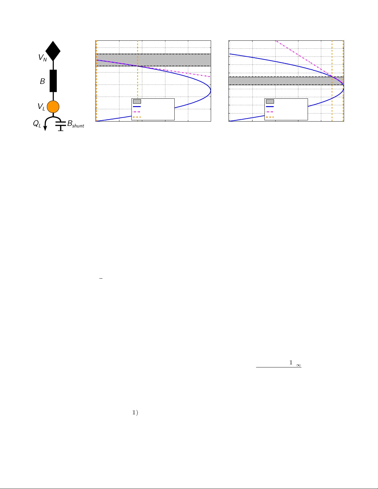
V oltage str ess minimization by optimal r eactiv e power contr ol Marco T odescato, John W . Simpson-Porco, Florian D ¨ orfler , Ruggero Carli and Francesco Bullo Abstract —A standard operational requirement in power sys- tems is that the voltage magnitudes lie within prespecified bounds. Con ventional engineering wisdom suggests that such a tightly-regulated profile, imposed for system design purposes and good operation of the network, should also guarantee a secure system, operating far from static bifurcation instabilities such as voltage collapse. In general howe ver , these two objectiv es are distinct and must be separately enfor ced. W e formulate an optimization problem which maximizes the distance to voltage collapse through injections of reactiv e power , subject to power flow and operational voltage constraints. By exploiting a linear approximation of the power flow equations we arrive at a con vex r eformulation which can be efficiently solved f or the optimal injections. W e also address the planning problem of allocating the resour ces by recasting our problem in a sparsity- promoting framework that allows us to choose a desired trade- off between optimality of injections and the number of requir ed actuators. Finally, we present a distributed algorithm to solve the optimization problem, showing that it can be implemented on-line as a feedback controller . W e illustrate the performance of our results with the IEEE30 bus network. Index T erms —power networks, voltage support, r eactive po wer compensation, resource allocation, distributed control. I . I N T R O D U C T I O N T raditionally , the main purpose of voltage support is to maintain voltage magnitudes tightly within predetermined se- curity constraints (e.g., within 5% of some nominal level). Con ventional wisdom suggests that such a tightly regulated voltage profile, imposed for system design reasons and good operation of the po wer network, should also guarantee a secure system, operating far from static bifurcation instabilities such as v oltage collapse. T echniques for voltage support include shunt and static V AR compensation [1], series compensation [2], off-nominal transformer tap ratios [3], synchronous con- densers [4], and inv erters operating away from unity power factor [5]. See [6] for a survey on the topic. A distinct v oltage control problem, which represents a key direction in po wer system stability analysis, has been the dev elopment of indices quantifying a power network’ s proximity to voltage collapse. A broad ov erview of this large subfield can be found in [7], [8], [9]. The most reliable existing approaches are largely based on numerical methods and lack detailed theoretical support. They often require either continuation power flow [10] to identify the insolv ability This work was supported by the Ing. Aldo Gini Foundation, Padov a and by the ETH start-up funds. M. T odescato and R. Carli are with the Department of Information Engineering, Uni versity of Padov a { todescat|carlirug } @dei.unipd.it . J. W . Simpson-Porco is with the Department of Electrical and Computer Engineering, Uni versity of W aterloo jwsimpson@uwaterloo.ca . F . Bullo is with the Depart- ment of Mechanical Engineering and the Center for Control, Dynami- cal System and Computation, Univ ersity of California at Santa Barbara bullo@engineering.ucsb.edu . F . D ¨ orfler is with the Automatic Con- trol Laboratory , Swiss Federal Institute (ETH) Zurich dorfler@ethz.ch . boundary , or repeated computation of loading margins ov er various directions in parameter-space [11]. As stressed, voltage support and distance to collapse are often analyzed separately in power systems although they are intrinsically related through the well known principle of reac- tiv e power injection. Combining the two problems represents the first contribution of the paper which is threefold. Indeed the ultimate goal in voltage support problems is the security task to confine the voltage magnitudes within predetermined bounds, as suggested by con ventional engineering wisdom. Here, we follow an alternati ve approach: we define a particular measure for the network stress , i.e., the stress experienced by the network induced by the load profile. In particular , we begin our analysis from the recent article [12] where a sufficient and tight condition was presented for solvability of decoupled reactive power flow . This condition, rigorously prov ed only for the reactive decoupled case, quantifies the proximity to voltage collapse by determining a nodal measure of network stress. Based on this condition we pursue a novel system-lev el formulation of optimal voltage support encoded as an optimization problem with str ess-minimization , i.e., max- imization of the distance to voltage collapse, as objective and subject to voltage security constraints. This approach allows us to match a local security requirement as well as a system- level stress-minimization objectiv e encoding the distance to collapse. By exploiting an opportune linearized reformulation, our optimization formulation becomes con vex and can be efficiently solv ed for the optimal injections. As second contri- bution, we also address the planning problem of allocating the av ailable resources by regularizing our optimization problem with a con vex proxy of the cardinality function. This sparsity- promoting formulation allows us to choose a desired trade- off between performance and a cost-ef fectiv e solution. Finally , we present a distributed algorithm for the stress minimization problem which is amenable to real-time implementation as a distributed feedback controller . Compared to other approaches to voltage support problems our results do not rely on the assumption of a radial (i.e., acyclic) po wer grid topology [5]. This makes our approach appealing for po wer transmission networks. Different from the reactiv e power compensation literature [13] and from the voltage support literature [5], we seek stress minimization rather than optimal power flow (minimizing, e.g., losses) or voltage security tasks. Moreover , our formulation can nicely incorporate controller placement tasks. The remainder of this paper is or ganized as follows. In Section II we introduce the required power system model. In Section III we present the first two main contributions of the paper: (i) we revie w the typical objectiv es for voltage regula- tion problems, propose a novel measure for the network stress, and formulate our optimization problem. W e then present and solve the con vex reformulation of the problem. (ii) W e analyze a sparsity-promoting cost to address the planning problem. In Section IV we present the third contribution consisting in a distributed strategy to perform real-time stress minimization. Finally , Section V offers conclusions and future directions. I I . P R E L I M I N A R I E S A. P ower Network, Generator and Load Models A high voltage power network can be modeled as a connected, undirected and complex-weighted graph G ( V , E ) where V = { 1 , . . . , n } represents the set of nodes (or buses ), E ( |E | = m ) is the set of edges (or branc hes ) connecting the nodes, that is the set of unordered pairs ( h, k ) , h, k ∈ V , such that h and k are connected to each other . Under synchronous steady-state operating conditions, all the electric quantities are sinusoidal signals at the same frequency . At e very bus h ∈ V we ha ve the following phasor quantities: • nodal voltage: u h = V h exp(j θ h ) ∈ C ; • current injection: i h = I h exp(j ψ h ) ∈ C ; • power injection: s h = p h + j q h = v h i h ∈ C ;. where V h , θ h , I h , ψ h , p h , q h ∈ R and ( · ) denotes the complex conjugate operator . By collecting all quantities into vectors u, i, s ∈ C n , Kirchhof f ’ s and Ohm’ s laws lead to i = j B u , (1) where j denotes the imaginary unit. The symmetric and sparse susceptance matrix B ∈ R n × n encodes the topology of the underlying electric netw ork weighted by the line susceptances. Follo wing standard assumptions we neglect line losses in high- voltage transmission networks [14], [15]. For recent studies on lossy distribution networks, see [5], [13]. From (1) we can write the P ower Flow Equations (PFEs) as s = [ u ] i = [ u ](j B u ) , (2) where [ x ] denotes the diagonal n × n matrix with diagonal entries x i . Expanding (2), for each h ∈ V the real and imaginary parts must satisfy p h ( u ) = X n k =1 B hk V h V k sin( θ h − θ k ) , (3a) q h ( u ) = − X n k =1 B hk V h V k cos( θ h − θ k ) . (3b) The PFEs (3a)–(3b) relate the voltage v ariables ( θ , V ) to the power variables ( p, q ) , while the behavior of each bus is specified by the particular model assumed to describe it. In this paper , we partition the set of buses V into two subsets, namely V L ( |V L | = n ` ) which identifies power-r egulated or load b uses, and V G ( |V G | = n g ) which identifies voltage- r egulated buses. 1 In particular , we assume the following: • V olta ge-r egulated bus model : voltage-regulated buses are modeled as standard P V buses [14]. This model is widely used, e.g., for generators in transmission grids and micro- generators used for reactive power control in (micro) distribution grids [16]. 1 W e use the subscript G for voltage-re gulated buses because in transmission grids these are typically generator buses. • Load bus model : loads are modeled as P Q buses [15], [17]. In our setup, this model refers also to sources interfaced with power electronics and voltage support equipment such as synchronous condensers. While our results extend to ZIP load models [14], for simplicity of presentation we restrict ourselves to constant power loads q h ( u ) = Q h ; constant impedance loads can be incorporated into the B matrix as diagonal elements. After relabeling the buses to place loads before generators, the matrix B can be partitioned in the block-matrix form B =  B LL B LG B GL B GG  . (4) Assumption 1 (Pr operties of B LL ): (i) B LL is a Metzler matrix whose eigen values are charac- terized by a negati ve real part; 2 (ii) the graph associated to the B LL matrix (i.e., the graph induced by the load buses V L ) is connected. Assumption 1 (i) is typically verified in practice [18], and always satisfied in the absence of phase-shifting transformers, line-charging and shunt capacitors. Regarding the shunt ca- pacitors, they are allowed to be different from zero, howe ver Assumption 1 (i) limits their sizes. Assumption 1 (ii) can be made without loss of generality , since connected components of the induced graph will be electrically isolated from one another by voltage-regulated generator buses. B. Decoupled Reactive P ower Flow & Critical Load Matrix Under normal operating conditions, the high-voltage operat- ing point is characterized by small v oltages angle differences [15] which are treated as parameters [18] or considered as neg- ligible [19]. W e formalized this statement with the following Assumption 2 (Decoupling Assumption): In steady- state operating conditions, for δ ∈ [0 , π / 2[ , the voltage angle differences are constant and such that | θ h − θ k | ≤ δ , ∀ ( h, k ) ∈ E . Note that, under Assumption 2, from the form of Eq.(3b), it is possible to define an effective susceptance matrix by embed- ding the power angle terms into the original line susceptances. Under the decoupling Assumption 2 the Reactiv e Power Flo w Equations (RPFEs) (3b) simplifies in vector notation to q ( V ) = − [ V ] B V . (5) W e now take into account the models and the partition introduced in Sections II-A and, accordingly we partition the vectors of v oltage magnitudes and reactive power injections as V =  V T L V T G  T , Q =  Q T L Q T G  T . Combining the power flow (5), the loads model and the partitioning (4), the power balance Q h = q h ( V ) at each load h ∈ V L can be written as Q L = − [ V L ] ( B LL V L + B LG V G ) . (6) W e define the open-circuit voltages V ∗ L as V ∗ L := − B − 1 LL B LG V G , (7) 2 In other words, B LL is an M -matrix. V N V L B shunt B Q L (a) Example system. 0 0.2 0.4 0.6 0.8 1 0 0.2 0.4 0.6 0.8 1 1.2 No r ma li z ed lo a din g Q L /Q cr i t Loa d vol t age V L Security set Voltage solutions Sensitivity Allowed load (b) Absence of shunt. 0 0.2 0.4 0.6 0.8 1 0 0.2 0.4 0.6 0.8 1 1.2 1.4 1.6 1.8 2 N or m a l i z e d l oa d i n g Q L / Q c r i t L oad v ol t a ge V L Security set Voltage solutions Sensitivity Allowed load (c) Presence of shunt. Fig. 1: T wo-b uses case: panel (a) plots the network scheme where V N = 1 [p . u . ] , B = 4 S . Panels (b)–(c) plot the QV nose curve for two different configurations: (a) Absence of shunt capacitor , B shun t = 0 . (b) Presence of shunt capacitor, B shun t = 2 . 4 S . which are well defined under Assumption 1. Physically , the open-circuit voltages (7) are the voltages one would measure at the load buses for zero reactiv e power demands Q L = 0 n ` . W ith this notation, the RPFEs (6) can be written as Q L = − [ V L ] B LL ( V L − V ∗ L ) . (8) Once (8) is solved for an operating point V L , the reactiv e power injections at generators b uses V G are uniquely deter - mined by substituting the operating point into the final n g equations in (5). W e define one more useful quantity . Definition 3 (Critical Load Matrix): Giv en the matrix B LL and the open-circuit profile V ∗ L as defined in (7), the critical load matrix Q crit is defined as Q crit := 1 4 [ V ∗ L ] B LL [ V ∗ L ] . (9) The critical load matrix Q crit concisely combines the net- work structure, generator voltages, shunts, and the relati ve locations of generation and load. In particular , it will help us to formulate the optimal voltage support problem to follow . Finally , it is conv enient to rewrite (8) in a normalized set of variables. Using the open-circuit voltages V ∗ L defined in (7), we denote the vector of normalized voltages as v := [ V ∗ L ] − 1 V L . (10) Note that if the open-circuit profile is flat ( V ∗ L = α 1 for some α > 0 ), then v is simply the standard vector of per unit voltages. In general, ho wev er, due to inhomogeneous generators voltage set points and the presence of shunt com- pensation, V ∗ L is not flat and the scalings in (10) are non- uniform. Substituting V L = [ V ∗ L ] v into the RPFEs (8) and using (9), (8) takes the simple form Q L = − 4[ v ] Q crit ( v − 1 ) . (11) I I I . F O R M U L AT I O N O F O P T I M A L V O L TAG E S U P P O RT P RO B L E M In this section we present our novel problem formulation. First, we present a common operational requirement highlight- ing its possible inadequac y to capture the safe operation of the grid. Then, we present a novel metric to measure the stress induced on the network by the load demand, representing our objectiv e function. Finally , we present a linearization which leads to a con ve x reformulation of the optimization problem. A. Security Constraints A common operational requirement is that the load b uses voltage magnitudes must lie within a predefined percentage deviation, typically 5% , from a reference voltage. This tight clustering of voltages is due to the follo wing reasons: (i) loads and some system components are designed to operate with a voltage in a narro w region around the network base voltage; (ii) a flat voltage profile minimizes current flows and, con- sequently , minimizes resistiv e power losses; (iii) a flat profile usually reduces the sensitivity of the voltage profile with respect to load changes (see Example 5); (iv) most importantly , by conv entional wisdom (see typical nose curve studies [9], [14]) a flat voltage profile indi- cates that the network is safe from voltage collapse. W e formalize this requirement by defining the secure set . Definition 4 (Secure set): Given a reference voltage V N ∈ R > 0 , a percentage deviation α > 0 and V ∗ L as in (7), the secur e set V α is defined as V α :=  v ∈ R n `    k [ V ∗ L ] v − V N 1 k ∞ V N ≤ α  . (12) Hence, if v ∈ V α is a solution to (11), then all voltages lie within α percent of the nominal v oltage V N . While this represents a baseline operational requirement, under some circumstances it may not be suf ficient to ensure safe grid operation. W e present a simple example highlighting this fact. Example 5 (Security r equir ement inadequacy): Consider the simple two-buses case study consisting of a load connected to a source at voltage V N = 1 , as illustrated in Figure 1a. For the case where B shun t = 0 , Figure 1b plots the nose curve , i.e., the locus of solutions to (8) (blue solid blue) as Q L is varied from 0 to Q crit . Note that for a chosen Q L , there may be two, one, or zero feasible solutions of (8). The secure set is shown as a shaded area between two dashed black lines. Also shown are the loading limits which ensure the high-voltage solution to lie in the secure set (dashed orange), and the tangent line to the nose curv e at the mid-point between the dashed orange lines (dashed magenta). This tangent line captures the sensiti vity of the load v oltage to changes in reactiv e po wer demand. From Figure 1b, note that if Q L is too large, the operating point does not lie within V α . A standard policy is then to support the voltage level by adjusting the shunt compensation, i.e., by increasing B shun t . When B shun t = 0 , Figure 1b demonstrates that the security requirement v ∈ V α guarantees a “safe” distance to collapse, represented by the nose of the blue curve. Moreov er, the sensitivity of the voltage to changes in load is small, meaning that relativ ely lar ge changes in loading do not translate into large voltage changes. Con versely , in Figure 1c B shun t 6 = 0 , and the security requirement v ∈ V α is “dangerously” close to the nose of the curve. Finally , the sensitivity line is steeper meaning that small changes in the load cause relatively big changes in the voltage. This affects the robustness of the network to small load changes.  The previous analysis highlights that the security require- ment v ∈ V α alone could be insufficient. Note that, to operate the grid in the point farthest from v oltage collapse and to ultimately maximize the stability and robustness mar gins, a simple intuition is that of minimizing the distance of the operating point from the open-circuit solution V ∗ L , represented by the left-most point on the blue curv e — constrained to the fact that the operating point must belong to V α . As final remark, note that in general V ∗ L does not belong to V α . Thus in general, distance-to-collapse minimization and v oltage compensation do not coincide. B. Network Str ess Measur e and Stress Minimization Problem Based on the insights given by Example 5, we define the following measure quantifying the distance to collapse. Definition 6 (Network Str ess Measur e): Consider the RPFEs (11) in the normalized voltages v ∈ R n ` . The network str ess measure induced by the load is defined as J stress ( v ) := k v − 1 k ∞ . (13) Definition 6 is based on the intuition that the open-circuit profile V ∗ L is the network’ s natural operating point in absence of loading, i.e., under “no stress”. Con versely , when the network works close to the nose tip, i.e., the farthest point from V ∗ L then, this is a “high-stress” scenario. In this sense, the stress function (13) quantifies the loading on the network con- veniently expressed in the normalized profile v = [ V ∗ L ] − 1 V L . In the following, we assume that a certain number of load buses can be equipped with additional controlled devices, e.g., synchronous condensers [4]. W e assume these devices can provide a controllable amount of reactive power support, and in the follo wing we model them as controllable sources of reactiv e po wer q h , subject to upper and lower operational bounds. Specifically , the RPFEs (11) are modified as Q L + q = − 4[ v ] Q crit ( v − 1 ) , (14) where q ∈ R n ` is such that q min ≤ q ≤ q max and q min , q max ∈ R n ` are vectors representing the injection capacity constraints. If load bus h ∈ V L is not equipped with a compensator, we set q min ,h = q max ,h = 0 . W e no w formulate our optimization problem of interest, which we refer to as the Stress Minimization problem. Pr oblem 7 (Str ess Minimization): Given Q L , Q crit as in (9) and the capacity limits q min , q max , find q and v such that minimize q ∈ R n ` J stress ( v ) , (15) sub ject to      v ∈ V α , q min ≤ q ≤ q max , Q L + q = − 4[ v ] Q crit ( v − 1 ) . The main idea behind Problem 7 is that minimizing J stress keeps the operating point away from the tip of the nose curve, i.e., the collapse point. The standard security requirement v ∈ V α is imposed as a hard constraint. Since v is related to q through the quadratic equality constraints (14), Problem 7 is nonlinear and non-con ve x. In the following, we con ve xify this problem through the use of a po wer flow linearization. C. Linear Appr oximation and Con vexification W e no w introduce a suitable linearization for Problem 7 which had been first presented in [20]. From (14), assuming k Q L + q k ∼ 0 , we expect the normalized profile (10) to be v ' 1 which would be the e xact high voltage solution corresponding to Q L + q = 0 . Linearizing the RPFEs (14) around v = 1 , to first order , the solution is giv en by b v = 1 − 1 4 Q − 1 crit ( Q L + q ) . (16) That is, to first order the solution of (14) is gi ven by a uniform component plus a deviation which is linear in the reactiv e injections. Using (16), the cost (13) is approximated by J stress ( v ) = k v − 1 k ∞ ∝   Q − 1 crit ( Q L + q )   ∞ . (17) Note that the approximated cost function (17) is con ve x in the reactive po wer injections q . By exploiting (16) and thanks to some algebraic manipulations, it is possible to see that the security requirement b v ∈ V α holds if and only if V N (1 − α )[ V ∗ L ] − 1 1 ≤ b v ≤ V N (1 + α )[ V ∗ L ] − 1 1 . (18) Substituting for b v from (16), (18) is equi v alent to ξ min ≤ − Q − 1 crit q ≤ ξ max , (19) where ξ min := 4  V N (1 − α ) [ V ∗ L ] − 1 1 − 1  + Q − 1 crit Q L , (20a) ξ max := 4  V N (1 + α ) [ V ∗ L ] − 1 1 − 1  + Q − 1 crit Q L . (20b) Thus, the security constraints b v ∈ V α hav e been con verted into linear inequality constraints on the decision variables q . W e now present the conv exified version of Problem 7. Pr oblem 8 (Con vex Stress Minimization): Consider the RPFEs (14). Let Q crit be as in (9) and q min , q max be vectors (a) γ = 0 (b) γ = 4 × 10 − 4 (c) γ = 8 × 10 − 4 Fig. 2: Placement scheme of the compensation devices for different values of γ . Black diamonds ♦ represent generators, circles  represent loads, and triangles 5 represent reactive compensators. Color scheme: red scale − represents increasing power absorption; blue scale − represents increasing power injection. representing the injection capacity limits. Finally , define ξ min and ξ max as in (20a)–(20b), respectiv ely . Then the goal is to minimize q ∈ R n `   Q − 1 crit ( Q L + q )   ∞ , (21) sub ject to ( ξ min ≤ − Q − 1 crit q ≤ ξ max , q min ≤ q ≤ q max . (22) Remark 9 (On the str ess measure): Aside from the linearization-based deriv ation in this subsection, the measure (21) is inspired by recent results [12] on the solv ability of the decoupled reacti ve power flo w equations (8), where it has been sho wn that k Q − 1 crit Q L k ∞ represents a proper distance-to-collapse measure. Indeed, if k Q − 1 crit Q L k ∞ < 1 , the non linear (8) has a unique high-voltage solution safe from collapse.  Observe that in Problem 8 the cost (21) and the constraints (22) are conv ex in the decision v ariables. Moreover , Problem 8 can be written as a linear program and can therefore be efficiently solved via con vex optimization. Before presenting some performance and simulations of the stress minimization procedure, notice that both Problems 7 and 8 are offline centralized procedures which, as suggested by the formulation in Section III-B, assume that either the full set of load buses or only an a priori assigned subset of them are equipped with controllable devices. The first scenario is impractical and economically unfeasible in large networks due to the large number of devices needed. The second scenario could likely lead to a sub-optimal allocation of resources if no specific allocation policies are used. In the follo wing subsection, we refine Problem 8 to simultaneously solve for the planning problem of allocating the resources along with the system-le vel stress minimization problem. D. The Planning Pr oblem: Sparse Stress Minimization Here we propose a modification of Problem 8 to find a desired trade-off between the number of actuators and the minimization of the stress cost. In order to accomplish this task, we propose a sparsity-pr omoting approach where, by tuning an additional parameter , the user is able to control the sparsity of the solution. In this way , we simultaneously solve the system-level stress minimization problem as well as the planning problem of allocating a finite number of resources. The cardinality function, card( · ) , is a natural choice to ac- count for the number of devices. Howe ver , it is discontinuous and non-con vex. A con vex approximation of card( q ) is the r e-weighted ` 1 -norm [21] k [ w ( q )] q k 1 = n ` X h =1 w h ( q h ) q h , w h ( q h ) := 1 | q h | +  , (23) where 0 <   1 . Adding equation (23) to the cost function (21), it is possible to formulate the following problem which we refer to as the Sparse Stress Minimization problem. Pr oblem 10 (Sparse Stress Minimization): Consider the same set-up as in the Con ve x Stress Minimization of Problem 8. Then the goal is to minimize q ∈ R n `   Q − 1 crit ( Q L + q )   ∞ + γ k [ w ( q )] q k 1 , (24) sub ject to ( ξ min ≤ − Q − 1 crit q ≤ ξ max , q min ≤ q ≤ q max . The parameter γ in the cost function (24) can be used to promote sparsity of the solution q , and thereby minimize the number of required actuators. Obviously for γ = 0 , Problem 10 reduces to Problem 8. By increasing the value of γ the user can force the solver to lean tow ards a more sparse solution. This automatically compels the solver to optimally allocate the resources in order to find the best trade- off between sparsity and system-lev el stress minimization. E. Simulation: Planning Pr oblem and Offline Optimization W e now present a case study to show the ef fectiv eness of planning and the of fline optimization procedure proposed. The simulations refer to Problem 10 and are implemented in MA TLAB and CVX [22]. The plotted voltage profiles refer to the linearized solution (16) of the decoupled RPFEs (14). The test-bed consists of: • IEEE 30 bus transmission grid [23]; 0 0.1 0.2 0.3 0.4 0.5 0.6 0.7 0.8 0.9 1 x 10 −3 0 5 10 15 20 25 γ # D e v i c e s 0 0.1 0.2 0.3 0.4 0.5 0.6 0.7 0.8 0.9 1 x 10 −3 0 20 40 60 80 100 C o s t : p o s t / p r e [ % ] Fig. 3: Behavior of the number of devices (left-blue axis) and of the ratio of the cost value after and before the optimization (right-red axis) as function of the sparsity parameter γ . • a reference voltage V N = 1 [p.u.]; • a voltage deviation limit α = 5% ; • capacity limits { q min , q max } = {− 0 . 5 , 0 . 5 } × k Q L k ∞ 1 . Figures 2a–2b–2c illustrates the placement of actuators for increasing values of γ ( γ = 0 , γ = 4 × 10 − 4 and γ = 8 × 10 − 4 , respectively). Compensators placed by the optimization problem are indicated with a triangle. The color scheme for loads Q L and compensators q is as follows: • reactiv e injections, i.e., positi ve values, are plotted in blue-scale ( − ): the lighter the blue, the bigger the injection absolute value; • reactiv e consumptions/absorptions, i.e., negati ve values, are plotted in red-scale ( − ): the darker the red, the bigger the absolute value of the consumption; • white node means zero injections/consumptions. First of all, for γ = 0 the solver places compensation ev erywhere. Moreov er it can be seen that one compensator is red colored, meaning that it effecti vely absorbs reactiv e power . This occurs due to large reactiv e po wer injections at neighboring buses, which driv e up voltage values across the network – additional reactiv e power must be absorbed to lower specific voltages and meet the security constraints. Sparsity promotion takes place for increasing γ with the solver placing compensators only where the heaviest loading occurs. Figure 3 shows, as a function of γ , the number of devices placed (left- blue axis) and the ratio between the value of the cost (21) after a polishing step, i.e., obtained as solution of Problem 8 given the placement obtained solving Problem 10, over the value of the cost before the optimization (right-red axis), i.e., k Q − 1 crit ( Q L + q ) k ∞ k Q − 1 crit Q L k ∞ . It can be seen how , for increasing γ the final value of the cost increases since a smaller number of controllable units are less able to compensate the voltage profile. Howe ver , as can be seen from the first part of the plot, by using only 11 controllers we achie ve the same performance as of using 24 compensators. This not only highlights the redundancy of using 24 compen- sators but that the optimal placement is necessary to achiev e the same level of performance. Figures 4 shows the linearized profiles of V L before and after the optimization for different γ . It can be seen that for increasing γ the profile V L is less Bus Numb e r 0 5 10 15 20 25 V oltage [p. u.] 0.85 0.9 0.95 1 1.05 V N V $ L V L before opt : V L after opt : : . = 0 V L after opt : : . = 0 : 00055 V L after opt : : . = 0 : 001 Security b ound Fig. 4: V oltage profiles for different values of γ . compensated, i.e., it is farther from the V ∗ L profile. Finally , as already stressed, note that stress minimization and classical voltage compensation do not coincide. Indeed, V ∗ L , in general, does not belong to V α , identified by the black dashed lines. I V . D I S T R I B U T E D O N L I N E S T R E S S M I N I M I Z AT I O N T H RO U G H F E E D B AC K C O N T RO L The previous methods of Sections III-C and III-D are suitable only for offline optimization and planning. In this section we assume the planning problem has been solv ed offline, and de velop a dual-ascent algorithm for Problem 8 which may be implemented online as a distributed feedback controller . This is motiv ated by different reasons among which it is worth mentioning that: • utilities could prefer not to share information with a central operator because of priv acy reasons; • an online implementation can be naturally exploited as a distributed feedback controller in presence of time- varying loads, to reject disturbances, to increase the system rob ustness, and to track the optimal solution. In the follo wing, we assume that “smart agents” are embedded at all the grid’ s load buses. These are characterized by mild communication and computational capabilities. Moreov er, they can communicate according to a communication graph which is designed to coincide with the electrical network. It is worth mentioning that, as will be clear later , e ven the load buses not equipped with a controllable compensator are required to share “smartness” capabilities. In the current formulation of Problem 8, the presence of the dense matrix Q − 1 crit in both the cost J stress and the constraints (19) compromises the possibility to solve the stress minimization problem in a distributed fashion. Howe ver , the matrix Q crit is sparse and the graph induced by its sparsity pattern coincides with the topology of the grid which connects the load buses. W e take advantage of this structure to dev elop a distrib uted algorithm to solve Problem 8. Whereas the formulation of Problem (8) expressed the stress minimization compactly in injection coordinates q , no w we deriv e the equi v alent formulation in voltage coordinates to lev erage on the sparsity of Q crit . W e start our analysis defining the deviation variable x as x := − Q − 1 crit ( Q L + q ) , (25) which represents the linear de viations of the v oltages b v as defined in (16) due to the ov erall reactiv e injection. Similar to what done in Section III-C, from the definition of set V α it is possible to obtain the security constraints expressed in the x coordinates. These are equal to x min ≤ x ≤ x max , where x min := 4  V N (1 − α ) [ V ∗ L ] − 1 1 − 1  , x max := 4  V N (1 + α ) [ V ∗ L ] − 1 1 − 1  . From the definition of x it is clear that q = − ( Q crit x − Q L ) . (27) Since the matrix Q crit is characterized by a sparsity pattern equiv alent to that induced by the electric graph connecting the loads, the desired control inputs can be computed by means of a local exchange of information, namely the x i variables among electric neighbors. Additionally , from (27) it is easy to impose the capacity constraints, i.e., q min ≤ q ≤ q max . The Problem 8 is then equiv alent to Pr oblem 11 (Online Stress Minimization): minimize x ∈ R n ` k x k ∞ , (28) sub ject to ( x min ≤ x ≤ x max , q min ≤ − ( Q crit x − Q L ) ≤ q max . Now , we point out three more issues related to Problem 11: (i) the ∞ -norm is not ev erywhere dif ferentiable and thus not suitable for a gradient-based iterativ e procedure; (ii) comput- ing the cost in (28) requires knowledge of all x i variables; (iii) in order to compute the deriv ativ e of the maximum function embedded in k · k ∞ , the index where the maximum is attained must be known. Next, we propose one possible solution to these issues. A. A Smooth Decomposable Approximation of ∞ -norm W e now present a continuously dif ferentiable approximation for the ∞ -norm which combines a smooth approximation for the maximum function, the softmax [24], and a smooth approximation for the absolute value. This reads as ˜ f α, ( x ) := softmax α ( | x | 1+  ) , 1  α , 0 <   1 , = 1 α log  1 n ` X n ` i =1 exp  α | x i | 1+    . (29) The idea behind (29) is to exploit the super-linearity property of the exponential to let the maximum component of the vector x dominate the other components. The exponentiation is exploited to recover differentiability of the absolute value. The approximation ˜ f α, ( x ) approximates k x k ∞ in the following sense; the proof can be found in Appendix A. Lemma 12 (Limit behavior of ˜ f α, ): Consider ˜ f α, as in (29). Then, it holds that lim α → + ∞  → 0 + ˜ f α, ( x ) = k x k ∞ . Now , let us define f α, ( x ) := n ` exp( α ˜ f α, ) = n ` X i =1 exp( α | x i | 1+  ) . (30) Notice that, due to the monotonicity of the log function in the softmax, it holds that argmin x ∈ R n ` ˜ f α, ( x ) ≡ argmin x ∈ R n ` f α, ( x ) . (31) Thanks to this simplification and in view of the distrib uted implementation, notice that the i -th component of the gradient vector of (30) is equal to ∂ f α, ( x ) ∂ x i = α (1 +  ) exp( α | x i | 1+  ) | x i |  sgn( x i ) , (32) which depends only on the local state x i of agent i . W e will exploit this fact in our reformulation of Problem 11. The following lemma — whose proof may be found in Appendix B — characterizes the con ve xity of f α, ( x ) . Lemma 13 (Str ong con vexity of f α, ): Consider the func- tion f α, : R n ` 7→ R defined as in (30). Then, for all 0 <  ≤ 1 and for all α > 0 , f α, is strongly conv ex in x . While Lemma 12 provides an asymptotic result, one finds that numerical issues are encountered for sufficient large (resp., small) values of α (resp.,  ). In practice howe ver , reasonably small v alues of α (resp.,  ) provide excellent results, with no noticeable numerical issues. B. A Distributed Primal-Dual F eedback Contr oller W e now reformulate Problem 11 by exploiting (30) and the equiv alence in (31). By introducing the additional quantities I :=  I − I  , χ :=  x max − x min  , ϕ :=  q max − q min  , (33) the smooth approximation of Problem 11 reads as Pr oblem 14 (Smooth Stress Minimization): minimize x ∈ R n ` f α, ( x ) , (34) s . t . ( I x ≤ χ , I ( Q crit x − Q L ) ≤ ϕ . where, thanks to (33), the constraints are now in the standard form of a con ve x program. One possible way to solve Problem 14 is the use of standard dual-ascent discrete-time algorithm [25]. The Lagrangian func- tion associated to (14) is equal to L ( x, λ, µ ) = f α, ( x ) + λ T ( I x − χ ) + µ T ( I ( Q crit x − Q L ) − ϕ ) , where λ, µ ∈ R 2 n ` are vectors of Lagrange multipliers. The dual-ascent then consists of the iterati ve updates x ( t + 1) = argmin x L ( x, λ ( t ) , µ ( t )) , (35a) λ ( t + 1) = [ λ ( t ) + ρ ( I x ( t + 1) − χ )] + , (35b) µ ( t + 1) = h µ ( t ) + ρ ( I ( Q crit x ( t + 1) − Q L ) − ϕ ) i + (35c) where ρ > 0 is the step size and [ · ] + denotes the projection on the positiv e orthant, that is, [ a ] + = a, if a > 0 , and 0 GRID Controller (load i ) z -1 q i (t) y i (t) q i (t+1) x j ,µ ji x i ,µ ij Controller (load j ) q j (t) q j (t+1) z -1 y j (t) Fig. 5: Illustration of distributed control architecture. Measurements y ( t ) are gathered from the grid and used, together with q ( t ) , to update x . Neighboring controllers exchange information. The block z − 1 is the one-step delay operator . otherwise. W e no w state a con vergence result whose proof can be found in Appendix C. Pr oposition 15 (Con verg ence of the dual ascent algorithm): Consider Problem 14 and assume that Slater’ s condition holds, namely , a strictly feasible solution for (34) exists. Then, there exists ρ such that for any ρ ≤ ρ , the dual ascent algorithm (35) con verges to the optimal solution of (34). Observe that the desired control injections can be computed by the corresponding agents from (27) as q ( t + 1) = − ( Q crit x ( t + 1) − Q L ) . (36) From (35), one can see that the proposed dual ascent algorithm is amenable of distributed implementation meaning that node i , to compute x i ( t +1) , µ i ( t +1) , needs only information coming from neighboring nodes (with the sparsity pattern induced by the Q crit matrix); while no exchange of information is needed to compute λ i ( t + 1) . T o be more precise, observe that (35a) is separable in the x i variable; indeed, from the first order optimality condition must hold for any i ∈ V that ∂ ∂ x i L ( x, λ ( t ) , µ ( t )) = 0 , which is equiv alent to ∂ f α, ( x ) ∂ x i = − X j ∈N i  [ I T ] ij λ j ( t ) + [ Q crit I T ] ij µ j ( t )  | {z } ζ i ( t ) , (37) where N i := { j ∈ V : [ Q crit ] ij 6 = 0 } represents the set of neighbors of node i . Observe that the right hand side of (37) is constant giv en the multipliers of the neighbors and that, thanks to strong con vexity of f α, and monotonicity of its first deriv ativ e, (37) has always a unique real-valued solution. Interestingly , for  = 1 a closed-form solution for (37) exists and is equal to x i ( t + 1) = sgn( ζ i ( t )) 1 √ 2 α s W  ζ 2 i ( t ) 2 α  , (38) where W ( · ) is the Lambert W or ProductLo g function [26] defined as the in verse of the function g ( z ) = z exp( z ) . Finally , 0 2 4 6 8 10 x 10 5 −0.35 −0.3 −0.25 −0.2 −0.15 −0.1 −0.05 0 I t e r a t i o n s L o a d s Q L [ M V a r ] Fig. 6: Dynamics of the loads Q L . The different colored curves represent the time ev olution of the loads at different buses. note that, each agent needs to know some model information, namely its corresponding Q crit entries which are related to the electric quantities connecting them to their neighbors. It is worth noticing the presence of the load demand Q L in both (35c) and (36). Usually , it is reasonable to have voltage and current monitoring at each bus. From this measurements it is possible to extract information about the total reacti ve load absorbed or injected at the bus. In particular, by defining y := Q L + q as the aggregate contribution of the load together with the control input, from the bus monitoring it is possible to measure y rather than Q L independently . In order to compute (35c) and (36) it is suf ficient to set Q L = y ( t ) − q ( t ) , where y ( t ) and q ( t ) are the aggregate load measurements and the control input at the current t iteration. An illustration of the control loop is showed in Figure 5: the aggreg ate measurements are taken from the grid and are used together with the control input to compute the update x ( t + 1) . Then, by using x ( t + 1) , y ( t ) and q ( t ) , the new control input q ( t + 1) , used to actuate the grid, are computed. C. Simulation: Distributed Online F eedback Contr oller W e now present simulations illustrating the effecti veness of our distrib uted controller in the presence of time-v arying loads. The setup is the same as used in Section III-E. Howe ver , differ - ently from the pre vious set of simulations, we simulate the full 0 2 4 6 8 10 x 10 5 −0.05 0 0.05 0.1 0.15 0.2 I t e r a t i o n s I n p u t s q [ M Va r ] Fig. 7: Dynamic of the control inputs q . The different colored curves represent control inputs at different controlled buses. 0 1 2 3 4 5 6 7 8 9 10 x 10 5 0.9 0.95 1 1.05 1.1 I t e r a t i o n s Vo l t a g e V L [ p . u . ] s e c u r i t y b o u n d s V L Fig. 8: Evolution of the voltages corresponding to the coupled nonlinear power flow equations. 0 1 2 3 4 5 6 7 8 9 10 x 10 5 −10 −8 −6 −4 −2 0 I t e r a t i o n s l o g k q ( t ) − q o p t k Fig. 9: Evolution of the norm of the error between the online values of q ( t ) and their optimal value q opt computed offline. coupled system at each iteration of the algorithm by means of MA TPOWER [23]. W e sho w the performance of the algorithm assuming we hav e access to aggreg ate measurements y for a fixed allocation of the resources. Specifically , there are 6 controllable units out of 24 total loads at the load buses number 1, 10, 15, 22, 23 and 24. Moreov er, the controlled injections q are saturated before actuating the electric grid, simulating the fact that they cannot exceed their capacity limits. The loads (activ e and reactive) randomly encounter, at half of the simulation time, a jump equal to 40% of their starting value (see Figure 6). All other parameters are held constant. Figure 7 shows the ev olution of the reactive injection returned by the algorithm. Figure 8 shows the corresponding ev olution of bus voltages under the distrib uted controller (35)– (36). Observ e that the voltage solution of the full coupled PFEs remains within the operational bounds. Moreover , we note that the worst case steady-state difference between the solution of the full coupled PFEs and the linearized solution of the RPFEs given by (14) is of only 1 . 2% . This fact highlights the ef fectiv eness of both the linearization and the control algorithm. Finally , Figure 9 shows the evolution of the error between the values of the injection q ( t ) and the optimal value computed offline q opt as solution of Problem 8, as a function of the iterations, in logarithmic scale. Notice that the value of q computed online con verges to the optimal of fline value e ven after the change in the loads. As a limit, it must be noted that the proposed distributed algorithm requires substantial amount of iteration until con ver gence. V . C O N C L U S I O N S A N D F U T U R E D I R E C T I O N S W e considered the problem of voltage support via reactiv e power injections. Con versely to what suggested by con ven- tional wisdom, we sho wed that the standard local security requirement might be inadequate. Then, we proposed a novel optimization formulation whose cost function encodes the stress e xperienced by the grid, while the security requirements are imposed as constraints. Thanks to recent advances on the solvability and linearization of the reacti ve power flows, the problem becomes linear and con vex and can be efficiently solved. In addition, we addressed the planning problem to solve for the optimal allocation of the resources. Finally , thanks to a suitable reformulation, we presented a distributed algorithm to solve for the stress minimization, which imple- ments a real-time feedback controller and which, as drawback, is characterized by a slow con vergence rate. As future research, relev ant practical applications would be to seek for distrib uted implementation which are faster in the conv ergence rate and employ only communications among compensators. Moreov er, it would be worth exploring our novel formulation, which combines system-le vel stress minimization and local security constraints, with respect to different optimization v ariables. From a power system analysis perspectiv e the ultimate problem remains the analysis of the full coupled power flow equations. A P P E N D I X A. Pr oof of Lemma 12 In the following, we will prov e the result by first taking the limit for α followed by the limit for  . It is easy to show , thanks to a T aylor series expansion of ˜ f α, around  = 0 , that exchanging the order of the limits does not change the result. Consider the function ˜ f α, ( x ) as defined in (29) and let us define | x | 1+  max := max i | x i | 1+  . It is possible to re write ˜ f α, ( x ) = | x | 1+  max + 1 α log  1 n X i exp  α ( | x i | 1+  − | x | 1+  max | {z } ≤ 0 )  . Now , since the exponent in the second term is always < 0 except for the components where the maximum is attained which are exactly equal to 0 , we hav e lim α → + ∞ ˜ f α, = | x | 1+  max . Finally , to conclude the proof, notice that the T aylor series expansion around  = 0 + of | x | 1+  max is equal to | x | max + ∞ X n =1 1 n ! | x | max log n ( | x | max )  n − →  → 0 + | x | max .  B. Pr oof of Lemma 13 T o prove strong conv exity of f α, ( x ) we exploit the second order characterization of strong con ve xity which states that a function is strongly con vex if and only if ∇ 2 x f α, ( x ) − m I is positiv e definite, for some m > 0 . The Hessian of f α, is indeed a diagonal matrix whose i -th diagonal entry is equal to α (1 +  ) exp( α | x i | 1+  ) | {z } > 0   | x i |  | x i | + α (1 +  ) | x i | 2   . Note that, the entire expression can fail to be positi ve only if the second term in the right hand side possibly fails to be positiv e. The only possible point of failure is x i = 0 where we encounter a 0 0 limit. Howe ver , being | x i |  = o ( | x i | ) for any finite value 0 <  ≤ 1 , we hav e that ∂ 2 f α, ( x ) ∂ x 2 i − → | x i |→ 0 + ∞ . Since each diagonal component is bounded below by m i > 0 , defining m := min i m i , we can conclude.  C. Pr oof of Pr oposition 15 First of all, we recall (assuming Slater’ s condition holds) that the duality gap is zero. Hence, solving the primal Problem 14 is equiv alent to solve its dual problem which is defined as maximize λ d ( λ ) := inf x f α, ( x ) + λ T  Ax − b  , (39) s . t . λ ≥ 0 . where A :=  I T ( I Q crit ) T  T and b :=  χ T ϕ T  T . Moreov er , thanks to strong con vexity of f α, , the solution is unique. From Proposition 6 . 1 . 1 in [25] follo ws that d is ev erywhere continuously differentiable. Moreov er ∇ λ d ( λ ) = Ax ∗ λ − b where x ∗ λ := argmin x f α, ( x ) + λ T g ( x ) . In addition, the dual ascent algorithm (35) coincides with a projected gradient [25] applied to (39) which, thanks to Proposition 2 . 3 . 2 in [25], is known to con ver ge, for sufficiently small step sizes, namely 0 < ρ < 2 L = ρ , if ∇ λ d is Lipschitz continuous with Lipschitz constant L . T o prove Lipschitz continuity of ∇ λ d , observ e that it is linear respect to x ∗ λ . Then, we just need Lipschitz continuity of x ∗ λ respect to λ . From the definition of x ∗ λ and thanks to first order optimality condition, it holds that ∇ x f α, ( x ∗ λ ) = − A T λ . By defining ζ := − A T λ and recalling from (32) that each component of ∇ x f is only a function of x i , we have that ∂ f α, ( x ∗ λ ) ∂ x i = ζ i , and it is possible to reduce the analysis to show Lipschitz continuity of the i -th component of x ∗ λ respect to ζ i . Now , by being f α, twice continuously differentiable and thanks to the in verse function theorem, ∂ f α, /∂ x i is in vertible, namely [ x ∗ λ ] i =  ∂ f α, ∂ x i  − 1 ( ζ i ) , its in verse is continuously differentiable, and moreov er ∂  ( ∂ f α, /∂ x i ) − 1  ∂ x i =  ∂ ( ∂ f α, /∂ x i ) ∂ x i  − 1 < 1 m i , where the last inequality holds since f α, is strongly con ve x. Then, x ∗ λ is Lipschitz continuous respect to ζ and so respect to λ being the former a linear function of the latter .  R E F E R E N C E S [1] A. Sode-Y ome and N. Mithulananthan, “Comparison of shunt capacitor, SVC and ST A TCOM in static voltage stability margin enhancement, ” International Journal of Electrical Engineering Education , vol. 41, no. 2, pp. 158–171, 2004. [2] M. Moghavv emi and M. Faruque, “Ef fects of F ACTS devices on static voltage stability , ” in Proceedings of TENCON 2000 , vol. 2, 2000, pp. 357–362. [3] F . A. V iawan, A. Sannino, and J. Daalder , “V oltage control with on- load tap changers in medium v oltage feeders in presence of distributed generation, ” Electric P ower Systems Research , v ol. 77, no. 10, pp. 1314– 1322, 2007. [4] G. Andersson, “Modelling and analysis of electric po wer systems, ” 2008, Lecture 227-0526-00, EEH-Power Systems Laboratory , Swiss Federal Institute of T echnology (ETH), Z ¨ urich, Switzerland. [5] L. Na, Q. Guannan, and M. Dahleh, “Real-time decentralized voltage control in distribution networks, ” in Allerton Conf. on Communications, Contr ol and Computing , Monticello, IL, USA, Sep. 2014, pp. 582–588. [6] J. Dixon, L. Moran, J. Rodriguez, and R. Domke, “Reactive power compensation technologies: State-of-the-art revie w , ” Proceedings of the IEEE , v ol. 93, no. 12, pp. 2144–2164, 2005. [7] T . V an Cutsem, “V oltage instability: phenomena, countermeasures, and analysis methods, ” Proceedings of the IEEE , vol. 88, no. 2, pp. 208–227, 2000. [8] C. Ca ˜ nizares, “V oltage stability assessment: Concepts, practices and tools, ” IEEE Power System Stability Subcommittee, T ech. Rep. PES- TR9, 2002. [9] T . V an Cutsem and C. V ournas, V oltage Stability of Electric P ower Systems . Springer, 1998. [10] I. A. Hiskens and R. J. Davy , “Exploring the power flow solution space boundary , ” IEEE T ransactions on P ower Systems , vol. 16, no. 3, pp. 389–395, 2001. [11] I. Dobson and L. Lu, “Computing an optimum direction in control space to av oid stable node bifurcation and voltage collapse in electric power systems, ” IEEE T ransactions on Automatic Control , vol. 37, no. 10, pp. 1616–1620, 1992. [12] J. W . Simpson-Porco, F . D ¨ orfler , and F . Bullo, “V oltage collapse in complex power grids, ” Nature Communications , Mar . 2015, to appear . [13] S. Bolognani, R. Carli, G. Cavraro, and S. Zampieri, “Distributed reactiv e power feedback control for voltage regulation and loss mini- mization, ” IEEE T ransactions on Automatic Control , vol. 60, no. 4, pp. 966–981, 2015. [14] A. R. Bergen and V . V ittal, P ower Systems Analysis , 2nd ed. Prentice Hall, 2000. [15] J. Machowski, J. W . Bialek, and J. R. Bumby , P ower System Dynamics , 2nd ed. John W iley & Sons, 2008. [16] R. H. Lasseter, “Microgrids, ” in IEEE P ower Engineering Society W inter Meeting , v ol. 1, 2002, pp. 305–308. [17] M. K. Pal, “V oltage stability conditions considering load characteristics, ” IEEE Tr ansactions on P ower Systems , vol. 7, no. 1, pp. 243–249, 1992. [18] J. Thorp, D. Schulz, and M. Ili ´ c-Spong, “Reactive power -voltage prob- lem: conditions for the existence of solution and localized disturbance propagation, ” International J ournal of Electrical P ower & Energy Sys- tems , v ol. 8, no. 2, pp. 66–74, 1986. [19] R. Kaye and F . W u, “ Analysis of linearized decoupled power flow approximations for steady-state security assessment, ” IEEE T ransactions on Cir cuits and Systems , vol. 31, no. 7, pp. 623–636, 1984. [20] B. Gentile, J. W . Simpson-Porco, F . D ¨ orfler , S. Zampieri, and F . Bullo, “On reactive power flow and voltage stability in microgrids, ” in Ameri- can Contr ol Confer ence , Portland, OR, USA, Jun. 2014, pp. 759–764. [21] S. Boyd and L. V andenberghe, Con vex Optimization . Cambridge Univ ersity Press, 2004. [22] M. Grant and S. Boyd, “CVX: Matlab software for disciplined con vex programming, v ersion 2.1, ” http://cvxr .com/cvx, Oct. 2014. [23] R. D. Zimmerman, C. E. Murillo-S ´ anchez, and R. J. Thomas, “MA T - PO WER: Steady-state operations, planning, and analysis tools for power systems research and education, ” IEEE T ransactions on P ower Systems , vol. 26, no. 1, pp. 12–19, 2011. [24] C. M. Bishop, P attern Recognition and Machine Learning . Springer , 2006. [25] D. P . Bertsekas, Nonlinear Pro gramming , 2nd ed. Athena Scientific, 2008. [26] R. M. Corless, G. H. Gonnet, D. E. G. Hare, D. J. Jeffrey , and D. E. Knuth, “On the Lambert W function, ” Advances in Computational mathematics , v ol. 5, no. 1, pp. 329–359, 1996.